2.1 Governing equations

The Navier–Stokes equations can be used to entirely describe the compressible turbulent flow and be expressed in the conservative form

(2.1) $$\begin{eqnarray}\displaystyle & \displaystyle \frac{\unicode[STIX]{x2202}\unicode[STIX]{x1D70C}}{\unicode[STIX]{x2202}t}+\frac{\unicode[STIX]{x2202}\unicode[STIX]{x1D70C}u_{i}}{\unicode[STIX]{x2202}x_{i}}=0, & \displaystyle\end{eqnarray}$$

(2.2) $$\begin{eqnarray}\displaystyle & \displaystyle \frac{\unicode[STIX]{x2202}\unicode[STIX]{x1D70C}u_{i}}{\unicode[STIX]{x2202}t}+\frac{\unicode[STIX]{x2202}\unicode[STIX]{x1D70C}u_{i}u_{j}}{\unicode[STIX]{x2202}x_{j}}=-\frac{\unicode[STIX]{x2202}p}{\unicode[STIX]{x2202}x_{i}}+\frac{\unicode[STIX]{x2202}\unicode[STIX]{x1D70E}_{ij}}{\unicode[STIX]{x2202}x_{j}}+f_{i}, & \displaystyle\end{eqnarray}$$

(2.3) $$\begin{eqnarray}\displaystyle & \displaystyle \frac{\unicode[STIX]{x2202}e}{\unicode[STIX]{x2202}t}+\frac{\unicode[STIX]{x2202}(e+p)u_{j}}{\unicode[STIX]{x2202}x_{j}}=\frac{\unicode[STIX]{x2202}\unicode[STIX]{x1D70E}_{ij}u_{i}-q_{j}}{\unicode[STIX]{x2202}x_{j}}+f_{i}u_{i}, & \displaystyle\end{eqnarray}$$

where $\unicode[STIX]{x1D70C}$ is the density, $u_{i}$ the velocity component, $p$ the pressure, $q_{j}$ the components of the heat flux vector, $\unicode[STIX]{x1D70E}_{ij}$ the viscous stress tensor and $e=\unicode[STIX]{x1D70C}(e_{s}+u_{i}u_{i}/2)$ the total energy per unit mass, which is the sum of internal energy $e_{s}$ and kinetic energy. The Einstein summation convention is used.

The system of the equation remains unclosed until the thermal and caloric equation of state is defined. In the present study, the fluid considered is a perfect gas, $p=\unicode[STIX]{x1D70C}RT_{e}$ , with $R$ the universal gas constant per unit gas. Thus, the internal energy is a function of the temperature only: $e_{s}=c_{v}T_{e}$ , with $c_{v}$ the specific heat at constant volume, $c_{v}=R/(\unicode[STIX]{x1D6FE}-1)$ , in which $\unicode[STIX]{x1D6FE}=c_{p}/c_{v}$ is the specific heat ratio, where $c_{p}$ is the specific heat at constant pressure.

The fluid is Newtonian with the viscous shear stress given as

(2.4) $$\begin{eqnarray}\unicode[STIX]{x1D70E}_{ij}=2\unicode[STIX]{x1D707}\left(\unicode[STIX]{x1D61A}_{ij}-{\textstyle \frac{1}{3}}\unicode[STIX]{x1D61A}_{kk}\unicode[STIX]{x1D6FF}_{ij}\right),\end{eqnarray}$$

where $\unicode[STIX]{x1D61A}_{ij}$ is the rate of strain tensor,

(2.5) $$\begin{eqnarray}\unicode[STIX]{x1D61A}_{ij}=\frac{1}{2}\left(\frac{\unicode[STIX]{x2202}u_{i}}{\unicode[STIX]{x2202}x_{j}}+\frac{\unicode[STIX]{x2202}u_{j}}{\unicode[STIX]{x2202}x_{i}}\right),\end{eqnarray}$$

and $\unicode[STIX]{x1D707}$ is the dynamical viscosity, assumed to be a function of temperature only. For gases, the viscosity is an increasing function of temperature, whose dependence on temperature is given by Sutherland’s law:

(2.6) $$\begin{eqnarray}\displaystyle \unicode[STIX]{x1D707}=\unicode[STIX]{x1D707}_{0}\frac{T_{e0}+S}{T_{e}+S}\left(\frac{T_{e}}{T_{e0}}\right)^{3/2}, & & \displaystyle\end{eqnarray}$$

where $\unicode[STIX]{x1D707}_{0}$ and $T_{e0}$ are reference values and $S$ is a constant. Throughout, $S=110.4$  K and $T_{e0}=293.15$  K (Morinishi et al. Reference Morinishi, Tamano and Nakabayashi2004).

Finally, the heat flux $q_{j}$ is modelled through the Fourier law:

(2.7) $$\begin{eqnarray}\displaystyle q_{j}=-k\frac{\unicode[STIX]{x2202}T_{e}}{\unicode[STIX]{x2202}x_{j}}, & & \displaystyle\end{eqnarray}$$

where $k=c_{p}\unicode[STIX]{x1D707}/Pr$ is the thermal conductivity, with $Pr=0.72$ .

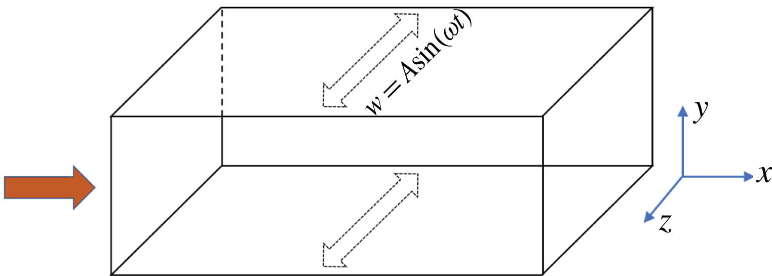
2.2 Flow configuration

Figure 1.

Schematic of the turbulent channel flow under SWO with amplitude $A$ and angular frequency $\unicode[STIX]{x1D714}$ ; $x$ , $y$ and $z$ denote the streamwise, wall-normal and spanwise directions, respectively.

Figure 1 shows a schematic of the turbulent channel flow, where $x$ and $z$ represent homogeneous streamwise and spanwise directions, respectively, in which periodic boundary conditions are imposed, and $y$ denotes the wall-normal direction. The isothermal wall boundary condition is employed, and the no-slip boundary conditions for velocities are applied, i.e. $(u_{i})_{w}=0$ . For the controlled cases, both walls move in unison with a periodic spanwise velocity, namely

(2.8) $$\begin{eqnarray}w_{w}(t)=A\sin (\unicode[STIX]{x1D714}t),\end{eqnarray}$$

where $A$ the velocity amplitude and $\unicode[STIX]{x1D714}=2\unicode[STIX]{x03C0}/T$ is the angular frequency.

Following Coleman et al. (Reference Coleman, Kim and Moser1995), the bulk Reynolds number is defined as $Re_{b}=\unicode[STIX]{x1D70C}_{b}U_{b}h/\unicode[STIX]{x1D707}_{w}$ , where $\unicode[STIX]{x1D707}_{w}$ is the dynamics viscosity on the wall, and bulk density $\unicode[STIX]{x1D70C}_{b}$ and bulk mean velocity $U_{b}$ are defined as

(2.9) $$\begin{eqnarray}\displaystyle \unicode[STIX]{x1D70C}_{b}=\frac{1}{2h}\int _{-h}^{h}\langle \unicode[STIX]{x1D70C}\rangle \,\text{d}y, & & \displaystyle\end{eqnarray}$$

(2.10) $$\begin{eqnarray}\displaystyle U_{b}=\frac{1}{2h\unicode[STIX]{x1D70C}_{b}}\int _{-h}^{h}\langle \unicode[STIX]{x1D70C}u\rangle \,\text{d}y, & & \displaystyle\end{eqnarray}$$

and the bulk Mach number is defined as

(2.11) $$\begin{eqnarray}M_{b}=U_{b}/c_{w},\end{eqnarray}$$

where $c_{w}$ is the speed of sound at the wall temperature. Following standard practice (Coleman et al. Reference Coleman, Kim and Moser1995), a spatially constant body force $f_{1}$ is applied in the streamwise direction in order to enforce constant mass flow rate in time, and the corresponding power spent is added to the right-hand side of the total energy equation.

2.3 Numerical set-up

A DNS of CTCF is performed with an in-house code. The governing equations are discretized based on the finite-difference method with a seventh-order upwind-biased scheme (Rai & Moin Reference Rai and Moin1991; Mittal & Moin Reference Mittal and Moin1997) for the convective terms and eighth-order centred scheme for the viscous terms. Time integration is done by using the low-storage third-order Runge–Kutta scheme. The mesh spacing is constant in the wall-parallel direction, and a mapping function is used in the wall-normal direction to cluster mesh points towards the wall. The DNS is carried out in a rectangular box whose sizes in the $x,y,z$ directions are denoted as $L_{x},L_{y},L_{z}$ . For the uncontrolled cases, all simulations are initiated with parabolic velocity profile plus superimposed random fluctuations and with uniform values for the temperature and density. For the controlled cases, all simulations start with the same initial condition of an uncontrolled fully developed turbulent channel flow at the same $Re_{b}$ and $M_{b}$ .

First, DNS is conducted at three different Mach numbers $M_{b}=0.3$ (nearly incompressible case), $0.8$ (subsonic case) and $1.5$ (supersonic case) with a fixed $Re_{b}=3000$ . The wall velocity amplitude was fixed at $A^{+}$ $(\equiv A/u_{\unicode[STIX]{x1D70F}})=12$ to enable comparison with previous incompressible results (Quadrio, Ricco & Viotti Reference Quadrio, Ricco and Viotti2009; Touber & Leschziner Reference Touber and Leschziner2012; Hurst et al. Reference Hurst, Yang and Chung2014). The oscillation period is varied as $T^{+}(\equiv Tu_{\unicode[STIX]{x1D70F}}^{2}/\unicode[STIX]{x1D708}_{w})\in [25,50,75,100,150,200,250,300]$ . 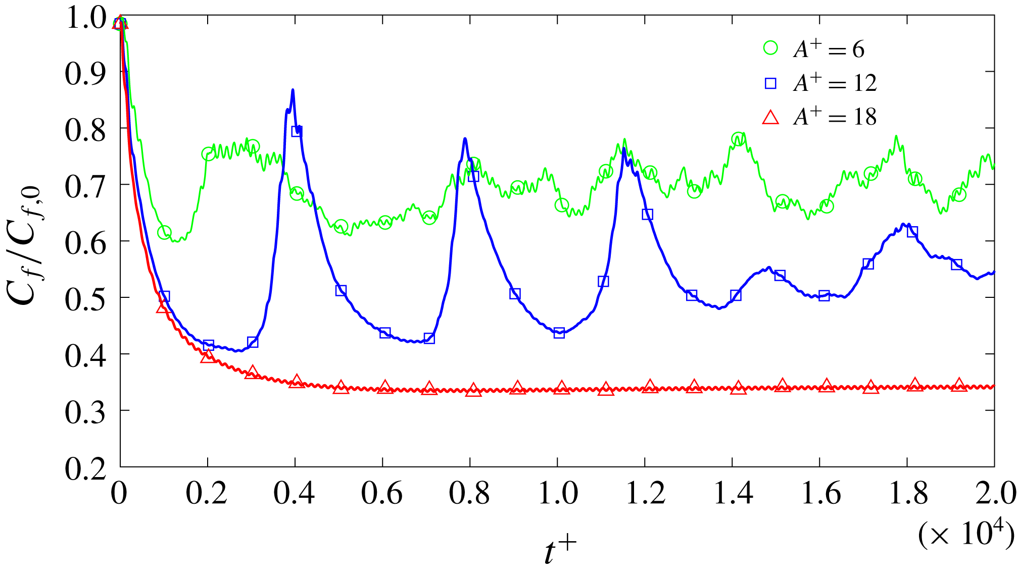(Throughout the paper, the control parameters are all non-dimensionalized by the wall units of the uncontrolled cases.) Then, two additional forcing amplitudes $A^{+}=6$ and $18$ are applied at $M_{b}=1.5$ to quantify the amplitude effect. 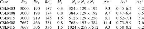Finally, to further investigate the Reynolds number effect, additional simulations are also performed at a higher $Re_{b}=7667$ for $M_{b}=0.8$ and $1.5$ cases. Details of the simulation parameters (i.e. grid sizes and resolutions) are given in table 1. All simulations are carried out with a constant time-marching step $\unicode[STIX]{x0394}t^{+}=0.025$ , with time averaging for statistics taken over at least $t^{+}(\equiv tu_{\unicode[STIX]{x1D70F}}^{2}/\unicode[STIX]{x1D708})=10\,000$ after the initial transition. The grid resolution employed here is nearly the same as that used by Modesti & Pirozzoli (Reference Modesti and Pirozzoli2016), who demonstrated the sufficiency of this resolution by a detailed sensitivity study. The computational box size is $6\unicode[STIX]{x03C0}h\times 2h\times 2\unicode[STIX]{x03C0}h$ ( $h$ is half of the channel height) for all cases. Note that, for incompressible flow, the adequacy of this box size has been well established for both the uncontrolled (Lozano-Duran & Jiménez Reference Lozano-Duran and Jiménez2014) and controlled (Gatti & Quadrio Reference Gatti and Quadrio2013; Hurst et al. Reference Hurst, Yang and Chung2014) cases. As the typical size of structures enlarges as $M_{b}$ increases, it might still be necessary to justify the adequacy of the current domain size for compressible cases. In the Appendix, we provide a detailed study and justification of the domain size on skin friction and drag reduction for the $Re_{b}=3000$ and $M_{b}=1.5$ case.

Table 1.

Details of the numerical discretization employed for the present simulations. The computational box size is $6\unicode[STIX]{x03C0}h\times 2h\times 2\unicode[STIX]{x03C0}h$ ( $h$ is the half-channel height) for all cases, and $N_{x}$ , $N_{y}$ and $N_{z}$ are the numbers of grid sizes in $x$ , $y$ and $z$ directions. Here $Re_{\unicode[STIX]{x1D70F}c}^{\ast }$ indicates the semi-local Reynolds number $Re_{\unicode[STIX]{x1D70F}}^{\ast }$ at the half-channel height.

For comparison, drag control for incompressible flows at two different friction Reynolds numbers $Re_{\unicode[STIX]{x1D70F}}$ is carried out. The numerical details are provided in table 2. The code used for the incompressible case is the same as the one used in our previous studies (Yao et al. Reference Yao, Chen and Hussain2019), built around the main solver developed by Lee & Moser (Reference Lee and Moser2015). The incompressible Navier–Stokes equations are solved using the method of Kim, Moin & Moser (Reference Kim, Moin and Moser1987), in which equations for the wall-normal vorticity and the Laplacian of the wall-normal velocity are time-advanced. This formulation has the advantage of satisfying the continuity constraint exactly while eliminating the pressure. A Fourier–Galerkin method is used in the streamwise and spanwise directions, while a seventh-order B-spline collocation method is used in the wall-normal direction. A low-storage implicit–explicit scheme based on third-order Runge–Kutta for the nonlinear terms and Crank–Nicolson for the viscous terms is used for time advance. The flow is driven by a pressure gradient, which is adjusted in time to ensure that the mass flux through the channel always remains constant. For more details about the code, the numerical methods and how the simulations are run, see Lee & Moser (Reference Lee and Moser2015).

Table 2.

Details of the numerical discretization employed for the incompressible turbulent channel simulations. The computational box size is $6\unicode[STIX]{x03C0}h\times 2h\times 2\unicode[STIX]{x03C0}h$ for all cases, and $N_{x}$ , $N_{y}$ and $N_{z}$ are the numbers of grid sizes.

2.4 Code validation

In the following, both Reynolds (ensemble) and Favre averaging (Huang et al. Reference Huang, Coleman and Bradshaw1995)

(2.12) $$\begin{eqnarray}\unicode[STIX]{x1D719}=\overline{\unicode[STIX]{x1D719}}+\unicode[STIX]{x1D719}^{\prime }=\widetilde{\unicode[STIX]{x1D719}}+\unicode[STIX]{x1D719}^{\prime \prime }\end{eqnarray}$$

are employed for flow statistics. In (2.12), $\overline{\unicode[STIX]{x1D719}}$ denotes Reynolds averaging (in the homogeneous space direction and in time) with fluctuation $\unicode[STIX]{x1D719}^{\prime }$ satisfying

(2.13) $$\begin{eqnarray}\overline{\unicode[STIX]{x1D719}^{\prime }}=0,\end{eqnarray}$$

and $\widetilde{\unicode[STIX]{x1D719}}$ denotes Favre averaging with fluctuation $\unicode[STIX]{x1D719}^{\prime \prime }$ defined as

(2.14) $$\begin{eqnarray}\displaystyle & \displaystyle \widetilde{\unicode[STIX]{x1D719}}=\overline{\unicode[STIX]{x1D70C}\unicode[STIX]{x1D719}}/\overline{\unicode[STIX]{x1D70C}}, & \displaystyle\end{eqnarray}$$

(2.15) $$\begin{eqnarray}\displaystyle & \displaystyle \unicode[STIX]{x1D719}^{\prime \prime }=\unicode[STIX]{x1D719}-\widetilde{\unicode[STIX]{x1D719}}. & \displaystyle\end{eqnarray}$$

Considering the periodic nature of the actuation, phase averaging is also employed and defined as

(2.16) $$\begin{eqnarray}\langle \unicode[STIX]{x1D719}\rangle (y,\unicode[STIX]{x1D711})=\frac{1}{N}\mathop{\sum }_{n=0}^{N-1}\frac{1}{L_{x}}\frac{1}{L_{z}}\int _{0}^{L_{x}}\int _{0}^{L_{z}}\unicode[STIX]{x1D719}(x,y,z,\unicode[STIX]{x1D711}+2\unicode[STIX]{x03C0}n)\,\text{d}x\,\text{d}z,\end{eqnarray}$$

where the averaging is applied at a fixed phase $\unicode[STIX]{x1D711}$ in the homogeneous directions, $\langle \cdot \rangle$ indicates a phase-averaged quantity and $N$ is the number of cycles during the integration time.

The Reynolds stress tensor is denoted as $\unicode[STIX]{x1D70F}_{ij}=\overline{\unicode[STIX]{x1D70C}}R_{ij}$ , with $R_{ij}=\widetilde{u_{i}^{\prime \prime }u_{j}^{\prime \prime }}=\widetilde{u_{i}u_{j}}-\widetilde{u_{i}}\widetilde{u_{j}}$ . Hereinafter, quantities made non-dimensional with respect to the wall friction velocity $u_{\unicode[STIX]{x1D70F}}=\sqrt{\unicode[STIX]{x1D70F}_{w}/\unicode[STIX]{x1D70C}_{w}}$ and the viscous length scale ( $\unicode[STIX]{x1D6FF}_{\unicode[STIX]{x1D708}}=\unicode[STIX]{x1D708}_{w}/u_{\unicode[STIX]{x1D70F}}$ , where $\unicode[STIX]{x1D708}=\unicode[STIX]{x1D707}/\unicode[STIX]{x1D70C}$ is the kinematic viscosity) are denoted with superscript $+$ . The friction Reynolds number is defined as the ratio of outer to viscous length scales, hence $Re_{\unicode[STIX]{x1D70F}}=h/\unicode[STIX]{x1D6FF}_{\unicode[STIX]{x1D708}}=u_{\unicode[STIX]{x1D70F}}h/\unicode[STIX]{x1D708}_{w}$ . Huang et al. (Reference Huang, Coleman and Bradshaw1995) suggested that normalizing the mean velocity and Reynolds stress profiles with respect to suitable semi-local wall units based on the local density and viscosity (i.e. $u_{\unicode[STIX]{x1D70F}}^{\ast }=\sqrt{\unicode[STIX]{x1D70F}_{w}/\overline{\unicode[STIX]{x1D70C}}}$ , $\unicode[STIX]{x1D6FF}_{\unicode[STIX]{x1D708}}^{\ast }=\overline{\unicode[STIX]{x1D708}}/u_{\unicode[STIX]{x1D70F}}^{\ast }$ ) yields better collapse of the flow statistics with incompressible flows. Accordingly, the semi-local Reynolds number is defined as $Re_{\unicode[STIX]{x1D70F}}^{\ast }=h/\unicode[STIX]{x1D6FF}_{\unicode[STIX]{x1D708}}^{\ast }=Re_{\unicode[STIX]{x1D70F}}\sqrt{(\overline{\unicode[STIX]{x1D70C}}/\overline{\unicode[STIX]{x1D70C}}_{w})}/(\overline{\unicode[STIX]{x1D707}}/\overline{\unicode[STIX]{x1D707}}_{w})$ . Note that for isothermal CTCF, $Re_{\unicode[STIX]{x1D70F}}^{\ast }=Re_{\unicode[STIX]{x1D70F}}$ at the wall and decreases towards the channel centre.

Figure 2.

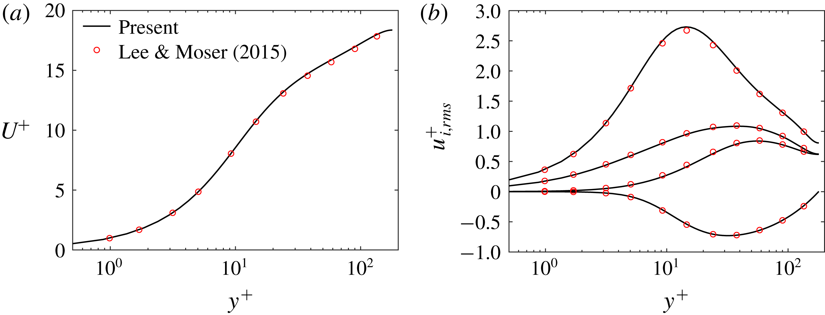
(a) Mean velocity ( $U^{+}(y^{+})$ ) and (b) root-mean-square of velocity fluctuations for the uncontrolled case at $Re_{b}=2880$ and $M_{b}=0.3$ . Solid lines represent our DNS results and circles are results from Lee & Moser (Reference Lee and Moser2015) at $Re_{\unicode[STIX]{x1D70F}}=180$ .

The compressible solver is first tested in the nearly incompressible case and compared with the strictly incompressible data of Lee & Moser (Reference Lee and Moser2015). Figure 2 shows the mean velocity profile $U^{+}$ and root-mean-square of velocity fluctuations, as well as the Reynolds shear stress ( $\overline{u^{\prime }v^{\prime }}$ ) for the uncontrolled case at $Re_{b}=2880$ and $M_{b}=0.3$ . 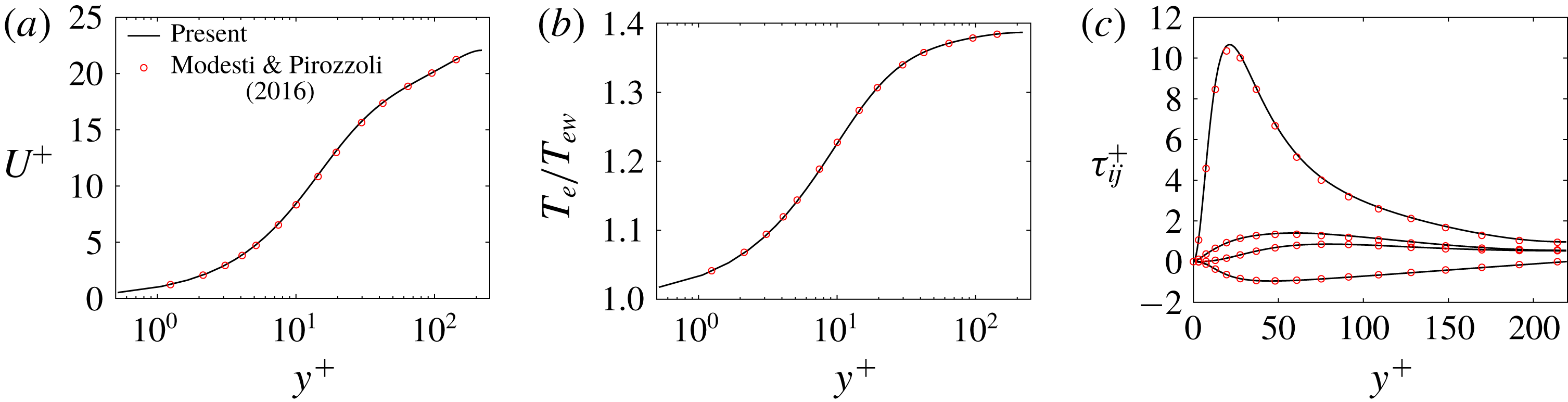Excellent agreement is observed in the mean-velocity profiles, the velocity fluctuations and Reynolds shear stress; except for the slight difference at the peak of the streamwise velocity fluctuations, which is known to be quite sensitive to discretization methods and mesh resolution (Bernardini, Pirozzoli & Orlandi Reference Bernardini, Pirozzoli and Orlandi2014). In addition to the incompressible case, the code is further validated with a supersonic case at $Re_{b}=3000$ and $M_{b}=1.5$ . Figure 3 shows a comparison of mean velocity $U^{+}$ , temperature $Te$ and Reynolds stresses $\unicode[STIX]{x1D70F}_{ij}$ between our results and those of Modesti & Pirozzoli (Reference Modesti and Pirozzoli2016). Our results show good congruence in all the flow statistics, suggesting the accuracy of our solver and adequacy of the grid resolution.

Figure 3.

Comparison with DNS data of Modesti & Pirozzoli (Reference Modesti and Pirozzoli2016) (circles) for $Re_{b}=3000$ and $M_{b}=1.5$ : (a) mean velocity ( $U^{+}(y^{+})$ ), (b) mean temperature ( $T_{e}/T_{ew}$ ) and (c) Reynolds normal and shear stresses ( $\unicode[STIX]{x1D70F}_{ij}$ ).

3.1 Drag reduction at $A^{+}=12$

Figure 4.

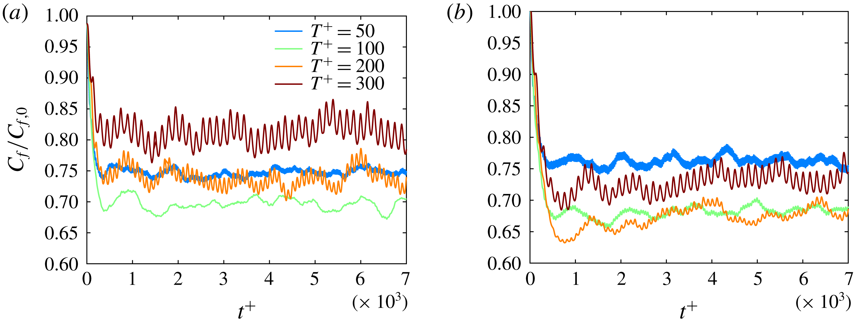
Initial time evolution ( $t^{+}\leqslant 7000$ ) of skin friction normalized by the uncontrolled case $C_{f}/C_{f,0}$ at different wall oscillation period $T^{+}$ with $A^{+}=12$ for $Re_{b}=3000$ and (a) $M_{b}=0.3$ , (b) $M_{b}=0.8$ and (c) $M_{b}=1.5$ .

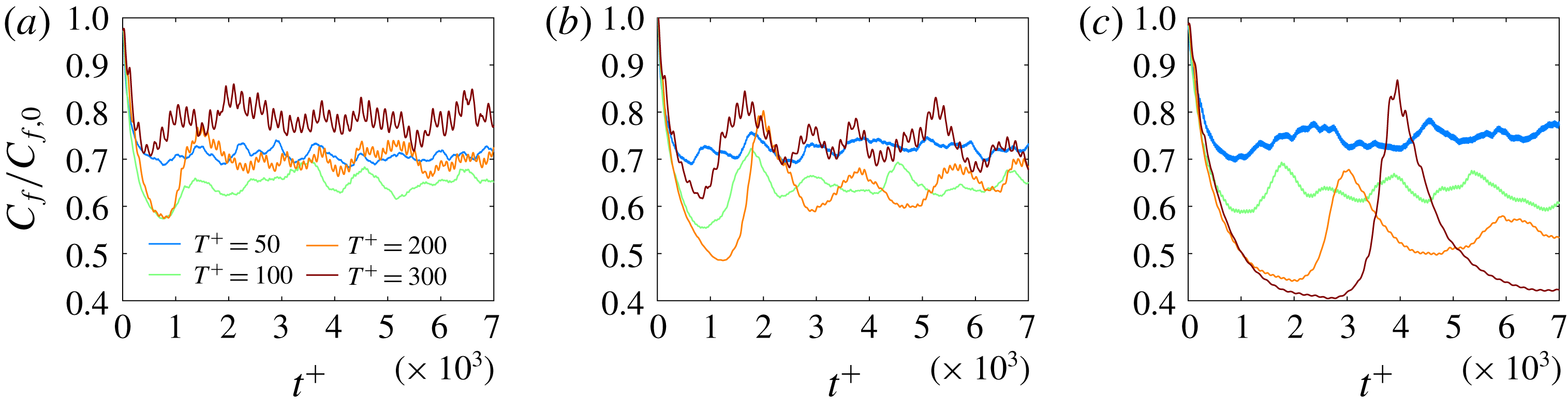
Figure 4 shows the early time evolution ( $t^{+}<7000$ ) of the skin friction coefficient $C_{f}(t)=2\unicode[STIX]{x1D70F}_{w}(t)/(\unicode[STIX]{x1D70C}_{b}U_{b}^{2})$ normalized by the uncontrolled value $C_{f,0}$ for different oscillation periods $T^{+}$ with $A^{+}=12$ at different $M_{b}$ values. Note that at a given time $t$ , $C_{f}(t)$ is obtained by averaging in the homogeneous directions. Some interesting features of figure 4 are summarized below.

(i) First, for the nearly incompressible cases (i.e. $M_{b}=0.3$ ), $C_{f}(t)$ initially rapidly decreases as the oscillation starts, and the decrease rates are very similar for all $T^{+}$ . Then, $C_{f}$ reaches a temporal minimum before approaching the statistical quasi-steady low-drag state. The long-time-scale undulation of $C_{f}$ , which has also been observed by others (Quadrio & Ricco Reference Quadrio and Ricco2003; Touber & Leschziner Reference Touber and Leschziner2012), is mainly because of the existence of large-scale turbulent structures – their augmentation/abatement leads to increase/decrease of $C_{f}$ . (Note that similar undulations also occur for flows in the absence of SWO.) First, the computational domain size, although considerably large when compared with the length scale of near-wall structures, accommodates only a few of these large-scale structures in both $x$ and $z$ directions. Therefore, averaging over the wall does not result in a converged constant value. Another issue is the periodic boundary condition imposed during the simulation. It has been shown that very large-scale structures, which can be significantly longer than typical streak length of $10^{3}$ wall units, can exist (Guala, Hommema & Adrian Reference Guala, Hommema and Adrian2006; Lozano-Durán & Jiménez Reference Lozano-Durán and Jiménez2014). Since the streamwise domain of our simulation is around $4\times 10^{3}$ wall units, these structures are not fully decorrelated because of $x$ -periodicity of the domain, and hence recycled.

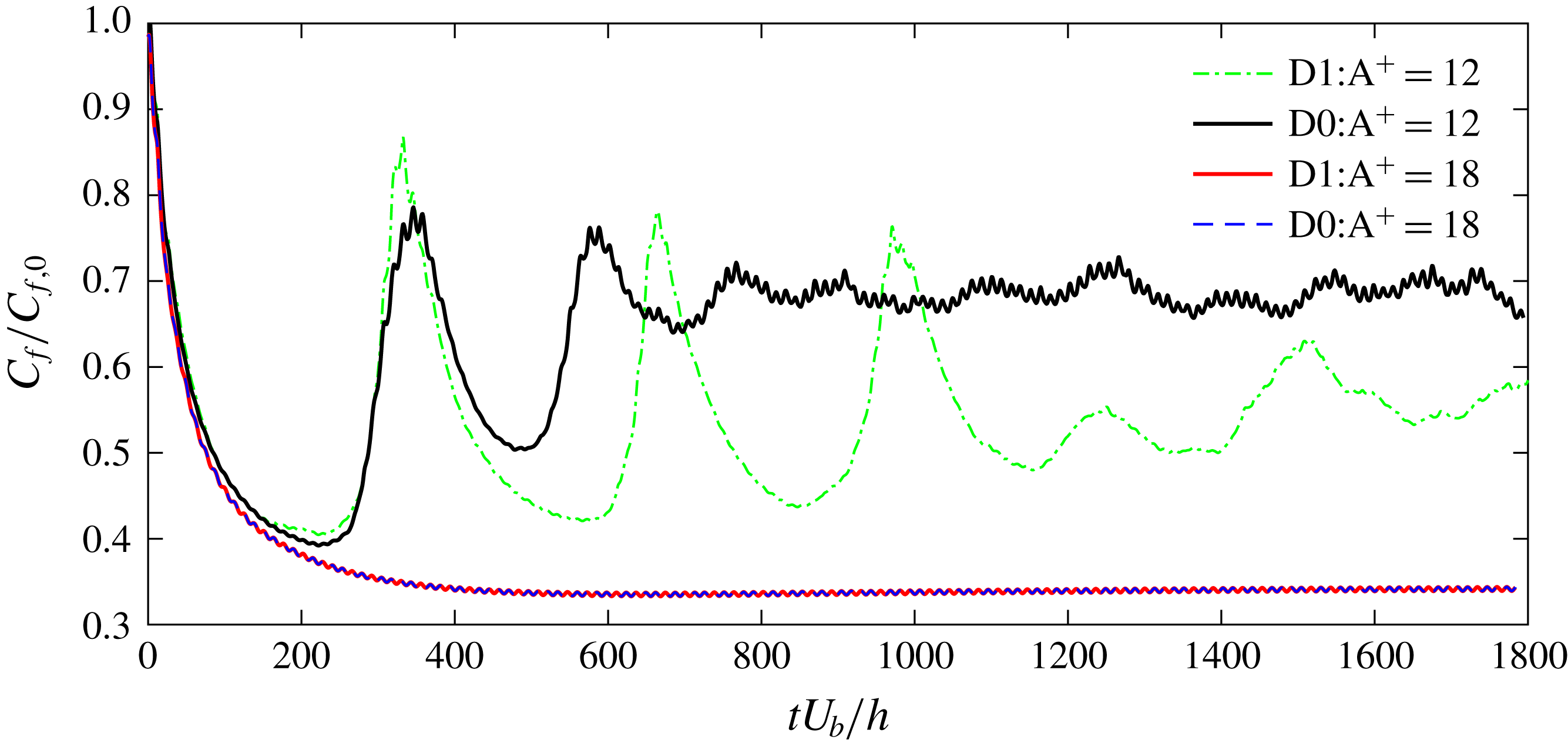
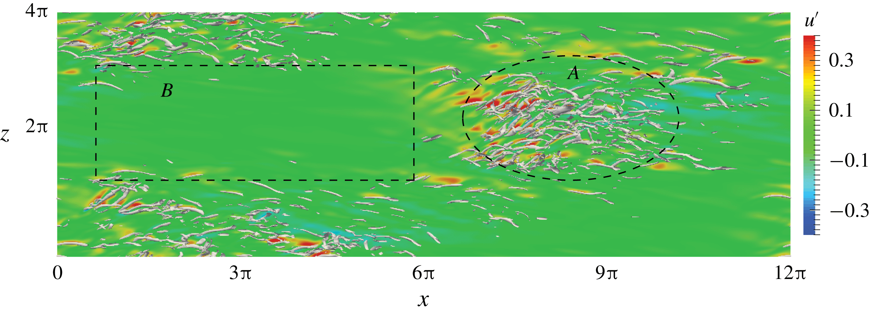
(ii) For the compressible cases, the long-time-scale undulation of $C_{f}$ becomes more apparent, especially for high drag reduction cases. One reason is that, as $M_{b}$ increases, the length scale of the large-scale structures increases; hence the computational domain includes even fewer of these structures (e.g. see figure 14). In addition, due to the relatively small Reynolds number involved ( $Re_{\unicode[STIX]{x1D70F}c}^{\ast }<200$ ), the drag-reducing flow is barely turbulent and becomes transitional. One example is the case of $T^{+}=300$ at $M_{b}=1.5$ (figure 4 c), where $C_{f}$ experiences continued rapid increases and decreases. Flow is almost relaminarized at $t^{+}\approx 2600$ ; the flow then regenerates the vortical structures to reach another peak at $t^{+}=4100$ ; and this quasi-cyclical process continues for many periods (see figure 16 for a longer time evolution). These in combination explain the larger temporal fluctuation of spatially averaged skin friction $C_{f}(t)$ observed for $M_{b}=0.8$ and $1.5$ cases.

Figure 5.

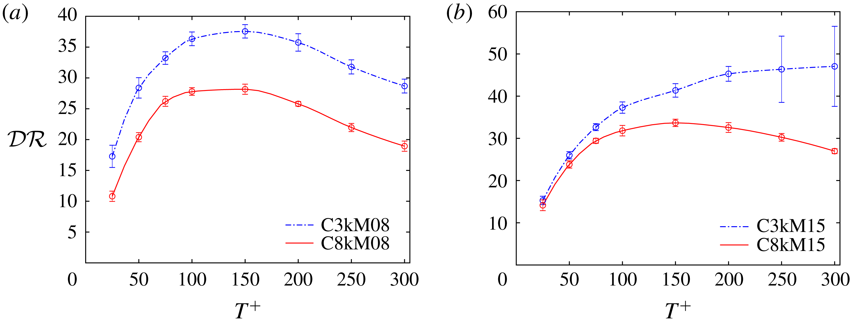
Drag reduction rate ${\mathcal{D}}{\mathcal{R}}$ (%) as a function of $T^{+}$ at $Re_{b}=3000$ for (a) different $M_{b}$ at $A^{+}=12$ and (b) different $A^{+}$ at $M_{b}=1.5$ . The error bars indicate the corresponding uncertainty of ${\mathcal{D}}{\mathcal{R}}$ .

(iii) For the nearly incompressible cases (i.e. $M_{b}=0.3$ ), $C_{f}$ hardly responds to the actuation at small $T^{+}$ (i.e. $T^{+}=50$ ); while substantial small-scale $C_{f}$ undulations, with half the wall oscillation period, occur for large $T^{+}$ , which is due to the turbulence responding to the wall actuation – the near-wall structures have enough time to develop their inner dynamics between successive activation of the near-wall Stokes layer (Quadrio & Ricco Reference Quadrio and Ricco2004; Touber & Leschziner Reference Touber and Leschziner2012). However, as $M_{b}$ increases, undulation in $C_{f}$ at small $T^{+}$ increases (note that the thicker curve for $T^{+}=50$ in figure 4(c) is due to very high-frequency oscillations, not visible in this compressed time curve). This high-frequency behaviour is further compounded by the fact that dispassion at this high frequency is significantly enhanced as the thermodynamic properties are altered (discussed in detail later).

We define the extent of drag reduction as

(3.1) $$\begin{eqnarray}{\mathcal{D}}{\mathcal{R}}\,(\%)=1-\overline{C}_{f}/\overline{C}_{f,0}.\end{eqnarray}$$

And its uncertainty is calculated by following the procedure in Gatti & Quadrio (Reference Gatti and Quadrio2016). First, the standard uncertainty $\unicode[STIX]{x1D70E}_{\overline{C}_{f}}$ of $\overline{C}_{f}$ is calculated via an autoregressive method as described by Oliver et al. (Reference Oliver, Malaya, Ulerich and Moser2014). Then the standard uncertainty $\unicode[STIX]{x1D70E}_{{\mathcal{D}}{\mathcal{R}}}$ of ${\mathcal{D}}{\mathcal{R}}$ is obtained by propagating the standard uncertainty of $\overline{C}_{f}$ for the uncontrolled and controlled cases (assuming they are independent variables (Gatti & Quadrio Reference Gatti and Quadrio2013)), i.e. $\unicode[STIX]{x1D70E}_{{\mathcal{D}}{\mathcal{R}}}=(\overline{C}_{f}/\overline{C}_{f,0})\sqrt{(\unicode[STIX]{x1D70E}_{\overline{C}_{f}}/\overline{C}_{f})^{2}+(\unicode[STIX]{x1D70E}_{\overline{C}_{f,0}}/\overline{C}_{f,0})^{2}}$ . Finally, the uncertainty is extended to a $95\,\%$ confidence interval $\unicode[STIX]{x1D6FF}_{{\mathcal{D}}{\mathcal{R}}}=z\unicode[STIX]{x1D70E}_{{\mathcal{D}}{\mathcal{R}}}$ , where $z=1.96$ is the standardized $95\,\%$ confidence interval of a normalized Gaussian probability density function. The uncertainty of ${\mathcal{D}}{\mathcal{R}}$ is reported in the text when applicable and plotted as error bars in the figures. Note that since the control parameters considered are mainly located in the region of negative net power saving, the energy cost and total net power saving rate are not addressed here.

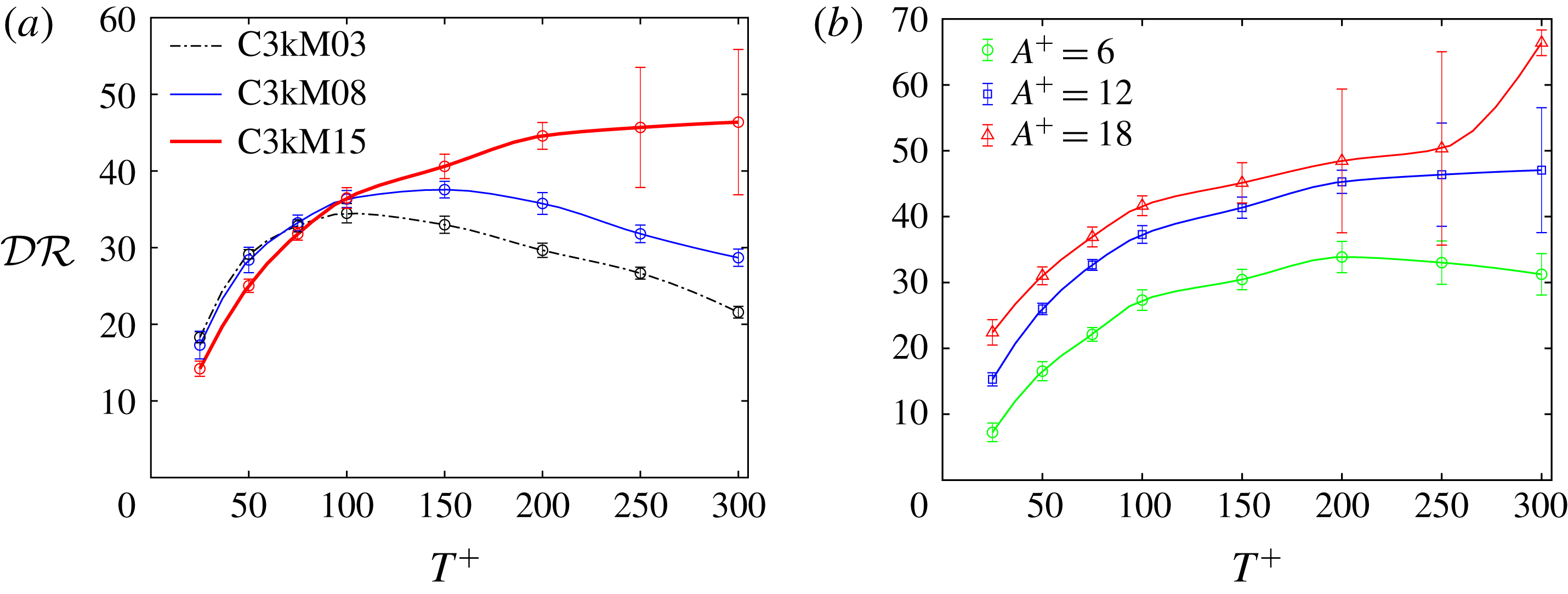
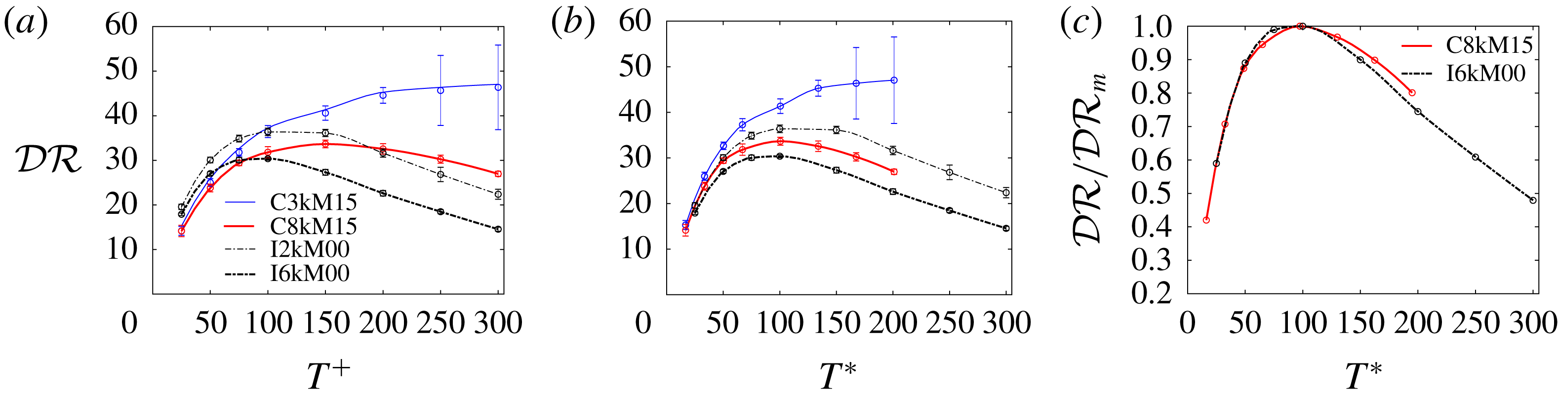
Figure 5(a) shows ${\mathcal{D}}{\mathcal{R}}$ against the oscillation period $T^{+}$ with an amplitude of $A^{+}=12$ for all $M_{b}$ cases at $Re_{b}=3000$ . First, for the nearly incompressible $M_{b}=0.3$ case, the present results agree with those of Touber & Leschziner (Reference Touber and Leschziner2012), Gatti & Quadrio (Reference Gatti and Quadrio2013), Hurst et al. (Reference Hurst, Yang and Chung2014) and Yao et al. (Reference Yao, Chen and Hussain2019) at $Re_{\unicode[STIX]{x1D70F}}=200$ . The maximum drag reduction ${\mathcal{D}}{\mathcal{R}}_{max}=34.8\,\%\pm 0.9\,\%$ with the optimal oscillation period $T_{opt}^{+}=100$ ; both of these agree well with the results of Yao et al. (Reference Yao, Chen and Hussain2019). Note that our results are also close to the $36.4\,\%$ of Hurst et al. (Reference Hurst, Yang and Chung2014) and $37.4\,\%$ of Gatti & Quadrio (Reference Gatti and Quadrio2016) (the latter is slightly higher due to smaller domain size used, which causes overestimation of ${\mathcal{D}}{\mathcal{R}}$ in the region close to the optimal period, as reported by Gatti & Quadrio (Reference Gatti and Quadrio2013)). For $M_{b}=0.8$ , ${\mathcal{D}}{\mathcal{R}}$ exhibits a similar trend to the $M_{b}=0.3$ case, namely ${\mathcal{D}}{\mathcal{R}}$ increases with $T^{+}$ to a maximum and then decreases gradually. However, compared with the $M_{b}=0.3$ case, ${\mathcal{D}}{\mathcal{R}}$ at $M_{b}=0.8$ slightly decreases at small $T^{+}$ (i.e. ${\leqslant}100$ ), but increases at large $T^{+}$ . The optimal oscillation period is shifted to $T_{opt}^{+}=150$ , with ${\mathcal{D}}{\mathcal{R}}_{max}=37.6\,\%\pm 1.1\,\%$ – slightly higher than that obtained at $M_{b}=0.3$ . At $M_{b}=1.5$ , ${\mathcal{D}}{\mathcal{R}}$ further decreases at small $T^{+}$ but, interestingly, increases monotonically with $T^{+}$ . At $T^{+}=300$ , the largest oscillation period considered, ${\mathcal{D}}{\mathcal{R}}$ reaches $47.1\,\%\pm 8.1\,\%$ . The large uncertainty is attributed to the low Reynolds number effect, where the flow continues to undulate in time between laminar and turbulent states.

3.2 Mean density and temperature profiles

Figure 6.

Mean density $\overline{\unicode[STIX]{x1D70C}}$ and temperature $\overline{T}_{e}$ profiles for different oscillating period $T^{+}$ with $A^{+}=12$ for (a) $M_{b}=0.8$ and (b) $M_{b}=1.5$ with $Re_{b}=3000$ . (c) The temperature at the channel centre $\overline{T}_{ec}$ and density at the wall $\overline{\unicode[STIX]{x1D70C}}_{w}$ as a function of $T^{+}$ for both cases.

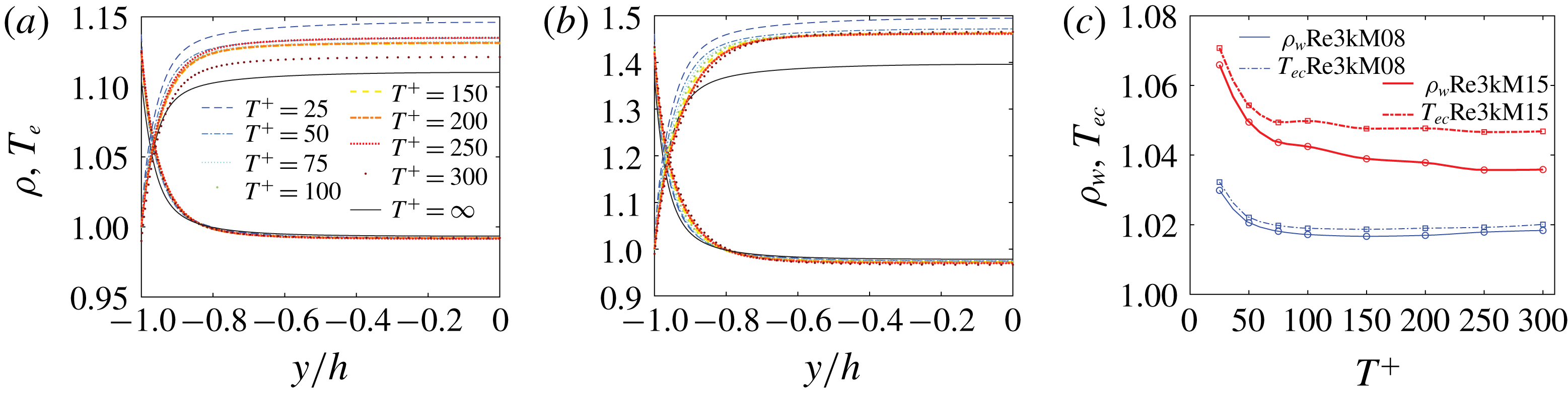
Profiles of the Reynolds-averaged density $\overline{\unicode[STIX]{x1D70C}}$ and temperature $\overline{T}_{e}$ for different oscillation periods $T^{+}$ are displayed in figures 6(a) and 6(b) for $M_{b}=0.8$ and $1.5$ , respectively. The results for the $M_{b}=0.3$ case are not shown since the temperature and density are barely changed. For both $M_{b}=0.8$ and $1.5$ cases, $\overline{T}_{e}$ rises steeply near the wall and reaches a plateau in the core region; correspondingly, $\overline{\unicode[STIX]{x1D70C}}$ decreases rapidly near the wall and then reaches a plateau in the channel core (Foysi et al. Reference Foysi, Sarkar and Friedrich2004). The temperature at the centre of the channel $\overline{T}_{ec}$ and density at the wall $\overline{\unicode[STIX]{x1D70C}}_{w}$ increase with $M_{b}$ , which is due to enhanced viscous heating. Under SWO, as a consequence of the dissipation of the Stokes layer, a significant increase of the mean temperature first occurs near the wall and then diffuses over the whole channel, particularly for cases with smaller $T^{+}$ (or larger $\unicode[STIX]{x1D714}^{+}$ ), as expected. It is different with the turbulent boundary layer case (Ni et al. Reference Ni, Lu, Ribault and Fang2016), where the effect of the Stokes layer on the mean temperature profiles is mainly limited to the near-wall region, as the time needed for diffusion along the wall direction, before the flow is advected downstream, is not available. Accordingly, under SWO, the mean density $\overline{\unicode[STIX]{x1D70C}}$ at the wall also increases, while $\overline{\unicode[STIX]{x1D70C}}$ is only slightly affected in the core region, where the compressible effect is rather weak. The temperature at the centre $\overline{T}_{ec}$ and the density on the wall $\overline{\unicode[STIX]{x1D70C}}_{w}$ as a function of $T^{+}$ are further displayed in figure 6(c). Both $\overline{T}_{ec}$ and $\overline{\unicode[STIX]{x1D70C}}_{w}$ increase as $T^{+}$ decreases (or $\unicode[STIX]{x1D714}^{+}$ increases), with a rapid increase of $\overline{T}_{ec}$ and $\unicode[STIX]{x1D70C}_{w}$ for very small $T^{+}$ . The variation of these thermodynamic properties will be found to play a role in affecting the drag control performance; this role is different from the control with uniform blowing and suction (Kametani et al. Reference Kametani, Kotake, Fukagata and Tokugawa2017), where $\overline{\unicode[STIX]{x1D70C}}_{w}$ and $\overline{T}_{ec}$ are not significantly altered.

3.3 Mean spanwise velocity profiles

Figure 7.

Phase-averaged spanwise velocity profiles $\langle w\rangle ^{+}$ for $T^{+}=100$ and $A^{+}=12$ as a function of (a) wall-normal coordinate $y^{+}$ and as function of oscillation phase $\unicode[STIX]{x1D711}$ at (b) $\unicode[STIX]{x1D702}=1$ ( $y^{+}\approx 6$ ) and (c) $\unicode[STIX]{x1D702}=\unicode[STIX]{x03C0}$ ( $y^{+}\approx 19$ ). Note that the incompressible laminar Stokes layer solutions are also included for comparison, with the vertical dashed line in (a) denoting the Stokes layer thickness.

In the case of wall-oscillation-induced fluid only, the flow develops the Stokes layer, whose profiles, in the incompressible limit, are given by (Batchelor Reference Batchelor1967)

(3.2) $$\begin{eqnarray}W(y,t)=A\text{e}^{-\unicode[STIX]{x1D702}}\sin (\unicode[STIX]{x1D714}t-\unicode[STIX]{x1D702}),\end{eqnarray}$$

where $\unicode[STIX]{x1D702}=y\sqrt{\unicode[STIX]{x1D714}/2\unicode[STIX]{x1D708}}$ .

Previous incompressible studies have shown that the Stokes layer induced in turbulent channel flow agrees with the laminar analytical solution for relatively small oscillation period $T^{+}$ , where the Stokes layer is within the viscous sublayer (Quadrio & Sibilla Reference Quadrio and Sibilla2000; Touber & Leschziner Reference Touber and Leschziner2012). For the compressible case, the Stokes layer also depends on the fluid properties, like density and viscosity, whose values change along the wall-normal direction and change with the phase of oscillation, as well as the control parameters, i.e. wall oscillation amplitude $A^{+}$ and frequency $\unicode[STIX]{x1D714}^{+}$ . 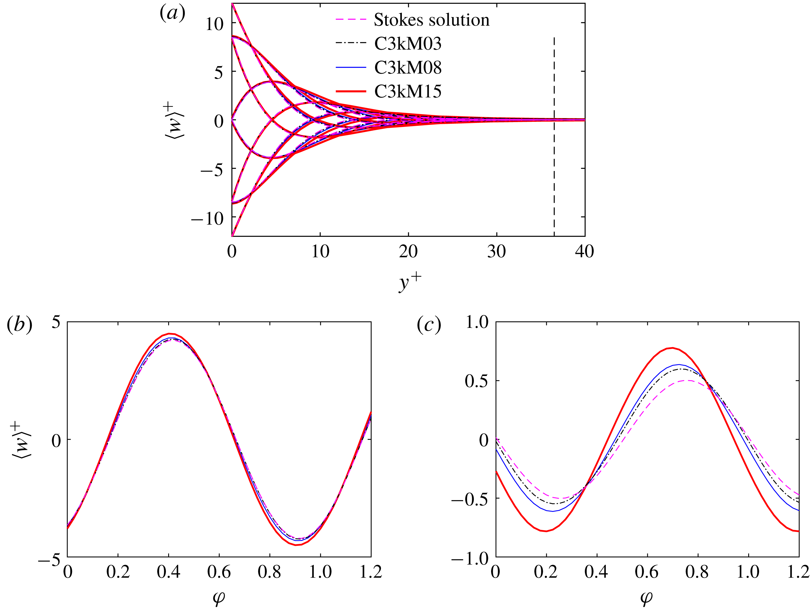Hence, equation (3.2), in general, is no longer valid. However, it might still be interesting to compare the phase-averaged spanwise velocity with the incompressible laminar Stokes layer profiles. Figure 7(a) shows the phase-averaged spanwise velocity $\langle w\rangle ^{+}$ profiles for $T^{+}=100$ for all $M_{b}$ cases, along with the incompressible laminar Stokes flow solution (3.2). The laminar Stokes layer thickness is $\unicode[STIX]{x1D6FF}^{+}=\sqrt{4\unicode[STIX]{x03C0}T^{+}}$ in wall units, which is $\unicode[STIX]{x1D6FF}^{+}=35.4$ for $T^{+}=100$ . A detailed comparison of the spanwise velocity profiles as a function of the oscillation phase $\unicode[STIX]{x1D711}$ at different wall-normal locations $y^{+}$ is presented in figure 7(b,c). Interestingly, very close to the wall, e.g. at $\unicode[STIX]{x1D702}=1$ (corresponding to $y^{+}=6$ ), $\langle w\rangle ^{+}$ is quite similar to the Stokes layer profiles even for the $M_{b}=1.5$ case. However, further away from the wall, $\langle w\rangle ^{+}$ deviates from the incompressible laminar Stokes profile, even for the $M_{b}=0.3$ case. In particular, the phase difference between DNS and incompressible laminar Stokes profile increases with $M_{b}$ , and the amplitude of $\langle w\rangle ^{+}$ decays slower for larger $M_{b}$ cases. Note that with increasing $M_{b}$ , the fluid viscosity near the wall increases; hence the phase variation along the wall-normal direction decreases below that in the incompressible case – progressively more at even higher $M_{b}$ .

3.4 Mean streamwise velocity profiles

Figure 8.

Mean velocity profiles transformed according to (a) van Driest (Reference van Driest1951) and (b) Trettel & Larsson (Reference Trettel and Larsson2016) for $Re_{b}=3000$ at all $M_{b}$ values. The dashed lines represent the law of the wall: linear law $U^{+}=y^{+}$ and log law $U^{+}=(1/\unicode[STIX]{x1D705})\ln y^{+}+B$ with $\unicode[STIX]{x1D705}=0.41$ and $B=5.2$ .

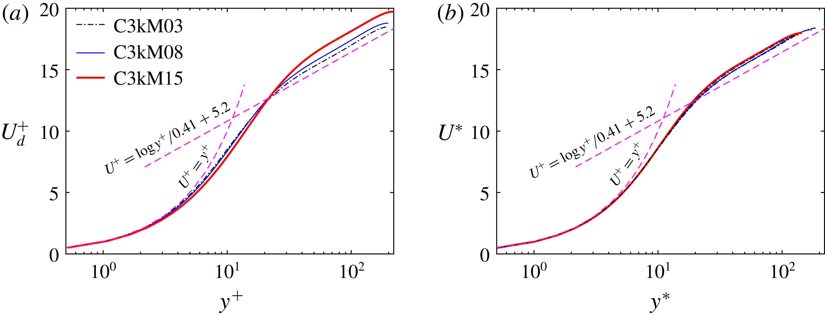
It is known that classical wall unit scaling fails in collapsing the velocity profiles when the compressibility effect is present. To incorporate the effect of density variation, the van Driest transformation (van Driest Reference van Driest1951), defined as

(3.3) $$\begin{eqnarray}U_{d}^{+}=\int _{0}^{U^{+}}\sqrt{\frac{\overline{\unicode[STIX]{x1D70C}}}{\overline{\unicode[STIX]{x1D70C}}_{w}}}\,\text{d}U^{+},\end{eqnarray}$$

has typically been employed to collapse velocity profiles of supersonic flows with those of incompressible flows. The success of the density-weighted scaling can be attributed to Morkovin’s hypothesis, which assumes that, for moderate Mach numbers, the compressibility effect on turbulence could be accounted for by the mean density variations alone. The van Driest transformation has been shown to be good in collapsing velocity profiles of supersonic flows over adiabatic walls (Duan, Beekman & Martin Reference Duan, Beekman and Martin2010; Pirozzoli & Bernardini Reference Pirozzoli and Bernardini2011; Hadjadj et al. Reference Hadjadj, Ben-Nasr, Shadloo and Chaudhuri2015). However, the van Driest transformation fails to capture the correct intercept of the log law for diabatic walls, and the deviation increases for cases with strong heat flux (Duan et al. Reference Duan, Beekman and Martin2010). Figure 8(a) shows the mean velocity profiles based on the van Driest transformation as a function of $y^{+}$ for the uncontrolled cases for all three $M_{b}$ cases. Also included in the figure are the law of the wall: $U^{+}=y^{+}$ and $U^{+}=(1/\unicode[STIX]{x1D705})\ln y^{+}+B$ , where $\unicode[STIX]{x1D705}=0.41$ and $B=5.2$ . The van Driest transformation yields the correct log-layer profile. Consistent with the previous results (Modesti & Pirozzoli Reference Modesti and Pirozzoli2016; Patel et al. Reference Patel, Boersma and Pecnik2016), the van Driest transformation visibly undershoots the incompressible velocity profile in the viscous sublayer and overshoots in the log layer, especially for the $M_{b}=1.5$ case.

Trettel & Larsson (Reference Trettel and Larsson2016) derived a transformation that could incorporate the wall-normal density and viscosity gradients:

(3.4) $$\begin{eqnarray}\displaystyle U^{\ast }=\int _{0}^{U^{+}}\sqrt{\frac{\overline{\unicode[STIX]{x1D70C}}}{\overline{\unicode[STIX]{x1D70C}}_{w}}}\left[1+\frac{1}{2\overline{\unicode[STIX]{x1D70C}}}\frac{\text{d}\overline{\unicode[STIX]{x1D70C}}}{\text{d}y}y-\frac{1}{\overline{\unicode[STIX]{x1D707}}}\frac{\text{d}\overline{\unicode[STIX]{x1D707}}}{\text{d}y}y\right]\text{d}U^{+}, & & \displaystyle\end{eqnarray}$$

which has been shown to successfully collapse mean velocity profiles for supersonic channel flows with isothermally cooled walls (Modesti & Pirozzoli Reference Modesti and Pirozzoli2016; Zhang, Duan & Choudhari Reference Zhang, Duan and Choudhari2018). By rescaling the Navier–Stokes equations using the local mean properties and semi-local friction velocity, Patel et al. (Reference Patel, Boersma and Pecnik2016) derived an equivalent mean velocity transform as

(3.5) $$\begin{eqnarray}U^{\ast }=\int _{0}^{U_{d}}\left(1+\frac{y}{Re_{\unicode[STIX]{x1D70F}}^{\ast }}\frac{\text{d}Re_{\unicode[STIX]{x1D70F}}^{\ast }}{\text{d}y}\right)\text{d}U_{d}.\end{eqnarray}$$

Figure 8(b) further shows the mean velocity profiles according to the transformation of Trettel & Larsson (Reference Trettel and Larsson2016) for all three $M_{b}$ cases. Note that the wall-normal distance is non-dimensionalized using the semi-local scaling $y^{\ast }$ $(=yRe_{\unicode[STIX]{x1D70F}}^{\ast })$ . Apparently, the limitation of the van Driest transformation is overcome by this transformation, which yields overall good collapse among all the profiles across the whole wall-normal range.

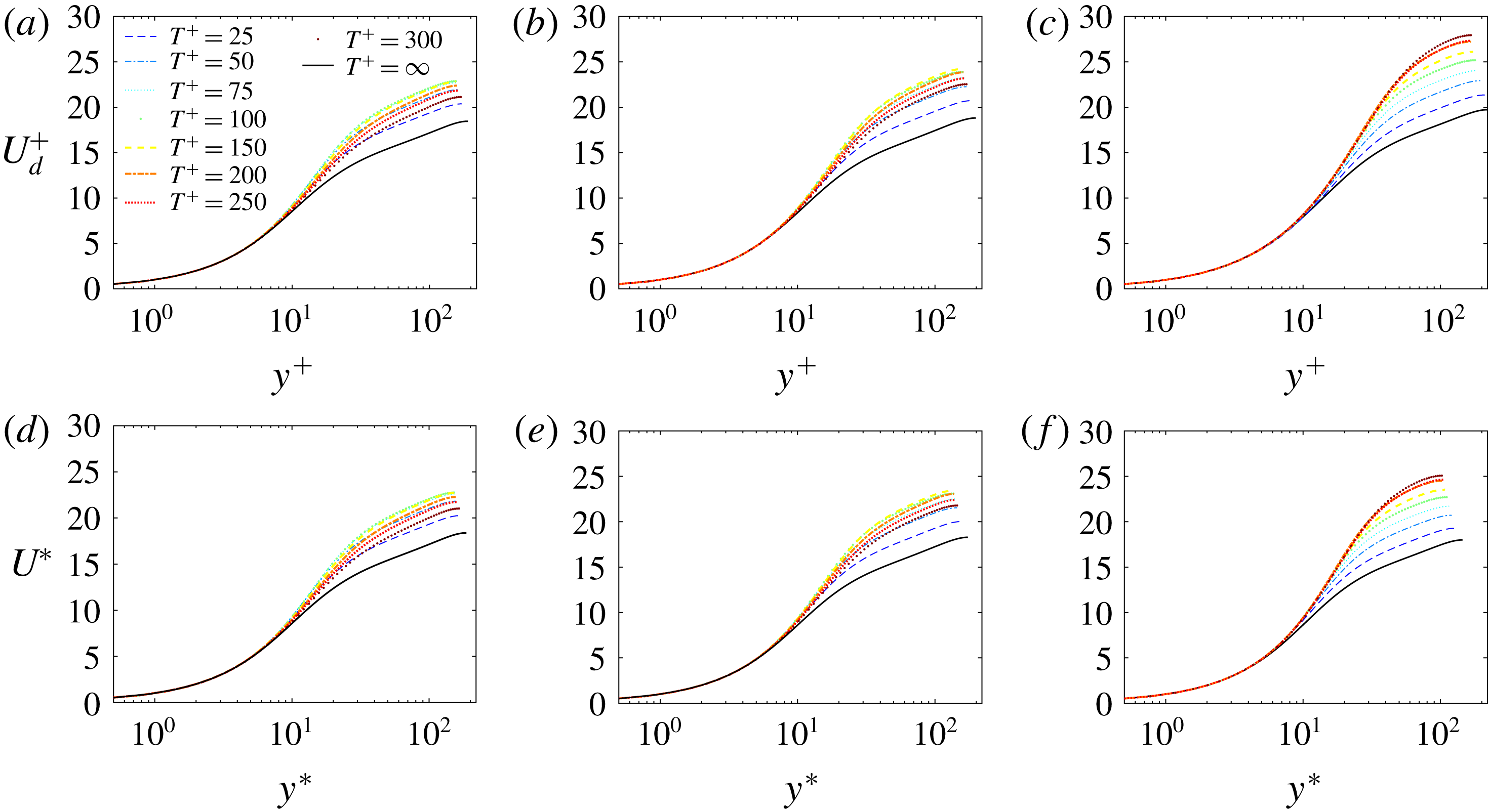
The mean velocity profiles based on both van Driest and Trettel–Larsson transformations under SWO with different $T^{+}$ at $A^{+}=12$ for all $M_{b}$ cases are displayed in figure 9. Consistent with the incompressible control cases (Touber & Leschziner Reference Touber and Leschziner2012; Hurst et al. Reference Hurst, Yang and Chung2014), under control the velocity profiles in the log-law region show a characteristic upward shift when the $u_{\unicode[STIX]{x1D70F}}$ value for each controlled flow is used for scaling; the magnitude of the upward shift is roughly proportional to ${\mathcal{D}}{\mathcal{R}}$ . This is rather interesting but not surprising, because with increasing ${\mathcal{D}}{\mathcal{R}}$ the viscous layer becomes thicker, and the log layer is, therefore, shifted upward (not unlike similar shift by roughness on the wall). At this low $Re_{b}$ , the mean velocity profiles slowly transform towards laminar profiles for high ${\mathcal{D}}{\mathcal{R}}$ cases; hence the log law becomes less distinct, which is more evident at large $T^{+}$ for the $M_{b}=1.5$ case (figure 9 f).

Figure 9.

Transformed mean streamwise velocity profiles for different oscillation periods $T^{+}$ with $A^{+}=12$ for (a,d) $M_{b}=0.3$ , (b,e) $M_{b}=0.8$ and (c,f) $M_{b}=1.5$ . (a–c) The van Driest transformation and (d–f) the Trettel–Larsson transformation. Note that $T^{+}=\infty$ (the lowest curve) denotes the uncontrolled case.

3.5 Reynolds stress and FIK identity

Figure 10.

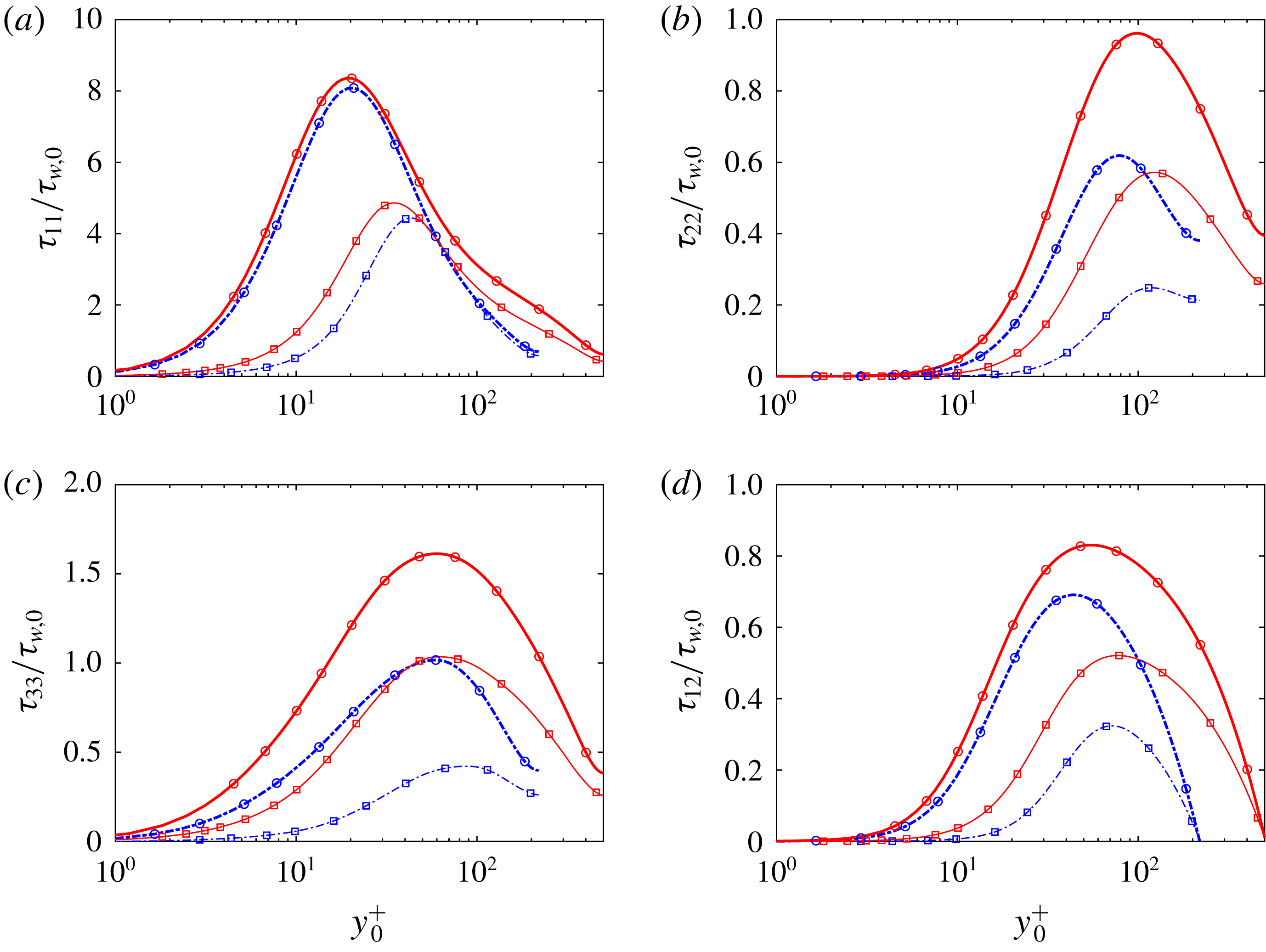
Reynolds normal stress components (normalized by the wall shear stress of the uncontrolled case $\unicode[STIX]{x1D70F}_{w,0}$ ) as a function of $y_{0}^{+}$ for different oscillation periods $T^{+}$ at $A^{+}=12$ for (a,d,g) $M_{b}=0.3$ , (b,e,h) $M_{b}=0.8$ and (c,f,i) $M_{b}=1.5$ . Rows (a–c), (d–f) and (g–i) correspond to $\unicode[STIX]{x1D70F}_{11}$ , $\unicode[STIX]{x1D70F}_{22}$ and $\unicode[STIX]{x1D70F}_{33}$ , respectively.

The effect of control on turbulent fluctuations is further scrutinized. Figure 10 shows the Reynolds normal stresses ( $\unicode[STIX]{x1D70F}_{11}$ , $\unicode[STIX]{x1D70F}_{22}$ and $\unicode[STIX]{x1D70F}_{33}$ ) as a function of $y_{0}^{+}$ with different oscillation period $T^{+}$ at $A^{+}=12$ . To highlight the absolute changes under control, the Reynolds stresses are normalized with the wall shear stress $\unicode[STIX]{x1D70F}_{w,0}$ for the uncontrolled cases. Note that scaling with the controlled wall shear stress would be indicative of universal viscous scaling, which we do not focus on here.

Let us first focus on the streamwise Reynolds stress $\unicode[STIX]{x1D70F}_{11}$ . For the uncontrolled case, the peak value increases as $M_{b}$ increases; and the peak location also slightly moves outward, namely changing from $y^{+}\approx 15$ at $M_{b}=0.3$ to $y^{+}\approx 20$ at $M_{b}=1.5$ . Note that when semi-local coordinates $y^{\ast }$ are used, a better match among different $M_{b}$ cases, especially for the peak location, can be obtained – to be discussed later. Under control, the stress is overall suppressed in the whole range of wall-normal coordinate, especially for the large ${\mathcal{D}}{\mathcal{R}}$ cases. Compared to the uncontrolled case, the peak location moves away from the wall under control, which is consistent with the observation in the strictly incompressible cases (Hurst et al. Reference Hurst, Yang and Chung2014; Yao et al. Reference Yao, Chen and Hussain2019) as well as for other control methods (Choi et al. Reference Choi, Moin and Kim1994; Deng et al. Reference Deng, Xu, Huang and Cui2014). The peak value and the peak location also seem to change systematically with ${\mathcal{D}}{\mathcal{R}}$ : namely, strong suppression of the peak value and large outward shift of peak location occur for large ${\mathcal{D}}{\mathcal{R}}$ .

In contrast to the increase of the peak of $\unicode[STIX]{x1D70F}_{11}$ , the peak of wall-normal Reynolds stress $\unicode[STIX]{x1D70F}_{22}$ for the uncontrolled case decreases with increasing $M_{b}$ . Similar is the case for both spanwise Reynolds stress $\unicode[STIX]{x1D70F}_{33}$ and Reynolds shear stress $\unicode[STIX]{x1D70F}_{12}$ . We give a qualitative explanation of the difference of increasing $M_{b}$ on $\unicode[STIX]{x1D70F}_{11}$ and $\unicode[STIX]{x1D70F}_{22}$ . The reason is that, as $M_{b}$ increases, temperature increases, and so does the viscosity – suppressing the ejection and sweep events of near-wall streamwise vortices, thus leading to lower values of the peak in $\unicode[STIX]{x1D70F}_{22}$ (Sciacovelli, Cinnella & Gloerfelt Reference Sciacovelli, Cinnella and Gloerfelt2017). This is different from $\unicode[STIX]{x1D70F}_{11}$ , where the peak is increased due to mean shear ( $\text{d}U/\text{d}y$ ), which is higher in the case of high $M_{b}$ . The effect of control on wall-normal stress is similar to that on streamwise Reynolds stress.

However, the behaviour of spanwise Reynolds stress $\unicode[STIX]{x1D70F}_{33}$ under control is different: it develops a near-wall peak at large $T^{+}$ for $M_{b}=0.3$ , which even exceeds the uncontrolled cases indicating the reduced effectiveness of control at large $T^{+}$ . A similar effect was explained by Touber & Leschziner (Reference Touber and Leschziner2012) via both statistical and structural approaches. Statistically, a production term associated with the shear strain of the Stokes layer significantly contributes to the budget of $\unicode[STIX]{x1D70F}_{33}$ and enhances it. The production term is typically much lower at smaller $T^{+}$ , due to the fact that the level of turbulence is highly suppressed, but is significantly increased at large $T^{+}$ . Structurally, SWO introduces a periodic realignment of the streak, whose tilting angle depends on the ratio between spanwise and streamwise velocity strain $(\text{d}\langle w\rangle /\text{d}y)/(\text{d}\langle u\rangle /\text{d}y)$ , and the angle generally increases with $T^{+}$ due to increased spanwise strain. This realignment gives rise to a spanwise component of the velocity fluctuation in the inclined streak direction, and thus to an enhancement of $\unicode[STIX]{x1D70F}_{33}$ . The near-wall peak decreases with increasing $M_{b}$ and becomes less obvious for the $M_{b}=1.5$ case. This is because the streamwise velocity strain ( $\text{d}\langle u\rangle /\text{d}y$ ) is much stronger at high $M_{b}$ . Hence, the tilting angle and reorientation are also suppressed at high $M_{b}$ for large $T^{+}$ – resulting in higher ${\mathcal{D}}{\mathcal{R}}$ .

Figure 11.

Reynolds shear stresses $\unicode[STIX]{x1D70F}_{12}$ normalized by the wall shear stress of the uncontrolled case $\unicode[STIX]{x1D70F}_{w,0}$ for different oscillation periods $T^{+}$ at $A^{+}=12$ for (a) $M_{b}=0.3$ , (b) $M_{b}=0.8$ and (c) $M_{b}=1.5$ .

Since the Reynolds shear stress $\unicode[STIX]{x1D70F}_{12}$ is strongly linked to the skin-friction drag (Fukagata et al. Reference Fukagata, Iwamoto and Kasagi2002), figure 11 further examines $\unicode[STIX]{x1D70F}_{12}$ profiles (normalized by the wall shear stress of the uncontrolled case $\unicode[STIX]{x1D70F}_{w,0}$ ) in outer scaling. Similar to other Reynolds stress components, $\unicode[STIX]{x1D70F}_{12}$ is substantially decreased under control, especially close to the wall, consistent with the fact that the peak also moves away from the wall. The decrease in the maximum value correlates with ${\mathcal{D}}{\mathcal{R}}$ . For example, the peak of $\unicode[STIX]{x1D70F}_{12}$ at $T^{+}=300$ for $M_{b}=1.5$ drops about 60 %, in absolute value, consistent with the decrease in total skin friction of around 45 % when contributions from other parts are included, like the laminar part, discussed later.

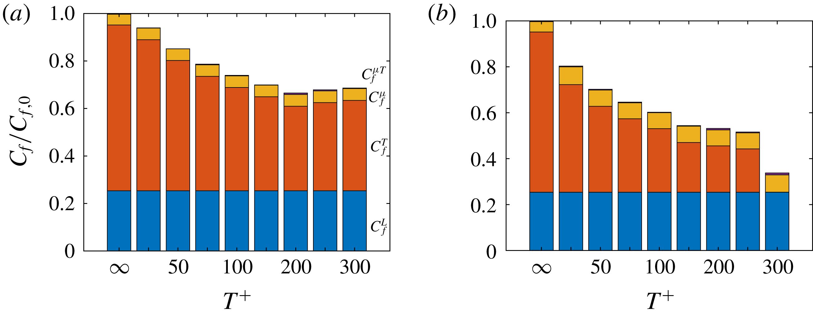
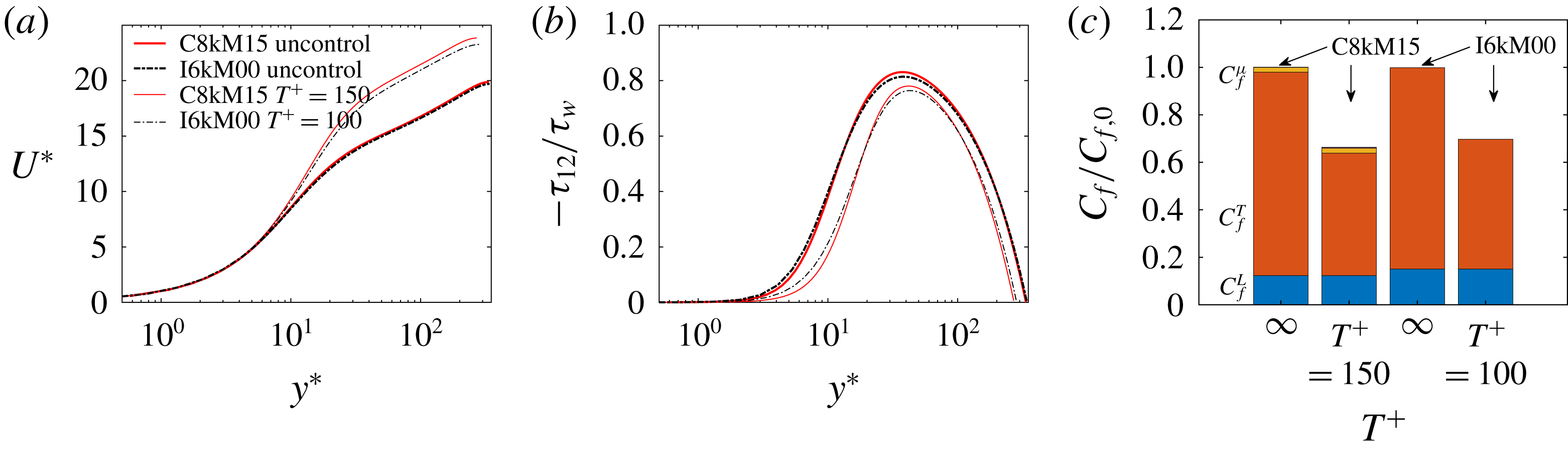
Based on the compressible flow version of the FIK identity derived by Gomez et al. (Reference Gomez, Flutet and Sagaut2009), the physical decomposition of the total skin friction can be expressed as

(3.6) $$\begin{eqnarray}\displaystyle C_{f} & = & \displaystyle \underbrace{\frac{6}{Re_{b}}}_{C_{f}^{L}}+\underbrace{3\int _{-1}^{1}y\overline{\unicode[STIX]{x1D70C}}\widetilde{u^{\prime \prime }v^{\prime \prime }}\,\text{d}y}_{C_{f}^{T}}\nonumber\\ \displaystyle & & \displaystyle +\,\underbrace{\frac{3}{Re_{b}}\int _{-1}^{1}y\left(\frac{\overline{\unicode[STIX]{x1D707}}}{\overline{\unicode[STIX]{x1D707}}_{w}}-1\right)\frac{\unicode[STIX]{x2202}\overline{u}}{\unicode[STIX]{x2202}y}\text{d}y}_{C_{f}^{\unicode[STIX]{x1D707}}}+\underbrace{\frac{3}{Re_{b}}\int _{-1}^{1}y\overline{\unicode[STIX]{x1D707}^{\prime }\left(\frac{\unicode[STIX]{x2202}u^{\prime }}{\unicode[STIX]{x2202}y}+\frac{\unicode[STIX]{x2202}v^{\prime }}{\unicode[STIX]{x2202}x}\right)}\,\text{d}y}_{C_{f}^{\unicode[STIX]{x1D707}T}},\end{eqnarray}$$

which decomposes the skin friction into four components: an ‘equivalent’ laminar part $C_{f}^{L}$ ; a turbulent part $C_{f}^{T}$ represented by the weighted integration of the total Reynolds shear stress; the compressible contribution $C_{f}^{\unicode[STIX]{x1D707}}$ related to the mean viscosity variations and the mean wall-normal velocity gradient; and the compressible–turbulent interaction part $C_{f}^{\unicode[STIX]{x1D707}T}$ . Note that the latter two terms, absent for the strictly incompressible case, together contribute less than $0.3\,\%$ of the total skin friction for our nearly incompressible case (i.e. $M_{b}=0.3$ ), hence are ignored in the following discussion. The weight in the integration decreases linearly with increasing distance from the wall, which clearly highlights the contribution of near-wall turbulent structures to the skin friction.

The decomposed total skin friction $C_{f}$ (normalized by the uncontrolled case $C_{f,0}$ ) for different oscillation periods $T^{+}$ is depicted in figure 12 for different $M_{b}$ cases. First, the compressible–turbulent interaction term $C_{f}^{\unicode[STIX]{x1D707}T}$ is negligible (less than $0.4\,\%$ for all cases). This is also confirmed by Zhe et al. (Reference Zhe, ChangPing, Li and XinLiang2016) even for an $M=6$ hypersonic turbulent boundary layer. Since $Re_{b}$ is fixed, $C_{f}^{L}$ is held constant for all cases, which contributes approximately $25\,\%$ of the total $C_{f}$ for the uncontrolled case. The compressible contribution term $C_{f}^{\unicode[STIX]{x1D707}}$ is also small, and increases as $M_{b}$ increases, becoming $1.3\,\%$ at $M_{b}=0.8$ and $4.5\,\%$ at $M_{b}=1.5$ . Hence, $C_{f}^{T}$ is the dominant contribution for the total $C_{f}$ (similar to the incompressible case), and its contribution gradually decreases as $M_{b}$ increases, being $75.0\,\%$ , $73.5\,\%$ and $69.8\,\%$ at $M_{b}=0.3$ , $0.8$ and $1.5$ , respectively.

Figure 12.

Decomposed skin friction $C_{f}$ (normalized by the uncontrolled case $C_{f,0}$ ) for different oscillation periods $T^{+}$ at $A^{+}=12$ for (a) $M_{b}=0.3$ , (b) $M_{b}=0.8$ and (c) $M_{b}=1.5$ . Note that $T^{+}=\infty$ denotes the uncontrolled case.

Parenthetically, since the normalized skin friction $C_{f}/C_{f,0}$ is $1-{\mathcal{D}}{\mathcal{R}}$ , its variation with respect to $T^{+}$ is just opposite to that for ${\mathcal{D}}{\mathcal{R}}$ (figure 5 a). Under control, $C_{f}^{\unicode[STIX]{x1D707}}$ is only slightly altered for the $M_{b}=0.8$ case. For example, $C_{f}^{\unicode[STIX]{x1D707}}/C_{f,0}$ increases to approximately $1.8\,\%$ for $T^{+}=25$ , the smallest oscillation period considered. The slight alteration is understandable since the temperature (hence also viscosity) is only mildly altered by SWO for the subsonic cases. Besides, the integrand of $C_{f}^{\unicode[STIX]{x1D707}}$ is very small near the wall as $\overline{\unicode[STIX]{x1D707}}/\overline{\unicode[STIX]{x1D707}}_{w}-1$ goes to zero near the wall. For the $M_{b}=1.5$ case, the contribution of $C_{f}^{\unicode[STIX]{x1D707}}$ further increases, due to increased viscosity under SWO. In particular, the contribution of $C_{f}^{\unicode[STIX]{x1D707}}$ increases to approximately $6.0\,\%$ of the total $C_{f,0}$ at $T^{+}=25$ , which partially explains why ${\mathcal{D}}{\mathcal{R}}$ deteriorates at small $T^{+}$ . For $M_{b}=0.3$ , the reduction in total $C_{f}$ is only due to the decrease in $C_{f}^{T}$ (corresponding to the suppression of the turbulent Reynolds shear stress). From figure 12, it is obvious that, even for the $M_{b}=1.5$ case, the reduction in total $C_{f}$ is also mainly due to the decrease in $C_{f}^{T}$ .

3.6 Energy spectrum

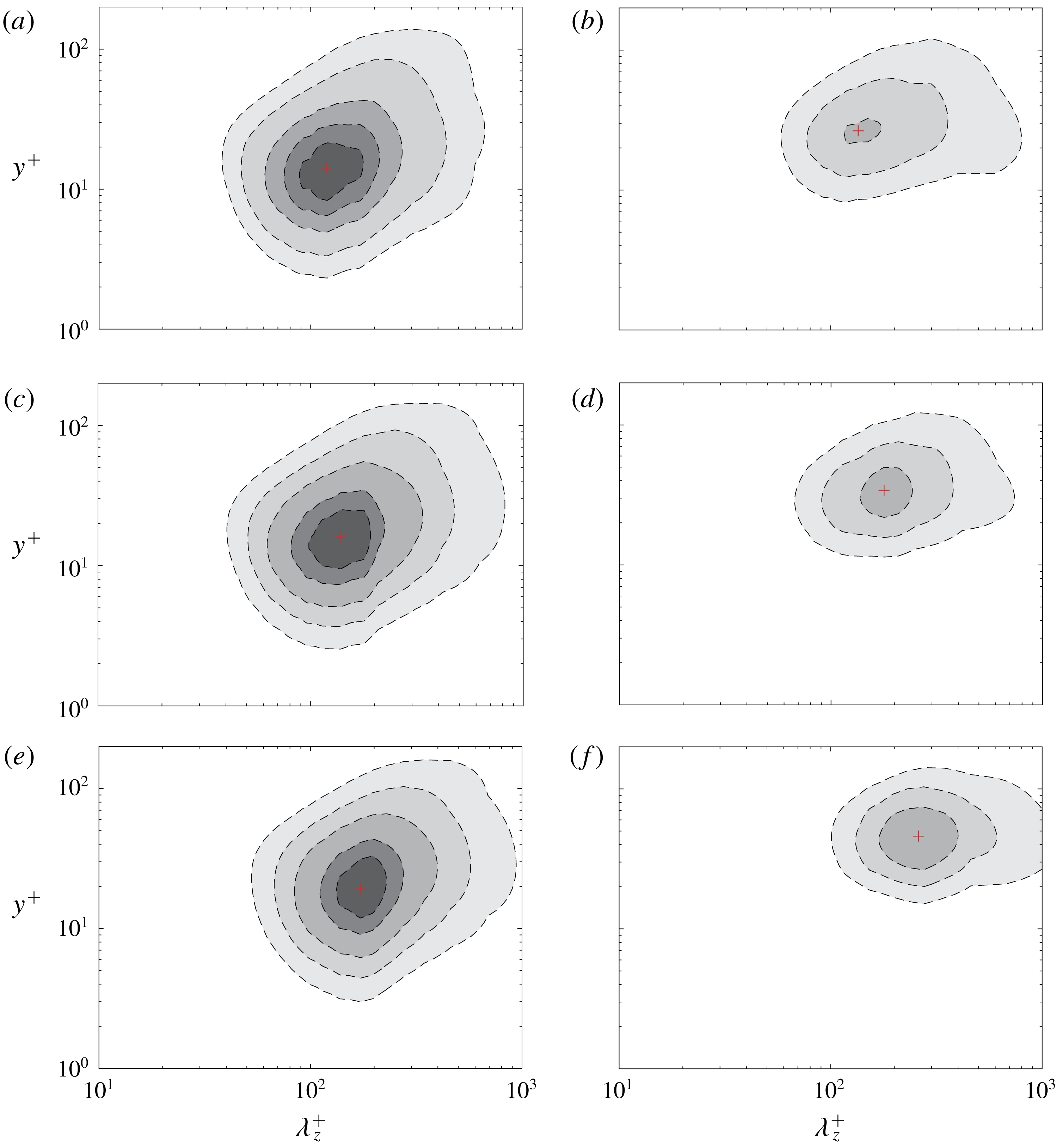
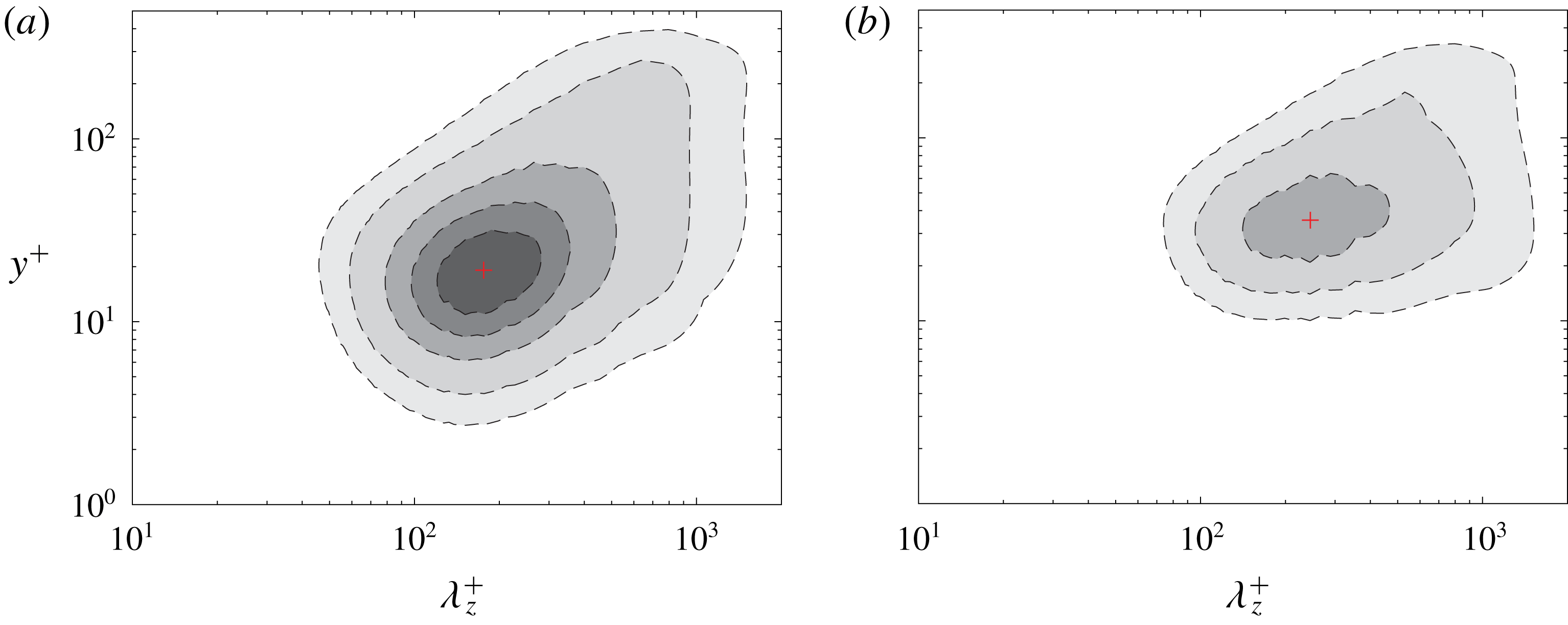
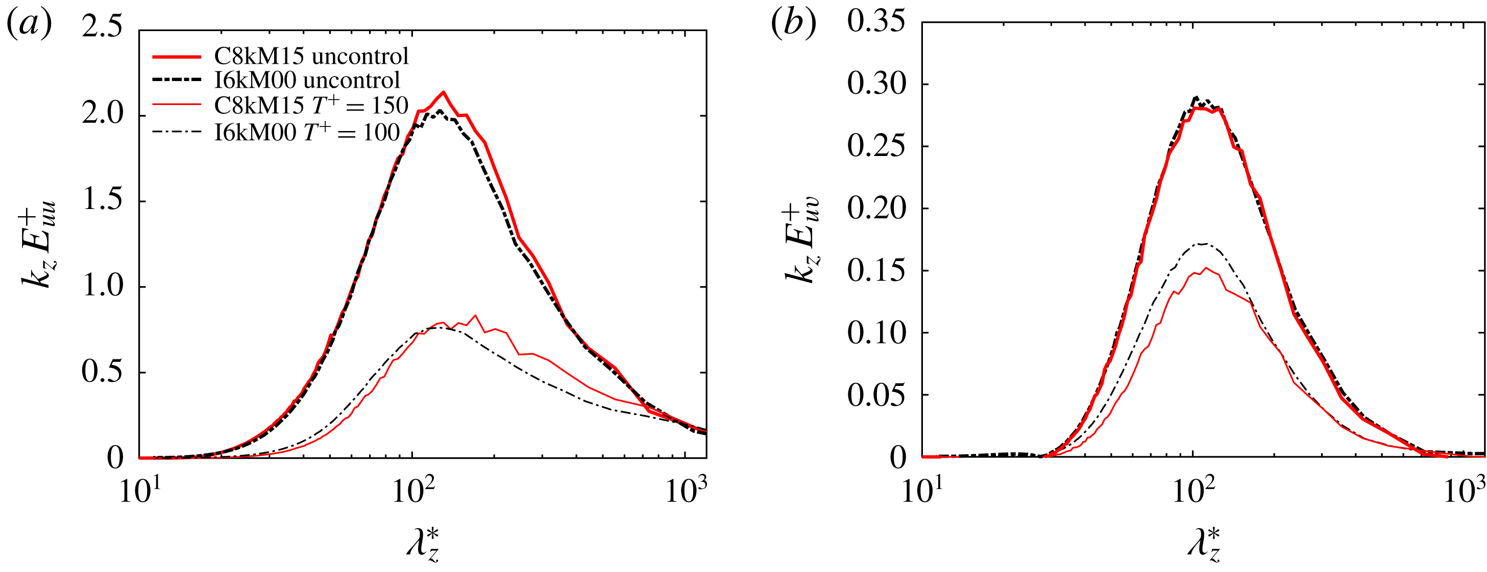
Figure 13 compares the pre-multiplied spanwise spectrum of streamwise velocity $k_{z}E_{uu}$ (normalized by the maximum value of the uncontrolled case) as a function of spanwise wavelength $\unicode[STIX]{x1D706}_{z}^{+}$ between the uncontrolled and controlled cases. Here, the near-optimal control period with $T^{+}=150$ is considered. The peak location of the spectrum, denoted as $+$ in the figure, typically represents the mean streak spacing. 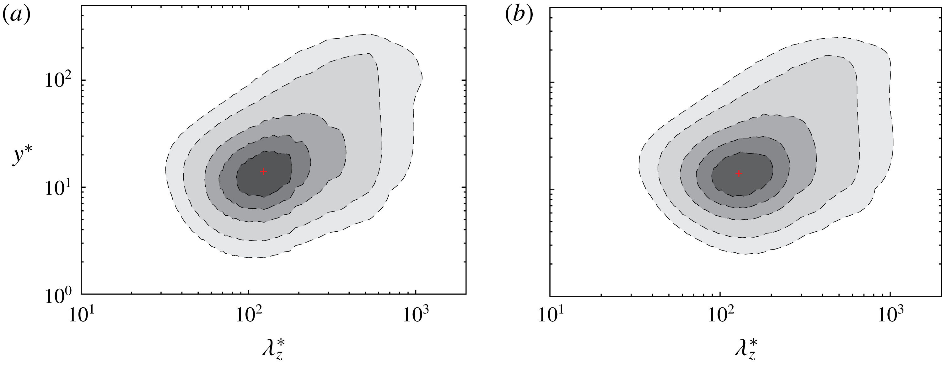For incompressible flows, the near-wall streak spacing in the viscous sublayer is typically of the order of $10^{2}$ wall units and remains remarkably constant over a wide range of Reynolds numbers (Lozano-Durán & Jiménez Reference Lozano-Durán and Jiménez2014). Figure 13 shows that the streak spacing increases with $M_{b}$ when scaled in wall units. In particular, the wavelength increases from $\unicode[STIX]{x1D706}_{z}^{+}\approx 120$ for $M_{b}=0.3$ to $\unicode[STIX]{x1D706}_{z}^{+}\approx 140$ for $M_{b}=0.8$ and to $\unicode[STIX]{x1D706}_{z}^{+}\approx 175$ for $M_{b}=1.5$ . Also, the wall-normal location of the peak also increases as $M_{b}$ increases, which is consistent with an outward shift of the streamwise Reynolds stress in figure 10. Compared with the uncontrolled case, the contribution from the near-wall region is effectively suppressed, especially at higher $M_{b}$ , and the energy-containing part is also shifted outward with a much weaker peak. This suggests that the streaks under SWO are significantly weakened, which is further confirmed with the flow visualization shown below.

Figure 13.

Pre-multiplied spanwise spectrum of streamwise velocity $k_{z}E_{uu}$ (normalized by the maximum value of uncontrolled case) as a function of $\unicode[STIX]{x1D706}_{z}^{+}$ at $Re_{b}=3000$ for (a,b) $M_{b}=0.3$ , (c,d) $M_{b}=0.8$ and (e,f) $M_{b}=1.5$ . (a,c,e) Uncontrolled and (b,d,f) controlled cases with $A^{+}=12$ and $T^{+}=150$ . The $+$ symbol denotes the location of maximum value.

3.7 Coherent structures

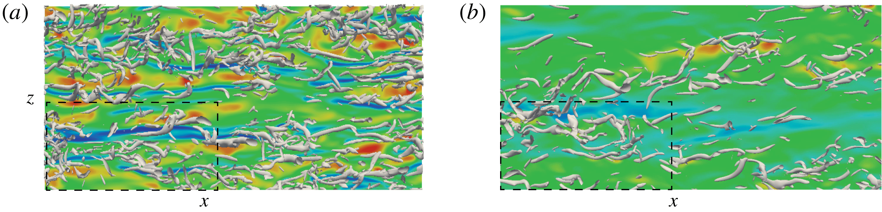
The effect of control on near-wall coherent structures is examined. Figure 14 shows the top view of instantaneous vortical structures visualized using $\unicode[STIX]{x1D706}_{\unicode[STIX]{x1D70C}}$ criterion (Yao & Hussain Reference Yao and Hussain2018) for both uncontrolled and controlled (for $T^{+}=150$ ) cases; also shown are the streaks at $y^{+}\approx 15$ . Note that the time selected for the controlled cases is around the same oscillation phase for all $M_{b}$ cases. For the uncontrolled case at $M_{b}=0.3$ , typical meandering low-speed streak structures are observed aligned along the streamwise directions; and the streamwise vortices are mainly located near the interface of low- and high-speed streaks. As $M_{b}$ increases, the streaks become more coherent (longer and less wavy), and hence more stable (Patel et al. Reference Patel, Boersma and Pecnik2016). Correspondingly, the streamwise vortices are more sparsely distributed and elongated. Similar observations have been reported by Coleman et al. (Reference Coleman, Kim and Moser1995) for supersonic turbulent channel flow and by Duan et al. (Reference Duan, Beekman and Martin2010) for supersonic turbulent boundary layers with cooled walls. Patel et al. (Reference Patel, Boersma and Pecnik2016) showed that, for the $dRe_{\unicode[STIX]{x1D70F}}^{\ast }/dy<0$ case (typical of all flows considered in this paper), the inclining and tilting of the vortices decrease, and the streaks are more stabilized compared with the constant-property case.

Figure 14.

Top view of instantaneous vortical structures (visualized using $\unicode[STIX]{x1D706}_{\unicode[STIX]{x1D70C}}^{+}$ ) associated with the streamwise velocity fluctuations (streaks) $|u^{\prime }/U_{b}|<0.4$ at $y^{+}\approx 15$ for $Re_{b}=3000$ and $M_{b}=$ (a,b) $0.3$ , (c,d) $0.8$ and (e,f) $1.5$ . (a,c,e) Uncontrolled and (b,d,f) controlled cases with $T^{+}=150$ . The red (dark) and blue (light) correspond to positive and negative fluctuations. Note that the domain size is $L_{x}\times L_{z}=6\unicode[STIX]{x03C0}h\times 2\unicode[STIX]{x03C0}h$ .

Compared with the uncontrolled cases, the strength of the streaks is significantly weakened under control. Consequently, the generation of drag-inducing near-wall streamwise vortices is also suppressed, especially for the $M_{b}=1.5$ case, where only a few vortices are observed. Besides, the streaks are tilted along the spanwise direction. This is similar to that reported in Touber & Leschziner (Reference Touber and Leschziner2012), where the near-wall streaks are periodically reoriented based on the phase of the oscillation – a consequence of the competing effect of the streamwise and spanwise velocity components. While the bulk flow tries to align the low-speed streaks in the streamwise direction, simultaneously a spanwise velocity component due to SWO tends to tilt the streak to the spanwise direction. Touber & Leschziner (Reference Touber and Leschziner2012) showed that the spanwise tilting angle of the streaks coincides with the angle of the mean shear $(\text{d}\langle w\rangle /\text{d}y)/(\text{d}\langle u\rangle /\text{d}y)$ around $y^{+}=10$ . Using conditional averaging, Yakeno et al. (Reference Yakeno, Hasegawa and Kasagi2014) also demonstrated that the spanwise tilting angle of the near-wall vortical structures could also be well estimated from the ratio between spanwise and streamwise strain shear. It would be interesting to investigate the impact of SWO on modification of streamwise vortices for the compressible cases.

Figure 15.

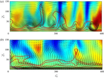
Vector plots of $(v,w)$ in the cross-section ( $y$ – $z$ ) plane located at $x=L_{x}/2$ in figure 14 for (a,b) $M_{b}=0.3$ , (c,d) $M_{b}=0.8$ and (e,f) $M_{b}=1.5$ . (a,c,e) Uncontrolled and (b,d,f) controlled cases with $T^{+}=150$ . The red (dark) and blue (light) correspond to positive and negative streamwise velocity fluctuations. The red lines represent the iso-contours of the streamwise velocity $u=[0.2~0.4~0.6~0.8]U_{b}$ .

The flow field difference among three different $M_{b}$ cases is further examined through the velocity vectors in the cross-section ( $y$ – $z$ ) plane, along with the streamwise velocity fluctuations $u^{\prime }$ , in figure 15. The near-wall quasi-streamwise vortices eject low-speed fluid away from the wall and sweep high-speed fluid towards the wall; note that the effects of shear stress decreasing ejection and shear stress increasing sweep events are unequal, the latter dominating, hence the net effect being increased skin friction by the vortices (Schoppa & Hussain Reference Schoppa and Hussain2002). The streak spacing continuously increases as $M_{b}$ increases. For example, compared with five complete streaks identified in the region with a spanwise length of $600$ wall units at $M_{b}=0.3$ , there are only three streaks at $M_{b}=1.5$ , which is qualitatively consistent with the mean streak spacing of $\unicode[STIX]{x1D706}_{z}^{+}\approx 175$ found from the pre-multiplied energy spectrum in figure 13. Morinishi et al. (Reference Morinishi, Tamano and Nakabayashi2004) and Patel et al. (Reference Patel, Peeters, Boersma and Pecnik2015) also showed that the semi-local scaling could be sufficient to account for the changes in the scales of streak in the buffer layer, to be discussed in § 4.3. Additionally, the streak strength (typically quantified by the streak flank angle) is reduced by SWO. In other words, the streak becomes more stable for high $M_{b}$ cases, which is reasonable since the streamwise vortices have more difficulty in ejecting fluid from the wall as both the density and viscosity increase near the wall. This is also consistent with the attenuation of wall-normal velocity fluctuations at higher $M_{b}$ discussed in § 3.5. SWO significantly weakens the near-wall streaks. Not only the number of streaks but also the streak flank angle is decreased compared with the uncontrolled case. The weakening effect is enhanced as $M_{b}$ increases since the near-wall density and viscosity are further increased due to SWO. In particular, only one complete streak is observed for the $M_{b}=1.5$ case. The weakened streaks lead to the suppression of the generation of streamwise vortices through streak instability/transient growth (Schoppa & Hussain Reference Schoppa and Hussain2002) – resulting in drag reduction.

3.8 Amplitude effect at $Re_{b}=3000$

To further examine the amplitude effect, additional DNS are performed at two other oscillation amplitudes $A^{+}=6$ and $18$ for the $M_{b}=1.5$ case. Figure 5(b) shows the drag reduction ${\mathcal{D}}{\mathcal{R}}$ as a function of $T^{+}$ for different $A^{+}$ values. Consistent with the observations for incompressible flow (Quadrio & Ricco Reference Quadrio and Ricco2004), at given $T^{+}$ , ${\mathcal{D}}{\mathcal{R}}$ increases with $A^{+}$ , but the rate of increase decreases as $A^{+}$ becomes large. Similar to the $A^{+}=12$ case, ${\mathcal{D}}{\mathcal{R}}$ monotonically increases with $T^{+}$ at $A^{+}=18$ , and changes rapidly at $T^{+}=300$ , where the flow is relaminarized (evident from the time evolution of skin friction in figure 16). For the small-amplitude case $A^{+}=6$ , ${\mathcal{D}}{\mathcal{R}}$ exhibits the traditional non-monotonic variation with $T^{+}$ , with ${\mathcal{D}}{\mathcal{R}}_{max}=33.9\,\%\pm 0.8\,\%$ obtained at $T^{+}=200$ .

Figure 16.

Time evolution of skin friction normalized by the uncontrolled case $C_{f}/C_{f,0}$ at $T^{+}=300$ and different $A^{+}$ for $Re_{b}=3000$ and $M_{b}=1.5$ .

Figure 16 shows the long-time evolution of normalized skin friction $C_{f}/C_{f,0}$ at $T^{+}=300$ . For the low-amplitude case $A^{+}=6$ , skin friction exhibits similar behaviour to that shown previously: $C_{f}$ reaches the low-drag state after transients and exhibits small fluctuations due to the turbulence response of wall actuation. For the $A^{+}=12$ case, $C_{f}$ experiences large oscillation before slowly reaching a steady state. For the $A^{+}=18$ case, $C_{f}$ slowly converges to a constant value without large fluctuation, which is about $33.6\,\%$ of $C_{f,0}$ , suggesting that the flow is relaminarized. It is worth mentioning that a similar relaminarization was also observed for drag control using travelling wave-like wall deformation method (Nakanishi et al. Reference Nakanishi, Mamori and Fukagata2012). The initial, periodic large $C_{f}$ oscillations for the $A^{+}=12$ case and the complete relaminarization for $A^{+}=18$ case are quite surprising. As suggested by one referee, these might be due to the limited domain size effect. To address this issue, in the Appendix, we conduct additional simulations for these two cases by doubling the domain length and width. For $A^{+}=18$ , the flow also relaminarizes for the doubled domain size case with identical $C_{f}$ variation. However, for $A^{+}=12$ , we do find an interesting difference: the initial transient period of large $C_{f}$ oscillations becomes shorter, and $C_{f}$ reaches a steady state earlier than for the smaller domain size case. These results seem to suggest that the domain sizes indeed have some influence on the flow transitional behaviour (possibly also relaminarizaiton). Alternation of such large $C_{f}$ oscillations due to domain size variation was also reported in stably stratified turbulent channel flows (Garg et al. Reference Garg, Ferziger, Monismith and Koseff2000; Armenio & Sarkar Reference Armenio and Sarkar2002; Iida, Kasagi & Nagano Reference Iida, Kasagi and Nagano2002; Garcia-Villalba & Del Alamo Reference Garcia-Villalba and Del Alamo2011). Elaborate analysis needs to be carried out to fully understand the possible reasons for transition and relaminarization and the underlining flow physics, which is beyond the scope of this paper.

Interesting, even for the relaminarized case, $C_{f}$ experiences periodic undulation, which is in contrast to the incompressible case, where $C_{f}$ remains constant. To address this, phase-averaged Reynolds shear stress is examined. Combining the phase and Favre averaging, an instantaneous velocity can be expressed as

(3.7) $$\begin{eqnarray}\unicode[STIX]{x1D719}=\check{\unicode[STIX]{x1D719}}(y,\unicode[STIX]{x1D70F})+\unicode[STIX]{x1D719}^{\prime \prime \prime }(x,y,z,t),\end{eqnarray}$$

where $\check{\unicode[STIX]{x1D719}}$ is called phase Favre averaging with random fluctuation $\unicode[STIX]{x1D719}^{\prime \prime \prime }$ defined as

(3.8) $$\begin{eqnarray}\displaystyle & \displaystyle \check{\unicode[STIX]{x1D719}}=\langle \unicode[STIX]{x1D70C}\unicode[STIX]{x1D719}\rangle /\langle \unicode[STIX]{x1D70C}\rangle , & \displaystyle\end{eqnarray}$$

(3.9) $$\begin{eqnarray}\displaystyle & \displaystyle \unicode[STIX]{x1D719}^{\prime \prime \prime }=\unicode[STIX]{x1D719}-\check{\unicode[STIX]{x1D719}}. & \displaystyle\end{eqnarray}$$

The phase-Favre-averaged quantity is further decomposed into time-averaged and periodic components as follows:

(3.10) $$\begin{eqnarray}\check{\unicode[STIX]{x1D719}}(y,\unicode[STIX]{x1D711})=\widetilde{\unicode[STIX]{x1D719}}(y)+\hat{\unicode[STIX]{x1D719}}(y,\unicode[STIX]{x1D711}),\end{eqnarray}$$

so that the instantaneous field can be written in the triple decomposed form as

(3.11) $$\begin{eqnarray}\unicode[STIX]{x1D719}=\widetilde{\unicode[STIX]{x1D719}}(y)+\hat{\unicode[STIX]{x1D719}}(y,\unicode[STIX]{x1D711})+\unicode[STIX]{x1D719}^{\prime \prime \prime }(x,y,z,t),\end{eqnarray}$$

with $\unicode[STIX]{x1D719}^{\prime \prime }=\hat{\unicode[STIX]{x1D719}}+\unicode[STIX]{x1D719}^{\prime \prime \prime }$ .

The phase-averaged Reynolds shear stress can be expressed as

(3.12) $$\begin{eqnarray}\langle \unicode[STIX]{x1D70C}u^{\prime \prime }v^{\prime \prime }\rangle =\langle \unicode[STIX]{x1D70C}(\hat{u} +u^{\prime \prime \prime })(\hat{v}+v^{\prime \prime \prime })\rangle =\hat{u} \langle \unicode[STIX]{x1D70C}v\rangle ,\end{eqnarray}$$

where $u^{\prime \prime \prime }=v^{\prime \prime \prime }=0$ for laminar flow is used. For the incompressible case, based on continuity, $\langle \unicode[STIX]{x1D70C}v\rangle \equiv 0$ , hence $\langle \unicode[STIX]{x1D70C}u^{\prime \prime }v^{\prime \prime }\rangle \equiv 0$ . However, this is no longer valid for compressible flow. From the phase-averaged continuity equation, we have

(3.13) $$\begin{eqnarray}\frac{\unicode[STIX]{x2202}\langle \unicode[STIX]{x1D70C}\rangle }{\unicode[STIX]{x2202}t}+\frac{\unicode[STIX]{x2202}\langle \unicode[STIX]{x1D70C}v\rangle }{\unicode[STIX]{x2202}y}=0.\end{eqnarray}$$

Due to the periodic variation of phase-averaged density $\langle \unicode[STIX]{x1D70C}\rangle$ , $\langle \unicode[STIX]{x1D70C}v\rangle$ is no longer zero, so is $\langle \unicode[STIX]{x1D70C}u^{\prime \prime }v^{\prime \prime }\rangle$ .

Figure 17.

Comparison between (a) phase-wise averaged skin friction $\langle C_{f}\rangle$ , (b) $\langle \unicode[STIX]{x1D70C}v\rangle$ , (c) $\langle \unicode[STIX]{x1D70C}u^{\prime \prime }v^{\prime \prime }\rangle$ and (d) $\text{d}\langle \unicode[STIX]{x1D70C}w\rangle /\text{d}y$ for the relaminarized case ( $A^{+}=18$ and $T^{+}=300$ ) for $Re_{b}=3000$ and $M_{b}=1.5$ . Dashed and dash-dotted vertical lines denote locations of the minimum and maximum of $\langle C_{f}\rangle$ , respectively.

Figure 17 shows, for the relaminarized case, the phase-averaged skin-friction distribution $\langle C_{f}\rangle$ , along with $\langle \unicode[STIX]{x1D70C}v\rangle$ , Reynolds shear stress $\langle \unicode[STIX]{x1D70C}u^{\prime \prime }v^{\prime \prime }\rangle$ and $\text{d}\langle \unicode[STIX]{x1D70C}w\rangle /\text{d}y$ denoting the Stokes strain. The skin friction $\langle C_{f}\rangle$ varies within the cycling phase $\unicode[STIX]{x1D711}$ with the oscillation period of half the SWO period. Additionally, $\langle \unicode[STIX]{x1D70C}v\rangle$ also varies with $\unicode[STIX]{x1D711}$ and with maximum variation located around $y/h=-0.9$ . Consequently, the Reynolds shear stress $\langle \unicode[STIX]{x1D70C}u^{\prime \prime }v^{\prime \prime }\rangle$ also varies periodically with $\unicode[STIX]{x1D711}$ . Consistent with the observation made in Touber & Leschziner (Reference Touber and Leschziner2012), figure 17 shows that the skin friction is also related to the Stokes strain: $\langle C_{f}\rangle$ rises when the Stokes strain near the wall is high while it decreases when the strain is low. Hence, due to the periodic variation of the thermodynamic quantities caused by SWO, even for the laminar case the motions in the streamwise and spanwise directions are coupled. This is in contrast to the incompressible flow, where these two flows can be decoupled. The periodical variation of thermodynamic properties is also the reason why skin friction $C_{f}$ experiences strong oscillations at small $T^{+}$ for the $M_{b}=1.5$ case (figure 4 c).

The decomposed total skin-friction drag for different $T^{+}$ is shown in figure 18. Again, $C_{f}^{T}$ is the dominant term for the reduction of total $C_{f}$ . For the relaminarized case ( $A^{+}=18$ and $T^{+}=300$ ), the turbulence contribution $C_{f}^{T}$ becomes zero. Not surprisingly, the existence of compressible part $C_{f}^{\unicode[STIX]{x1D707}}$ due to non-uniform thermodynamic properties causes the skin friction for the relaminarized compressible flow to be slightly higher than that for the well-known incompressible laminar cases. Due to increased viscosity near the wall caused by increased temperature, the compressible contribution $C_{f}^{\unicode[STIX]{x1D707}}$ continuously increases with $A^{+}$ . For example, at $T^{+}=25$ , $C_{f}^{\unicode[STIX]{x1D707}}/C_{f,0}$ markedly increases from approximately $4.9\,\%$ at $A^{+}=6$ to $8.1\,\%$ at $A^{+}=18$ . This suggests that ${\mathcal{D}}{\mathcal{R}}$ might be decreased at very high $A^{+}$ , due to enhanced compressibility contribution $C_{f}^{\unicode[STIX]{x1D707}}$ . This is quite different from the incompressible case, where ${\mathcal{D}}{\mathcal{R}}$ monotonically increases with $A^{+}$ (figure 5 b; see also Quadrio & Ricco (Reference Quadrio and Ricco2004)).

Figure 18.

Decomposed skin friction $C_{f}$ for different oscillating period $T^{+}$ at (a) $A^{+}=6$ and (b) $A^{+}=18$ for $Re_{b}=3000$ and $M_{b}=1.5$ .

4.1 Reynolds number effect

Figure 19.

Initial time evolution ( $t^{+}\leqslant 7000$ ) of skin friction normalized by the uncontrolled case $C_{f}/C_{f,0}$ at different wall oscillation periods $T^{+}$ with $A^{+}=12$ for $Re_{b}=7667$ and (a) $M_{b}=0.8$ and (b) $M_{b}=1.5$ .

Since the Reynolds number effect is an important issue for drag control, we performed additional studies at a higher $Re_{b}=7667$ for the subsonic $M_{b}=0.8$ and supersonic $M_{b}=1.5$ cases (denoted as C8kM08 and C8kM15 cases, respectively). Figure 19 shows the initial time evolution of the normalized skin friction coefficient $C_{f}(t)/C_{f,0}$ for different oscillation periods $T^{+}$ with $A^{+}=12$ at $Re_{b}=7667$ . In general, the evolution of $C_{f}(t)$ has a similar pattern to that at $Re_{b}=3000$ (figure 4), namely $C_{f}(t)$ initially rapidly decreases as the oscillation starts, then reaches a temporal minimum before approaching the statistically quasi-steady, low-drag state. However, compared with the results at $Re_{b}=3000$ , the long-time-scale undulation of $C_{f}$ is suppressed, especially for the large $T^{+}$ cases. This suggests that the rapid increase and decrease of $C_{f}$ for $Re_{b}=3000$ and $M_{b}=1.5$ might be due to a low Reynolds number effect. In addition, at the same $T^{+}$ , the level of small-scale oscillation in $C_{f}$ (indicating the flow responses to wall oscillation) is found to increase as $Re_{b}$ increases, akin to the observation of Hurst et al. (Reference Hurst, Yang and Chung2014) for the strictly incompressible case.

Figures 20(a) and 20(b) show ${\mathcal{D}}{\mathcal{R}}$ as a function of $T^{+}$ at $A^{+}=12$ at two different $Re_{b}$ values for the $M_{b}=0.8$ and $1.5$ cases, respectively. It can be seen that ${\mathcal{D}}{\mathcal{R}}$ clearly decreases at higher $Re_{b}$ , akin to the incompressible drag control using SWO (Gatti & Quadrio Reference Gatti and Quadrio2016; Hurst et al. Reference Hurst, Yang and Chung2014) as well as many other drag methods (Wang, Huang & Xu Reference Wang, Huang and Xu2016; Yao, Chen & Hussain Reference Yao, Chen and Hussain2018). The rate of decrease strongly depends on the oscillation period $T^{+}$ : ${\mathcal{D}}{\mathcal{R}}$ changes less at small $T^{+}$ (large $\unicode[STIX]{x1D714}^{+}$ ), but much more at large $T^{+}$ . If assuming that drag reduction decreases with Reynolds number following ${\mathcal{D}}{\mathcal{R}}\propto Re_{\unicode[STIX]{x1D70F}}^{-\unicode[STIX]{x1D6FE}}$ , the scaling exponent $\unicode[STIX]{x1D6FE}$ for the $M_{b}=0.8$ case increases from $0.1$ for $T^{+}=25$ to $0.49$ for $T^{+}=300$ (a large $\unicode[STIX]{x1D6FE}$ denotes a rapid decrease in ${\mathcal{D}}{\mathcal{R}}$ with increasing Reynolds number). In particular, ${\mathcal{D}}{\mathcal{R}}$ at $T^{+}=150$ has been reduced from $37.6\,\%\pm 1.1\,\%$ to $29.3\,\%\pm 1.1\,\%$ , which corresponds to $\unicode[STIX]{x1D6FE}=0.29$ (close to the value of $0.35$ obtained by Yao et al. (Reference Yao, Chen and Hussain2019) for the incompressible case at the same $T^{+}$ ). Consistent with the finding for incompressible flow (Hurst et al. Reference Hurst, Yang and Chung2014; Yao et al. Reference Yao, Chen and Hussain2019), the optimal period $T^{+}$ also seems to decrease with increasing $Re_{b}$ , i.e. from $T_{opt}^{+}=150$ at $Re_{b}=3000$ to $T_{opt}^{+}=100$ at $Re_{b}=7667$ (with ${\mathcal{D}}{\mathcal{R}}_{max}=30.3\,\%\pm 0.8\,\%$ ). For $M_{b}=1.5$ , ${\mathcal{D}}{\mathcal{R}}$ becomes non-monotonically changing with $T^{+}$ at $Re_{b}=7667$ , with ${\mathcal{D}}{\mathcal{R}}_{max}$ of $33.7\,\%\pm 0.6\,\%$ obtained at $T^{+}=150$ . Figure 20(b) shows that the decrease in ${\mathcal{D}}{\mathcal{R}}$ with Reynolds number is more severe for $M_{b}=1.5$ . However, recall that the drag control at $Re_{b}=3000$ suffers from the low Reynolds number effect, where the flow does not remain fully developed at large $T^{+}$ . Hence, inferring any Reynolds number scaling from those two cases can be limiting.

Figure 20.

Reynolds number dependence of drag reduction ${\mathcal{D}}{\mathcal{R}}$ versus oscillation period $T^{+}$ at $A^{+}=12$ for (a) $M_{b}=0.8$ and (b) $M_{b}=1.5$ . The error bars indicate the corresponding uncertainty of ${\mathcal{D}}{\mathcal{R}}$ .

Figure 21.

Comparison of Trettel–Larsson transformed mean streamwise velocity $U^{\ast }$ as a function of $y^{\ast }$ between uncontrolled and controlled at $T^{+}=150$ for C3kM15 and C8kM15 cases.

Flow statistics for $M_{b}=1.5$ are compared between two different $Re_{b}$ cases at the near-optimal control period (i.e. $T^{+}=150$ ). The mean velocity profiles using Trettel–Larsson transformation ( $U^{\ast }$ ) are displayed in figure 21 for both uncontrolled and controlled cases at $M_{b}=1.5$ with $Re_{b}=3000$ and $Re_{b}=7667$ . For the uncontrolled case, the Trettel–Larsson transformed mean velocity profiles agree with the log-law profile, especially for the $Re_{b}=7667$ case. When scaled with the actual friction velocity, the mean velocity profiles for the controlled flow collapse with those of uncontrolled cases in the viscous sublayer and are shifted upward in the log region. The shift decreases as $Re_{b}$ increases, which is consistent with the findings for incompressible flows (Hurst et al. Reference Hurst, Yang and Chung2014; Yao et al. Reference Yao, Chen and Hussain2019). Gatti & Quadrio (Reference Gatti and Quadrio2016) proposed a model to characterize ${\mathcal{D}}{\mathcal{R}}$ via the vertical shift of the mean velocity profile. By further assuming that the upward shift would become invariant at high $Re$ , they further employed this model to predict the possible amount of ${\mathcal{D}}{\mathcal{R}}$ at practical Reynolds numbers. If this assumption is also valid for the compressible cases, it might be interesting to extend that to include the $M_{b}$ effect, with the aid of certain mean velocity transformations, like van Driest or Trettel–Larsson transformations.

Figure 22.

Comparison of Reynolds stress $\unicode[STIX]{x1D70F}_{ij}$ profiles between uncontrolled and controlled at $T^{+}=150$ for C3kM15 and C8kM15 cases: (a) $\unicode[STIX]{x1D70F}_{11}$ , (b) $\unicode[STIX]{x1D70F}_{22}$ , (c) $\unicode[STIX]{x1D70F}_{33}$ and (d) $\unicode[STIX]{x1D70F}_{12}$ . See figure 21 for description of the curves.

Figure 22 further shows the Reynolds stresses ( $\unicode[STIX]{x1D70F}_{11}$ , $\unicode[STIX]{x1D70F}_{22}$ , $\unicode[STIX]{x1D70F}_{33}$ and $\unicode[STIX]{x1D70F}_{12}$ ) at $Re_{b}=3000$ and $7667$ for $M_{b}=1.5$ . In general, all Reynolds stresses are significantly suppressed under SWO, and the location for the peak moves away from the wall. The decreases are much more substantial at lower $Re_{b}$ . As $Re_{b}$ increases, the effects of control on the Reynolds stresses become weaker. Taking $\unicode[STIX]{x1D70F}_{11}$ for example, the maximum peak slightly increases for the uncontrolled case when $Re_{b}$ increases from $3000$ to $7667$ , but the difference between the two peaks becomes larger under control. In addition, the difference between the peak locations of the uncontrolled and controlled cases also decreases with increasing $Re_{b}$ . All these findings show that SWO becomes less effective in suppressing turbulent fluctuations as $Re_{b}$ increases, which explains why ${\mathcal{D}}{\mathcal{R}}$ deteriorates at high Reynolds numbers (also valid for incompressible cases).

Figure 23.

Pre-multiplied spanwise spectrum of streamwise velocity $k_{z}E_{uu}$ (normalized by the maximum value of uncontrolled case) as a function of $\unicode[STIX]{x1D706}_{z}^{+}$ for C8kM15 for (a) uncontrolled and (b) controlled cases with $T^{+}=150$ .

Figure 23 compares the pre-multiplied spanwise wavenumber spectrum of streamwise velocity $k_{z}E_{uu}$ (normalized by the maximum value of uncontrolled case) for both uncontrolled and controlled cases with $T^{+}=150$ . Compared with $Re_{b}=3000$ , the energy-containing part enlarges as $Re_{b}$ increases. However, the peak location only varies slightly compared with the $Re_{b}=3000$ case, which becomes $\unicode[STIX]{x1D706}_{z}^{+}\approx 179$ at $y^{+}\approx 19.2$ . Similar to the low $Re_{b}$ cases, the intensity becomes weaker under control and the wall-normal location of the peak increases. However, compared with that at $Re_{b}=3000$ (figure 13 f), $k_{z}E_{uu}$ becomes less attenuated near the wall (i.e. $y^{+}\lesssim 20$ ), suggesting less effectiveness of control.

Figure 24.

Top view of instantaneous vortical structures (visualized using $\unicode[STIX]{x1D706}_{\unicode[STIX]{x1D70C}}^{+}$ ) associated with the streamwise velocity fluctuations (streaks) $|u^{\prime }/U_{b}|<0.4$ at $y^{+}\approx 15$ at C8kM15 for (a) uncontrolled and (b) controlled cases with $T^{+}=150$ . The red (dark) and blue (light) correspond to positive and negative fluctuations. Note that the domain size is $L_{x}\times L_{z}=6\unicode[STIX]{x03C0}h\times 2\unicode[STIX]{x03C0}h$ , and the black dashed box corresponds to the same domain size as in figure 14 in wall units.

The instantaneous vortical structures visualized using $\unicode[STIX]{x1D706}_{\unicode[STIX]{x1D70C}}$ criterion, along with the streaks at $y^{+}\approx 15$ , are shown in figure 24 for both the uncontrolled and controlled cases for $Re_{b}=7667$ and $M_{b}=1.5$ . Note that the black box in figure 24 indicates the same domain size as in figure 14(e,f) in wall units. For the uncontrolled case, vortices are clustered in the region of large-scale low-speed streaks. Although both the low-speed streaks and the near-wall streamwise vortices are suppressed under control, the suppression becomes less effective compared with the cases at $Re_{b}=3000$ . Figure 25 further displays the velocity vectors in the cross-section ( $y$ – $z$ ) plane at the middle of the streamwise domain, along with the streamwise velocity fluctuations $u^{\prime }$ . At the flank of the low-speed streak, several near-wall quasi-streamwise vortices exist, ejecting/sweeping low-/high-speed fluid from/to the wall. Compared with those at $Re_{b}=3000$ (figure 14 e), these vortices becomes stronger. Under control, the streak becomes significantly weakened, especially very close to the wall. Interestingly, at this particular streamwise location, we capture one event of streak break up, which is caused by the squeezing and ejection motions of counter-rotating vortex pairs.

Figure 25.

Vector plots of $(v,w)$ in the $y$ – $z$ plane located at $x=L_{x}/2$ in figure 24 for C8kM15 case. (a) Uncontrolled and (b) controlled cases at $T^{+}=150$ . The red (dark) and blue (light) correspond to positive and negative streamwise velocity fluctuations. The red lines represent the iso-contours of the streamwise velocity $u=[0.2~0.4~0.6~0.8]U_{b}$ .

4.2 Comparison with incompressible case at comparable semi-local Reynolds number

Previous work on CTCF revealed that semi-local scaling can be employed to derive transformations that better collapse the mean velocity and turbulent statistics between incompressible and compressible cases (Huang et al. Reference Huang, Coleman and Bradshaw1995; Modesti & Pirozzoli Reference Modesti and Pirozzoli2016; Patel et al. Reference Patel, Boersma and Pecnik2016). Figure 26 shows the mean velocity profiles using the Trettel–Larsson transformation and the Reynolds stresses as a function of $y^{\ast }$ for two different $Re_{b}$ values at $M_{b}=1.5$ . Two incompressible cases at matching $Re_{\unicode[STIX]{x1D70F}c}^{\ast }$ , namely $140$ and $340$ , are also included for comparison. (Here, $Re_{\unicode[STIX]{x1D70F}c}^{\ast }$ indicates the semi-local Reynolds number $Re_{\unicode[STIX]{x1D70F}}^{\ast }$ at the half-channel centre height.) Clearly, the transformed mean velocity profiles are in good congruence with the incompressible cases. In addition, the semi-local scaling also yields good collapses for the Reynolds stresses. In particular, the wall-normal, spanwise and shear stresses are almost perfectly matched, and the peak locations of streamwise Reynolds stress occur at similar $y^{\ast }$ , i.e. around $15$ . The only apparent difference is that the peak of the streamwise Reynolds stress is slightly larger for the supersonic cases. Patel et al. (Reference Patel, Peeters, Boersma and Pecnik2015) found that the enhancement of the peak is related to the strengthening of the large-scale components of the streamwise velocity in the buffer layer.

Figure 26.

(a) Trettel–Larsson transformed mean velocity and (b) Reynolds stresses for the compressible C3kM15 and C8kM15 cases, along with the strictly incompressible cases at $Re_{\unicode[STIX]{x1D70F}}=140$ and $340$ .

Figure 27.

Pre-multiplied spanwise spectrum of streamwise velocity $k_{z}E_{uu}$ (normalized by the maximum value of uncontrolled case) in semi-local units for (a) C6kM00 and (b) C8kM15 cases.

Figure 27 further compares the pre-multiplied spanwise spectrum of streamwise velocity $k_{z}E_{uu}$ for the supersonic ( $Re_{b}=7667$ and $M_{b}=1.5$ ) and the incompressible $Re_{\unicode[STIX]{x1D70F}}=340$ cases in semi-local units. Compared with figure 23(a), which shows the same quantity in wall units, the pre-multiplied spanwise spectrum of streamwise velocity in semi-local units better resembles that of the incompressible $Re_{\unicode[STIX]{x1D70F}}=340$ case. The mean-streak spacing, indicated by the peak location, becomes $\unicode[STIX]{x1D706}_{z}^{\ast }\approx 120$ at $y^{\ast }=15$ , which is the same as for the incompressible case. Figure 28 further shows the instantaneous streamwise velocity fluctuations in the $x$ – $z$ plane at $y^{\ast }=15$ for these two cases. For the supersonic case, representations in both classical wall units ( $x^{+}=xRe_{\unicode[STIX]{x1D70F}}$ ) and semi-local units ( $x^{\ast }=xRe_{\unicode[STIX]{x1D70F}}^{\ast }$ ) are shown. The box size in streamwise and spanwise directions is $4000\times 2000$ , based on corresponding non-dimensional coordinates $x^{+}\times z^{+}$ / $x^{\ast }\times z^{\ast }$ . In order to outline the physical scale of the structures, the black box in figure 28(c) indicates the domain of figure 28(b). Similar to the previous findings, the streaks become longer and sparse in wall units. However, when scaled in the same local units, mean spanwise spacing and length of the streaks become similar between the supersonic and incompressible cases. Patel et al. (Reference Patel, Boersma and Pecnik2016) also showed that the mean streak spacing, when scaled in semi-local units, is nearly universal for $y^{\ast }>12$ . Chen et al. (Reference Chen, Hussain, Pei and She2014) also found that the wall-normal location of the induced vorticity–velocity correlation structures is quite universal in semi-local units for different $M_{b}$ values.

Figure 28.

Instantaneous streamwise velocity fluctuations in the $x$ – $z$ plane at $y^{\ast }=15$ for (a) I6kM00 case, (b) C8kM15 case using $x^{+}$ – $z^{+}$ coordinates and (c) C8kM15 case using $x^{\ast }$ – $z^{\ast }$ coordinates. Note that the black box in (c) corresponds to (b).

All the above results demonstrate that there is a strong similarity between compressible and incompressible flows at matching $Re_{\unicode[STIX]{x1D70F}c}^{\ast }$ . Hence, it is interesting to investigate and compare drag control performance at comparable $Re_{\unicode[STIX]{x1D70F}c}^{\ast }$ . Figure 29(a) compares ${\mathcal{D}}{\mathcal{R}}$ as a function of $T^{+}$ at $A^{+}=12$ between the supersonic $M_{b}=1.5$ (with $Re_{b}=3000$ and $7667$ ) and the incompressible ( $Re_{\unicode[STIX]{x1D70F}}=140$ and $340$ ) cases. Similar to figure 5, the optimal oscillation period $T_{opt}^{+}$ becomes large for the supersonic cases. Based on our observation that the length scale increases with $M_{b}$ when scaled in wall units and can match well when scaled in semi-local units, we propose a simple transformation to better collapse ${\mathcal{D}}{\mathcal{R}}$ between incompressible and compressible cases. For a given oscillation period $T^{+}$ and amplitude $A^{+}$ , the control can also be described by another parameter, namely its maximum displacement $D$ , which is $D=AT/\unicode[STIX]{x03C0}$ for the sinusoidal oscillation case. Now, let us assume that at the same $Re_{\unicode[STIX]{x1D70F}c}^{\ast }$ , the length scale of the forcing is correlated with the mean streak spacing of the flow, then we have

(4.1) $$\begin{eqnarray}\frac{D^{\ast }}{l^{\ast }}=\frac{D_{I}^{+}}{l_{I}^{+}}=\frac{D_{C}^{+}}{l_{C}^{+}},\end{eqnarray}$$

where $I$ and $C$ denote the length scale for the incompressible and compressible cases, respectively, and $l^{\ast }$ and $D^{\ast }$ are the normalized length scale for the streak and control. Moreover, we have $l^{\ast }=l_{I}^{+}$ . For the same oscillation amplitude $A^{+}$ , we can obtain a normalized oscillation period as

(4.2) $$\begin{eqnarray}T^{\ast }=T_{I}^{+}=T_{C}^{+}\frac{l_{I}^{+}}{l_{C}^{+}}.\end{eqnarray}$$

Figure 29(b) shows ${\mathcal{D}}{\mathcal{R}}$ as a function of $T^{\ast }$ for supersonic and incompressible cases. Compared with figure 29(a), ${\mathcal{D}}{\mathcal{R}}$ agrees better between these cases, except that ${\mathcal{D}}{\mathcal{R}}$ is slightly higher for the supersonic case – this seems understandable since the streaks are more coherent and stable in the supersonic case. This is even true for flow under SWO, where the density and viscosity are further increased near the wall. Figure 29(c) further shows ${\mathcal{D}}{\mathcal{R}}$ normalized by the maximum value for the supersonic $M_{b}=1.5$ with $Re_{b}=7667$ and incompressible $Re_{\unicode[STIX]{x1D70F}}=340$ cases (note that due to monotonic increase for the $Re_{b}=3000$ case, the two low-Reynolds-number cases are not included for comparison). Clearly, ${\mathcal{D}}{\mathcal{R}}$ shows a better collapse, especially at small $T^{\ast }$ . The optimal $T_{opt}^{\ast }$ , which is around $100$ , seems to be $M_{b}$ -invariant.

Figure 29.

Comparison of ${\mathcal{D}}{\mathcal{R}}\,(\%)$ for different cases (C3kM15, C8kM15, I2kM00 and I6kM00) at $A^{+}=12$ as a function of (a) $T^{+}$ and (b) $T^{\ast }$ . (c) Values of ${\mathcal{D}}{\mathcal{R}}$ normalized by the maximum as a function of $T^{\ast }$ for C8kM15 and I6kM00 cases. The error bars in (a,b) indicate the corresponding uncertainty of ${\mathcal{D}}{\mathcal{R}}$ .

Figure 30(a,b) compares the mean velocity $U^{\ast }$ and Reynolds shear stress $\unicode[STIX]{x1D70F}_{12}$ between the supersonic $Re_{b}=7677$ and incompressible $Re_{\unicode[STIX]{x1D70F}}=340$ cases near $T_{opt}^{\ast }$ (corresponding to $T^{+}=100$ for the incompressible $Re_{\unicode[STIX]{x1D70F}}=340$ and $T^{+}=150$ for the supersonic $Re_{b}=7677$ cases, respectively). Except for a slightly larger upward shift associated with higher ${\mathcal{D}}{\mathcal{R}}$ , the mean velocity profiles under control are well collapsed between these two cases. In addition, the Reynolds shear stress also shows good congruence. Figure 30(c) further shows decomposed skin friction $C_{f}$ for these two different cases. For the incompressible, uncontrolled case, the decomposition only contains laminar $C_{f}^{L}$ and turbulent contributions $C_{f}^{T}$ , amounting to about $15.1\,\%$ and $84.9\,\%$ , respectively. Under control, the turbulent contribution $C_{f}^{T}$ decreases to approximately $54.7\,\%$ . For the supersonic case, the laminar $C_{f}^{L}$ and compressible $C_{f}^{\unicode[STIX]{x1D707}}$ parts contribute about $12.2\,\%$ and $2.1\,\%$ , respectively, and the turbulent contribution $C_{f}^{T}$ is approximately $85.5\,\%$ . Under control, the compressible part $C_{f}^{\unicode[STIX]{x1D707}}$ increases by approximately $0.3\,\%$ , while the turbulent part $C_{f}^{T}$ decreases to about $51.6\,\%$ of $C_{f,0}$ , resulting in a total $3.3\,\%$ more ${\mathcal{D}}{\mathcal{R}}$ for the supersonic case. It is also worth mentioning that as $Re_{b}$ increases, the contributions from laminar $C_{f}^{L}$ and compressible $C_{f}^{\unicode[STIX]{x1D707}}$ parts decrease, and that from the turbulent part $C_{f}^{T}$ monotonically increases, which suggests that at high Reynolds numbers the suppression of the turbulent Reynolds shear stress is still the primary objective of drag control for supersonic flows.

Figure 30.

Comparison of (a) Trettel–Larsson transformed mean velocity $U^{\ast }$ , (b) Reynolds shear stress $\unicode[STIX]{x1D70F}_{12}$ and (c) decomposed skin friction $C_{f}$ between uncontrolled and near-optimal controlled cases for C8kM15 and I6kM00.

Figure 31.

Comparison of pre-multiplied spanwise spectra between uncontrolled and near-optimal controlled cases for C8kM15 and I6kM00 for (a) streamwise Reynolds stress $k_{z}E_{uu}/u_{\unicode[STIX]{x1D70F}}^{2}$ and (b) Reynolds shear stress $k_{z}E_{uv}/u_{\unicode[STIX]{x1D70F}}^{2}$ as a function of $\unicode[STIX]{x1D706}_{z}^{\ast }$ at the peak wall-normal locations $y^{\ast }\approx 15$ and $25$ , respectively.

The response of the motions at different scales to the control is further discussed with the pre-multiplied wavenumber spectrum of the Reynolds stresses. Figure 31(a) compares the pre-multiplied spanwise wavenumber spectrum of the streamwise Reynolds stress $k_{z}E_{uu}/u_{\unicode[STIX]{x1D70F}}^{2}$ as a function of wavelength $\unicode[STIX]{x1D706}_{z}^{\ast }$ at $y^{\ast }=15$ for the above cases. As discussed, the spectrum for the uncontrolled case displays a distinct peak, approximately located at $\unicode[STIX]{x1D706}_{z}^{\ast }\approx 120$ and is almost invariant with $M_{b}$ . Compared with the incompressible case, the near-wall large scales are slightly larger for the supersonic case, causing a larger peak of the streamwise Reynolds stress (figure 26 b). Under control, the overall shape of the spectrum is not significantly changed. The Reynolds stress is substantially suppressed at small scales, with the peak reduced to approximately $65\,\%$ of the uncontrolled value. For the supersonic case, the large-scale components are less suppressed compared with the incompressible case, indicating the presence of more large-scale streaks. Figure 31(b) further compares the pre-multiplied spanwise wavenumber spectrum of the Reynolds shear stress $k_{z}E_{uv}$ as a function of wavelength $\unicode[STIX]{x1D706}_{z}^{\ast }$ at $y^{\ast }=25$ . For the uncontrolled cases, the profiles are almost collapsed with a peak around $\unicode[STIX]{x1D706}_{z}^{\ast }\approx 100$ , which is also consistent with the finding in figure 26(b), where the Reynolds shear stress is better matched between the two cases. Here SWO significantly suppresses the stress at all scales. For the incompressible case, the peak under control is decreased to about $61\,\%$ of the uncontrolled one. For the supersonic case, a slightly larger suppression is observed, especially for the small scales (i.e. $\unicode[STIX]{x1D706}_{z}^{\ast }<200$ ), which, in combination of the above FIK analysis, suggests that the slightly higher ${\mathcal{D}}{\mathcal{R}}$ for the supersonic case is due to enhanced effectiveness of suppressing near-wall turbulence.