2.1 Dynamical modelling of the hexarotor

This section derives the equations of motion and attitude dynamics for a hexarotor UAV. Its configuration is represented in Fig. 1. Consider first a body-fixed reference frame R_B with the x_B, y_B, z_B axis originating at the center of mass of the vehicle. The x_B axis points to the front direction, the y_B axis points to the left direction and the z_B axis points upwards. Consider second an inertial frame R_I fixed to the earth {o, x_I, y_I, z_I}.

Figure 1.

The PPNNPN hexarotor configuration.

The equations governing the motion of the system are obtained using the Euler-Lagrange approach and give the commonly used model a hybrid coordinate system, where the vehicle’s center of mass translational dynamics are expressed in the inertial frame and its angular dynamics are expressed in the body frame^{(Reference Bouabdallah19)}:

$$\matrix{ {\ddot x = (\cos \phi \sin \theta \cos \psi + \sin \phi \sin \psi ){{{u_f}} \over m}} \hfill \cr {\ddot y = (\cos \phi \sin \theta \sin \psi - \sin \phi \cos \psi ){{{u_f}} \over m}} \hfill \cr {\ddot z = (\cos \phi \cos \theta ){{{u_f}} \over m} - g} \hfill \cr {\dot p = {{{I_{yy}} - {I_{zz}}} \over {{I_{xx}}}}qr - {{{J_r}} \over {{I_{xx}}}}q\Omega + {1 \over {{I_{xx}}}}{\tau _\phi }} \hfill \cr {\dot q = {{{I_{zz}} - {I_{xx}}} \over {{I_{yy}}}}pr + {{{J_r}} \over {{I_{yy}}}}p\Omega + {1 \over {{I_{yy}}}}{\tau _\theta }} \hfill \cr {\dot r = {{{I_{xx}} - {I_{yy}}} \over {{I_{zz}}}}pq + {1 \over {{I_{zz}}}}{\tau _\psi }} \hfill \cr {} \hfill \cr } $$ (1)

In these equations, x, y and z denote the position of the vehicle and ϕ, θ, and ψ the Euler angles with respect to the earth frame. p, q and r denote the angular velocities of the vehicule with respect to the body frame, I_xx, I_yy, I_zz and J_r are respectively the moments of inertia of the hexarotor on the three axes with respect to R_B and the rotor inertia.τ_ϕ,τ_θ andτ_ψ are the torques inputs around the x_B, y_B and z_B axes. Ω is the overall residual propeller speed from the unbalanced rotor rotation as seen below:

$$\Omega = \sum\limits_{i = 1}^6 {\omega _i}$$ (2)

where ω_i, the i^th propeller speed, is considered as positive or negative depending on the rotation direction of the motor i.

The rotating speed relation between the body coordinates and the inertial coordinates can be written as follows:

$$\left[ {\matrix{ {\dot \phi } \cr {\dot \theta } \cr {\dot \psi } \cr } } \right] = \left[ {\matrix{ 1 \quad {\sin \phi \tan \theta } \quad {\cos \phi \tan \theta } \cr 0 \quad {\cos \phi } \quad { - \sin \phi } \cr 0 \quad {\sin \phi /\cos \theta } \quad {\cos \phi /\cos \theta } \cr } } \right]\left[ {\matrix{ p \cr q \cr r \cr } } \right]$$ (3)

The translational motion of the UAV depends on the total thrust force u_f, which is the sum of the thrust forces of each propeller as seen below:

(4) $${u_f} = \sum\limits_{i = 1}^6 {f_i}$$

where the thrust force of each propeller is denoted by f_i and is directly proportional to the rotational speed of each propeller. The input torques can be related to the propellers thrust forces f_i through:

(5) $$\matrix{ {{\tau _\phi } = l( - {1 \over 2}{f_1} - {f_2} - {1 \over 2}{f_3} + {1 \over 2}{f_4} + {f_5} + {1 \over 2}{f_6})} \hfill \cr {{\tau _\theta } = l({{\sqrt 3 } \over 2}{f_1} - {{\sqrt 3 } \over 2}{f_3} - {{\sqrt 3 } \over 2}{f_4} + {{\sqrt 3 } \over 2}{f_6})} \hfill \cr {{\tau _\psi } = {\tau _1} + {\tau _2} - {\tau _3} + {\tau _4} - {\tau _5} - {\tau _6}} \hfill \cr {} \hfill \cr } $$

with

$$\matrix{ {{f_i} = {K_f}\omega _i^2} \hfill \cr {{\tau _i} = {K_t}\omega _i^2} \hfill \cr {} \hfill \cr } $$ (6)

l is the length of each arm, and K_f and K_t are the thrust and reaction torques coefficients, respectively.

2.2 Control strategy

A control strategy for stabilising the hexarotor while hovering and following trajectories is presented in this section. The hexarotor, having only four control inputs (u_f,τ_ϕ,τ_θ,τ_ψ ) does not allow direct control of all of the degrees of freedom (DOFs). Control of positions x and y is achieved indirectly through control of roll and pitch angles in an outer control loop that analyses sensor data and desired mission data. Its outputs are the desired angle values for the inner control loop, which then controls the roll, pitch and yaw angles (Fig. 2). The outputs of the inner loop are the control variables that stabilise the position error through the four basic movements of the hexarotor.

Figure 2.

The control strategy.

In both loops, states are controlled by proportional-integral-derivative (PID) controllers that make use of information obtained from an inertial measurement unit (IMU) and a global positioning system (GPS):

$$u = {K_p}e + {K_d}\dot e + {K_I}\int_0^t e(\tau )d(\tau )$$ (7)

K_p, K_d and K_I are the controller’s gains, and e is the state error compared to the desired position. A proportional-integral-derivative (PID) controller applied on a multirotor has the advantage of being simple to design with the parameter gains being easy to adjust.

3.1 Faults scenarios

In this paper, it will be assumed that the hexarotor is subject to control effectiveness losses in one or multiple actuators. A loss can be represented by γ_i, where γ_i = 0 and γ_i = 1 indicate, respectively, that the actuator is completely healthy or fully failing. Then the thrust produced by a motor is given by:

$${\bar u_i}(t) = (1 - {\gamma _i}(t)){u_i}(t)$$ (8)

Consider the hexarotor system described by the following state space equation:

$$\matrix{ {\dot X(t)} \hfill \quad { = f(X(t)) + \sum\nolimits_{i = 1}^6 {} {g_i}(X(t)){u_i}(t)} \hfill \cr {} \hfill \quad { = f(X(t)) + G(X(t))u(t)} \hfill \cr {} \hfill \quad {} \hfill \cr } $$ (9)

where X εRⁿ and u = [u ₁ u ₂ … u ₆]^T are the system states and the control input vector (motors speeds in our case). The matrix G is column rank deficient:

$$rank(G) = K < 6\,\,\forall X \in {R^n}$$ (10)

The input signal u(t) belongs to a compact set that is defined as:

$$u(t) \in \Omega \equiv \{ u \in {R^6}|{u^ - } \le u \le {u^ + }\} $$ (11)

where the constraints are defined so that: $${u^ - } \equiv {[0\,\,0\,\,&#x2026;\,\,0]^T}$$ and $${u^ + } \equiv {[{u_{1,max}}\,\,{u_{2,max}}\,\,&#x2026;\,\,{u_{6,max}}]^T}$$.

It will be assumed that the hexarotor system subject to actuators faults can be written as:

$$\dot X(t) = f(X(t)) + Gu(t) - G\gamma u(t)$$ (12)

by defining the effectiveness gain γ matrix as:

$$\matrix{ {\gamma (t) = {\rm{d}}iag({\gamma _1}(t),{\gamma _2}(t),&#x2026;,{\gamma _6}(t))} \hfill \cr {0 \le {\gamma _i}(t) \le 1} \hfill \cr {} \hfill \cr } $$ (13)

The state space equation of system facing actuators faults is given as:

$$\matrix{ {\dot X(t) = f(X(t)) + GWu(t)} \hfill \cr {W(t) = I - \gamma (t)} \hfill \cr {} \hfill \cr } $$ (14)

3.2 Static hovering analysis

A standard hexarotor with alternating rotors cannot be considered as a fail-safe multirotor platform, in spite of the existence of actuators redundancy, when compared to a conventional quadrotor. A PNPNPN hexarotor cannot statically hover with only five rotors. A solution is to consider tilted rotors to guarantee a hover solution in case of actuators failures^{(Reference Michieletto, Ryll and Franchi20)} or to modify the configuration to obtain a PPNNPN hexarotor. An analysis on the existence of static hover solutions based on the multi-parametric programming optimisation and the modified Kalman rank condition is presented below for the PPNNPN hexarotor considered in this paper. The hexarotor is in static hover when its position and attitude are stably kept constant or a solution of the form^{(Reference Michieletto, Ryll and Franchi20)} : u_f = mg,τ_ϕ = 0,τ_θ = 0,τ_ψ = 0 can be found without violating the constraints on the motors speeds. The existence of such solutions can be simply verified by solving a multi-parametric optimisation problem near hovering:

$$\matrix{ {} \hfill \quad {\mathop {\min }\limits_u {1 \over 2}{u^T}u} \hfill \cr {{\rm{s}}uch\,\,{\rm{t}}hat:} \hfill \quad {\left\{ {\matrix{ {{u_{{\rm{m}}in}} \le u \le {u_{{\rm{m}}ax}}} \hfill \cr {B'u = v} \hfill \cr } } \right.} \hfill \cr } $$ (15)

where υ = [mg 0 0 0]^T is the vector of virtual control inputs, u is the vector of motors speeds and u _min, u _max are the constraints on the motors speeds. B′ is the control matrix.

The existence of a solution near hovering is not sufficient. The controllability of the system around this solution should be analysed. Despite its fundamental role in control theory, a completely general set of conditions for controllability of nonlinear systems does not currently exist. Instead, the controllability is studied by investigating the local behaviour of the system near equilibrium points. For the limited case of linear time invariant systems, the Kalman rank criteria is used for controllability analysis.^{(Reference Sontag and Antoulas21)} Consider a linear time invariant (LTI) system with its dynamics expressed as:

$$\dot X = AX + BU$$ (16)

where the control input is U ∈ R^m, and the state vector is X ∈ Rⁿ. Let M_c be the controllability matrix: M_c = [c ₁ c ₂ … c_m] ^T = [B AB A ²B … Aⁿ−1B] ^T. This system is said to be controllable if it passes the Kalman rank condition: rank (M_c) = n or expressed as:

$$\{ {\alpha _1}{c_1} + {\alpha _2}{c_2} + &#x2026; + {\alpha _m}{c_m}|{\alpha _1},&#x2026;,{\alpha _m} \in R\} = {R^n}$$ (17)

However, having constraints on the inputs renders this test invalid.^{(Reference Brammer22)} The multirotor UAV is a system characterised by unilateral inputs (thrusts of the motors are constrained to be positive). In the case of unilateral inputs, the controllability study is stated by a modified rank condition of the controllability matrix as follows:

$$\{ {\alpha _1}{c_1} + {\alpha _2}{c_2} + &#x2026; + {\alpha _m}{c_m}|{\alpha _1},&#x2026;,{\alpha _m} \in [0, + \infty [\} = {R^n}$$ (18)

To apply this test on the hexarotor, the nonlinear model representing the attitude of the multirotor is linearised around hovering and written as in Equation (16) with: $$X = [\phi \dot \phi \theta \dot \theta \psi \dot \psi {]^T}$$

$$A = \left[ {\matrix{ 0 \quad 1 \quad 0 \quad 0 \quad 0 \quad 0 \cr 0 \quad 0 \quad 0 \quad 0 \quad 0 \quad 0 \cr 0 \quad 0 \quad 0 \quad 1 \quad 0 \quad 0 \cr 0 \quad 0 \quad 0 \quad 0 \quad 0 \quad 0 \cr 0 \quad 0 \quad 0 \quad 0 \quad 0 \quad 1 \cr 0 \quad 0 \quad 0 \quad 0 \quad 0 \quad 0 \cr } } \right]$$ (19)

and

$$B = \left[ {\matrix{ 0 \quad 0 \quad 0 \quad 0 \quad 0 \quad 0 \cr { - {l \over {2{I_{xx}}}}{K_f}} \quad { - {l \over {{I_{xx}}}}{K_f}} \quad { - {l \over {2{I_{xx}}}}{K_f}} \quad {{l \over {2{I_{xx}}}}{K_f}} \quad {{l \over {{I_{xx}}}}{K_f}} \quad {{l \over {2{I_{xx}}}}{K_f}} \cr 0 \quad 0 \quad 0 \quad 0 \quad 0 \quad 0 \cr {{{\sqrt 3 l} \over {2{I_{yy}}}}{K_f}} \quad 0 \quad { - {{\sqrt 3 l} \over {2{I_{yy}}}}{K_f}} \quad { - {{\sqrt 3 l} \over {2{I_{yy}}}}{K_f}} \quad 0 \quad {{{\sqrt 3 l} \over {2{I_{yy}}}}{K_f}} \cr 0 \quad 0 \quad 0 \quad 0 \quad 0 \quad 0 \cr {{1 \over {{I_{zz}}}}{K_t}} \quad {{1 \over {{I_{zz}}}}{K_t}} \quad { - {1 \over {{I_{zz}}}}{K_t}} \quad {{1 \over {{I_{zz}}}}{K_t}} \quad { - {1 \over {{I_{zz}}}}{K_t}} \quad { - {1 \over {{I_{zz}}}}{K_t}} \cr {} \quad {} \quad {} \quad {} \quad {} \quad {} \cr } } \right]$$ (20)

Consider for example the failure of motor 3, the controllability condition will be written as:

$$\left[ {\matrix{ {{M_1}} \cr {{M_2}} \cr {{M_3}} \cr {{M_4}} \cr {{M_5}} \cr {{M_6}} \cr } } \right] = \left[ {\matrix{ {{{{\alpha _{10}}} \over 2} - {{{\alpha _7}} \over 2} - {\alpha _8} + {\alpha _{11}} + {{{\alpha _{12}}} \over 2}} \cr {{{{\alpha _4}} \over 2} - {{{\alpha _1}} \over 2} - {\alpha _2} + {\alpha _5} + {{{\alpha _6}} \over 2}} \cr {{{\sqrt 3 {\alpha _{12}}} \over 2} - {{\sqrt 3 {\alpha _{10}}} \over 2} + {{\sqrt 3 {\alpha _7}} \over 2}} \cr {{{\sqrt 3 {\alpha _6}} \over 2} - {{\sqrt 3 {\alpha _4}} \over 2} + {{\sqrt 3 {\alpha _1}} \over 2}} \cr {{\alpha _8} + {\alpha _7} + {\alpha _{10}} - {\alpha _{11}} - {\alpha _{12}}} \cr {{\alpha _2} + {\alpha _1} + {\alpha _4} - {\alpha _5} - {\alpha _6}} \cr } } \right]$$ (21)

Let M ₁ < 0, M ₅ < 0 and M ₃ < 0, this implies the following inequalities:

$$\matrix{ {{{{\alpha _{10}}} \over 2} - {{{\alpha _7}} \over 2} - {\alpha _8} + {\alpha _{11}} + {{{\alpha _{12}}} \over 2}} \cr {{\alpha _8} + {\alpha _7} + {\alpha _{10}} - {\alpha _{11}} - {\alpha _{12}}} \cr {{{\sqrt 3 {\alpha _{12}}} \over 2} - {{\sqrt 3 {\alpha _{10}}} \over 2} + {{\sqrt 3 {\alpha _7}} \over 2}} \cr {} \cr } $$ (22)

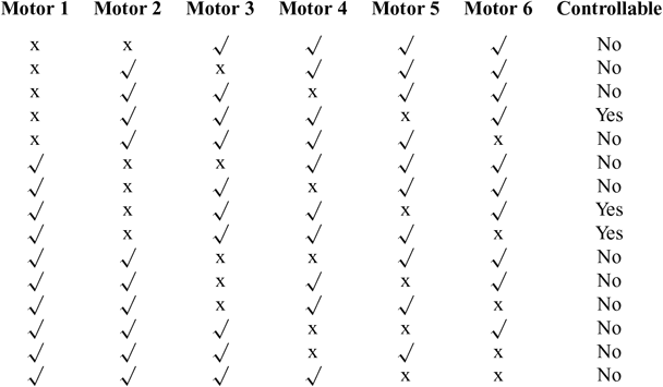
that can be solved only for α₇ + α₁₀ < 0; thus, the condition is violated and the system is not controllable. Same calculations are conducted for the other motor failure cases leading to the controllability tables (Tables 1 and 2).

Table 1

Controllability of the hexarotor UAV after one actuator failure

Table 2

Controllability of the hexarotor UAV after two actuators failures

3.3 Fault-tolerant control allocation problem

Control allocation is an actuator redundancy management technique in over-actuated systems. It arises when the system to be controlled has more physical actuators than control objectives.^{(Reference Johansen and Fossen23)} Its design is often divided into several levels (Fig. 3). First, a high-level motion control algorithm is designed to compute a vector of virtual inputs to the system. Second, a control allocation algorithm is designed in order to map the vector of commanded virtual input forces and moments into individual effector forces or moments. Third, there may be a separate low-level controller for each effector that controls its actuators in order to achieve its desired force and moment.

Figure 3.

System structure including control allocation.

For a multirotor UAV, four main control objectives must be met (the control of the roll, pitch, yaw and thrust) using the motors/propellers available. In case of one or more actuators failures, the remaining ones can be reconfigured by the control allocation system without having to change the motion controller structure and tuning. Over-actuated control allocation problems are usually formulated as optimisation problems that are hard to solve in real-time systems with limiting processing capacity.

3.4 Fuzzy logic-based control allocation

Fuzzy logic provides a means of converting a linguistic control strategy based on expert knowledge into an automatic control strategy.^{(Reference Lee24)} The fuzzy logic-based control allocation is a set of linguistic allocation rules related by the dual concepts of fuzzy implication and the compositional rule of inference. It comprises four components: the fuzzification interface, the knowledge base, the decision-making logic, and the defuzzification interface. The fuzzification interface involves the following functions: measures the states of each motor using a fault diagnosis scheme (6 inputs), then converts these input data into the suitable linguistic values T(motor state) = {faulty, normal}. The two terms in T(motor state) are characterised by a fuzzy set in a universe of discourse U = {0,1}. The knowledge base and the decision-making logic provide the set of linguistic description rules that are based on expert knowledge in the form of: IF (S₁ state = a&S₂ state = b&S₃ state = c & S₄ state = d & S₅ state = e&S₆ state = f) THEN (G₁ = A&G₂ =B&G₃ = C&G₄ = D&G₅ = E&G₆ = F) with S_i and G_i are, respectively, the state and the multiplexing gain of the i^th motor, {a, b, c, d, e, f} ∊ {faulty, normal} and {A, B, C, D, E, F} ∊ {verylow, low, lowplus, medium, bithigh, sohigh}. Finally, the defuzzifiation interface performs a scale mapping that converts the output variables into their corresponding universes of discourse. For example, we might interpret “verylow” for a multiplexing gain of “0” and “sohigh” for a multiplexing gain of “1.95”.

The control allocation problem is formulated as below (Fig. 4):

$$u(t) = \alpha (t){u_n}(t)$$ (23)

Figure 4.

Fuzzy Logic based Control Allocation.

with α(t) is the vector of allocation gains and u_n(t) the nominal control inputs. The proposed fuzzy logic fault-tolerant controller is of Sugeno-type due to the fact that it admits by experience a lower number of required rules. This control allocation has six inputs identifying the state of each motor and six outputs designating the multiplexing gains. Finally, a bacterial foraging algorithm is used to optimise the fuzzy logic outputs.

3.5 Bacterial Foraging Algorithm (BFA)

BFA is a bio-inspired non-gradient optimisation technique that has been applied in many control applications.^{(Reference Das, Biswas, Dasgupta and Abraham18)} It mimics nature and checkmates the impending problems of local optimum associated with classical procedures. Its objective is to minimise a cost function J(θ), θ ∈ R ^p. Basically, the BFA consists of four basic elements known as chemotaxis, swarming, reproduction and elimination-dispersal. A number of parameters that control the chemotactic behaviour are the number of bacteria (S), maximum number of chemotactic loop (N_c), maximum number of reproduction (N _re ), maximum number of elimination and dispersal events (N), dimension of the search space (p), probability for the elimination-dispersal event (P _ed ), swim length (N_s), counter for swim length (m) and chemotactic step sizes C(i), i = 1, 2, …, S.

Let P(j, k, l) = {θ ⁱ( j, k, l) |i = 1, 2, …, S } represent the position of each member in the population of the S bacteria at the j^th chemotactic step, k^th reproduction step and l^th elimination-dispersal event. Here, let J(i, j, k, l) denote the cost at the location of the i^th bacterium θⁱ. The four prime steps in the BFA are discussed below:

• • Chemotaxis: This process simulates the movement of an E. coli cell through swimming and tumbling and may be represented by:

  $${\theta ^i}({\kern 1pt} j + 1,k,l) = {\theta ^i}({\kern 1pt} j,k,l) + C(i){{\Delta (i)} \over {\sqrt {{\Delta ^T}(i)\Delta (i)} }}$$ (24)

  where Δ indicates a vector in the random direction whose elements lie in [−1, 1].

• • Swarming: This group behaviour is seen when bacteria propagate collectively as concentric patterns of swarms. The cell-to-cell signalling in an E. coli swarm may be represented by the following function:

  $$\matrix{ {{J_{cc}}(\theta ,P({\kern 1pt} j,k,l)) = \sum\limits_{i = 1}^S {J_{cc}}(\theta ,{\theta ^i}({\kern 1pt} j,k,l))} \hfill \cr { = \sum\nolimits_{i = 1}^S {[ - {d_{{\rm{a}}ttractant}}exp( - {w_{{\rm{a}}ttractant}}\sum\limits_{m = 1}^p {{({\theta _m} - \theta _m^i)}^2})]} } \hfill \cr { + \sum\nolimits_{i = 1}^S {[{h_{{\rm{r}}epellant}}exp( - {w_{{\rm{a}}ttractant}}\sum\limits_{m = 1}^p {{({\theta _m} - \theta _m^i)}^2})]} } \hfill \cr } $$ (25)

  where J_cc(θ, P( j, k, l)) is the objective function value to be added to the actual objective function (to be minimised) to present a time varying objective function, S is the total number of bacteria, p is the number of variables to be optimised, which are present in each bacterium, and θ = [θ ₁ θ ₂ … θ_p]^T is a point in the p-dimensional search domain. d _attractant, w _attractant, h _repellant and w _attractant are different coefficients that should be chosen properly.

• • Reproduction: The fitness value for i^th bacterium after travelling N_c chemotactic steps can be evaluated by the following equation:

  $$J_{{\rm{h}}ealth}^i = \sum\limits_{j = 1}^{{N_c} + 1} {J^i}({\kern 1pt} j,k,l)$$ (26)

  Here Jⁱ_health represents the health of i^th bacterium. The least healthy bacteria constituting half of the bacterial population are eventually eliminated while each of the healthier bacteria split into two, which are then placed in the same location. Hence, ultimately the population remains constant.

• • Elimination and Dispersal. The BFA algorithm makes some bacteria to get eliminated and dispersed with probability P _ed after N _re number of reproductive events to ensure that the bacteria do not get trapped into a local optimum instead of the global optima.

The objective of the gains tuning in our application is to recover the hexarotor UAV while following the desired trajectory. For this reason, the performance index of the system is chosen as the minimum mean squared error (MMSE) of system response to minimise the error between the desired and measured states. The MMSE is calculated for each decision variable X in the system x, y, z, ϕ, ψ and θ as follows:

$$MMSE = {\rm{m}}in[{1 \over N}\sum\limits_{i = 1}^N {({X_{{\rm{i}}d}} - {X_i})^2}]$$ (27)

X _id is the reference value of the corresponding variable X_i. The objective function is chosen as the summation of the MMSE of each variable. Hence, minimising this objective function will result in finding the optimum fuzzy logic control allocation gains with the minimum mean square error of the overall system response.

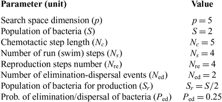
With respect to one motor failure for example, five motors work and one motor fails. Tuning shall be to the 5 multiplexing gains and, consequently, the number of variables to be optimised, which are present in each bacterium is p = 5. θ ∈ R ⁵, the vector of output scaling gains, θ =[θ ₁ θ ₂ … θ_p]^T is a point in the p-dimensional search domain. The starting number of bacteria (search agents) in the population or simply the initial solution points, which will change iteratively to lower MMSE, is chosen as S = 2. This parameter is recommended to be an even number and not so large to avoid complexity computations. The maximum number of chemotactic steps per bacteria lifetime was set to N_c = 5 after trials and observations. The starting value was 2, but there was a need to increase it to avoid being trapped at local minimum as was being observed without causing so much computational complexity. The chemotactic step sizes for each bacterium were set after multiple trials as C = [0.00001; 0.00001], since increasing this step would lead to missing the minimum and decreasing it would cause oscillations around the minimum with very slow convergence. The starting vector was C = [0.01, 0.01]). The other parameters are fixed at their default values and shown in Table 3.

Table 3

Selected parameters for BFA optimisation

4.1 Matlab simulations

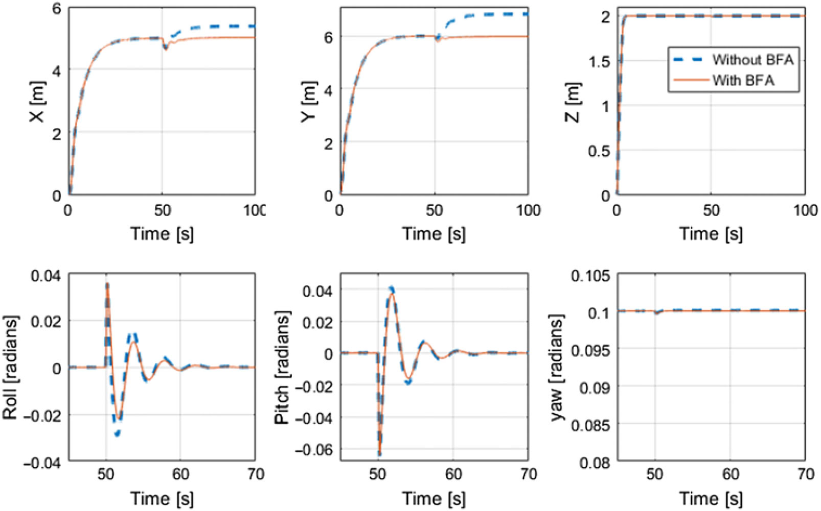
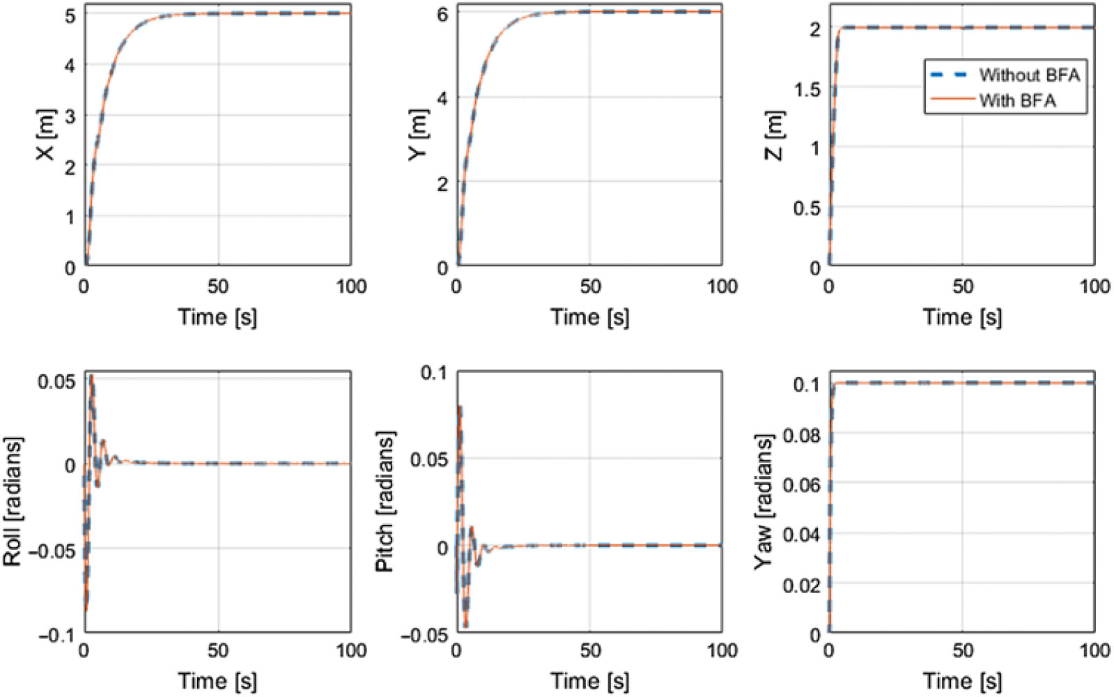
The scope of this section is to emphasise the performance of the fault tolerant control allocator by simulation. The nonlinear model of the hexarotor based on Equation (1), is implemented in Simulink. The actuators failures are simulated. The original and tuned fault-tolerant controllers are tested for the different faulty situations. In a first scenario, a failure is injected on motor 1, and in a second scenario, two failures are injected on motors 2 and 5. Each time, the failure is activated at t = 40 s, and each fault-tolerant controller is put into action after a delay of 0.2 s in order to test the response time of the controller and its possible realistic operation. The results are examined in Figs. 5 and 6, where the blue line corresponds to the case of fault-tolerant controller with no tuning, while the red one corresponds to the case of the tuned controller. It can be shown that the original fuzzy logic-based fault-tolerant controller generally provides a satisfactory control allocation technique following the different fault configurations. However, the tuned controller is a bit modified from the original controller using the BFA optimisation technique to ensure an optimal fuzzy control allocation at all times. The remarkable improvement appears in the behaviour of the tuned controller following the motor 1 fault, in comparison with the behaviour of the original fuzzy fault-tolerant controller.

Figure 5.

Simulation results of the hexarotor in case of one motor failure (motor 1).

Figure 6.

Simulation results of the hexarotor in case of two motor failures (motors 2 and 5).

4.2 Experimental validation

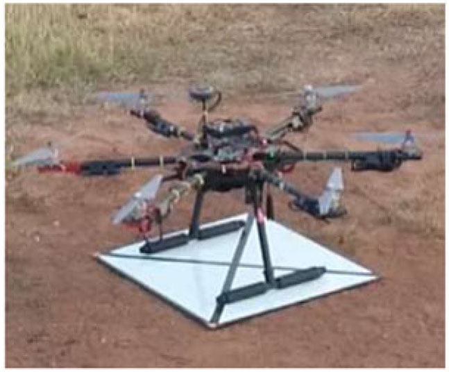
The testbed is a Tarothexacopter as seen in Fig. 7. It is a PPNNPN hexarotor, which uses DJI 2312 960KV motors driven with DJI 40 Amp ESC. For flight tests, the architecture runs on a Pixhawk flight controller, an open source robust autopilot controller based on a 32-bit ARM CPU connected to an IMU and Barometric Altimeter and equipped with needed digital communication peripherals. For position control, a low-cost Ublox M8N GPS is connected to the Pixhawk through a serial port and managed by the mounted CPU. For the flight test, the parameters in Table 3 have been used ^{Footnote 1}.

Figure 7.

The experimental hexarotor UAV.

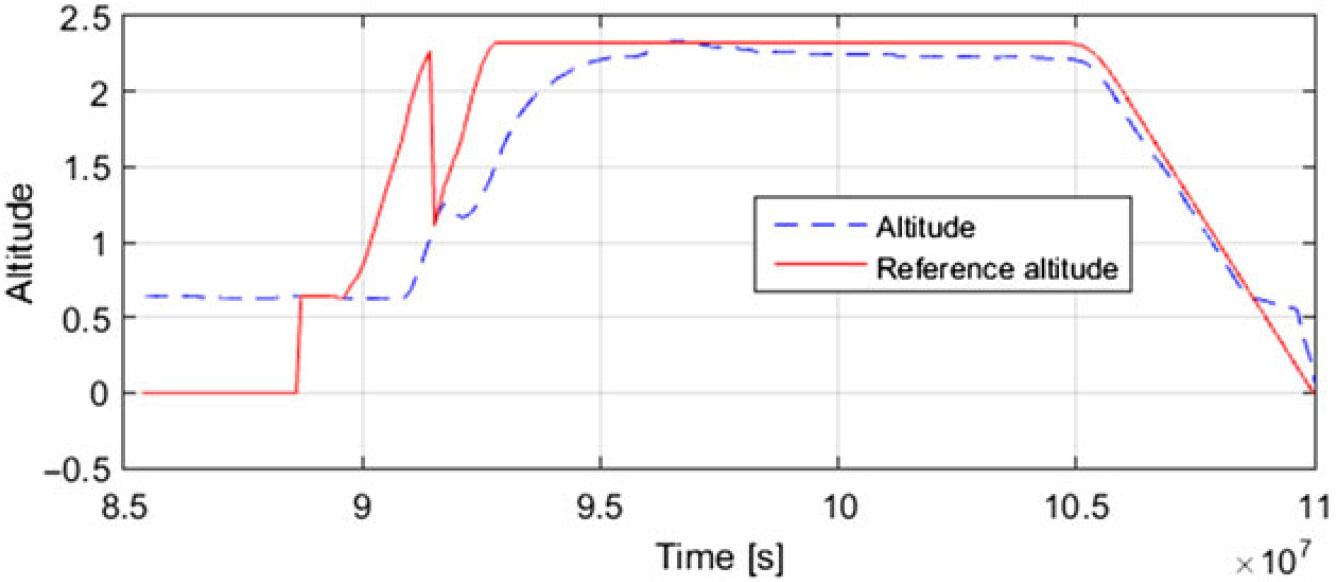
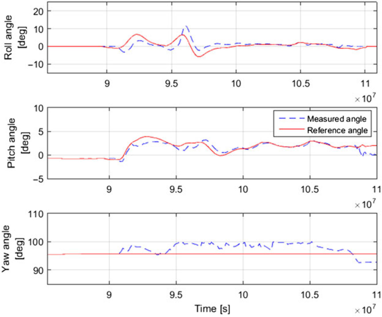
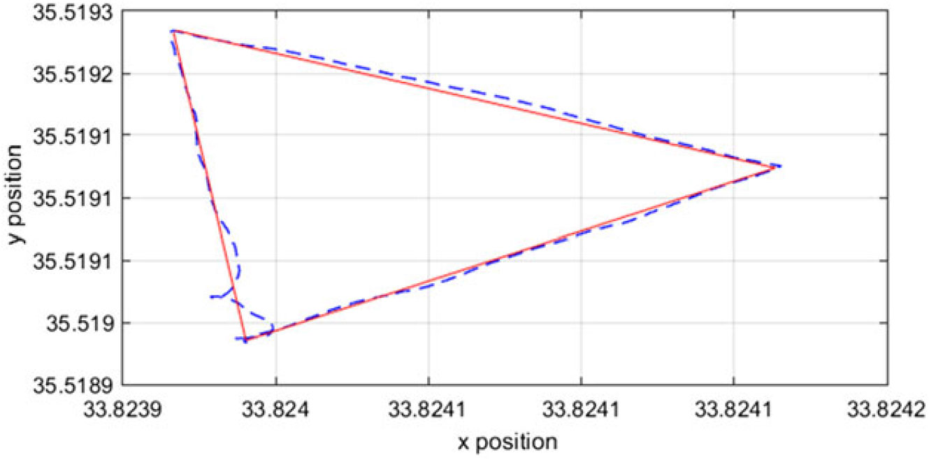
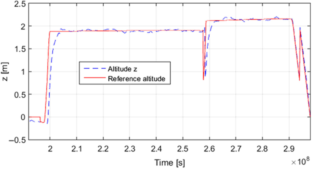
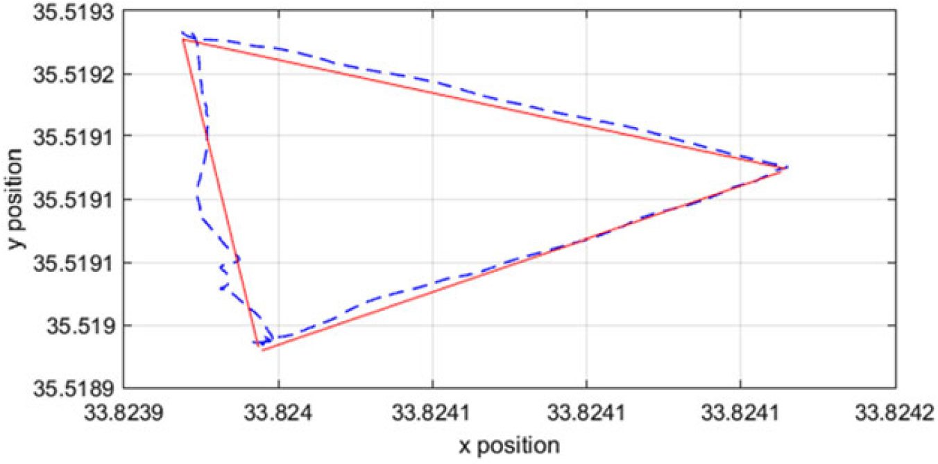
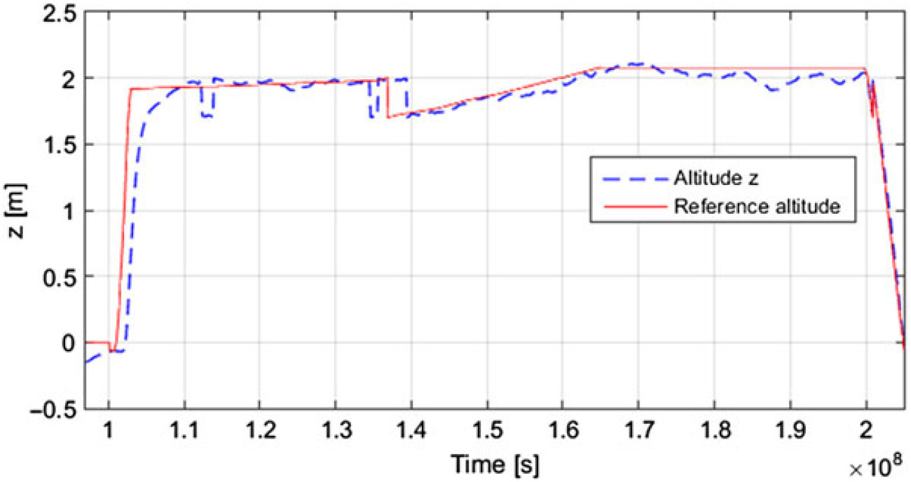
In order to reproduce the conditions of a real actuator failure, the motor is turned off online from the RC transmitter. Figures 8–11 show the flight test results during hovering and when following a trajectory after two motors failures. In each case, the control allocator is reconfigured after 0.2 s from the failure injection. It can be seen that during hovering and as time increases, the roll, pitch and yaw angles and the altitude are able to follow their varying reference signals, respectively. In the second scenario, the hexarotor is able to complete a suitable triangular trajectory, despite of the activated two motor failures, by taking advantage of the generated fuzzy logic control gains. Generally, the altitude is maintained constant within a small level of error tolerance. Figures 12 and 13 show the flight test results after one motor failure.

Figure 8.

Experimental altitude results in case of two motor faults during hovering.

Figure 9.

Experimental attitude results in case of two motor faults during hovering.

Figure 10.

Trajectory in case of two motor failures.

Figure 11.

Altitude during trajectory in case of two motor failures.

Figure 12.

Trajectory in case of one motor failure.

Figure 13.

Altitude during trajectory in case of one motor failure.