
I. INTRODUCTION
Cellular materials are porous materials with lower bulk density than that of their constitutive materials. These materials tend to be heavily interconnected with a high surface area (SA) and low density. They are useful in a wide variety of applications, Reference Evans, Hutchinson, Fleck, Ashby and Wadley1 such as sandwich structure cores, Reference Chiras, Mumm, Evans, Wicks, Hutchinson, Dharmasena, Wadley and Fichter2,Reference Wicks and Hutchinson3 energy absorption, Reference Schaedler, Ro, Sorensen, Eckel, Yang, Carter and Jacobsen4,Reference Evans, He, Deshpande, Hutchinson, Jacobsen and Carter5 thermal management, Reference Lu, Stone and Ashby6–Reference Roper, Schubert, Maloney, Page, Ro, Yang and Jacobsen8 bio scaffolds, Reference Jones, Lin, Yue, Lee, Hanna, Smith and Newport9 and acoustics. Reference Lu, Hess and Ashby10
The performance of cellular materials is dominated by three major factors: material, architecture, and relative density. Reference Ashby11 To properly design a cellular material for a given application, each of these three factors must be determined. The base material choice is important since the properties of the constituent solid are extended to the individual members that make up the porous material. The architecture dictates the behavior of the porous material as a whole and includes open or closed cell pore types and stochastic or periodic cell structures. Reference Wadley12 Finally, the relative density is of paramount importance because many properties scale according to a power-law relationship with relative density, depending on the architecture. Reference Finnegan, Kooistra, Wadley and Deshpande13
Many types of architectures exist for cellular materials. Stochastic foams have been in production for decades and the physical properties of many of these porous materials, both open cell and closed cell, have been extensively investigated and characterized. Reference Gibson and Ashby14–Reference Gibson, Ashby and Harley16 While stochastic foams excel in energy absorption due to their near-constant plateau stress, Reference Gibson and Ashby15 the random nature of the foam results in a bending-dominated structure that has decreased stiffness. Reference Deshpande, Ashby and Fleck17 Furthermore, while the bulk material properties of these foams can be tailored for a specific application, the random nature of the structure and lack of the unit cell make it difficult to tailor on the microscale.
Architected cellular materials, on the other hand, are well ordered and have repeating unit cells. Their mechanical response can be tailored to be stretch dominated, resulting in high stiffness that is typically unattainable by stochastic foams. Reference Deshpande, Ashby and Fleck17–Reference Zheng, Lee, Weisgraber, Shusteff, DeOtte, Duoss, Kuntz, Biener, Ge, Jackson, Kucheyev, Fang and Spadaccini19 Unlike stochastic foams, periodic lattice cellular materials have a repeating unit cell pattern, thus it is possible to accurately characterize the geometric properties of these materials such as volume fraction and surface-area-to-volume ratio (i.e., compactness) from unit cell dimensions and angles. Many types of architected cellular materials exist. Geometries of particular interest include woven textiles, honeycombs, corrugated sheets, prismatic cells, and lattice porous materials. Reference Lu, Valdevit and Evans20,Reference Wadley, Fleck and Evans21 Lattice porous materials such as pyramidal, Reference Queheillalt and Wadley22 tetrahedral, Reference Kooistra, Deshpande and Wadley23 and 3-D Kagomé Reference Wang, Evans, Dharmasena and Wadley24 are of particular interest, and their mechanical properties have been analyzed.
New, scalable methods of fabricating solid and hollow square-pyramidal and tetrahedral architected lattice materials have been recently developed. Reference Jacobsen, Barvosa-Carter and Nutt18,Reference Jacobsen, Barvosa-Carter and Nutt25–Reference Schaedler, Jacobsen, Torrents, Sorensen, Lian, Greer, Valdevit and Carter27 Open-cellular, lattice porous materials are formed from intersecting, self-propagating photopolymer waveguides. Reference Jacobsen, Barvosa-Carter and Nutt28 In the simplest method of fabrication, the final product is comprised of circular cylinders that intersect at nodes. The number of cylinders depends on the architecture: pyramidal and tetrahedral porous materials are comprised of four and three intersecting cylinders, respectively. A variety of architectures can be fabricated depending on the number of waveguides, the cross-sectional geometry of the waveguides, and the pattern of waveguides used. The mechanical, fluidic, and heat transfer properties of some of these lattice porous materials have been experimentally characterized. Reference Maloney, Roper, Jacobsen, Carter, Valdevit and Schaedler26,Reference Fink, Kolodziejska, Jacobsen and Roper29,Reference Roper, Fink, Lee, Kolodziejska and Jacobsen30 Combining these properties enables the design of multifunctional porous materials that are highly desirable in systems that have stringent weight or space requirements.
The design of architected cellular materials can be tailored to maximize the benefit in any given application through optimization. Reference Wicks and Hutchinson31,Reference Valdevit, Jacobsen, Greer and Carter32 The geometric properties of the porous material must be properly characterized to perform optimization. Several geometric properties are particularly important for different physical processes. The solid volume fraction is important for mechanical strength and acoustics. Porosity is important for fluid flow. Compactness is important for the diffusion-based processes such as heat and mass transfer. While these properties can be obtained numerically, analytical equations for these geometric properties are desirable because they enable computationally efficient multiobjective optimization. Furthermore, analytical equations simplify the initial design by removing the need to perform numerical computation to obtain an accurate result.
Previous work exploring architected lattice cellular materials has focused on modeling physical properties. Reference Jacobsen, Barvosa-Carter and Nutt18,Reference Jacobsen, Barvosa-Carter and Nutt33,Reference Wadley34 Models for the physical properties of porous materials use geometric models as inputs, thus the accuracy of the physical models is dependent on the accuracy of the geometric models. However, typical models for the geometric properties of lattice porous materials make simplifying approximations that introduce errors, especially at high solid volume fractions. For instance, approximations are typically made that define the structure such that the volume of intersection is ignored. Reference Evans, He, Deshpande, Hutchinson, Jacobsen and Carter5,Reference Maloney, Fink, Schaedler, Kolodziejska, Jacobsen and Roper7,Reference Jacobsen, Barvosa-Carter and Nutt18,Reference Jacobsen, Barvosa-Carter and Nutt25,Reference Deshpande, Fleck and Ashby35–Reference Valdevit, Godfrey, Schaedler, Jacobsen and Carter37 Efforts have been made to account for the volume of intersection, Reference Hammetter, Rinaldi and Zok38 but accurate analytical equations for compactness do not currently exist. Ignoring the volume of intersection is a reasonable approximation for materials comprised of long, slender struts but is inaccurate for higher-density porous materials. This error then propagates through the existing models for the structural and thermal properties of lattice porous materials. Reference Jacobsen, Barvosa-Carter and Nutt18,Reference Jacobsen, Barvosa-Carter and Nutt33,Reference Wadley34,Reference Roper39 For intersecting cylinders, a common feature in lattice porous materials, the intersecting volume is known as a Steinmetz solid. For two cylinders intersecting at a right angle, a Steinmetz solid consists of two base-to-base square pyramids which taper nonlinearly. The solution for the intersecting volume has been extended to multiple cylinders, Reference Moreton40,Reference Angell and Moore41 but these solutions are found only for very specific orientations of solid cylinders.
This work develops closed-form analytical equations for the solid volume fraction and compactness of lattice porous materials with struts having circular cross sections. Architectures considered include rectangular prism and hexagonal prism unit cells as well as solid and hollow struts. The application of these equations over a wide range of parameters is investigated and a comparison to prior approximations is presented.
II. ANALYTICAL EQUATIONS
Several variations of intersecting cylinders are of interest for lattice porous materials. Derivations for the solid volume fraction
 $\left( {\bar{\rho }} \right)$
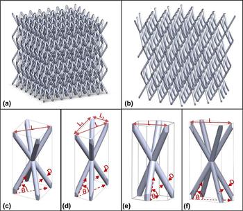
and compactness (β) for pyramidal and tetrahedral lattices are presented. Two variations of pyramidal lattices are derived: square prism unit cells with circular cylinders [Fig. 1(c)] and rectangular prism unit cells with circular cylinders [Fig. 1(d)]. One variation is derived for hexagonal prism unit cells with circular cylinders [Fig. 1(e)]. All variations are modeled for both solid cylinders as well as hollow cylinders [Fig. 1(f)].
Schematics of (a) one pyramidal lattice cellular material; (b) one tetrahedral lattice cellular material; and unit cells for various pyramidal and tetrahedral lattice cellular materials: (c) square prism with circular cylinders; (d) rectangular prism with circular cylinders; (e) hexagonal prism with circular cylinders; and (f) rectangular prism with hollow circular cylinders.

A. Square prism unit cell
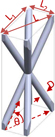
The square prism unit cell of the pyramidal lattice consists of four cylinders that each connect opposite corners of an imaginary square prism [Fig. 1(c)]. The cylinders intersect at the center of the prism and are truncated where they extend past the boundary of the square prism. The diameter (D) and inclination angle (θ) are the same for each cylinder. L is defined as
 $\sqrt 2$
times the unit cell base length to maintain consistency with earlier definitions in the literature.
Reference Jacobsen, Kolodziejska, Doty, Fink, Zhou, Roper and Carter42
It is sufficient to consider a single unit cell to determine the solid volume fraction and compactness of the bulk geometry. The volume of the square prism is given by the following:
 $$V = {{{L^3}\tan \theta } \over 2}\quad .$$
A simple approximation to the solid volume fraction can be made by dividing the volume of four cylinders by the volume of the square prism which simplifies to the following:
 $${\bar{\rho }_{{\rm{approx}}}} = {{2\pi {D^2}} \over {{L^2}\sin \theta }}\quad .$$
Equivalent forms of this equation can be found, e.g., in Ref. Reference Deshpande and Fleck36 Eq. (A.12) and Ref. Reference Jacobsen, Barvosa-Carter and Nutt18 Eq. (1). Similar forms for tetrahedral lattices can be found, e.g., in Ref. Reference Deshpande and Fleck36 Eq. (A.1) and Ref. Reference Jacobsen, Barvosa-Carter and Nutt25 Eq. (2). This approximation quadruple, triple, and double counts the various regions of the intersection volume at the center of the square prism and does not account for the truncated ends of the cylinders. When the cylinders are slender (i.e., L/D ≫ 1) and the inclination angle is not close to 0 or π/2, this is a reasonable approximation.
Developing models for the solid volume fraction that do not depend upon the choice of the unit cell parameters requires a more detailed model development. Such exact formulas will be applicable to a wide range of unit cell parameters and, in particular, will be accurate for low aspect ratio (L/D) cylinders.
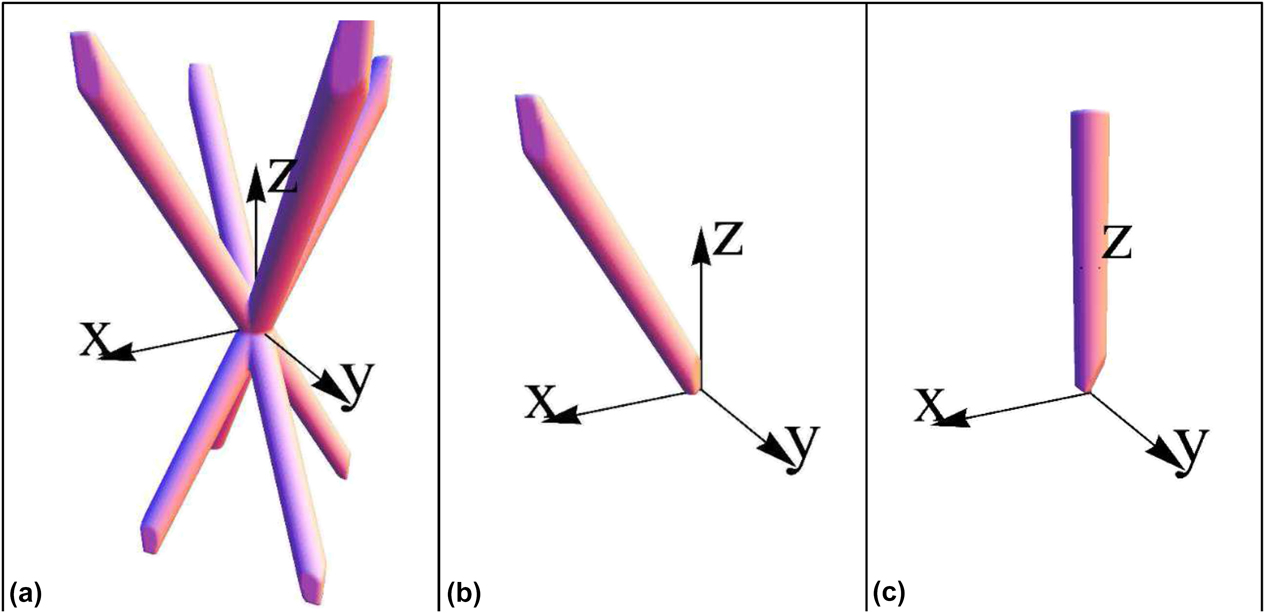
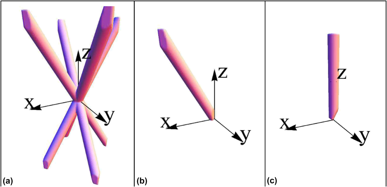
Figure 2 shows the generic simplification process used to develop the model. The symmetry can be utilized to simplify the geometry of a single unit cell [Fig. 2(a)]. A single strut [Fig. 2(b)] is repeated eight times per unit cell, while a half strut [Fig. 2(c)] is repeated sixteen times per unit cell. The half strut is used as the base geometry from which the overall volume can be calculated.
The generic simplification process for model development (a) full unit cell; (b) single strut; and (c) half strut rotated to align with the z-axis.
A semi-infinite single strut aligned with the x–z plane can be represented by the following inequalities:
 $$\matrix{ {{{\left( {x\cos \left( {{\pi \over 2} - \theta } \right) - z\sin \left( {{\pi \over 2} - \theta } \right)} \right)}^2} + {y^2} \lt {{\left( {{D \over 2}} \right)}^2}\quad ,} \cr {y \lt x\quad ,} \cr {y > - x\quad ,} \cr {z > 0\quad ,} \cr}$$
The inequalities above define a semi-infinite single strut that extends beyond the unit cell boundaries. The strut is rotated in the x–z plane by the complement of the inclination angle (π/2 − θ), so the cylinder axis aligns with the z-axis [Fig. 2(c)]. This rotation shifts the complexity from the integrand to the limits of integration, thus making the integral solution easier. Applying this rotation to the bounding planes results in the following inequalities:
 $$\matrix{ {{x^2} + {y^2} \lt {{{D^2}} / {4\quad ,}}} \cr {y \lt x\sin \theta + z\cos \theta \quad ,} \cr {y > - x\sin \theta - z\cos \theta \quad ,} \cr {z\sin \theta - x\cos \theta > 0\quad .} \cr}$$
The three planes provide bounds of integration for a volume integral of a bounded cylinder. Transforming the equations into cylindrical coordinates (r, γ, z) yields the following inequalities:
 $$\matrix{ {r \lt {D / {2\quad ,}}} \cr {{\rm{plane}}\;1{\rm{:}}\;r\sin \gamma \lt r\cos \gamma \sin \theta + z\cos \theta \quad ,} \cr {{\rm{plane}}\;2{\rm{:}}\;r\sin \gamma > - r\cos \gamma \sin \theta - z\cos \theta \quad ,} \cr {{\rm{plane}}\;3{\rm{:}}\;z\sin \theta - r\cos \gamma \cos \theta > 0\quad .} \cr}$$
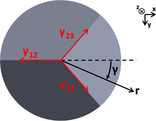
All three bounding planes intersect at the origin, but each pair of planes also intersects along a line. Each line yields a bound of integration for the volume integral. After solving for all three intersections, it can be shown that the intersections correspond with the following equations:
 $$\matrix{ {{\gamma _{13}} = {{\tan }^{ - 1}}\left( {\csc \theta } \right)\quad ,} \cr {{\gamma _{23}} = - {{\tan }^{ - 1}}\left( {\csc \theta } \right)\quad ,} \cr {{\gamma _{12}} = \pi \quad .} \cr}$$
Here γ ij corresponds to the projected angle in the r–γ plane that describes the intersection of planes i and j, as shown in Fig. 3.
Cross-sectional view of the intersection of the cut planes [strut in Fig. 2(c) viewed from origin looking in the +z direction].
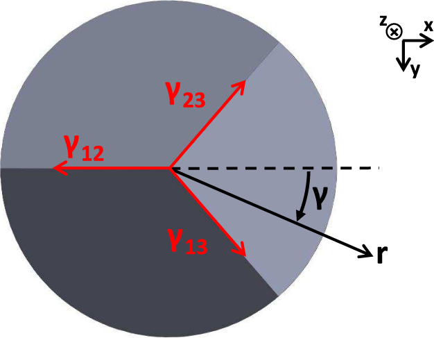
These angles describe the bounds of integration for the γ coordinate. Since the radius of the strut is constant, the bounds of integration for the r coordinate are from 0 → D/2. Finally, the bounds of integration for the z coordinate must be found. Since the bounding planes differ for different ranges of γ, the volume integral is piecewise. The lower bound of integration of each piecewise integral is given by the equation of the bounding plane in each range of γ. The upper bound of integration is chosen such that symmetry can be applied, resulting in half the length of the strut. In terms of the known lattice parameters, this half-strut length is:
 $$c = {L \over {4\cos \theta }}\quad .$$
These bounds are used in a piecewise volume integral to solve for the volume of the half strut:
 $$V = \int_{{\gamma _{23}}}^{{\gamma _{13}}} {\int_0^{D{\rm{/}}2} {\int_{{z_3}}^c {r{\rm{d}}z{\rm{d}}r{\rm{d}}\gamma } } } + \int_{{\gamma _{13}}}^{{\gamma _{12}}} {\int_0^{D{\rm{/}}2} {\int_{{z_1}}^c {r{\rm{d}}z{\rm{d}}r{\rm{d}}\gamma } } } + \int_{{-\gamma _{ 12}}}^{{\gamma _{23}}} {\int_0^{D{\rm{/}}2} {\int_{{z_2}}^c {r{\rm{d}}z{\rm{d}}r{\rm{d}}\gamma } } \quad ,}$$
Here z i is the equation of the bounding plane from Eq. (5) that is between the two angles of integration when solved for z.
This integral is the generic form used for the following equation derivations with circular cylinders. In the special case of the square prism unit cell comprised of circular cylinders, the half strut is symmetric about γ = 0 and γ = π, resulting in the following integral:
 $$V = 2\left( {\int_0^{{\gamma _{13}}} {\int_0^{D{\rm{/}}2} {\int_{{z_3}}^c {r{\rm{d}}z{\rm{d}}r{\rm{d}}\gamma } } } + \int_{{\gamma _{13}}}^\pi {\int_0^{D{\rm{/}}2} {\int_{{z_1}}^c {r{\rm{d}}z{\rm{d}}r{\rm{d}}\gamma } } } } \right)\quad .$$
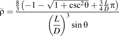
Mathematica® is used to integrate this volume integral, producing the volume of a single half strut. The solid volume fraction is calculated by multiplying this result by 16 (symmetry) and dividing by the volume of the unit cell, yielding the following equation:
 $${\bar{\rho }_{\rm{s}}} = {{{8 \over 3}\left( { - 1 - \sqrt {1 + {{\csc }^2}\theta } + {3 \over 4}{L \over D}\pi } \right)} \over {{{\left( {{L \over D}} \right)}^3}\sin \theta }}\quad .$$
For solid lattices, the porosity and external volume fraction (φo) are equivalent and are defined by the volume that is not occupied by the lattice, given by the difference between unity and the solid volume fraction.
 $${\varphi _{{\rm{s}},{\rm{o}}}} = 1 - {\bar{\rho }_{\rm{s}}}\quad .$$
Solutions for the solid volume fraction of hollow lattices are also of interest [see Fig. 1(f) for geometry].
The hollow lattice solid volume fraction is found using the same method as the solid lattice, with the only variation being the bounds of integration for the r coordinate. Given a thickness, t, the volume integral can be set up as follows:
 $$V = 2\left( {\int_0^{{\gamma _{13}}} {\int_{D{\rm{/}}2}^{D{\rm{/}}2 + t} {\int_{{z_3}}^c {r{\rm{d}}z{\rm{d}}r{\rm{d}}\gamma } } } + \int_{{\gamma _{13}}}^\pi {\int_{D{\rm{/}}2}^{D{\rm{/}}2 + t} {\int_{{z_1}}^c {r{\rm{d}}z{\rm{d}}r{\rm{d}}\gamma } } } } \right)\quad .$$
Evaluating this integral and solving for the solid volume fraction in the same fashion as the solid lattice yields the following solution for the wall volume fraction of a hollow lattice:
 $${\bar{\rho }_{{\rm{s,hollow}}}} = {{{8 \over 3}{t \over D}\left[ { - 2\left( {1 + \sqrt {1 + {{\csc }^2}\theta } } \right)\left( {3 + 6\left( {{t \over D}} \right) + 4{{\left( {{t \over D}} \right)}^2}} \right) + 3\pi {L \over D}\left( {1 + {t \over D}} \right)} \right]} \over {{{\left( {{L \over D}} \right)}^3}\sin \theta }}\quad .$$
The solid volume fraction can also be found by evaluating Eq. (10) with a diameter of D + 2t and subtracting the value obtained from evaluating the same equation with a diameter of D.
A hollow lattice consists of three distinct volumes: inside the lattice walls, the walls, and outside the lattice walls. The internal volume fraction, φi, is equivalent to the solid volume fraction for a solid lattice of equivalent geometric parameters (D, L, θ), given by Eq. (10). The external volume fraction is given by:
 $${\varphi _{{\rm{s}},{\rm{o}}}} = 1 - {\varphi _{{\rm{s}},i}} - {\bar{\rho }_{{\rm{s}},{\rm{hollow}}}}\quad .$$
Compactness (β) can be found using a similar method. Using the same rotations, cut planes, and symmetry, a double integral for the surface area (SA) can be posed in the following form:
 $${\rm{SA}} = \int_{{\gamma _{23}}}^{{\gamma _{13}}} {\int_{{z_3}}^c {{\rm{d}}z{\rm{d}}s} } + \int_{{\gamma _{13}}}^{{\gamma _{12}}} {\int_{{z_1}}^c {{\rm{d}}z{\rm{d}}s} } + \int_{{- \gamma _{ 12}}}^{{\gamma _{23}}} {\int_{{z_2}}^c {{\rm{d}}z{\rm{d}}s} } \quad ,$$
where ds is the line element around the circumference of the cylinder.
In the case of circular cylinders, the line integral ds can be represented by ds = rdγ. Setting up the integral with the same bounds of integration for z and γ as in the volume integral yields the following:
 $${\rm{SA}} = 2\left( {\int_0^{{\gamma _{13}}} {\int_{{z_3}}^c {r{\rm{d}}z{\rm{d}}\gamma } } + \int_{{\gamma _{13}}}^\pi {\int_{{z_1}}^c {r{\rm{d}}z{\rm{d}}\gamma } } } \right)\quad .$$
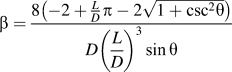
Solving this integral, multiplying by 16 (symmetry), and dividing by the unit cell volume yields the following closed-form solution for the compactness of a solid lattice:
 $${\beta _{\rm{s}}} = {{8\left( { - 2 + {L \over D}\pi - 2\sqrt {1 + {{\csc }^2}\theta } } \right)} \over {D{{\left( {{L \over D}} \right)}^3}\sin \theta }}\quad .$$
It should be noted that the compactness given above has units of 1/length.
In the case of hollow lattices, Eq. (17) or Table III can be used to find the inner compactness (βi) of the lattice. The outer compactness (βo) can be found by adding twice the wall thickness to the diameter and reevaluating the equation. Note that this substitution should be made in both the D and L/D terms.
B. Nonsquare rectangular prism unit cell
The equations derived so far are limited to lattices with a square pattern of nodes. A more generic geometry is found when the top and bottom square faces of the unit cell are replaced by nonsquare rectangular faces [Fig. 1(d)]. The diameter (D) and inclination angle (θ) remain unchanged. The longer and shorter sides of the rectangular faces are designated L 1 and L 2, respectively. The ratio of the side lengths, L 1/L 2, is defined as α. In order for the nonsquare rectangular prism and square prism geometries to be equivalent in the limit of L 1 → L 2, the following relationship is defined for the lattice spacing (L):
 $$L = \sqrt {L_1^2 + L_2^2} \quad .$$
The volume of the nonsquare rectangular prism unit cell is given by the following equation:
 $$V = {L_1}{L_2}L\tan \theta \quad .$$
The same derivation steps as used in the square prism unit cell can be used in the nonsquare rectangular prism unit cell. The derivation methods begin to diverge at the definition of the bounding planes since the nonsquare nature of the unit cell must be considered. The nonsquare nature of the unit cell also causes the piecewise integration to no longer be symmetric about any line, and as a result, all three bounding planes must be used in Eqs. (8) and (15) to solve for the volume and surface area.
The symmetry conditions, bounding planes, integration angles, and half-strut lengths for the nonsquare rectangular prism unit cell are given in Table I. Once all of these parameters are determined for a given geometry, the equation derivation procedures for volume fractions and the compactness of solid and hollow geometries given for the square prism unit cell are applicable. These equations are given in Tables II and III.
Integration parameters for each structure type.


Compactness equations.

C. Hexagonal prism unit cell
The hexagonal prism unit cell lattice is constructed in a similar fashion to the square prism unit cell but with the base unit cell shape as a hexagonal prism [Fig. 1(e)]. The struts intersect at the center of the hexagonal prism. The nodes are positioned at the vertices of the top and bottom faces of the hexagonal prism such that each node is equidistant from the center of the face. Diameter (D) and inclination angle (θ) are defined in the same way as the square prism unit cell. The distance L is instead defined as the smallest distance between the nodes on the face of the hexagonal prism.
Similar steps as those used in the derivation of the square prism unit cell are used to derive the equations for the solid volume fraction and compactness of the hexagonal prism unit cell. Since the unit cells differ so do the symmetry and bounding planes.
The volume of the hexagonal unit cell is given by V = L 3 tan θ.
Symmetry is applied such that the hexagonal unit cell is divided into three equal volumes, with exactly one strut in each section. The strut is divided in half in the same manner as the square prism unit cell. Since the rotated cylindrical strut is symmetric about γ = 0 and γ = π, the piecewise triple integral can be integrated over half of the cylinder. The triple integral in Eq. (9) can then be used with the appropriate bounds of integration to calculate the volume of the strut.
The symmetry conditions, bounding planes, integration angles, and half-strut lengths for the hexagonal prism unit cell are given in Table I. Once all of these parameters are determined for a given geometry, the solution procedures for volume fractions and compactness of the solid and hollow geometries given for the square prism unit cell are applicable. These solutions are given in Tables II and III.
III. RESULTS
The equations for solid volume fraction and compactness are valid for porous materials comprised of circular cylinders such that the nodes do not touch one another. For square prism structures, this corresponds to a lower limit of L/D > 2. The range of interest for lattice porous materials is approximately 4 < L/D < 20. L/D < 4 produces extremely dense structures, which are more similar to a solid with sparsely spaced voids than an open lattice. L/D > 20 produces structures with extremely slender struts, which are unlikely to be self-supporting under gravitational loads.
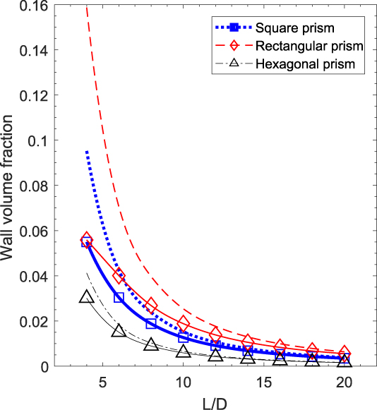
Figure 4 shows the solid volume fraction for each geometry across a range of 4 ≤ L/D ≤ 20. Due to the large number of possible variations, a select number of variations are chosen that represent the practical limits of each type of structure. For the nonsquare rectangular prism unit cell, L 1/L 2 = 3 is chosen. θ = π/3 and t/D = 0.05 is selected for each geometry. The nonintersecting cylinders approximation given in Eq. (2) is plotted as a reference. Numerical results obtained from SolidWorks® are shown as points and are used as reference for the analytically derived solution.
Solid volume fraction for hollow structures: (solid lines) new analytical equations—this work, Eq. (13) for square prisms and applying Eq. (14) at D and D + 2t for φs,i and φs,o, respectively, to Table II for rectangular and hexagonal prisms; (open symbols) numerical model comparison; and (dashed lines) previous approximate equations which include overlapping volumes and can be found, e.g., in Ref. Reference Evans, He, Deshpande, Hutchinson, Jacobsen and Carter5 Eq. (12) and Ref. Reference Valdevit, Godfrey, Schaedler, Jacobsen and Carter37 Eq. (2).
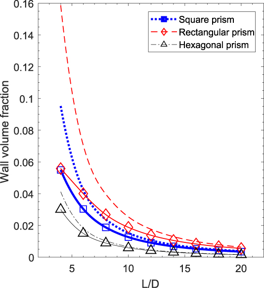
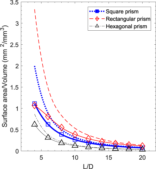
Figure 5 shows the same geometries and conditions as Fig. 4 with D = 1 mm but evaluates compactness instead.
External compactness for hollow structures: (solid lines) new analytical equation—this work, Table III; (open symbols) numerical model; and (dashed lines) previous approximate equations, which can be found, e.g., as the inverse of Eq. (10) in Ref. Reference Maloney, Fink, Schaedler, Kolodziejska, Jacobsen and Roper7.
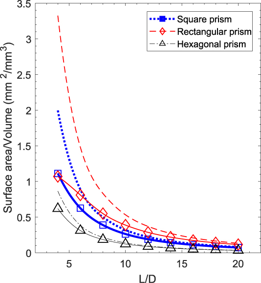
Figures 4 and 5 both show that the approximations and models converge to the same value in the limit as L/D → ∞. As L/D → 2, the solutions noticeably diverge because as the struts become less slender, the node takes up more volume relative to the struts. For these configurations, the values of the new analytically derived equations are within 0.1% of the numerical results in the entire range of 4 < L/D < 20. This is far superior to the previous approximations which have errors as large as 184% for the hollow lattice volume fraction and 211% for compactness.
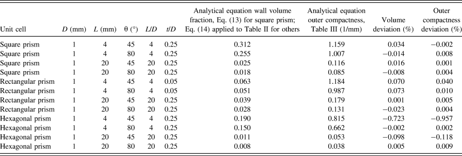
Figures 4 and 5 both show a limited set of configurations of geometric parameters for each structure type. To capture the accuracy of the solutions across a wider range of parameters, the solutions have been evaluated analytically and numerically in four combinations at the extremes of each parameter. The comparison of these results is shown in Table IV. The analytical solutions are accurate to within 0.1% for square and rectangular prism solutions. The positive and negative deviations exist due to the numerical error in evaluating the solid body models created as references in SolidWorks®. Hexagonal prism solutions start to deviate from the numerical result at very low L/D at the higher angles and higher t/D in Table IV cases because of the lack of mirror symmetry between the upper and lower half unit cells. The analytical model does not account for the lack of symmetry and in these cases results in a negative deviation since the volume evaluated in the analytical solution is slightly smaller than the actual volume numerically estimated in the solid body model. Hollow geometries have 1% deviation from the numerical result at L/D = 4 and θ = π/4 but rapidly increase the accuracy as L/D and θ are increased.
Percent deviation of analytical equations from the numerical result for twelve hollow lattice geometries.

IV. SUMMARY AND CONCLUSIONS
Closed-form analytical equations for volume fractions and compactness for architected lattice cellular materials comprising solid and hollow interpenetrating cylinders have been derived. The methodology enables the derivation of analytical solutions for volume fractions and compactness of geometries with varying numbers of cylinders and unit cell types. Comparison with numerical results shows that the solutions are accurate to 1% of volume fractions and compactness, a significant improvement over previous approximate models which had errors as large as 184% for the hollow lattice volume fraction and 211% for compactness. These analytical solutions will enable rapid optimization of physical properties based on geometric inputs, faster and more accurate design by removing the need for numerical integration or approximation, and analysis of data based on geometric parameters. They can ultimately serve as the basis from which correlations can be developed to predict the geometric properties of fabricated structures that contain imperfections and manufacturing variations to enable robust optimization of designed architected cellular materials.
NOMENCLATURE

ACKNOWLEDGMENTS
This material is based upon work supported by the U.S. Government under Contract No. W91CRB-10-C-0305. The views and conclusions contained in this document are those of the authors and should not be interpreted as representing the official policies, either expressly or implied, of the U.S. Government. The authors would like to thank Tobias Schaedler and Alan Jacobsen (HRL Laboratories, LLC) for useful discussions.