


1. Introduction
In recent years, machine learning (ML) algorithms have been increasingly applied to complex observational datasets (Sen et al. Reference Sen, Agarwal, Chakraborty and Singh2022), uncovering patterns and dependencies that are difficult to detect with traditional statistical methods. ML is widely used in astronomy for tasks ranging from galaxy classification to transient detection (Aniyan and Thorat Reference Aniyan and Thorat2017; Dax et al. Reference Dax, Green, Gair, Macke, Buonanno and Schölkopf2021) and is increasingly applied to star formation studies. For example, Marton et al. (Reference Marton, Ábrahám, Szegedi-Elek, Varga, Kun, Kóspál, Varga-Verebélyi, Hodgkin, Szabados, Beck and Kiss2019) combined Gaia DR2, WISE, and Planck data to construct an all-sky probabilistic catalogue of over one million young stellar objects (YSO) candidates, while Angarita et al. (Reference Angarita, Chaparro, Lumsden, Walsh, Avison, Asabre Frimpong and Fuller2025) used ML on millimetre spectra of massive YSO to identify spectral signatures linked to physical conditions. These studies demonstrate the ability of ML to extract meaningful information from large and complex datasets.
In this study, we explore ML methods for automated identification and classification of molecular clumps at different evolutionary stages using multi-wavelength millimetre and infrared data. For unsupervised analysis, clustering algorithms reveal natural groupings of clumps, while supervised classification uses labelled sources to classify objects with uncertain evolutionary stages.
2. Archival Datasets
We collected emission intensities of molecular lines and flux densities of the dust emission at 870
 $\mu$
m from the MALT90 dataset (Rathborne et al. Reference Rathborne, Whitaker, Jackson, Foster, Contreras, Stephens, Guzmán, Longmore, Sanhueza, Schuller, Wyrowski and Urquhart2016) using the VizieR databaseFootnote †. Infrared data at 3.6, 4.5, 8, and 24
 $\mu$
m were retrieved from the Spitzer Heritage ArchiveFootnote ‡. We also included data on class II
 $\mathrm{CH}_{3}\mathrm{OH}$
masers within 5
 $^{{\prime}{\prime}}$
of sources from the maser database (Ladeyschikov et al. Reference Ladeyschikov, Bayandina and Sobolev2019) to our analysis.
3. Preliminary data reduction
The MALT90 dataset contains 269 features for 3556 molecular clumps, each assigned an infrared-based category: Q (quiescent), A (protostellar), C (compact HII regions), H (extended HII regions), P (photon-dominated region, PDR hereafter), and U (uncertain). In the first clustering stage, lines detected in fewer than 40% of sources were excluded, leaving
 $\mathrm{HCO}^{+}$
, HNC,
 ${\mathrm{N}_{2}\mathrm{H}^{+}}$
, HCN,
 $\mathrm{C}_{2}\mathrm{H}$
, and the 870
 $\mu$
m flux. In the second stage and classification, all MALT90 line intensities, Spitzer IR fluxes, and methanol maser indicators were used. Data were standardized with Scikit-learn’s QuantileTransformer (Pedregosa et al. Reference Pedregosa, Varoquaux, Gramfort, Michel, Thirion, Grisel, Blondel, Prettenhofer, Weiss and Dubourg2011) and reduced to two components via t-SNE (Maaten and Hinton Reference Maaten and Hinton2008).
4. Methods
4.1. Photometry
We obtained Spitzer data at 3.6, 4.5, 8, and 24
 $\mu$
m from the Spitzer Heritage ArchiveFootnote †and performed photometry using IRAC (channels 1, 2, and 4) and MIPS (24
 $\mu$
m channel), following the respective instrument handbooksFootnote ‡. The achieved accuracy (10–20%) is sufficient, since clustering relies on relative rather than absolute fluxes, and uncertainties at this level do not affect overall distributions.
4.2. Machine learning techniques
We used a Random Forest (Breiman Reference Breiman2001) classifier to identify key features and predict the evolutionary stage of uncertain clumps (Rathborne et al. Reference Rathborne, Whitaker, Jackson, Foster, Contreras, Stephens, Guzmán, Longmore, Sanhueza, Schuller, Wyrowski and Urquhart2016), training only on pre-classified objects. A Gradient Boosting classifier (Friedman Reference Friedman2001) was applied in the same way. For unsupervised analysis, we employed HDBSCAN (Campello et al. Reference Campello, Moulavi and Sander2013), which groups sources by local density and naturally treats outliers as noise. All analyses were performed with the Scikit-learn library for Python (Pedregosa et al. Reference Pedregosa, Varoquaux, Gramfort, Michel, Thirion, Grisel, Blondel, Prettenhofer, Weiss and Dubourg2011).
5. Results
We optimized clustering by testing different scalers (Pedregosa et al. Reference Pedregosa, Varoquaux, Gramfort, Michel, Thirion, Grisel, Blondel, Prettenhofer, Weiss and Dubourg2011), t-SNE perplexities (30–100) with 2–3 components, and HDBSCAN parameters (minimum cluster size 30–150, minimum samples scaled accordingly). Each setup was scored with the silhouette metric (Rousseeuw Reference Rousseeuw1987). The best silhouette score was consistently obtained with QuantileTransformer and 2-component t-SNE, which we adopt throughout unless stated otherwise.
5.1. Clustering results
HDBSCAN identified eleven clusters based on integrated intensities of
 $\mathrm{C}_{2}\mathrm{H}$
,
 $\mathrm{N}_{2}\mathrm{H}^{+}$
, HCN, HNC, and
 $\mathrm{HCO}^{+}$
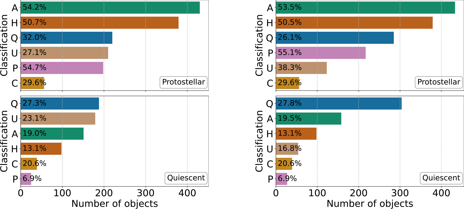
, with the best silhouette score (0.68) at a minimum cluster size of 75 and sample size of 45. We show the most stable clusters content in the left panel of Fig. 1. The former cluster is dominated by protostars and HII regions, while the latter cluster contain mainly IR-quiescent and uncertain clumps. Feature analysis with RF showed
 $\mathrm{C}_{2}\mathrm{H}$
and
 $\mathrm{N}_{2}\mathrm{H}^{+}$
as the most important molecular lines to identify the clusters. Our result is reasonable since
 $\mathrm{C}_{2}\mathrm{H}$
traces UV-irradiated gas and
 $\mathrm{N}_{2}\mathrm{H}^{+}$
is the tracer of dense gas. Adding 870
 $\mu$
m flux had negligible impact, confirming clustering stability.
Distribution of clump categories in the two most stable HDBSCAN clusters from t-SNE on five molecular lines (
 $\mathrm{HCO}^{+}$
, HNC,
 ${\mathrm{N}_{2}\mathrm{H}^{+}}$
, HCN,
 $\mathrm{C}_{2}\mathrm{H}$
). Bars show MALT90 classification (Q, A, C, H, P, U); percentages give fractions and numbers show counts. Left panel: before classification of uncertain clumps. Right panel: after classification.

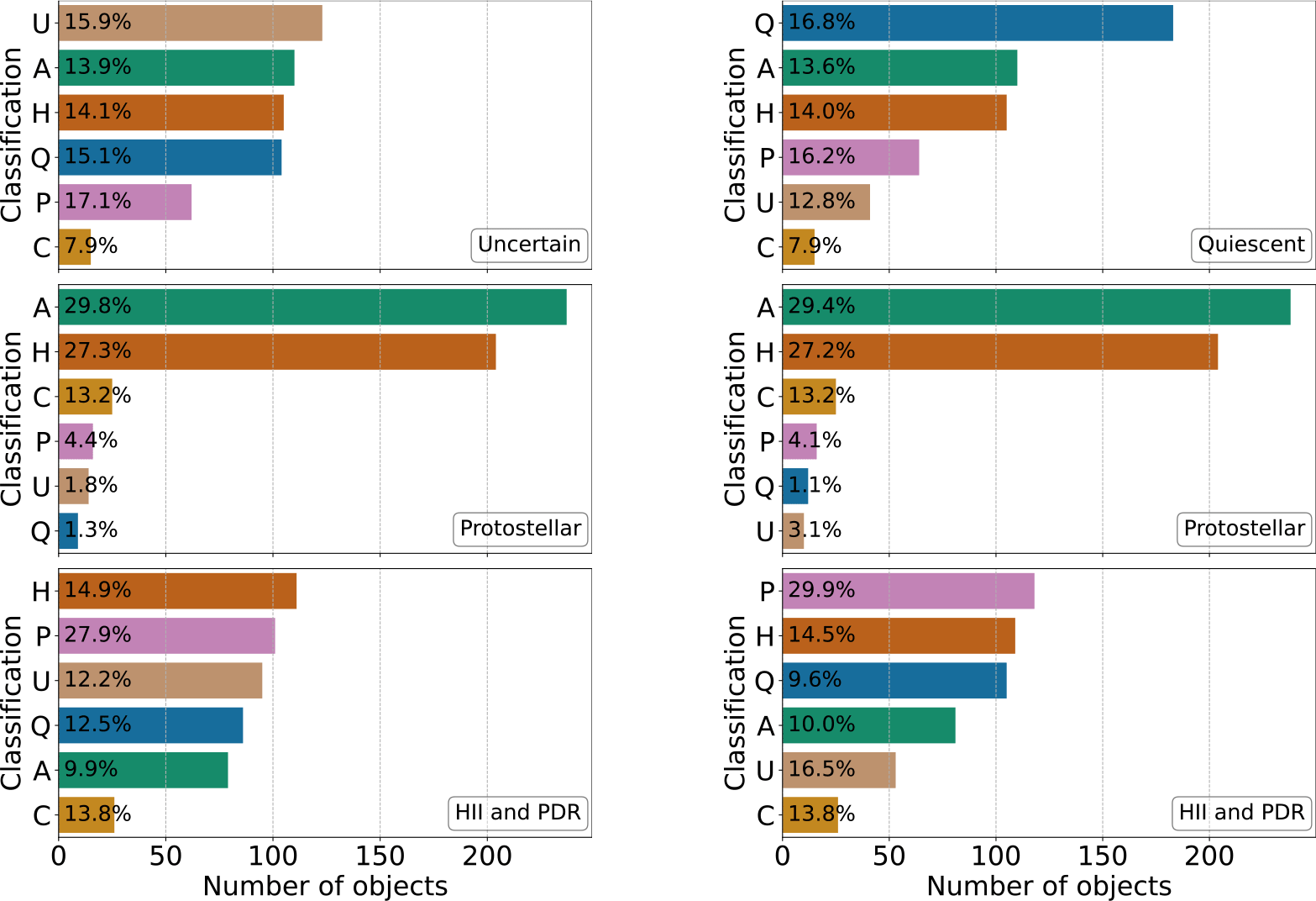
Following analysis of the clustering was performed using integrated intensities of 16 molecular lines, Spitzer infrared fluxes, and maser detection flags. The best silhouette score (0.65) was obtained with t-SNE perplexity 100, minimum cluster size 100, and minimum samples 50. As shown in the left panel of Fig. 2, the first cluster is dominated by the objects of the uncertain category, the second one – by protostars and HII regions, and the third one – by HII regions and PDRs. The most influential features were maser presence,
 $\mathrm{N}_{2}\mathrm{H}^{+}$
, and
 $\mathrm{C}_{2}\mathrm{H}$
.
Distribution of clump classes in the two most stable HDBSCAN clusters from t-SNE on sixteen molecular lines (
 $\mathrm{HCO}^{+}$
, HNC,
 ${\mathrm{N}_{2}\mathrm{H}^{+}}$
, HCN,
 $\mathrm{C}_{2}\mathrm{H}$
,
 $\mathrm{H}^{1}{3}\mathrm{CO}^{+}$
,
 $\mathrm{HN}^{1}{3}\mathrm{C}$
,
 $^{1}3\mathrm{CS}$
,
 $^{1}3\mathrm{C}^{3}4\mathrm{S}$
,
 $\mathrm{HC}^{1}3\mathrm{CCN}$
, HNCO,
 $\mathrm{CH}_{3}\mathrm{CN}$
,
 $\mathrm{HC}_{3}\mathrm{N}$
, HNCO, H 41
 $\alpha$
. Left panel: before classification of uncertain clumps. Right panel: after classification.

5.2. Classification results
Over 20% of MALT90 sources were labelled as uncertain by Rathborne et al. (Reference Rathborne, Whitaker, Jackson, Foster, Contreras, Stephens, Guzmán, Longmore, Sanhueza, Schuller, Wyrowski and Urquhart2016). To refine them, we applied RF and GB classifiers using 16 molecular lines and IR features. Both showed modest accuracy (
 $\sim0.6$
). With a 50% threshold, RF reassigned 527/774 clumps and GB 611/774, with 505 consistent between models and only 6 in disagreement. About 80% were IR-quiescent. Notably, IR fluxes, previously low-ranked, emerged as key predictors.
Next, we replaced uncertain category with classifications from the RF and GB models and repeated clustering. Results are shown in the right panels of Fig. 1 and Fig. 2. Quiescent-dominated clusters became more distinct, while protostar- and HII+PDR-dominated clusters remained stable, enhancing cluster homogeneity and evolutionary trends.
It was noted by Rathborne et al. (Reference Rathborne, Whitaker, Jackson, Foster, Contreras, Stephens, Guzmán, Longmore, Sanhueza, Schuller, Wyrowski and Urquhart2016) that there are plans to refine object classifications, including the use of maser emission. As shown in Fig. 2, adding class II methanol maser flags improved cluster separation and highlighted a protostar-dominated cluster.
6. Conclusion
This study analyzes clustering and classification of MALT90 molecular clumps. Using five molecular lines (
 $\mathrm{HCO}^{+}$
, HNC,
 ${\mathrm{N}_{2}\mathrm{H}^{+}}$
, HCN,
 $\mathrm{C}_{2}\mathrm{H}$
) separates protostellar and IR-quiescent clumps, while including IR fluxes (3.6–24
 $\mu$
), all 16 integtrted line intensities, and class II
 $\mathrm{CH}_{3}\mathrm{OH}$
masers reveals an additional cluster dominated by PDRs and HII regions. Clusters contained mixed MALT90 types, reflecting subjective IR-based classifications or continuous clump evolution. Random Forest and Gradient Boosting classified over 500 previously uncertain clumps, finding
 $\sim80\%$
quiescent. The two algorithms largely agreed, with only six discrepancies, mainly between protostars and quiescent clumps.
 HCO+
 N2H+
 C2H
 HCO+
 N2H+
 C2H
 H13CO+
 HN13C
 13CS
 13C34S
 HC13CCN
 CH3CN
 HC3N
 α


