1 Introduction
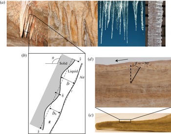
Falling film hydrodynamics can interact with a solid substrate and induce formidable geomorphic patterns, such as ice ripples, ice stalactites, draperies and crenulations (Meakin & Jamtveit Reference Meakin and Jamtveit2010; Camporeale & Ridolfi Reference Camporeale and Ridolfi2012a ,Reference Camporeale and Ridolfi b ; Chen & Morris Reference Chen and Morris2013; Camporeale Reference Camporeale2015). Crenulations are ring-like protuberances that develop on the surface of cave speleothems – namely stalactites, stalagmites or flowstones – under hydrodynamic-driven and geochemistry-driven conditions (figure 1). Several advancements in karst geochemistry have allowed understanding of the dependence of calcite precipitation rate on water chemistry and hydrodynamics, to model the shape evolution of speleothems (Romanov, Kaufmann & Dreybrodt Reference Romanov, Kaufmann and Dreybrodt2008). However, pattern formation of crenulations has been successfully modelled only recently, and a fully analytical treatment of the problem remains elusive. The analyses by Camporeale & Ridolfi (Reference Camporeale and Ridolfi2012b ) and Vesipa, Camporeale & Ridolfi (Reference Vesipa, Camporeale and Ridolfi2015) in fact require the numerical solution of an Orr–Sommerfeld-like problem, and previous attempts to develop a stability analysis with a simplified depth-averaged model (Dressler’s equations) failed the prediction of the crenulation formation (Chan & Goldenfeld Reference Chan and Goldenfeld2007). Therefore a closed form of the dispersion relation is not available yet. In the present work, it will be shown that a gradient expansion approach of Navier–Stokes equations, combined with a Kármán–Pohlhausen solution of the advection–diffusion equation for the calcium concentration, overcomes this limit, so a novel 1-D formulation is feasible and a fully analytical relationship for the wavelength selection is provided.
(a) Examples of ripple-like corrugations on cave stalactites and icicles. (b) Sketch of the physical schematization. (c) Longitudinal cut of a stalactite. (d) Evaluation of the slope factor
 $\unicode[STIX]{x1D6FD}$
. The arrow refers to the direction of the dripping water.

To achieve the aforementioned targets represents a considerable step forward in gap-bridging the theoretical efforts of geophysical fluid mechanics to the aims of karst sciences and to the search for new paleo-reconstruction techniques (Genty et al. Reference Genty, Blamart, Ouahdi, Gilmour, Baker, Jouzel and Van-Exter2003). In fact, although some properties of the speleothems (mineral composition, calcite crystals type, oxygen isotope values, etc.) can be statistically related to dripping water chemistry and to past environmental conditions, new methods are still invoked (Fairchild et al. Reference Fairchild, Smith, Baker, Fuller, Spotl, Mattey and McDermott2006). A rising interest in relating the geometry of geomorphic patterns to the flow features that have generated them suggests that easy-to-use relationships should be welcomed. In this perspective, Camporeale & Ridolfi (Reference Camporeale and Ridolfi2012a ) suggested the value of some morphometric quantities, such as the wavelength of crenulations and their phase velocity. In particular the phase velocity is related to an easily identifiable geometrical record – named slope factor – imprinted in the stalactite specimens. The slope factor is the angle between any constant-phase point of the wavelets, moving outward during the deposition process, and the normal-to-axis direction. This angle is visible on any longitudinal cut of a stalactite (an example is reported in figure 1 c,d). As it will be shown, the slope factor is highly sensitive to the flow conditions, so its recognition and modelling could provide a promising tool in paleo-climatology, based on paleo-crenulations. Through a formal theory, which is rigorous provided the Reynolds number is less than 1, the present paper goes in that direction.
2 Gradient expansion in a morphodynamic framework
It is a matter of fact that speleothems and the morphological patterns that occur over their surface, such as crenulations, develop at very low Reynolds numbers,
 $\mathit{Re}$
. By defining
 $\tilde{D}_{0}$
as the Nusselt solution of the film thickness under unperturbed conditions,
 $\tilde{U} _{0}$
the corresponding surface velocity and
 $\unicode[STIX]{x1D708}$
the kinematic viscosity of water, it holds that
 $\mathit{Re}=\tilde{U} _{0}\tilde{D}_{0}/\unicode[STIX]{x1D708}$
. Considering dripping waters in karst environments, where a single stalactite typically has a radius of 5–10 cm and it can perform a volumetric flow rate of water in the range
 $10^{-3}$
–1 litres per hour, it follows that
 $\mathit{Re}$
ranges in the interval
 $10^{-3}$
–1, which corresponds to a film thickness of
 $O(10)\,\unicode[STIX]{x03BC}\text{m}$
(Short, Baygents & Goldstein Reference Short, Baygents and Goldstein2005b
; Meakin & Jamtveit Reference Meakin and Jamtveit2010). Furthermore, the ratio
 $\unicode[STIX]{x1D716}$
of the film thickness to the pattern wavelength is also small (of the order of
 $10^{-3}$
) and the slope of the liquid–solid interface is close to
 $\unicode[STIX]{x1D703}=\unicode[STIX]{x03C0}/2$
(i.e. verticality, see figure 1). These peculiar conditions correspond to the drag-gravity regime, where inertia and surface tension do not change the basic velocity profile of the Nusselt solution in a significant way, thus allowing a long-wave modelling approach through the so-called gradient expansion (Kalliadasis et al.
Reference Kalliadasis, Ruyer-Quil, Scheid and Velarde2012). In the case of a film flowing over a rigid flat boundary, this technique leads to the well-known Benney equation and its weakly nonlinear versions, such as the Kawahara or Kuramoto–Sivashinsky equations (Pradas et al.
Reference Pradas, Pavliotis, Kalliadasis, Papageorgiou and Tseluiko2012). The Benney equation has been also extended to flows over corrugated boundaries (Tseluiko & Blyth Reference Tseluiko and Blyth2009; Tseluiko, Blyth & Papageorgiou Reference Tseluiko, Blyth and Papageorgiou2013).
In the present morphodynamic context, we instead need to extend the gradient expansion technique to the case where the lower boundary is also unknown and evolves with timescales very longer than hydrodynamics. Due to such a time-scale separation, it is therefore reasonable to neglect the hydrodynamic temporal modes (so-called surface and shear modes), since they do not affect the morphological evolution. The shear modes are not caught by a long-wave modelling but, since they are related to the turbulence transition, they are invariably stable at the present Reynolds numbers. The surface mode instead involves the free surface instability, and can be unstable even at low
 $\mathit{Re}$
for
 $\unicode[STIX]{x1D703}\sim \unicode[STIX]{x03C0}/2$
. However, this mode is characterized by surface waves migrating at velocities comparable to the flow velocity (
 $\text{mm}\,\text{s}^{-1}$
), while the migration rate of crenulations is of the order of centimetres per century. Therefore even the surface mode has no appreciable morphological consequences. For these reasons, the Navier–Stokes equations will be considered steady and the flow equations will be slaved to the evolution equation of the liquid–solid interface. This aspect can be quantitatively shown through an order of magnitude analysis, and is commonly referred to as the quasi-steady approximation (e.g. Camporeale & Ridolfi Reference Camporeale and Ridolfi2012b
).
2.1 Hydrodynamics
Let us adopt the Nusselt scales (
 $\tilde{D}_{0}$
,
 $\tilde{U} _{0}$
,
 $\unicode[STIX]{x1D70C}{\tilde{U} _{0}}^{2}$
) to non-dimensionalize lengths, velocities and pressure, respectively (
 $\unicode[STIX]{x1D70C}$
is water density). In addition, since the film thickness is normally much smaller than the radius of stalactite, curvature effects are completely negligible, and instead of an axisymmetric geometry, we will adopt a Cartesian one (e.g. Short et al.
Reference Short, Baygents, Beck, Stone, Toomey and Goldstein2005a
; Ueno et al.
Reference Ueno, Farzaneh, Yamaguchi and Tsuji2010). Accordingly, we define
 $x$
as the dimensionless downslope direction and
 $y$
the dimensionless normal to the unperturbed solid incline direction, while
 $u$
and
 $v$
are the corresponding velocities and
 $p$
is pressure (see figure 1
b). The spanwise direction is not consider here, since we will focus on cylindrical two-dimensional patterns. The elevations
 $y=\unicode[STIX]{x1D702}(x,t)$
and
 $y=\unicode[STIX]{x1D702}(x,t)+D(x,t)$
correspond to the liquid–solid interface and the free surface, respectively. After introducing a gradient expansion transformation of the type
 $(\unicode[STIX]{x2202}_{x},\unicode[STIX]{x2202}_{y},v)\rightarrow \unicode[STIX]{x1D716}(\unicode[STIX]{x2202}_{x},\unicode[STIX]{x2202}_{y},v)$
, the steady two-dimensional Navier–Stokes equations, truncated at order
 $\unicode[STIX]{x1D716}$
, read (Kalliadasis et al.
Reference Kalliadasis, Ruyer-Quil, Scheid and Velarde2012)
 $$\begin{eqnarray}\displaystyle & \displaystyle \unicode[STIX]{x1D716}\mathit{Re}(uu_{x}+vu_{y}+p_{x})=\unicode[STIX]{x1D716}^{2}u_{xx}+u_{yy}+2+O(\unicode[STIX]{x1D716}^{2}), & \displaystyle\end{eqnarray}$$
 $$\begin{eqnarray}\displaystyle & \displaystyle \mathit{Re}\,p_{y}=\unicode[STIX]{x1D716}v_{yy}-\unicode[STIX]{x1D6FF}+O(\unicode[STIX]{x1D716}^{2}), & \displaystyle\end{eqnarray}$$
 $$\begin{eqnarray}\displaystyle & u_{x}+v_{y}=0, & \displaystyle\end{eqnarray}$$
where subscripts refer to partial derivative and
 $\unicode[STIX]{x1D6FF}=2\cot \unicode[STIX]{x1D703}$
. The boundary conditions are
 $$\begin{eqnarray}\displaystyle & u=O(\unicode[STIX]{x1D716}^{2}),\quad (y=\unicode[STIX]{x1D702}) & \displaystyle\end{eqnarray}$$
 $$\begin{eqnarray}\displaystyle & v=O(\unicode[STIX]{x1D716}^{2}),\quad (y=\unicode[STIX]{x1D702}) & \displaystyle\end{eqnarray}$$
 $$\begin{eqnarray}\displaystyle & u_{y}=O(\unicode[STIX]{x1D716}^{2}),\quad (y=\unicode[STIX]{x1D702}+D) & \displaystyle\end{eqnarray}$$
 $$\begin{eqnarray}\displaystyle & p+\unicode[STIX]{x1D716}^{2}W(D_{xx}+\unicode[STIX]{x1D702}_{xx})-2\unicode[STIX]{x1D716}\mathit{Re}^{-1}v_{y}=O(\unicode[STIX]{x1D716}^{2}),\quad (y=\unicode[STIX]{x1D702}+D) & \displaystyle\end{eqnarray}$$
 $$\begin{eqnarray}\displaystyle & v-u(\unicode[STIX]{x1D702}_{x}+D_{x})=0\quad (y=\unicode[STIX]{x1D702}+D). & \displaystyle\end{eqnarray}$$
Equations (2.4) and (2.5) set no slip and impermeability at the lower boundary, respectively, (2.6) and (2.7) set the tangential and normal dynamic conditions at the free surface (
 $W=K\mathit{Re}^{-5/3}\sin \unicode[STIX]{x1D703}^{-1/3}$
is the Weber number,
 $K=5.77l_{c}^{2}\unicode[STIX]{x1D708}^{-4/3}$
is the Kapitza number and
 $l_{c}$
is the capillary length), while (2.8) is the (steady) kinematic condition at the free surface. This latter equation will be used as a solvability condition in what follows.
We seek the solution of the above hydrodynamic problem in the form
 $(u,v,p)=(u_{0},v_{0},p_{0})+\unicode[STIX]{x1D716}(u_{1},v_{1},p_{1})+O(\unicode[STIX]{x1D716}^{2})$
, taking into account the fact that
 $W$
is usually of the order of
 $\unicode[STIX]{x1D716}^{-2}$
(Kalliadasis et al.
Reference Kalliadasis, Ruyer-Quil, Scheid and Velarde2012).
At the order
 $O(\unicode[STIX]{x1D716}^{0})$
, we find
 $$\begin{eqnarray}u_{0,yy}=-2,\quad u_{0,x}+v_{0,y}=0,\quad p_{0,y}=-\unicode[STIX]{x1D6FF}/\mathit{Re},\;\qquad \;\;\end{eqnarray}$$
 $$\begin{eqnarray}u_{0}|_{\unicode[STIX]{x1D702}}=0,\quad v_{0}|_{\unicode[STIX]{x1D702}}=0,\quad u_{0,y}|_{\unicode[STIX]{x1D702}+D}=0,\quad p_{0}|_{D+\unicode[STIX]{x1D702}}=-W(h+\unicode[STIX]{x1D702})_{xx},\end{eqnarray}$$
with solutions
 $$\begin{eqnarray}\displaystyle & u_{0}=(y-\unicode[STIX]{x1D702})(2D-y+\unicode[STIX]{x1D702}), & \displaystyle\end{eqnarray}$$
 $$\begin{eqnarray}\displaystyle & v_{0}=(\unicode[STIX]{x1D702}-y)[(y-\unicode[STIX]{x1D702})D_{x}+(y-2D-\unicode[STIX]{x1D702})\unicode[STIX]{x1D702}_{x}], & \displaystyle\end{eqnarray}$$
 $$\begin{eqnarray}\displaystyle & \displaystyle p_{0}=\frac{\unicode[STIX]{x1D6FF}(D-y+\unicode[STIX]{x1D702})}{\mathit{Re}}-W(D+\unicode[STIX]{x1D702})_{xx}. & \displaystyle\end{eqnarray}$$
At the order
 $O(\unicode[STIX]{x1D716})$
we find
 $$\begin{eqnarray}u_{1,yy}=\mathit{Re}(p_{0,x}+u_{0}u_{0,x}+v_{0}u_{0,y}),\quad u_{1,x}+v_{1,y}=0,\end{eqnarray}$$
 $$\begin{eqnarray}u_{1}|_{\unicode[STIX]{x1D702}}=0,\quad v_{1}|_{\unicode[STIX]{x1D702}}=0,\quad u_{1,y}|_{\unicode[STIX]{x1D702}+D}=0,\end{eqnarray}$$
the solution thereof is
 $$\begin{eqnarray}\displaystyle \frac{u_{1}}{\mathit{Re}} & = & \displaystyle D\left[\frac{8g_{0}}{3}D^{3}+2D^{2}g_{1}+g_{2}D+\frac{g_{3}}{6}\right]\frac{\unicode[STIX]{x2202}D}{\unicode[STIX]{x2202}x}+\frac{3g_{1}}{2}\left[\frac{\unicode[STIX]{x1D6FF}}{\mathit{Re}}\frac{\unicode[STIX]{x2202}}{\unicode[STIX]{x2202}x}-W\frac{\unicode[STIX]{x2202}^{3}}{\unicode[STIX]{x2202}x^{3}}\right](\unicode[STIX]{x1D702}+D)\nonumber\\ \displaystyle & & \displaystyle +\,D\left[\frac{g_{0}\unicode[STIX]{x1D6FF}}{\mathit{Re}}\frac{\unicode[STIX]{x2202}\unicode[STIX]{x1D702}}{\unicode[STIX]{x2202}x}-g_{0}W\frac{\unicode[STIX]{x2202}^{3}}{\unicode[STIX]{x2202}x^{3}}(D+\unicode[STIX]{x1D702})\right],\end{eqnarray}$$
where
 $$\begin{eqnarray}g_{0}=y\unicode[STIX]{x1D702}-1;\quad g_{1}=y^{2}+y\unicode[STIX]{x1D702}^{2}-2\unicode[STIX]{x1D702};\quad g_{2}=\left(2y^{2}\unicode[STIX]{x1D702}+{\textstyle \frac{2}{3}}y\unicode[STIX]{x1D702}^{3}-2\unicode[STIX]{x1D702}^{2}-{\textstyle \frac{2}{3}}y^{3}\right),\end{eqnarray}$$
 $$\begin{eqnarray}g_{3}=y^{4}+\unicode[STIX]{x1D702}\left[\unicode[STIX]{x1D702}(6y^{2}+\unicode[STIX]{x1D702}(y\unicode[STIX]{x1D702}-4))+\frac{6y\unicode[STIX]{x1D6FF}}{\mathit{Re}}-4y^{3}\right]-\frac{6\unicode[STIX]{x1D6FF}}{\mathit{Re}}.\end{eqnarray}$$
Incidentally, we notice that the solution of
 $p_{1}$
is not needed for the following linear analysis. The complete solution of
 $v_{1}$
is cumbersome, and for the sake of space is not reported, but it suffices to emphasize that it is given in terms of the film thickness, the bottom elevation and their derivatives. Therefore, by using a shorthand notation, we can write
 $u_{0}+\unicode[STIX]{x1D716}u_{1}={\mathcal{U}}[D,\unicode[STIX]{x1D702}]$
and
 $v_{0}+\unicode[STIX]{x1D716}v_{1}={\mathcal{V}}[D,\unicode[STIX]{x1D702}]$
, where
 ${\mathcal{U}}$
and
 ${\mathcal{V}}$
are differential operators. The solutions of the flow field can be substituted into the kinematic condition (2.8) truncated at order
 $\unicode[STIX]{x1D716}$
. If we perturb the film thickness and the interface according to
 $D=1+d(x)$
and
 $\unicode[STIX]{x1D702}=\unicode[STIX]{x1D702}_{0}(t)+\unicode[STIX]{x1D709}(x,t)$
and linearize the resulting equation around the basic set
 $(D,\unicode[STIX]{x1D702})=(1,\unicode[STIX]{x1D702}_{0})$
, with
 $\unicode[STIX]{x1D702}_{0}\rightarrow 0$
and
 $\unicode[STIX]{x1D702}_{0,t}\neq 0$
for
 $t\rightarrow 0$
, one obtains
 $$\begin{eqnarray}{\mathcal{V}}[1,0;\unicode[STIX]{x1D716}]+\frac{\unicode[STIX]{x1D6FF}{\mathcal{V}}}{\unicode[STIX]{x1D6FF}D}d+\frac{\unicode[STIX]{x1D6FF}{\mathcal{V}}}{\unicode[STIX]{x1D6FF}\unicode[STIX]{x1D702}}\unicode[STIX]{x1D709}-{\mathcal{U}}[1,0;\unicode[STIX]{x1D716}]\left(\frac{\unicode[STIX]{x2202}d}{\unicode[STIX]{x2202}d}+\frac{\unicode[STIX]{x2202}\unicode[STIX]{x1D709}}{\unicode[STIX]{x2202}d}\right)=0,\end{eqnarray}$$
where functional derivation has been used. Since
 ${\mathcal{V}}[1,0;\unicode[STIX]{x1D716}]=0$
and
 ${\mathcal{U}}[1,0;\unicode[STIX]{x1D716}]=1$
, after straightforward algebra the ultimate hydrodynamic equation is obtained
 $$\begin{eqnarray}d-\unicode[STIX]{x1D716}\frac{\unicode[STIX]{x2202}}{\unicode[STIX]{x2202}x}\left[5\left(\unicode[STIX]{x1D6FF}-\mathit{Re}\,W\frac{\unicode[STIX]{x2202}^{2}}{\unicode[STIX]{x2202}x^{2}}\right)\frac{d+\unicode[STIX]{x1D709}}{12}-\frac{19\mathit{Re}}{60}d\right]=0.\end{eqnarray}$$
It should be noted that the perturbation of the flow depth has been assumed to be independent of time, by virtue of the quasi-steady approximation.
2.2 Kármán–Pohlhausen solution of calcium concentration
The calcium distribution is a key factor for the geochemistry of dripping waters, since its degree of supersaturation dictates the precipitation–dissolution rate (Dreybrodt Reference Dreybrodt1988). In order to develop a successful strategy able to foresee the pattern formation correctly, it is essential to model the calcium dynamics in a consistent way.
Basically, the flux of calcium at the free surface is zero, while at the interface it matches the rate of calcium precipitation in the form of calcium carbonate (calcite). Calcium concentration is normalized with a typical value
 $C_{0}$
(in
 $\text{mol}\,\text{kg}^{-1}$
), which will be further characterized in the following, and time is rescaled according to
 $\unicode[STIX]{x1D70F}=\unicode[STIX]{x1D712}t$
, with
 $\unicode[STIX]{x1D712}=C_{0}\unicode[STIX]{x1D71A}/\mathit{Pe}$
, where
 $\unicode[STIX]{x1D71A}$
is the molar volume of calcite,
 $\mathit{Pe}=\mathit{Re}\,\mathit{Pr}$
the Peclet number and
 $\mathit{Pr}$
the Prandtl number (i.e. the ratio between viscosity and calcium diffusivity). The diffusion–advection equation for the dimensionless calcium distribution,
 $C(x,y,\unicode[STIX]{x1D70F})$
, reads
 $$\begin{eqnarray}AC_{\unicode[STIX]{x1D70F}}+\unicode[STIX]{x1D716}\mathit{Pe}(uC_{x}+vC_{y})=C_{yy}+O(\unicode[STIX]{x1D716}^{2}),\end{eqnarray}$$
where
 $A=C_{0}\unicode[STIX]{x1D71A}$
. The boundary conditions to be set arise from the mass conservation imposed at the bottom and free surface respectively. Following a standard approach in continuum mechanics (Hutter Reference Hutter1983), the jump of the flux of calcium across the surface must be null, which in the present dimensionless notation reads
 $[\![(AC(\boldsymbol{u}-\boldsymbol{V})-\unicode[STIX]{x1D735}C)\boldsymbol{\cdot }\boldsymbol{n}]\!]=0$
, where
 $\boldsymbol{V}$
is the velocity of the surface,
 $\boldsymbol{n}$
is its normal versor and the brackets refer to the finite jump across the surface. After posing
 $\boldsymbol{u}=0$
at the solid bottom, setting to zero the flux of calcium through the air, recalling that
 $C=A^{-1}$
within the solid and using the quasi-steady approximation for the free surface variation, for weakly perturbed surfaces, we obtain
 $$\begin{eqnarray}C_{y}|_{\unicode[STIX]{x1D702}}=(1-AC)\unicode[STIX]{x1D702}_{\unicode[STIX]{x1D70F}},\quad C_{y}|_{D+\unicode[STIX]{x1D702}}=0.\end{eqnarray}$$
It should be noticed that the term proportional to
 $AC$
takes into account the fact that the surface is moving, as a consequence of the jump condition, and it has never been recognized in the previous works.
Before looking for a solution to (2.21) and (2.22), it is convenient to rectangularize the domain by introducing the normalized coordinate
 $\unicode[STIX]{x1D701}=(y-\unicode[STIX]{x1D702})/D(x,\unicode[STIX]{x1D70F})$
, from which
 $\unicode[STIX]{x2202}_{x}\rightarrow \unicode[STIX]{x2202}_{x}-D^{-1}(\unicode[STIX]{x1D701}D_{x}+\unicode[STIX]{x1D702}_{x})\unicode[STIX]{x2202}_{\unicode[STIX]{x1D701}}$
and
 $\unicode[STIX]{x2202}_{\unicode[STIX]{x1D70F}}\rightarrow \unicode[STIX]{x2202}_{\unicode[STIX]{x1D70F}}-D^{-1}(\unicode[STIX]{x1D701}D_{\unicode[STIX]{x1D70F}}+\unicode[STIX]{x1D702}_{\unicode[STIX]{x1D70F}})\unicode[STIX]{x2202}_{\unicode[STIX]{x1D701}}$
follows.
We are free to find the solution under the form
 $$\begin{eqnarray}C=1+G(\unicode[STIX]{x1D70F})g(\unicode[STIX]{x1D701})+\unicode[STIX]{x1D716}c_{1}(x,\unicode[STIX]{x1D701},\unicode[STIX]{x1D70F}),\end{eqnarray}$$
where the unknown functions
 $g(\unicode[STIX]{x1D701})$
and
 $G(\unicode[STIX]{x1D70F})$
account for the spatio-temporal dynamics of the basic state. At the order
 $O(\unicode[STIX]{x1D716}^{0})$
, equations (2.21) and (2.22) reduce to
 $$\begin{eqnarray}\displaystyle & \displaystyle \frac{g_{\unicode[STIX]{x1D701}\unicode[STIX]{x1D701}}}{g}=A\frac{G_{\unicode[STIX]{x1D70F}}}{G}=K, & \displaystyle\end{eqnarray}$$
 $$\begin{eqnarray}\displaystyle & {\mathcal{F}}_{0}[A+AgG-1]+Gg_{\unicode[STIX]{x1D701}}=0,\quad (\unicode[STIX]{x1D701}=0,\unicode[STIX]{x1D70F}=0) & \displaystyle\end{eqnarray}$$
 $$\begin{eqnarray}\displaystyle & g_{\unicode[STIX]{x1D701}}=1,\quad (\unicode[STIX]{x1D701}=1), & \displaystyle\end{eqnarray}$$
where
 $K$
is a constant to determine and
 ${\mathcal{F}}_{0}=\unicode[STIX]{x1D702}_{0,\unicode[STIX]{x1D70F}}$
is the overall rate of deposition of the interface that will be computed in the following. If the initial condition
 $G(0)=1$
is also set, the solution of the problem (2.24)–(2.26) reads
 $$\begin{eqnarray}g=\frac{(A-1){\mathcal{F}}_{0}\text{e}^{-\sqrt{K}(\unicode[STIX]{x1D701}+1)}(\text{e}^{2\unicode[STIX]{x1D701}\sqrt{K}}+\text{e}^{2\sqrt{K}})}{2(\sqrt{K}\sinh \sqrt{K}-A{\mathcal{F}}_{0}\cosh \sqrt{K})},\quad G=\text{e}^{K\unicode[STIX]{x1D70F}/A}.\end{eqnarray}$$
In order to complete the characterization of the basic state we still need to evaluate the constant
 $K$
. A reasonable strategy is to set the scale
 $C_{0}$
as the value of calcium concentration at
 $\unicode[STIX]{x1D701}=0$
. From this choice it follows that
 $g(0)=0$
, which is an implicit equation for
 $K$
. An approximate solution of this latter equation can be obtained by recalling that
 $A$
is usually small (e.g.
 $A\sim 10^{-4}\ll \sqrt{\unicode[STIX]{x1D716}}$
), so a first-order expansion of (2.27a
) provides
 $$\begin{eqnarray}\frac{{\mathcal{F}}_{0}\coth \sqrt{K}}{K}[(A-1)\sqrt{K}-A{\mathcal{F}}_{0}\coth \sqrt{K}]+O(A^{2})=0,\end{eqnarray}$$
thereof the only solution is
 $K=-\unicode[STIX]{x03C0}^{2}/4$
. From these considerations it follows that the (dimensionless) temporal scale
 $A/K$
is of the order of
 $10^{-5}$
, whereas it will be shown in what follows that the crenulation instability develops very slowly, e.g. at
 $\unicode[STIX]{x1D70F}\sim 10^{7}$
. This implies that the function
 $G(\unicode[STIX]{x1D70F})$
characterizing the temporal evolution of the basic scale vanishes before the triggering of the instability. This aspect justifies the adoption of the ansatz
 $C=1+\unicode[STIX]{x1D716}c_{1}(x,\unicode[STIX]{x1D701},\unicode[STIX]{x1D70F})$
in place of (2.23), a choice that was also used in the previous works, but without a rigorous justification. Taking into account the above arguments, the problem (2.21)–(2.22) at order
 $O(\unicode[STIX]{x1D716})$
reads
 $$\begin{eqnarray}A\frac{\unicode[STIX]{x2202}c_{1}}{\unicode[STIX]{x2202}\unicode[STIX]{x1D70F}}-\mathit{Pe}(\unicode[STIX]{x1D701}-2)\unicode[STIX]{x1D701}\frac{\unicode[STIX]{x2202}c_{1}}{\unicode[STIX]{x2202}x}-\frac{\unicode[STIX]{x2202}^{2}c_{1}}{\unicode[STIX]{x2202}\unicode[STIX]{x1D701}^{2}}=0,\end{eqnarray}$$
 $$\begin{eqnarray}\left.\frac{\unicode[STIX]{x2202}c_{1}}{\unicode[STIX]{x2202}\unicode[STIX]{x1D701}}\right|_{0}=(1-A)\frac{\unicode[STIX]{x2202}\unicode[STIX]{x1D709}}{\unicode[STIX]{x2202}t}-A{\mathcal{F}}_{0}c_{1},\quad \left.\frac{\unicode[STIX]{x2202}c_{1}}{\unicode[STIX]{x2202}\unicode[STIX]{x1D701}}\right|_{1}=0.\end{eqnarray}$$
It is instructive to provide two different solutions of the above problem, namely the exact one and an approximate one. The exact solution is achieved by posing
 $\{c_{1},\unicode[STIX]{x1D709}\}=\{{\hat{c}}_{1}(\unicode[STIX]{x1D701}),\hat{\unicode[STIX]{x1D709}}\}\text{e}^{\text{i}kx+\unicode[STIX]{x1D706}t}$
, which provides a parabolic cylinder differential problem
 $$\begin{eqnarray}{\hat{c}}_{1}^{\prime \prime }+[\text{i}k\mathit{Pe}(\unicode[STIX]{x1D701}-2)\unicode[STIX]{x1D701}-A\unicode[STIX]{x1D706}]{\hat{c}}_{1}=0,\end{eqnarray}$$
 $$\begin{eqnarray}{\hat{c}}_{1}^{\prime }(0)=(1-A)\unicode[STIX]{x1D706}-A{\mathcal{F}}_{0}{\hat{c}}_{1}(0),\quad {\hat{c}}_{1}^{\prime }(1)=0.\end{eqnarray}$$
The solution of (2.31)–(2.32) is provided in terms of special functions and it is quite cumbersome. As will be clear in the next section, we just need to compute its value at the solid bottom, i.e.
 ${\hat{c}}_{1}(0)$
, and, since
 $\unicode[STIX]{x1D706}\ll 1$
(see later), a solution to the lowest order in
 $\unicode[STIX]{x1D706}$
is
 $$\begin{eqnarray}\displaystyle {\hat{c}}_{1}(0)\sim \frac{\sqrt{2}(A-1)\unicode[STIX]{x1D706}(2^{s}{\mathcal{D}}_{-s-(1/2)}^{2\text{i}\sqrt{2}s}\unicode[STIX]{x1D6E4}_{(1/4)-(\text{i}s/2)}+\text{i}{\mathcal{D}}_{s-(1/2)}^{-2\sqrt{2}s}\unicode[STIX]{x1D6E4}_{(1/4)-(s/2)})}{\unicode[STIX]{x1D6E4}_{(1/4)-(s/2)}(p{\mathcal{D}}_{s-(1/2)}^{-2\sqrt{s}}-q{\mathcal{D}}_{s+(1/2)}^{-2\sqrt{s}})+2^{s+(1/2)}{\mathcal{D}}_{-s-(1/2)}^{2\text{i}\sqrt{s}}\unicode[STIX]{x1D6E4}_{(1/4)-(\text{i}s/2)}(A{\mathcal{F}}_{0}+2s)+2^{s}q{\mathcal{D}}_{(1/2)-s}^{2\text{i}\sqrt{s}}\unicode[STIX]{x1D6E4}_{(1/4)-(\text{i}s/2)}}, & & \displaystyle \nonumber\\ \displaystyle & & \displaystyle\end{eqnarray}$$
where
 $p=\sqrt{2}\text{i}A{\mathcal{F}}_{0}+(1+\text{i})\sqrt{k\mathit{Pe}}$
and
 $q=4\text{i}^{7/4}k\mathit{Pe}$
,
 $s=\sqrt{\text{i}k\mathit{Pe}}/2$
, whereas
 ${\mathcal{D}}_{a}^{b}\equiv {\mathcal{D}}_{\unicode[STIX]{x1D708}}(b)$
is a shorthand notation for the parabolic cylinder function, and
 $\unicode[STIX]{x1D6E4}_{a}\equiv \unicode[STIX]{x1D6E4}(a)$
refers to the Gamma function (Abramowitz & Stegun Reference Abramowitz and Stegun1972).
The solution (2.33) is of little practical utility for the presence of the special functions, which are not explicit in
 $k$
. Therefore, it is convenient to address the solution of (2.29) in an alternative approximate way. We will use a Kármán–Pohlhausen approach by setting
 $c_{1}=\unicode[STIX]{x1D719}(x,\unicode[STIX]{x1D70F})+a_{0}\unicode[STIX]{x1D701}+a_{1}\unicode[STIX]{x1D701}^{2}$
, where
 $\unicode[STIX]{x1D719}$
is still unknown and
 $a_{i}=a_{i}(x,\unicode[STIX]{x1D70F})$
are obtained by using (2.30), hence
 $$\begin{eqnarray}c_{1}=\unicode[STIX]{x1D719}+\left[(A-1)\unicode[STIX]{x1D709}_{\unicode[STIX]{x1D70F}}-A{\mathcal{F}}_{0}\unicode[STIX]{x1D719}\right]\unicode[STIX]{x1D701}-{\textstyle \frac{1}{2}}[(A-1)\unicode[STIX]{x1D709}_{\unicode[STIX]{x1D70F}}-A{\mathcal{F}}_{0}\unicode[STIX]{x1D719}]\unicode[STIX]{x1D701}^{2}.\end{eqnarray}$$
Notice that the value of the (dimensionless) calcium concentration at the wall is given by
 $C(0)=1+\unicode[STIX]{x1D716}\unicode[STIX]{x1D719}$
.
By substituting (2.34) into (2.29), and depth integrating, we arrive at
 $$\begin{eqnarray}\frac{{\mathcal{F}}_{0}}{A-1}\left[15A+5A^{2}\frac{\unicode[STIX]{x2202}}{\unicode[STIX]{x2202}\unicode[STIX]{x1D70F}}+4AP\frac{\unicode[STIX]{x2202}}{\unicode[STIX]{x2202}x}\right]\unicode[STIX]{x1D719}-\left[15+4(A-1)P\frac{\unicode[STIX]{x2202}}{\unicode[STIX]{x2202}x}+5A(A-1)\frac{\unicode[STIX]{x2202}}{\unicode[STIX]{x2202}\unicode[STIX]{x1D70F}}\right]\frac{\unicode[STIX]{x2202}\unicode[STIX]{x1D709}}{\unicode[STIX]{x2202}\unicode[STIX]{x1D70F}}=0.\end{eqnarray}$$
By posing again a plane wave structure
 $\unicode[STIX]{x1D719}=\hat{\unicode[STIX]{x1D719}}\text{e}^{\text{i}kx+\unicode[STIX]{x1D706}t}$
, the above equation provides the approximate value of
 ${\hat{c}}_{1}(0)\equiv \hat{\unicode[STIX]{x1D719}}$
,
 $$\begin{eqnarray}\hat{\unicode[STIX]{x1D719}}=\frac{(1-A)\unicode[STIX]{x1D706}(5A\unicode[STIX]{x1D706}+4\text{i}kP+15)}{5A[3\unicode[STIX]{x1D706}-{\mathcal{F}}_{0}(A\unicode[STIX]{x1D706}+3)]+2\text{i}kP(5-2A{\mathcal{F}}_{0})}.\end{eqnarray}$$
In the following, we will compare the two solutions (2.33) and (2.36) in terms of the performance on the stability analysis, in order to test the Kármán–Pohlhausen approximation (2.34).
2.3 The evolution equation for the liquid–solid interface
The evolution of the liquid–solid interface is driven by three rate-limited reactions involving calcite, carbon dioxide, calcium and carbonate ions (Romanov et al. Reference Romanov, Kaufmann and Dreybrodt2008), whose overall stoichiometry can be summarized as

From (2.37), Plummer, Wigley & Parkhurst (Reference Plummer, Wigley and Parkhurst1978) derived the so-called PWP equation for the calcite flux. The PWP equation has been recently rearranged by Camporeale & Ridolfi (Reference Camporeale and Ridolfi2012a
) with the aid of the electroneutrality condition, the ionic product of water, the solubility product of calcite and two non-rate-limited reactions involving H2CO3,
 $\text{CO}_{3}^{2-}$
and
 $\text{HCO}_{3}^{-}$
. The result was an evolution equation in the form of
 $\unicode[STIX]{x1D702}_{\unicode[STIX]{x1D70F}}=n_{0}+n_{1}(1+\unicode[STIX]{x1D719})+n_{2}(1+\unicode[STIX]{x1D719})^{2}$
, where the coefficients
 $n_{i}$
are complicated functions of pH, temperature and the carbon dioxide concentration. Although this approach has led to a correct numerical evaluation of crenulation instability, we will follow a slight modification of the same rationale, which is based on the derivation by Short et al. (Reference Short, Baygents and Goldstein2005b
), who adopted the principle that the growth of the surface is related to the amount of carbon dioxide leaving the film into the atmosphere. In fact, from (2.37) for one mole of
 $\text{Ca}^{2+}$
dissolved, one mole of CO2 is taken from the solution and it must be replaced from the carbon dioxide in the atmosphere, as the system is open with respect to CO2 by the free surface. For the reader’s convenience, we will briefly sum up the derivation by Short et al. (Reference Short, Baygents and Goldstein2005b
) using our notation and with a few small changes. Let us start from the slowest chemical reactions involving CO2,


Two hypotheses are then necessary: (i) [
 $\text{H}^{+}$
] and [
 $\text{HCO}_{3}^{-}$
] are almost constant over the film, and (ii) longitudinal diffusion and advection of CO2 are negligible. We can use the same scaling of the previous section, and set the aqueous content of carbon dioxide to
 $[\text{CO}_{2}]={\mathcal{H}}C_{\infty }(1+\unicode[STIX]{x1D713}[x,\unicode[STIX]{x1D701},\unicode[STIX]{x1D70F}])$
, where
 ${\mathcal{H}}$
is Henry’s constant and
 $C_{\infty }$
is the atmospheric carbon dioxide concentration far from the stalactite. After computing the local production of carbon dioxide from (2.38) and (2.39), the reaction–diffusion equation reduces to
 $$\begin{eqnarray}\frac{\unicode[STIX]{x2202}^{2}\unicode[STIX]{x1D713}}{\unicode[STIX]{x2202}\unicode[STIX]{x1D701}^{2}}=D^{2}\unicode[STIX]{x1D6E5}(\unicode[STIX]{x1D713}-\unicode[STIX]{x1D714}),\end{eqnarray}$$
with
 $$\begin{eqnarray}\unicode[STIX]{x1D6E5}=\hat{\mathit{Pe}}(\hat{k}_{1}^{+}+\hat{k}_{2}^{+}[\text{OH}^{-}]),\quad \unicode[STIX]{x1D714}=\frac{(\hat{k}_{1}^{-}[\text{H}^{+}]+\hat{k}_{2}^{-})[\text{HCO}_{3}^{-}]}{(\hat{k}_{1}^{+}+\hat{k}_{2}^{+}[\text{OH}^{-}]){\mathcal{H}}C_{\infty }}-1,\end{eqnarray}$$
where
 $\hat{\mathit{Pe}}$
is the Peclet number related to the carbon dioxide diffusivity, this latter being equal to 1.42 times the calcium diffusivity (Romanov et al.
Reference Romanov, Kaufmann and Dreybrodt2008), while
 $\hat{k}_{i}^{\pm }=\tilde{D}_{0}k_{i}^{\pm }/\tilde{U} _{0}$
. Notice that with the aid of the electroneutrality condition, the ionic product of water and the solubility product of calcite, the quantities [
 $\text{HCO}_{3}^{-}$
] and [
 $\text{OH}^{-}$
] can be written in terms of
 $C_{0}$
and pH.
The concentration of the atmospheric carbon dioxide (
 $C_{a}$
) in proximity of the stalactite can be obtained from the diffusion equation written in cylindrical coordinates, with the solution
 $C_{a}=C_{\infty }+B/r\tilde{D}_{0}$
, where
 $r$
is the dimensionless distance from the centre of the stalactite and
 $B$
is a constant to be determined. It follows that
 $$\begin{eqnarray}\unicode[STIX]{x1D713}(1)=\frac{B}{RC_{\infty }\tilde{D}_{0}},\quad \tilde{{\mathcal{F}}}={\mathcal{D}}_{a}\frac{B}{R^{2}\tilde{D}_{0}^{2}}=-{\mathcal{D}}_{w}\frac{{\mathcal{H}}C_{\infty }}{D\tilde{D}_{0}}\left.\frac{\unicode[STIX]{x2202}\unicode[STIX]{x1D713}}{\unicode[STIX]{x2202}\unicode[STIX]{x1D701}}\right|_{1},\end{eqnarray}$$
where
 $R$
is the dimensionless radius of stalactite,
 $\tilde{{\mathcal{F}}}$
is the (dimensional) flux of CO2 leaving the film into the atmosphere and
 ${\mathcal{D}}_{a}$
and
 ${\mathcal{D}}_{w}$
are the atmospheric and aqueous diffusivity of carbon dioxide, respectively. After eliminating
 $B$
from (2.42) and setting to zero the flux of CO2 at the wall, one obtains the boundary conditions for (2.40):
 $$\begin{eqnarray}\left.\frac{\unicode[STIX]{x2202}\unicode[STIX]{x1D713}}{\unicode[STIX]{x2202}\unicode[STIX]{x1D701}}\right|_{1}=-\frac{{\mathcal{D}}_{a}D}{{\mathcal{D}}_{w}{\mathcal{H}}R}\unicode[STIX]{x1D713}(1),\quad \left.\frac{\unicode[STIX]{x2202}\unicode[STIX]{x1D713}}{\unicode[STIX]{x2202}\unicode[STIX]{x1D701}}\right|_{0}=0.\end{eqnarray}$$
By recalling that
 $\unicode[STIX]{x1D6E5}\ll 1$
, a solution of the problem (2.40), (2.43) to the lowest order in
 $\unicode[STIX]{x1D6E5}$
is
 $$\begin{eqnarray}\unicode[STIX]{x1D713}=\unicode[STIX]{x1D714}D\unicode[STIX]{x1D6E5}\left(D\frac{1-\unicode[STIX]{x1D701}^{2}}{2}+{\mathcal{H}}R\frac{{\mathcal{D}}_{w}}{{\mathcal{D}}_{a}}\right).\end{eqnarray}$$
At this point, it is sufficient to enforce that the dimensional calcite flux at the liquid–solid interface [
 $\text{mols}~\text{m}^{-2}~\text{s}^{-1}$
] matches the flux of carbon dioxide at the liquid–air interface. If we define the dimensionless flux as
 $\unicode[STIX]{x1D702}_{\unicode[STIX]{x1D70F}}\equiv {\mathcal{F}}=\tilde{{\mathcal{F}}}\mathit{Pe}/C_{0}\tilde{U} _{0}$
, after combining (2.42)–(2.43) and recalling that
 $D=1+d$
and the calcium concentration at the wall is
 $1+\unicode[STIX]{x1D716}\unicode[STIX]{x1D719}$
, we finally obtain
 $$\begin{eqnarray}\unicode[STIX]{x1D702}_{\unicode[STIX]{x1D70F}}=\unicode[STIX]{x1D6E4}(1+d)(1+\unicode[STIX]{x1D716}\unicode[STIX]{x1D719}-\unicode[STIX]{x1D705}),\end{eqnarray}$$
where
 $\unicode[STIX]{x1D6E4}$
and
 $\unicode[STIX]{x1D705}$
are complicated functions of
 $C_{0}$
,
 $\mathit{Re}$
,
 $\mathit{Pe}$
, CO2 partial pressure (
 $p_{c}$
) and temperature (see appendix A). Notice that the above derivation contains two variations with respect to the formulation by Short et al. (Reference Short, Baygents and Goldstein2005b
): (i) since we are considering the free surface perturbation, the factor
 $D^{2}$
appears in (2.40) and therefore the quantity
 $(1+d)$
appears in (2.45), which is a key linkage between the flow field and the bed evolution equation; (ii) in the formulation by Short et al. (Reference Short, Baygents and Goldstein2005b
) a cylindrical geometry was initially considered but, since
 $\tilde{D}_{0}\ll R$
, it was eventually recognized that the stalactite geometry is irrelevant and one can assume a local planar geometry, as we did.
Put in this form, the evolution equation resembles the most commonly used formulations (Dreybrodt Reference Dreybrodt1988) where the deposition rate is proportional to the degree of supersaturation, namely the difference between calcium concentration at the wall (
 $1+\unicode[STIX]{x1D716}\unicode[STIX]{x1D719}$
) and its saturated value
 $\unicode[STIX]{x1D705}$
. It can be shown that (2.45) is coherent to the PWP equation, but its explicit appearance of the depth perturbation,
 $d$
, makes it more suitable in the context of thin films. This aspect has been in fact decisive in formulating a theory for fluting formation (Camporeale Reference Camporeale2015). We finally notice that from (2.45) it follows that
 $\unicode[STIX]{x1D702}_{0,\unicode[STIX]{x1D70F}}\equiv {\mathcal{F}}_{0}=\unicode[STIX]{x1D6E4}(1-\unicode[STIX]{x1D705})$
.
3 Stability analysis and results
With the aim of addressing a linear stability analysis, let us recall the normal mode ansatz that we have already introduced above:
 $$\begin{eqnarray}\{d,\unicode[STIX]{x1D719},\unicode[STIX]{x1D709}\}=\{\hat{d},\hat{\unicode[STIX]{x1D719}},\hat{\unicode[STIX]{x1D709}}\}\exp [\text{i}kx+\unicode[STIX]{x1D706}\unicode[STIX]{x1D70F}]+\text{c.c.},\end{eqnarray}$$
where
 $k$
is the longitudinal wavenumber of the perturbation,
 $-{\mathcal{I}}[\unicode[STIX]{x1D706}]/k\equiv -\unicode[STIX]{x1D706}_{i}/k:=c_{p}$
is its phase velocity and
 ${\mathcal{R}}[\unicode[STIX]{x1D706}]\equiv \unicode[STIX]{x1D706}_{r}>0$
corresponds to the unstable conditions (c.c. refers to complex conjugate). Since the gradient expansion analysis served to identify the dominant terms in hydrodynamics and calcium dynamics, we can now set
 $\unicode[STIX]{x1D716}=1$
, without any loss of generality. By inserting (3.1) in (2.20), (2.35), (2.45), one obtains
 $$\begin{eqnarray}\displaystyle \!\left(\begin{array}{@{}ccc@{}}\unicode[STIX]{x1D706} & -{\mathcal{F}}_{0} & \unicode[STIX]{x1D6E4}\\ 25k^{2}\unicode[STIX]{x1D70C}_{0} & k\unicode[STIX]{x1D70C}_{1} & 0\\ \displaystyle \unicode[STIX]{x1D706}(1-A)\left(1+\frac{4\unicode[STIX]{x1D70C}_{2}}{15}+\frac{A\unicode[STIX]{x1D706}}{3}\right) & 0 & \displaystyle A\left({\mathcal{F}}_{0}+\frac{4{\mathcal{F}}_{0}\unicode[STIX]{x1D70C}_{2}}{15}-\unicode[STIX]{x1D706}\right)-\frac{2}{3}\unicode[STIX]{x1D70C}_{2}+\frac{1}{3}A^{2}{\mathcal{F}}_{0}\unicode[STIX]{x1D706}\end{array}\right)\cdot \left(\begin{array}{@{}c@{}}\hat{\unicode[STIX]{x1D709}}\\ \hat{d}\\ \hat{\unicode[STIX]{x1D719}}\end{array}\right)=0,\qquad & & \displaystyle\end{eqnarray}$$
where
 $\unicode[STIX]{x1D70C}_{0}=k^{2}\mathit{Re}\,W+\unicode[STIX]{x1D6FF}$
,
 $\unicode[STIX]{x1D70C}_{1}=60\text{i}+19k\,\mathit{Re}+25k^{3}\mathit{Re}\,W+25k\unicode[STIX]{x1D6FF}$
and
 $\unicode[STIX]{x1D70C}_{2}=\text{i}k\,\mathit{Pe}$
.
The above system allows non-trivial solutions if the determinant is set to zero. As a result, two solutions for
 $\unicode[STIX]{x1D706}$
are obtained, of which one is invariably stable, while the other one provides the first outcome of the present work, namely the dispersion relation in a closed form fashion
 $$\begin{eqnarray}\displaystyle \unicode[STIX]{x1D706} & = & \displaystyle \frac{{\mathcal{F}}_{0}(375\unicode[STIX]{x1D705}_{1}k\unicode[STIX]{x1D70C}_{0}-125A_{0}\unicode[STIX]{x1D705}_{1}k\unicode[STIX]{x1D70C}_{0}+10\unicode[STIX]{x1D705}\unicode[STIX]{x1D70C}_{1}\unicode[STIX]{x1D70C}_{4})}{10\unicode[STIX]{x1D70C}_{1}\unicode[STIX]{x1D70C}_{3}}-\frac{{\mathcal{F}}_{0}\unicode[STIX]{x1D70C}_{4}-\unicode[STIX]{x1D705}_{1}\unicode[STIX]{x1D70C}_{2}}{A\unicode[STIX]{x1D70C}_{3}}\nonumber\\ \displaystyle & & \displaystyle +\,\frac{\sqrt{[\unicode[STIX]{x1D705}_{1}(\unicode[STIX]{x1D70C}_{1}\unicode[STIX]{x1D70C}_{2}-25A_{0}k\unicode[STIX]{x1D70C}_{0}(A_{0}-3)/2)+\unicode[STIX]{x1D70C}_{1}\unicode[STIX]{x1D70C}_{4}(\unicode[STIX]{x1D70C}_{3}+3\unicode[STIX]{x1D705}_{1})]^{2}-5A_{0}\unicode[STIX]{x1D705}_{1}k\unicode[STIX]{x1D70C}_{0}\unicode[STIX]{x1D70C}_{1}\unicode[STIX]{x1D70C}_{3}(A_{0}\unicode[STIX]{x1D70C}_{4}-10\unicode[STIX]{x1D70C}_{2})}}{A\unicode[STIX]{x1D70C}_{1}\unicode[STIX]{x1D70C}_{3}},\nonumber\\ \displaystyle & & \displaystyle\end{eqnarray}$$
where
 $\unicode[STIX]{x1D705}_{1}=1-\unicode[STIX]{x1D705}$
,
 $\unicode[STIX]{x1D70C}_{3}={\mathcal{F}}_{0}(1-A\unicode[STIX]{x1D705})-3\unicode[STIX]{x1D705}_{1}$
,
 $\unicode[STIX]{x1D70C}_{4}=(15+4\unicode[STIX]{x1D70C}_{2})/10$
and
 $A_{0}=A{\mathcal{F}}_{0}$
. While using (A 1) one recognizes that
 $\unicode[STIX]{x1D6E4}\ll 1$
, so the above expression can be further simplified, by expanding in powers of
 $\unicode[STIX]{x1D6E4}$
, with the final result:
 $$\begin{eqnarray}\unicode[STIX]{x1D706}\sim \frac{5{\mathcal{F}}_{0}[\unicode[STIX]{x1D6E4}(1-A)(15\text{i}-4k\,\mathit{Pe})-10k\,\mathit{Pe}](\unicode[STIX]{x1D6FF}+k^{2}\mathit{Re}\,W)}{2\mathit{Pe}(25k^{3}\mathit{Re}\,W+25\unicode[STIX]{x1D6FF}k+19k\,\mathit{Re}+60\text{i})}+O(\unicode[STIX]{x1D6E4}^{2}).\end{eqnarray}$$
We remind the reader that the results (3.3)–(3.4) come from the Kármán–Pohlhausen solution. In order to test its validity we will use the exact solution (2.33) for the term
 $\hat{\unicode[STIX]{x1D719}}$
and, after repeating the linear stability analysis, we get
 $$\begin{eqnarray}\unicode[STIX]{x1D706}=\frac{25{\mathcal{F}}k(\unicode[STIX]{x1D6FF}+k^{2}\mathit{Re}\,W)}{(\unicode[STIX]{x1D6E4}{\mathcal{G}}(k,\mathit{Pe},C_{0})-1)(25k^{3}\mathit{Re}W+25\unicode[STIX]{x1D6FF}k+19k\,\mathit{Re}+60\text{i})},\end{eqnarray}$$
where the function
 ${\mathcal{G}}$
is the same appearing as that in the right-hand side of (2.33), but with
 $\unicode[STIX]{x1D706}$
set to 1.
In addition, since we are mainly interested in pattern formation on nearly vertical speleothems such as stalactites, the slope will be written in terms of its difference with respect to verticality, i.e.
 $\unicode[STIX]{x1D703}_{1}=\unicode[STIX]{x1D703}-\unicode[STIX]{x03C0}/2$
.

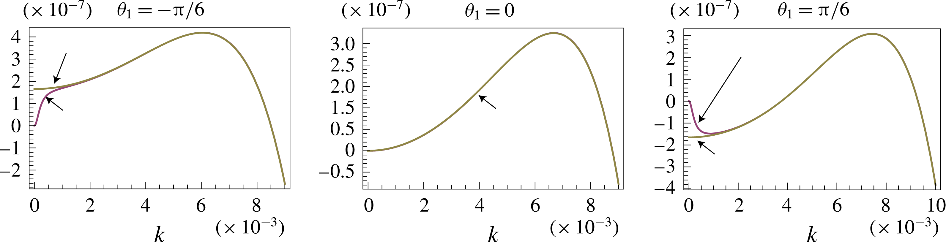
Figure 2 provides a comparison among (3.3), (3.4) and (3.5). The overlapping is almost complete, so testifying for the goodness of the Kármán–Pohlhausen approximation. The only exception is a slight deviation of the approximated (3.4) from the exact value at small wavenumbers, and only when
 $\unicode[STIX]{x1D703}_{1}\neq 0$
. However, such a deviation becomes completely negligible for the
 $k$
-values that maximize the dispersion relation. Therefore (3.4) is completely suitable for our purposes.
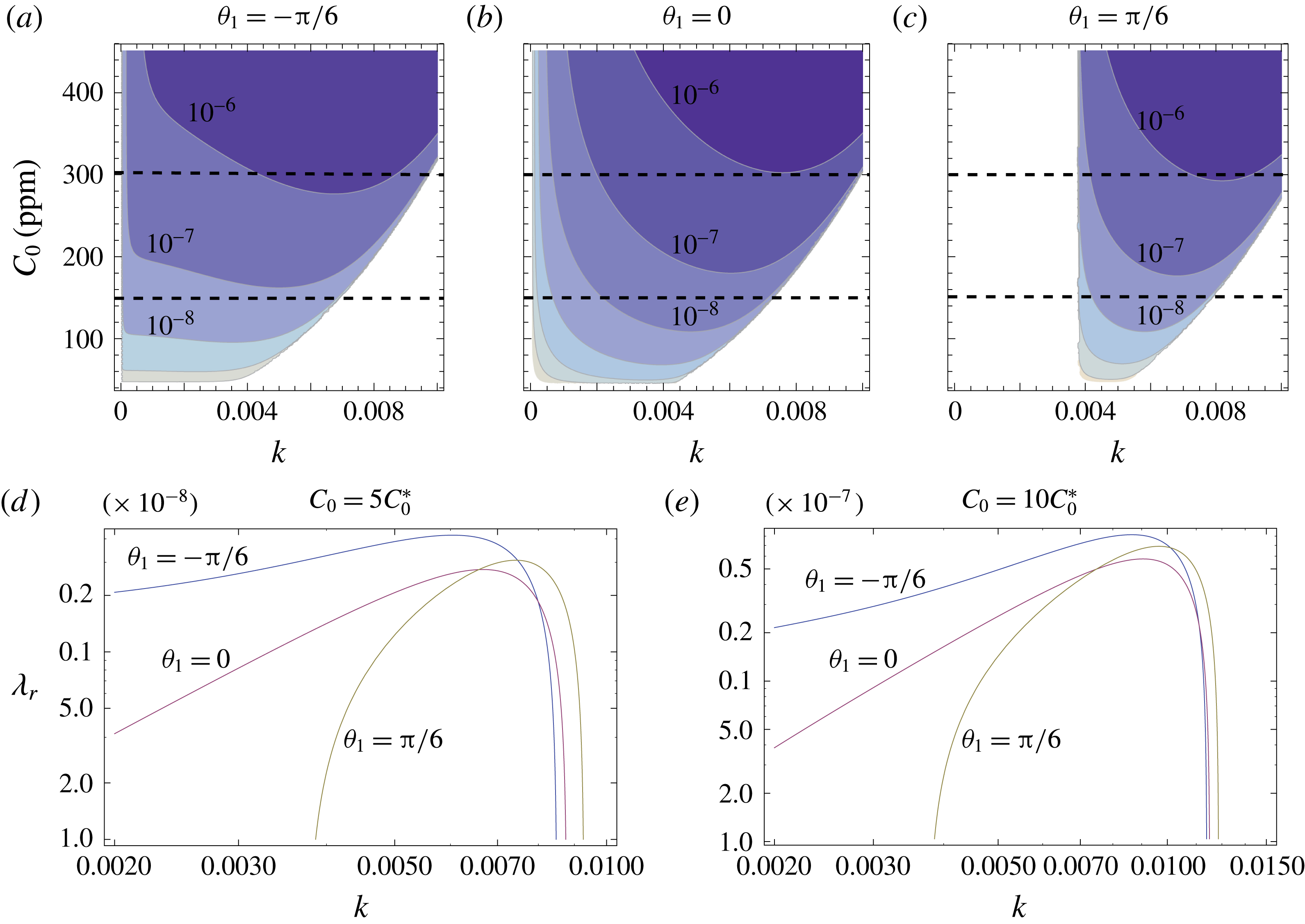
Figure 3 shows two representations of the results achievable from the dispersion relation (3.4) for the case
 $\mathit{Re}=0.01$
. The density plots reported in panels (a–c) show the effect of the slope
 $\unicode[STIX]{x1D703}_{1}$
: for normal slopes (
 $\unicode[STIX]{x1D703}_{1}\leqslant 0$
) there is only one upper cutoff in the wavenumber (
 $k=k_{u}$
), while for inverted flows (
 $\unicode[STIX]{x1D703}_{1}>0$
) a lower bound
 $k_{l}$
also appears, such that the flat base-state solution is unstable for
 $k_{l}<k<k_{u}$
. By setting the growth rate to zero (i.e.
 $\text{Re}[\unicode[STIX]{x1D706}]\equiv \unicode[STIX]{x1D706}_{r}=0$
), the solutions for these two bounds read
 $$\begin{eqnarray}\displaystyle & \displaystyle k_{l}^{2}=-\frac{\unicode[STIX]{x1D6FF}}{\mathit{Re }W}, & \displaystyle\end{eqnarray}$$
 $$\begin{eqnarray}\displaystyle & \displaystyle k_{u}\sim \frac{5\mathit{Pe}\,R^{5/6}\unicode[STIX]{x1D6FF}^{2}\unicode[STIX]{x1D708}^{5/3}-24\sqrt[3]{2}l_{c}(\sqrt[3]{2g}\sqrt{5}\unicode[STIX]{x1D6FF}\unicode[STIX]{x1D708}\sqrt{\unicode[STIX]{x1D70E}\mathit{Pe }\,\mathit{Re}}-24\sqrt[6]{\mathit{Re}}l_{c}\unicode[STIX]{x1D70E}\sqrt[3]{g^{2}\unicode[STIX]{x1D708}})}{560g^{5/6}l_{c}^{5/2}\sqrt{\unicode[STIX]{x1D70E}}\sqrt[4]{\mathit{Pe}\unicode[STIX]{x1D70E}}}, & \displaystyle\end{eqnarray}$$
where
 $\unicode[STIX]{x1D70E}=\unicode[STIX]{x1D6E4}(1-A)$
.
By recalling the definition of
 $\unicode[STIX]{x1D6FF}$
and
 $W$
, it follows that
 $k_{l}$
is proportional to
 $\mathit{Re}^{1/3}\sqrt{\tan \unicode[STIX]{x1D703}_{1}}$
, which is non-real when
 $\unicode[STIX]{x1D703}_{1}<0$
, so no lower bound occurs at normal slopes. We also notice that the term
 $\unicode[STIX]{x1D70E}$
in (3.7) is the only one containing the geochemical information. In fact, by exploiting the relationship for
 $\unicode[STIX]{x1D6E4}$
reported in appendix A, it can be shown that the quantity
 $\unicode[STIX]{x1D70E}(\mathit{Re}\csc \unicode[STIX]{x1D703})^{-2/3}$
essentially depends on
 $C_{0}/C_{0}^{\ast }$
and
 $p_{c}$
only (where
 $C_{0}^{\ast }$
is the solution of equation
 $\unicode[STIX]{x1D705}(C_{0})=1$
, i.e. the lower bound of the marginal stability curve reported in figure 3(a–c) and
 $p_{c}$
is the partial pressure of carbon dioxide in the atmosphere (Pa)), so it turns out to be independent of hydrodynamics. A good fitting is given by the expression
 $$\begin{eqnarray}\unicode[STIX]{x1D70E}\sim 10^{-4}(C_{0}/C_{0}^{\ast })^{7/4}p_{c}^{2/3}(\mathit{Re}\csc \unicode[STIX]{x1D703})^{2/3}.\end{eqnarray}$$
Figure 3(d,e) show two horizontal sections of the density plots for different slopes, thus reporting the value of the growth rate when the calcium concentrations are equal to 5 and 10 times the saturation level
 $C_{0}^{\ast }$
, respectively. Although the shape of the dispersion relation changes with the slope, it is evident that a maximum is always well defined, so the problem is well posed, with a slight increase in the selected wavenumber
 $k_{m}$
with the slope. Furthermore, the calcium concentration is higher, the system is more unstable, with a 50-fold increase in
 $\unicode[STIX]{x1D706}_{r}$
for a twofold increase in
 $C_{0}$
. Consequently, the time scale of the growth pattern,
 $\unicode[STIX]{x1D706}_{r}^{-1}(k_{m})$
, decreases. Dimensionally speaking, this latter corresponds to
 $\unicode[STIX]{x1D706}_{r}^{-1}(k_{m})\tilde{D}_{0}/\unicode[STIX]{x1D712}\tilde{U} _{0}$
which, by setting
 $\unicode[STIX]{x1D703}_{1}=0$
, reads
 ${\sim}100$
years and
 ${\sim}2$
years, when
 $C_{0}=5C_{0}^{\ast }$
and
 $C_{0}=10C_{0}^{\ast }$
, respectively.
(a–c) Density plots in the plane (
 $k$
–
 $C_{0}$
) of the dispersion relation at three different slopes
 $\unicode[STIX]{x1D703}_{1}=\{-\unicode[STIX]{x03C0}/6,0,\unicode[STIX]{x03C0}/6\}$
and
 $\mathit{Re}=0.01$
(where
 $\unicode[STIX]{x1D703}_{1}=\unicode[STIX]{x1D703}-\unicode[STIX]{x03C0}/2$
). The coloured region is the unstable one. The lower bound of the marginal stability curve defines the value
 $C_{0}^{\ast }$
. (d,e) Behaviour of the growth rate
 $\unicode[STIX]{x1D706}_{r}$
versus the wavenumber, for two particular values of calcium concentration, corresponding to the horizontal dashed lines reported in panels (a–c).

At verticality (
 $\unicode[STIX]{x1D703}=\unicode[STIX]{x03C0}/2$
), further simplified closed relationships can be obtained. By posing
 $\text{d}\unicode[STIX]{x1D706}_{r}/\text{d}k=0$
, and taking into account the fact that
 $\unicode[STIX]{x1D6E4}\ll \mathit{Re}\ll 1$
, one arrives at an approximate expression for the least stable wavenumber
 $k_{m}$
. The corresponding dimensional selected wavelength,
 $L=2\unicode[STIX]{x03C0}\tilde{D}_{0}/k_{m}$
, is one of the major achievements of the present work, which reads
 $$\begin{eqnarray}L=8\unicode[STIX]{x1D708}^{1/3}\left(\frac{\mathit{Re}}{g}\right)^{1/6}\sqrt{\frac{l_{c}}{\sqrt{\unicode[STIX]{x1D70E}/\mathit{Pe}}}}\quad [\text{m}].\end{eqnarray}$$
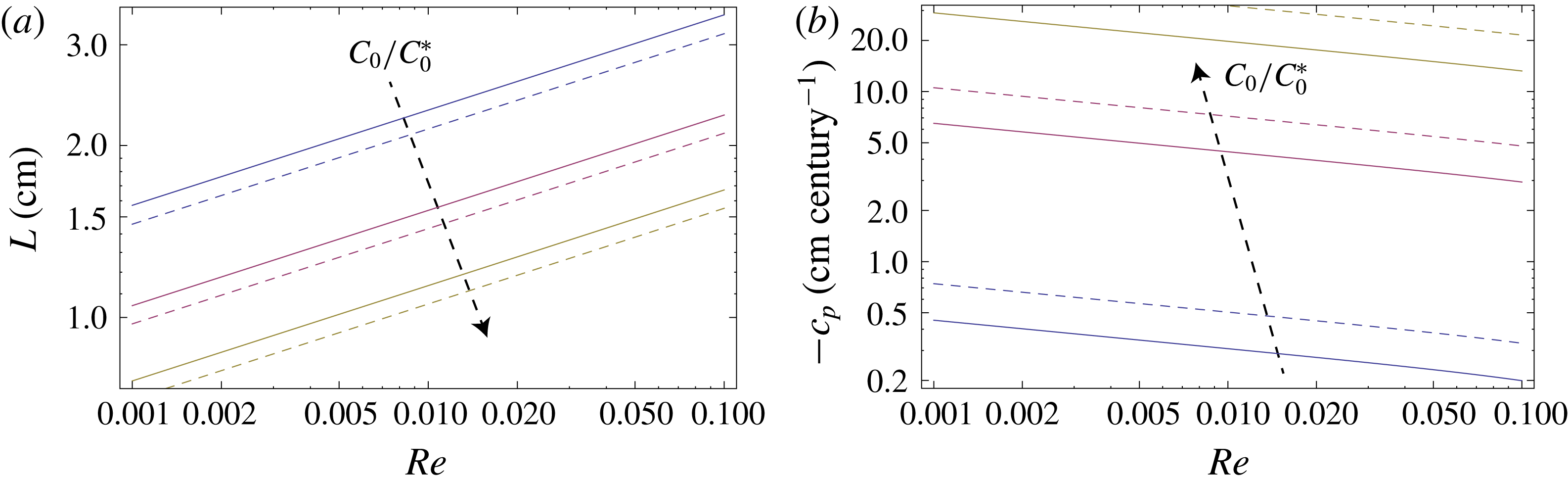
Figure 4(a) shows some values obtained from (3.9) for different degrees of supersaturations and two values of temperatures. The linear shape in the log–log chart suggests that a fair and practical approximation for
 $L$
is given by a power-law formula. In fact, by considering (3.8) and the temperature dependence of
 $p_{c}$
,
 $\unicode[STIX]{x1D708}$
and
 $\mathit{Pe}$
, we arrive at
 $$\begin{eqnarray}L\sim (0.657-0.001989T)\cdot (C_{0}/C_{0}^{\ast })^{-7/16}\mathit{Re}^{1/4}\quad [\text{m}].\end{eqnarray}$$
This formula could be used for expeditive estimations that relate patterns to hydrodynamics and geochemistry. The obtained values range from subcentimetric wavelengths for
 $\mathit{Re}=10^{-3}$
to some centimetres for
 $\mathit{Re}=10^{-2}$
.
(a) Wavelength selected in centimetres. The best fitting of the curves is given by (3.10). (b) Phase velocity corresponding to the selected wavelength. Solid lines:
 $T=288$
K; dashed lines:
 $T=293$
K. The ratio
 $C_{0}/C_{0}^{\ast }$
is set to 2, 4 and 6.

The phase velocity corresponding to the least stable mode is
 $c_{p}=-\unicode[STIX]{x1D706}_{i}(k_{m})/k_{m}$
. At verticality, its approximate relationships reads
 $$\begin{eqnarray}c_{p}(k_{m})=-1.28\cdot 10^{11}\unicode[STIX]{x1D712}{\mathcal{F}}_{0}l_{c}\left(\frac{g^{2}\mathit{Re}}{\unicode[STIX]{x1D708}}\right)^{1/3}\left(\frac{\unicode[STIX]{x1D70E}}{\mathit{Pe}}\right)^{1/2}\quad [\text{cm}~\text{century}^{-1}].\end{eqnarray}$$
As reported in figure 4(b),
 $c_{p}$
is always negative, that is the pattern migrates upstream with celerity that reaches the order of
 $10~\text{cm}~\text{century}^{-1}$
for highly supersaturated waters. These results are an agreement with the observations made by Camporeale & Ridolfi (Reference Camporeale and Ridolfi2012b
).
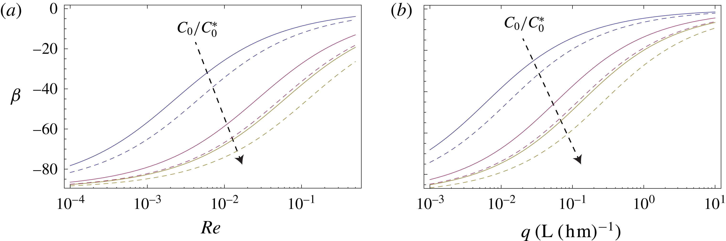
As mentioned in the Introduction, a promising paleo-reconstructive proxy is provided by the slope factor,
 $\unicode[STIX]{x1D6FD}$
, which is the angle between any constant-phase point of the wavelet and the
 $\unicode[STIX]{x1D701}$
axis (see figure 1
c,d). It is straightforward to recognize that this quantity is given by the arctangent of the ratio
 $c_{p}(k_{m})/{\mathcal{F}}_{0}$
. After some algebra, we get
 $$\begin{eqnarray}\tan \unicode[STIX]{x1D6FD}=-l_{c}\left(\frac{g}{\mathit{Re}\unicode[STIX]{x1D708}^{2}}\right)^{1/3}\sqrt{\frac{\unicode[STIX]{x1D70E}}{\mathit{Pe}}}\sim (a-bT)(C/C_{0}^{\ast })^{7/8}p_{c}^{1/3}R^{-1/2},\end{eqnarray}$$
where
 $a=0.1138$
and
 $b=0.000423$
. The values obtained with the above formula are reported in figure 5(a). In fair agreement with the numerical results obtained by Camporeale & Ridolfi (Reference Camporeale and Ridolfi2012a
), one observes that the slope factor is highly sensitive to the Reynolds number, in particular at small calcium concentrations. By recalling that the unitary water discharge is
 $q=(2/3)\unicode[STIX]{x1D708}\mathit{Re}$
, the relation (3.12) can be also given in an alternative form, by replacing
 $\mathit{Re}$
with
 $q$
(having units (
 $\text{Lh}^{-1}~\text{m}^{-1}$
)), and posing
 $a=0.0127$
and
 $b=0.00048$
. The corresponding plot is reported in figure 5(b).
The slope factor versus the Reynolds number (a) and the unitary discharge (b). Solid lines:
 $T=288$
K; dashed lines:
 $T=293$
K. The ratio
 $C_{0}/C_{0}^{\ast }$
is set to 2, 4 and 6.

Furthermore, a straightforward analysis of the convective-absolute nature of the instability is also achievable. By definition, a system is convectively unstable if the response to an impulsive perturbation increases in time but migrates and decays to zero at all the spatial locations, and it is absolutely unstable if the response grows exponentially in time at all spatial locations (Schmid & Henningson Reference Schmid and Henningson2001). If
 $k^{\ast }$
is the wavenumber that corresponds to the solution of the saddle point condition
 $\unicode[STIX]{x2202}\unicode[STIX]{x1D706}/\unicode[STIX]{x2202}k=0$
, provided the causality principle is satisfied, it follows that the instability is convective if
 $\unicode[STIX]{x1D706}_{r}[k_{m}]>0$
and
 $\unicode[STIX]{x1D706}_{r}[k^{\ast }]<0$
and it is absolute if
 $\unicode[STIX]{x1D706}_{r}[k_{m}]>0$
and
 $\unicode[STIX]{x1D706}_{r}[k^{\ast }]>0$
(the so-called Briggs’ criterion). In the present case, and under the same approximations made to obtain (3.9), the saddle point condition provides the following three solutions:
 $$\begin{eqnarray}\displaystyle & \displaystyle k_{1}^{\ast }=\frac{2\text{i}\mathit{Re}^{2/9}}{135\,15^{2/3}}\left(\frac{405\sqrt[3]{5}}{K^{1/3}}+270\sqrt[3]{3}\frac{\mathit{Pe}\,\mathit{Re}^{2/9}}{{\mathcal{F}}_{0}K^{2/3}}-24\sqrt[3]{5}\frac{\mathit{Pe}^{3}K^{1/3}\mathit{Re}^{2/3}}{{\mathcal{F}}_{0}^{3}K^{4/3}}+16\sqrt[3]{3}\frac{\mathit{Pe}^{4}R^{8/9}}{{\mathcal{F}}_{0}^{4}K^{5/3}}\right), & \displaystyle \nonumber\\ \displaystyle & & \displaystyle\end{eqnarray}$$
 $$\begin{eqnarray}\displaystyle \displaystyle k_{2}^{\ast } & = & \displaystyle \frac{2\mathit{Re}^{2/9}\sqrt[6]{-1}}{135\,15^{2/3}}\left(\frac{16\sqrt[3]{3}\mathit{Pe}^{4}\mathit{Re}^{8/9}}{{\mathcal{F}}_{0}^{4}K^{5/3}}-\frac{24\sqrt[3]{5}\mathit{Pe}^{3}(-\mathit{Re})^{2/3}}{{\mathcal{F}}_{0}^{3}K^{4/3}}\right.\nonumber\\ \displaystyle & & \displaystyle +\left.\frac{270\sqrt[3]{3}\mathit{Pe}\,\mathit{Re}^{2/9}}{{\mathcal{F}}_{0}K^{2/3}}+\frac{405(-1)^{2/3}\sqrt[3]{5}}{\sqrt[3]{K}}\right),\end{eqnarray}$$
 $$\begin{eqnarray}\displaystyle & \text{Re}[k_{3}^{\ast }]=-\text{Re}[k_{2}^{\ast }],\quad \text{Im}[k_{3}^{\ast }]=\text{Im}[k_{2}^{\ast }]. & \displaystyle\end{eqnarray}$$
The above wavenumbers correspond to three values of the absolute growth rate, i.e.
 $\unicode[STIX]{x1D706}_{i}^{\ast }=\unicode[STIX]{x1D706}_{r}(k_{i}^{\ast })$
. By numerical inspection, it can be shown that the larger absolute growth rate is always negative. It follows that, at verticality (
 $\unicode[STIX]{x1D703}_{1}=0$
), the instability turns out invariably convective. This result is in agreement with a more refined analysis made on the 2-D model by Vesipa et al. (Reference Vesipa, Camporeale and Ridolfi2015), which used the cusp method to determine the convective-absolute nature of a Orr–Sommerfeld-like model.
4 Discussion and conclusions
In the present analysis, a gradient expansion technique applied to the Navier–Stokes equations, the diffusion–advection equation and an evolution equation for the shape of the liquid–solid interface, has allowed a closed form of the dispersion relation for the crenulation formation to be obtained in a fully analytical way (3.4). Other important outcomes of this procedure are: (i) the computation of the lower and upper bound of unstable wavenumbers (3.7); (ii) the evaluation of the selected wavelength of crenulations (3.9); (iii) the computation of phase velocity (3.11); (iv) the evaluation of the slope factor (3.12) and (v) the analytical investigation of the convective-absolute nature of the instability. The analytical treatment of the theory has allowed us to identify a single parameter (
 $\unicode[STIX]{x1D70E}$
) that contains all the relevant geochemical information and that, by exploiting the geochemical relationship reported in appendix A, has been expressed in terms of a simple function of the ratio
 $C_{0}/C_{0}^{\ast }$
(where
 $C_{0}$
is the calcium concentration and
 $C_{0}^{\ast }$
is its saturation value) and the atmospheric carbon dioxide partial pressure (see (3.8)).
The validity domain of the gradient expansion technique used herein has been discussed in detail by Kalliadasis et al. (Reference Kalliadasis, Ruyer-Quil, Scheid and Velarde2012) through a comparison with the temporal hydrodynamic modes provided by the numerical solution of the Orr–Sommerfeld equation. The gradient expansion was recognized to be ‘exact close to criticality as far as critical, neutral conditions and interfacial quantities are concerned’ (Kalliadasis et al.
Reference Kalliadasis, Ruyer-Quil, Scheid and Velarde2012). This means that, in order to assure convergence of the theory, the criterion was recognized to be
 $\mathit{Re}-\mathit{Re}_{c}<1$
, where
 $\mathit{Re}_{c}$
is the critical Reynolds number for the hydrodynamic instability. In the present morphodynamic analysis, the quasi-steady approximation precludes consideration of the hydrodynamic modes, but considers just the morphological mode. However, recalling that close to verticality the critical condition to the trigger of the surface waves is
 $\mathit{Re}_{c}\sim 0$
, the same criterion suggests keeping
 $\mathit{Re}$
smaller than unity. For this reason, all the computations were shown in the conservative range
 $10^{-3}<\mathit{Re}<10^{-1}$
, which is quite representative of most of the caves’ conditions.
The selected wavelength has been interpolated by a power-law formula, wherein the
 $\mathit{Re}^{1/4}$
dependence confirms the previous numerical theories of Camporeale & Ridolfi (Reference Camporeale and Ridolfi2012a
) and Vesipa et al. (Reference Vesipa, Camporeale and Ridolfi2015). Furthermore, the interval range of the values obtained for
 $L$
(figure 4
a) is coherent with the latter paper, where a correction of a boundary condition allowed also centimetric wavelengths (while in the former paper the results were erroneously confined to subcentimetric patterns only). A
 $\mathit{Re}$
-dependence in the geometric features of the patterns is an advantage when looking for new paleo-climatic proxies, which are required to be highly sensitive in the prediction of
 $L$
when
 $\mathit{Re}$
or
 $C_{0}$
change over time. This fact is even more decisive in the plot of the phase velocity, which, at verticality, shows upstream migration of the patterns, with a change in
 $c_{p}$
of several orders of magnitude when the ratio
 $C_{0}/C_{0}^{\ast }$
varies from 2 to 6 (figure 4
b). Therefore, an easy-to-use formula has also been derived for the slope factor
 $\unicode[STIX]{x1D6FD}$
(3.12), in terms of a power-law function of
 $T$
,
 $C_{0}/C_{0}^{\ast }$
and
 $p_{c}$
. This latter formula provides a promising tool for paleo-flow reconstruction since it is quite sensitive to the flow conditions. In order to give an idea of the accuracy of the method, it is sufficient to solve (3.12) with respect to
 $q$
and then to derive in
 $\unicode[STIX]{x1D6FD}$
. It turns out that
 $|\text{d}q/q|\,=\,\unicode[STIX]{x1D6FE}(\unicode[STIX]{x1D6FD})|\text{d}\unicode[STIX]{x1D6FD}/\unicode[STIX]{x1D6FD}|$
, with
 $\unicode[STIX]{x1D6FE}\,\sim \,0.07\unicode[STIX]{x1D6FD}\csc [0.035\unicode[STIX]{x1D6FD}]$
. In the range
 $\unicode[STIX]{x1D6FD}=10^{\circ }{-}80^{\circ }$
,
 $\unicode[STIX]{x1D6FE}$
varies in the range 2–15. For example, a variation
 $\text{d}\unicode[STIX]{x1D6FD}=\pm 10^{\circ }$
around
 $\unicode[STIX]{x1D6FD}=45^{\circ }$
implies a relative change in the discharge of
 $\pm 62\,\%$
.
Finally, it should be also mentioned that the present technique could be a promising tool in other morphodynamic contexts, where a falling film interacts dynamically with a substrate. For instance, the case of pattern formation over icicles provides very similar dynamics and patterns (see figure 1) and still awaits a fully analytical treatment that excludes numerical or approximate solutions of the Orr–Sommerfeld problem (e.g. Ueno et al. Reference Ueno, Farzaneh, Yamaguchi and Tsuji2010). Likewise, ripple or dune formation over sediments under laminar flows could be another interesting application.
Appendix A. The geochemical factors of (2.45)
An exact expression of terms
 $\unicode[STIX]{x1D6E4}$
and
 $\unicode[STIX]{x1D705}$
has been derived by adopting the procedure reported by Short et al. (Reference Short, Baygents and Goldstein2005b
) – see (50)–(52) therein – and also considering the effect of the activity coefficients. Furthermore, following Camporeale & Ridolfi (Reference Camporeale and Ridolfi2012a
), the concentration of [
 $H^{+}$
] (or equivalently the pH) has been eliminated by using the electroneutrality condition, the ionic product of water, the solubility product of calcite and two non-rate-limited reactions involving the concentrations of carbonates. The final result is
 $$\begin{eqnarray}\displaystyle & \displaystyle \unicode[STIX]{x1D6E4}=\frac{2C_{0}^{2}\tilde{D}_{0}^{2}\unicode[STIX]{x1D6FE}_{2}\unicode[STIX]{x1D6FE}_{1}\left({\displaystyle \frac{2C_{0}^{2}\unicode[STIX]{x1D6FE}_{2}\unicode[STIX]{x1D6FE}_{1}k_{1}^{-}-K_{2}}{\unicode[STIX]{x1D6FE}_{3}K_{c}}}+k_{1}^{-}\right)}{{\mathcal{D}}(C_{0}^{2}\unicode[STIX]{x1D6FE}_{2}\unicode[STIX]{x1D6FE}_{1}+\unicode[STIX]{x1D6FE}_{3}K_{c})}, & \displaystyle\end{eqnarray}$$
 $$\begin{eqnarray}\displaystyle & \displaystyle \unicode[STIX]{x1D705}=\frac{\unicode[STIX]{x1D6FE}_{3}K_{c}K_{w}}{4C_{0}^{3}\unicode[STIX]{x1D6FE}_{2}\unicode[STIX]{x1D6FE}_{1}K_{2}}-\frac{C_{0}\unicode[STIX]{x1D6FE}_{2}\unicode[STIX]{x1D6FE}_{1}K_{2}}{\unicode[STIX]{x1D6FE}_{3}K_{c}}+\frac{\unicode[STIX]{x1D6FE}_{3}K_{c}K_{H}p_{c}(C_{0}^{2}\unicode[STIX]{x1D6FE}_{3}\unicode[STIX]{x1D6FE}_{1}+\unicode[STIX]{x1D6FE}_{3}K_{c})(2C_{0}^{2}\unicode[STIX]{x1D6FE}_{3}\unicode[STIX]{x1D6FE}_{1}\unicode[STIX]{x1D6FE}_{4}k_{1}^{+}K_{2}+k_{2}^{+}K_{w})}{4C_{0}^{5}\unicode[STIX]{x1D6FE}_{2}\unicode[STIX]{x1D6FE}_{1}\unicode[STIX]{x1D6FE}_{4}K_{2}(2C_{0}^{2}\unicode[STIX]{x1D6FE}_{2}\unicode[STIX]{x1D6FE}_{1}k_{1}^{-}K_{2}+\unicode[STIX]{x1D6FE}_{3}k_{2}^{-}K_{c})}, & \displaystyle \nonumber\\ \displaystyle & & \displaystyle\end{eqnarray}$$
where
 $\{\unicode[STIX]{x1D6FE}_{1},\unicode[STIX]{x1D6FE}_{2},\unicode[STIX]{x1D6FE}_{3},\unicode[STIX]{x1D6FE}_{4}\}$
are the activity coefficients, computed by the extended Debye–Hückel theory for the chemical species
 $\{\text{HCO}_{3}^{-},\text{Ca},\text{H}^{+},\text{OH}^{-}\}$
, respectively,
 $p_{c}$
is the carbon dioxide partial pressure in the air and
 ${\mathcal{D}}$
is the calcium diffusivity coefficient in water. The terms
 $K_{i}$
and
 $k_{1,2}^{\pm }$
are reaction constants of the chemical model, which can be found in Kaufmann & Dreybrodt (Reference Kaufmann and Dreybrodt2007) or in the Additional Material of Vesipa et al. (Reference Vesipa, Camporeale and Ridolfi2015). We finally emphasize that the use of the above formulas can be bypassed by adopting the expression
 $$\begin{eqnarray}\unicode[STIX]{x1D70E}=10^{-4}(C_{0}/C_{0}^{\ast })^{7/4}p_{c}^{2/3}(\mathit{Re}\csc \unicode[STIX]{x1D703})^{2/3},\end{eqnarray}$$
as reported in the text, which derives from an interpolation of an extensive use of (A 1) and (A 2) and provides
 $\unicode[STIX]{x1D70E}$
, namely the only term that is needed for the present theory to characterize the geochemical conditions.