2 Experimental set-up, flow organisation and measurement methods

The experiment was carried out in the hypo-turbulent supersonic wind tunnel at IUSTI. It is a continuous facility with a closed-loop circuit. It can be run for 4 h in well-controlled operating conditions. For this experiment, it is operated at a nominal Mach number of 2.3. A control system stabilises the stagnation pressure to a prescribed setting. Typically, when the stagnation pressure in the external flow is $0.5\times 10^{5}~\text{N}~\text{m}^{-2}$ , its variations in time are less than $\pm 0.2\,\%$ . The stagnation temperature is typically atmospheric, with a drift less than $1~\text{K}~\text{h}^{-1}$ . The level of background turbulence in the outer flow is essentially due to aerodynamic noise radiated by the boundary layers. Its level is less than $0.1\,\%$ for the turbulence intensity of velocity.

The 2D supersonic equilibrium turbulent boundary layer under investigation develops on the nozzle floor, which is a flat plate. The incoming conditions (inlet conditions for the interaction) are located at a distance larger than 25 cm downstream of the contoured part of the nozzle block (more than 25 boundary layer thicknesses). The test section has a size of $\text{height}\times \text{span}=122.1~\text{mm}\times 170~\text{mm}$ at $x_{w}=180~\text{mm}$ (origin $x_{w}=0$ at the end of the contoured part of the nozzle). The coordinates $x_{w}$ and $y_{w}$ are taken in a reference system related to the wind tunnel, $x_{w}$ being the longitudinal coordinate along the wall, and $y_{w}$ the normal coordinate perpendicular to it. The span of $170~\text{mm}$ is constant in the whole flow. The layer is subjected to a shock wave produced by a generator placed in the external flow. The shock generator is a sharp-edged plate fixed on the ceiling of the wind tunnel. Its leading edge is located in the potential flow. It spans the entire test section and generates an oblique shock wave impinging on the floor boundary layer. Its angle with respect to the potential flow $\unicode[STIX]{x1D703}$ is set at $8^{\circ }$ and $9.5^{\circ }$ , for the two cases under consideration. The geometrical details of the flow conditions and of the configurations, including the CAO files for the nozzle contours, are given in Doerffer et al. (Reference Doerffer, Hirsch, Dussauge, Babinsky and Barakos2009), and in the ERCOFTAC QNET-CFD knowledge database produced by Dussauge et al. (Reference Dussauge, Dupont, Sandham and Garnier2013). As reported in Doerffer et al. (Reference Doerffer, Hirsch, Dussauge, Babinsky and Barakos2009), the vertical distance from the wall at which the leading edge of the shock generator is placed is $104.7~\text{mm}$ for the $8^{\circ }$ interaction, and $107.6~\text{mm}$ in the $9.5^{\circ }$ case. This corresponds to an aspect ratio span/height of $1.62$ for the $8^{\circ }$ deviation and of 1.58 for the $9.5^{\circ }$ interaction.

The incoming boundary layer is turbulent and fully developed. As reported in Doerffer et al. (Reference Doerffer, Hirsch, Dussauge, Babinsky and Barakos2009) and Piponniau et al. (Reference Piponniau, Dussauge, Debiève and Dupont2009), upstream of the interaction, the thicknesses of the boundary layer, displacement and momentum are, respectively, $11~\text{mm}$ , $3.4~\text{mm}$ and $0.96~\text{mm}$ . The Reynolds number based on momentum thickness is $5100$ . The longitudinal coordinate $x_{w}$ of the mean location of the reflected shock at the wall is denoted $X_{0}$ . The length of interaction $L$ is defined as the distance between $X_{0}$ and the extrapolation to the wall of the incident shock; it is used to normalise the longitudinal coordinate $x_{w}$ . The dimensionless coordinate is therefore $X^{\ast }=(x_{w}-X_{0})/L$ , and the interaction extends mainly from $X^{\ast }=0$ to $1$ . The interaction length is $41~\text{mm}$ for a flow deflection angle of $8^{\circ }$ and $71~\text{mm}$ for the $9.5^{\circ }$ case.

Figure 1.

Spark schlieren visualisation of the interaction, for a deflection angle of $9.5^{\circ }$ . Superimposed onto the schlieren visualisation is the standard deviation of the vertical velocity component in the frame of reference of the wind tunnel, obtained by particle image velocimetry (PIV) measurements (grey scale associated, $(\text{m}~\text{s}^{-1})$ ).

The global organisation of the incident shock wave–boundary layer interaction illustrated by spark schlieren visualisation and by particle image velocimetry (PIV) measurements is presented in figure 1, in which the flow deviation due to the incident shock is $9.5^{\circ }$ , and the pressure gradient is strong enough for the layer to separate. Measurements of the velocity fields along the interaction have been made in vertical planes, along the centreline of the test section.

The spatial resolution of the PIV measurements was $50~\text{pixel}~\text{mm}^{-1}$ , leading to a longitudinal field of view (FOV) of $32~\text{mm}$ . Such a reduced field of view was necessary to correctly measure the turbulent quantities along the interaction: indeed, we had to measure vertical components that can be 10 times lower than the mean longitudinal velocity.

Particle image velocimetry (PIV) measurements were performed with a Dantec Dynamics system. The light sheets were generated by a double-pulse Nd:Yag laser (New Wave Solo II), which delivered 30 mJ per pulse (flashing time $5~\text{ns}$ ), two consecutive flashes being separated by $1~\unicode[STIX]{x03BC}\text{s}$ . The images of particles were recorded by FlowSense cameras ( $1600~\text{pixels}\times 1200~\text{pixels}$ ). Explorations were made in vertical planes, along the longitudinal axis of the wind tunnel, to get the velocity fields along the interaction. As the shock generator was fixed on the ceiling, some optical arrangements were necessary to illuminate the test section: a prism was placed in the diffuser to allow the laser sheet to propagate backwards to the measurement area. Sets of $4000$ digital images were used. Two cameras were lined up next to each other in the longitudinal direction to provide a wide field of view. The two pictures recorded by each camera were overlapped by approximately 10 %. A calibration grid was recorded, and the spatial correlation function between pictures gave spatial correspondences between both fields; a global panoramic picture was then created, covering an area of approximately $160~\text{mm}\times 20~\text{mm}$ ( ${\approx}16\unicode[STIX]{x1D6FF}_{0}\times 2\unicode[STIX]{x1D6FF}_{0}$ ).

Incense smoke was used as seeding particles. After sedimentation of the smoke, the particles were injected from the wall, upstream of the sonic section on the wind tunnel axis. As the wind tunnel stagnation pressure was less than atmospheric pressure, the particles were naturally entrained into the flow. The time constant of the particles was estimated by using PIV measurements of the mean velocity across the incident reflected shock outside the boundary layer. A time constant of $4.55~\unicode[STIX]{x03BC}\text{s}$ was derived corresponding to diameters of $0.5~\unicode[STIX]{x03BC}\text{m}$ (see Elena, Tedeschi & Gouin Reference Elena, Tedeschi and Gouin1999). Samimy & Lele (Reference Samimy and Lele1991) suggest that the particles accurately followed the velocity fluctuations in a turbulent mixing layer if the Stokes number $St=\unicode[STIX]{x1D70F}_{p}/\unicode[STIX]{x1D70F}_{f}$ (with $\unicode[STIX]{x1D70F}_{f}=\unicode[STIX]{x1D6FF}/U_{\infty }$ and $\unicode[STIX]{x1D70F}_{p}$ the time response of the particles) was less than $0.5$ . In the present experiments, the Stokes number was 0.23. This low value showed that the particles were able to follow the large-scale velocity fluctuations in the interaction and particularly in the separation and in the shear layer: the seeding was well adapted to this study for capturing the energetic fluctuations.

For the wide FOV measurements, the calibration factor of the pictures was $17~\text{pixels}~\text{mm}^{-1}$ . The intercorrelation was carried out recursively from a cell of size $128\times 64$ to a final cell size of 64 pixels horizontally by 32 pixels vertically with a Gaussian weighting window applied to the interrogation cell. Therefore, the final effective cell size was $32~\text{pixels}\times 16~\text{pixels}$ ; this led to a PIV resolution of $0.64~\text{mm}\times 0.32~\text{mm}$ . An overlap of 50 % between cells provided a final field of $138\times 505$ vectors, after assembly of the different acquisitions.

The subpixel interpolation is assumed to have an accuracy of 0.1 pixel. This accuracy, combined with the spatial resolution and the time between the two flashes, gives a resolution of $2~\text{m}~\text{s}^{-1}$ on the velocity. As samples of 4000 images were used for root-mean-square (r.m.s.) values of velocity typically of $0.1Ue$ ( $Ue$ is the external velocity), the evaluation of statistical uncertainty, given the limited size of the sample, is $0.0016Ue$ , i.e. typically $0.8~\text{m}~\text{s}^{-1}$ , if $Ue\approx 500~\text{m}~\text{s}^{-1}$ . Finally, the influence of the presence of fluctuations in the third direction $w^{\prime }$ was estimated from the work of Scharnowski et al. (Reference Scharnowski, Grayson, de Silva, Hutchins, Marusic and Kähler2017). The thickness of the light sheet is approximately $1~\text{mm}$ . For a velocity fluctuation $w^{\prime }$ in the spanwise direction of $0.1Ue$ (with $Ue\approx 500~\text{m}~\text{s}^{-1}$ ) and a time delay of $1~\unicode[STIX]{x03BC}\text{s}$ , the displacement is $5\times 10^{-5}~\text{m}$ , while the displacement/thickness ratio is close to $5\times 10^{-2}$ , so that the loss of correlation due to such three-dimensional (3D) perturbations is probably significantly smaller than the other possible sources of uncertainty.

Figure 2.

Impact of the spatial resolution of the PIV measurements on the accuracy of the Reynolds stresses: ♢, laser Doppler anemometry (LDA) measurements; ○, large field-of-view (FOV) (PIV); ▫, intermediate FOV PIV; ♦, reduced FOV PIV.

Figure 3.

Comparison LDA versus PIV velocity measurements in the upstream boundary layer. Closed symbols, PIV (reduced FOV); open symbols, LDA. (a) Mean velocity in Van Driest representation. (b) Longitudinal (○) and normal (▵) r.m.s. velocity in Morkovin representation (▪, Humble et al. (Reference Humble, Elsinga, Scarano and Van Oudheusden2009a )). (c) Reynolds shear stress in Morkovin representation. Black lines, Klebanoff’s data ( $M=0$ , Klebanoff (Reference Klebanoff1954)).

A global control of the accuracy was performed by checking the influence of spatial resolution resulting from the field of view. Figure 2 shows the Reynolds shear stress measurements for different PIV spatial resolution, taking laser Doppler anemometry (LDA) measurements as a reference, inside the incoming boundary layer with the same seeding as the PIV. Details of the LDA system will be given below. Three different fields of view are presented: $16~\text{pixels}~\text{mm}^{-1}$ (large FOV PIV), $32~\text{pixels}~\text{mm}^{-1}$ (intermediate FOV PIV) and $50~\text{pixels}~\text{mm}^{-1}$ (reduced FOV PIV). Very clearly, the reduced FOV measurements agree with the LDA determination, and increasing the spatial resolution of the PIV measurements gives a better description of the turbulent quantities. This is also exemplified by comparison with the Klebanoff profiles (see figure 3) where the measured boundary layer profiles in Morkovin’s representation are in agreement with the subsonic profiles (Klebanoff Reference Klebanoff1954), down to $y_{w}/\unicode[STIX]{x1D6FF}=0.1$ . Examining the discrepancy between PIV and LDA results suggests that the accuracy of the PIV measurements on the Reynolds stresses is $\pm 5\,\%$ . This is for measurements in the frame of reference related to the flat plate. In our analysis, a frame of reference related to the shear layer is used. As will be explained in the next section, orientation of the longitudinal axis is determined empirically. A conservative estimate of the uncertainty on this angle is $0.5^{\circ }$ . This is at the origin of an uncertainty on Reynolds stresses, estimated in the centre of the layer, between 0.5 % (on $\overline{u^{\prime \,2}}$ ) and 3 % (on $\overline{u^{\prime }v^{\prime }}$ ). The value of 3 % is retained as a conservative estimate for all stresses, so that the final assessment of the total uncertainty on the Reynolds stress is $\pm 8\,\%$ .

The measurements represent effectively the average over the size of the interrogation window. An assessment of this space integration can be made as follows. The method implicitly assumes that, for all scales, particles are convected at the local flow velocity. In inhomogeneous conditions, a problem can arise if the velocity fluctuation is affected by the finite size of the interrogation cell. A criterion was proposed by Dussauge & Dupont (Reference Dussauge and Dupont2005), who assumed that a cell is sufficiently small if the velocity variation $\unicode[STIX]{x0394}U$ over the cell is small compared to the velocity fluctuation, i.e.  $\unicode[STIX]{x0394}U\ll u^{\prime }$ . For a cell of height $h$ , the previous condition, after linearisation, leads to

(2.1a,b ) $$\begin{eqnarray}h\frac{\unicode[STIX]{x2202}U}{\unicode[STIX]{x2202}y}\ll u^{\prime }\quad \text{or}\quad h\ll \frac{u^{\prime }}{\unicode[STIX]{x2202}U/\unicode[STIX]{x2202}y}.\end{eqnarray}$$

On the right-hand side we recognise the definition of the mixing length. In the external boundary layer the mixing length is constant, $l\simeq 0.1\unicode[STIX]{x1D6FF}$ . Therefore, in the external layer, it is possible to derive the simple criterion $h\ll 0.1\unicode[STIX]{x1D6FF}$ which gives an indication of an acceptable size for the interrogation window. In the present experiment, in the incoming boundary layer, $h/\unicode[STIX]{x1D6FF}=0.06$ . This is not much less than 0.1, but this seems to be an adequate choice, as will be shown in the next section, by cross-checking PIV measurements with laser Doppler determinations.

In order to have reference data for validating PIV results, LDA measurements have also been carried out with a two-component system operated in forward scatter mode. The probe volume was an ellipsoid of $0.2~\text{mm}\times 0.2~\text{mm}\times 1~\text{mm}$ , taking into account the off-axis setting of the receiving optics. The same seeding as in PIV measurements was used, with a 7 W argon laser and an optical fibre between the laser source and the optical head. Photomultiplier signals are low-passed at 50 MHz and recorded with an eight-bit digitiser (model Acqiris DP235) with 2M words inboard memory, at a sampling rate of 100 MHz. LDA signals are then processed with a home-made algorithm. For each point of measurement, around $4\times 10^{3}$ points were recorded.

The quality of the flow in particular was examined in the past. Such interactions may develop a 3D structure because of the interactions produced by the shock generator with the sidewalls, which may alter deeply the structure of the separated zone (see Babinsky, Oorebeek & Cottingham Reference Babinsky, Oorebeek and Cottingham2013; Eagle & Driscoll Reference Eagle and Driscoll2014; Wang et al. Reference Wang, Sandham, Hu and Liu2015, among others). Spanwise wall pressure distributions were measured and PIV measurements in planes parallel to the wall were performed. The results were published in Dupont et al. (Reference Dupont, Haddad, Ardissone and Debiève2005), Dussauge, Dupont & Debiève (Reference Dussauge, Dupont and Debiève2006) and Dussauge & Piponniau (Reference Dussauge and Piponniau2008); and they were reported by Garnier in Doerffer et al. (Reference Doerffer, Hirsch, Dussauge, Babinsky and Barakos2009) and Garnier (Reference Garnier2009). The results have shown that, in the $8^{\circ }$ interaction and upstream of reattachment, no significant three-dimensionality developed over more than half of the span. In the $9.5^{\circ }$ interactions, conical interactions are formed along the sidewalls. The reattachment zone is clearly 3D, but, in the part where the mixing layer takes place and in qualitative agreement with the results of Wang et al. (Reference Wang, Sandham, Hu and Liu2015), the flow along the centre of the wind tunnel remains 2D over a significant spanwise distance (approximately half of the span), so that the usual 2D analysis can still be used.

3 Upstream boundary layer

The incoming boundary layer has already been partly described in some previous papers (e.g. Piponniau et al. Reference Piponniau, Dussauge, Debiève and Dupont2009). However, a detailed description of the velocity field and the Reynolds stresses was needed, in particular to obtain an assessment of the measurement accuracy.

They are described in the reference section $x_{w}=240~\text{mm}$ located $3\unicode[STIX]{x1D6FF}_{0}$ upstream of the interaction. The results are given in figure 3. Figure 3(a) presents the comparison of the Van Driest transformed velocity profiles $V_{vd}$ given by PIV and by LDA. As in Piponniau et al. (Reference Piponniau, Dussauge, Debiève and Dupont2009), density was determined from a Walz/modified Crocco relation, with a recovery factor of $0.89$ . It can be seen that the agreement is very good, except for the first point at $y_{w}^{+}\approx 20$ , corresponding to a distance of ${\approx}0.28~\text{mm}$ from the wall, where bias and uncertainties exist probably for both methods. The solid line corresponds to the classical log law,

(3.1) $$\begin{eqnarray}\frac{V_{vd}}{u_{\unicode[STIX]{x1D70F}}}=\frac{1}{\unicode[STIX]{x1D705}}\ln (y_{w}^{+})+B,\end{eqnarray}$$

with $\unicode[STIX]{x1D705}=0.41$ and $B=5.25$ . The value of $u_{\unicode[STIX]{x1D70F}}$ was determined from the slope of the log zone.

The excellent agreement between two independent methods suggests that we can confidently accept the accuracy of these measurements. Figure 3(b) presents the longitudinal and vertical r.m.s. velocity in Morkovin’s representation. Again, the agreement between LDA and PIV is more than satisfactory. Data from other work at a Mach number of $2.1$ (Humble et al. Reference Humble, Elsinga, Scarano and Van Oudheusden2009a ) have also been plotted for comparison. Moreover, considering the expected accuracy of the present Reynolds stress measurements, the agreement with Klebanoff’s subsonic data (Klebanoff Reference Klebanoff1954) is also very good. This provides a well-controlled verification of Morkovin’s hypothesis at Mach numbers around 2.

The question of the shear stress $\overline{-u^{\prime }v^{\prime }}$ is more difficult. The previous section has shown that accuracy can be an issue for this quantity. It can be seen (figure 3 c) that the overall agreement of PIV, LDA and Klebanoff is good for $y/\unicode[STIX]{x1D6FF}_{0}>0.1$ .

4 Analysis of velocity profiles

Velocity was measured in two cases of interactions at a Mach number of 2.3. The corresponding isovelocity maps are presented in figure 4. The maps of mean velocity, r.m.s. velocity (longitudinal and wall-normal components) and turbulent shear stresses are presented. It appears that, in both cases, the levels of velocity fluctuations are dramatically increased in the interactions and this high level persists over a long distance downstream of the interaction. As suggested by several authors (Na & Moin Reference Na and Moin1998; Dupont et al. Reference Dupont, Haddad and Debiève2006, Reference Dupont, Piponniau, Sidorenko and Debiève2008; Humble, Scarano & Van Oudheusden Reference Humble, Scarano and Van Oudheusden2009b ), the flow at the edge of the separated zone looks like a mixing layer. This led us to analyse the velocity and Reynolds stress profiles in a particular frame of reference related to this mixing layer. In figure 5, the map of $\sqrt{\overline{u^{\prime \,2}}}$ is shown in the frame of reference related to the wall, again evidencing the zone of high fluctuation level, which grows linearly in space. This is illustrated by the two oblique lines which give a first hint of the zone where the mixing layer is formed. This drawing was not used to define the boundaries of the layer. However, only the bisector was determined as a first guess in an iterative process for defining the longitudinal axis. Defining this axis is constrained by the fact that, along $Ox_{w}$ , after rotation of the frame of reference, the mean longitudinal velocity should be constant, the transverse mean velocity should be close to zero, and the Reynolds stresses should be constant. A procedure of trial and error was used to change the slope and the location $x_{0}$ of the intersection of the axis with the wall. The final result is shown in figures 6(a) for $U$ and $V$ and 6(b) for the Reynolds stresses. It can be seen that $U$ and $V$ are reasonably constant along $Ox$ , and that $V$ is close to zero. The Reynolds stresses are also approximately constant. The rotation of the axis is $11^{\circ }$ (respectively $9^{\circ }$ ) for the $9.5^{\circ }$ interaction (respectively $8^{\circ }$ interaction). If the origin is chosen at the foot of the reflected mean shock, the resulting values of the intersection of this axis with the wall are $x_{0}=-2~\text{mm}$ and $-4~\text{mm}$ ( $x_{0}/\unicode[STIX]{x1D6FF}=-0.18$ and $-0.36$ ) for the $9.5^{\circ }$ interaction and $8^{\circ }$ interaction, respectively, i.e. close to the foot of the shock.

Figure 4.

The $8^{\circ }$ (a) and $9.5^{\circ }$ (b) iso-values for (from top to bottom): mean longitudinal velocity; mean normal velocity; longitudinal r.m.s. velocity; normal r.m.s. velocity; and turbulent shear stress.

Figure 5.

R.m.s. longitudinal velocity in the wind tunnel coordinate system, $\unicode[STIX]{x1D703}=9.5^{\circ }$ . Black lines delimit the mixing layer and were used for a first estimate of its virtual origin.

The angles are close to the value of $10^{\circ }$ reported by Délery & Marvin (Reference Délery and Marvin1986) for the flow deviation at Mach number 2.5 downstream of the separation shock. In the rest of the text, the system of reference is related to the mixing layer. It is denoted $Ox,Oy$ . Moreover, we use the same notation for velocity components $U,V,u^{\prime }v^{\prime }$ defined now in the system of coordinates related to the mixing layer.

Figure 6.

Evolution along the estimated centreline of the mean longitudinal and vertical velocity (a) and of the Reynolds stresses (b) in the mixing layer coordinate system and for $\unicode[STIX]{x1D703}=9.5^{\circ }$ .

The results on the mean velocity and on the Reynolds stresses are shown in figure 7 for the $8^{\circ }$ and $9.5^{\circ }$ cases, in the representation $U/Ue$ versus $y/(x-x_{0})$ . Here $Ue$ is the velocity on the high-speed side, downstream of the reflected shock; $Ue=500~\text{m}~\text{s}^{-1}$ for the $8^{\circ }$ deviation and $490~\text{m}~\text{s}^{-1}$ for the $9.5^{\circ }$ interaction. Reynolds stresses are normalised by  $Ue^{2}$ .

In the $9.5^{\circ }$ interaction, the mean velocity profiles (figure 7 b) collapse for $y/(x-x_{0})<0.1$ . In the same range, there is also a good collapse of the Reynolds stress profiles (figure 7 c,e,g); their shape looks like their canonical mixing layer counterparts. For larger values, the velocity is not distributed along a single curve, and self-similarity is not found. The same properties are observed in the $8^{\circ }$ interaction (figure 7), however with a larger scatter.

Figure 7.

Velocity profiles in the mixing layer coordinate system, $\unicode[STIX]{x1D703}=8^{\circ }$ (a,c,e,g) and $\unicode[STIX]{x1D703}=9.5^{\circ }$ (b,d,f,h). (a,b) Black dots, mean longitudinal velocity normalised by $Ue$ ; grey line, $V/Ue$ ; dashed line, $V/Ue$ determined from conservation. (c,d) Variance of the longitudinal velocity. (e,f) Variance of the normal velocity. (g,h) Turbulent shear stress. All stresses normalised by $Ue^{2}$ .

The influence of the reference system can be illustrated by comparing the same profiles in the system of coordinates related to the flat plate (figure 8). As the velocity components are not invariant in a rotation, the picture is quite different, no trend to similarity is observed, and a large scatter appears on all quantities. In particular, the shear stress has scattered values and the correlation coefficient (not shown) is far from the expected distribution in shear flows. This underlines the importance of such a choice for the physical analysis of the flow.

Coming back to figure 7, self-similarity has been found on the mean velocity and on the Reynolds stresses for $y/(x-x_{0})<0,1$ . If there is a collapse of the profiles when plotted versus $y/(x-x_{0})$ , the locus of iso-values is on lines $y/(x-x_{0})=\text{const.}$ , i.e. straight lines. Therefore, this part of the flow, like a mixing layer, is confined in an angular zone of the plane with a width growing linearly with $x-x_{0}$ . The flow outside of this zone is believed to be the remnant of the incoming boundary layer. Such observations lead to a representation of the flow given in figure 9. In this conceptual model, the mixing layer grows up to the apex of the separated zone where the incident shock impinges the layer. It is believed that, in this part of the flow, large-scale coherent structures are formed as in free shear layers. This is the complement for developed separation of the model proposed by Humble et al. (Reference Humble, Scarano and Van Oudheusden2009b ) for interactions with incipient separations. The slope of the centreline of the mixing layer is 0.2 in the $9.5^{\circ }$ case and 0.16 in the $8^{\circ }$ interaction.

Figure 8.

Velocity profiles in the wind tunnel coordinate system, $\unicode[STIX]{x1D703}=9.5^{\circ }$ : (a) longitudinal and normal velocity normalised by $Ue$ ; (b) variance of the longitudinal velocity; (c) variance of the normal velocity; (d) cross-correlation (black lines) and correlation coefficient (grey lines, right axis).

Figure 9.

Conceptual model for the separated interaction.

5 Determination of the spatial rate of growth

It is problematic to determine the spreading rate of this free shear layer, since it is embedded in the rest of the flow and its external limits are not well defined. In the present work, the vorticity thickness $\unicode[STIX]{x1D6FF}$ has been used. The profiles of velocity and of Reynolds stresses plotted versus $y/(x-x_{0})$ reveal a clear trend to similarity for $y/(x-x_{0})<0.1$ , and their shape looks the same as in mixing layers. Moreover, if $\unicode[STIX]{x1D6FF}=\text{d}\unicode[STIX]{x1D6FF}/\text{d}x(x-x_{0})$ , the representation using $y/(x-x_{0})$ differs from the similarity representation in $y/\unicode[STIX]{x1D6FF}$ only by the constant $\text{d}\unicode[STIX]{x1D6FF}/\text{d}x$ . This is used here to determine this spreading rate by adjusting the present distributions to reference distributions in self-similar mixing layers.

In a first determination, the profiles of $\overline{u^{\prime \,2}}$ are used. If some level of $\overline{u^{\prime \,2}}$ normalised by its maximum value is considered, this value intersects the profiles for two values of $y/(x-x_{0})$ . The difference between these two values defines an interval $\unicode[STIX]{x0394}(y/(x-x_{0}))$ (see figure 10 a). Considering the same value of $\overline{u^{\prime \,2}}/u_{max}^{\prime \,2}$ on a reference distribution (here the subsonic mixing layer of Mehta & Westphal (Reference Mehta and Westphal1986)) provides an interval $\unicode[STIX]{x0394}(y/((x-x_{0})\unicode[STIX]{x1D6FF}^{\prime }))$ (see figure 10 b). The ratio of these two intervals gives a determination of the spreading rates, since

(5.1) $$\begin{eqnarray}\frac{\unicode[STIX]{x0394}(y/(x-x_{0}))}{\unicode[STIX]{x0394}(y/\unicode[STIX]{x1D6FF}^{\prime }(x-x_{0}))}=\frac{\text{d}\unicode[STIX]{x1D6FF}}{\text{d}x}.\end{eqnarray}$$

In the second method, it is assumed that the profiles of turbulent shear stress are Gaussian around their maximum, which implies that the velocity profiles follow an error function in this zone. Estimating the width of the profile for some fraction of the maximum shear stress gives another determination of the spreading rate.

This has been applied to the interactions with $8^{\circ }$ and $9.5^{\circ }$ deviations. For the $\overline{u^{\prime \,2}}$ profiles, the choice of the value of $\overline{u^{\prime \,2}}/u_{max}^{\prime \,2}$ depends on the interaction. The objective is to remain in a part of the profile that is not contaminated by the spurious contribution of the incoming boundary layer. This has led us to retain a level of $\overline{u^{\prime \,2}}/u_{max}^{\prime \,2}=0.7$ for the $8^{\circ }$ interaction and of 0.3 for the $9.5^{\circ }$ case. When shear stress profiles were considered, a uniform level of 45 % of the maximum was retained for both interactions. The results are given in table 1.

Table 1.

Determination of the spreading rate.

Note that the limitation of the method depends on the shape of the profiles, which should be mixing layer profiles, and not corrupted by a contribution from the boundary layer. It can be checked (figure 8 d) that, for the $9.5^{\circ }$ interaction where the profile looks clearly like a mixing layer one, the chosen level of 0.3 is at the beginning of a divergence of the profiles. In the $8^{\circ }$ case, the shapes are not as clearly marked and the value of 0.7 is thought to be a rather conservative choice. Finally, the results are not very different if another level is retained, in particular in the $9.5^{\circ }$ interaction, if a value larger than 0.3 is taken.

Table 1 gives an indication of the accuracy of the method with differences in the results typically at $\pm 5\,\%$ . We must add the uncertainty due to the scatter of the profiles (figure 7), and related to the uncertainty on the maximum of $u^{\prime \,2}$ or of shear stress. The overall uncertainty on the spreading rate in the adjustment of a mean curve is $\pm 8\,\%$ ( $9.5^{\circ }$ interaction) and $\pm 13\,\%$ ( $8^{\circ }$ interaction) when considering all the determinations from $\overline{u^{\prime \,2}}$ and from $\overline{u^{\prime }v^{\prime }}$ . Therefore an overall assessment of the uncertainty on the spreading rate is $\pm 13\,\%$ for $9.5^{\circ }$ interaction and $\pm 18\,\%$ in the $8^{\circ }$ case.

Figure 10.

Method for determination of the spreading rate.

The rates of spatial growth are rather large. This is not totally surprising, since this mixing layer is subjected to very particular conditions. Firstly, it is a shear layer formed in a countercurrent configuration. Secondly, on the low-velocity side, the flow makes an angle of approximately $10^{\circ }$ with the axis of the shear layer, probably inducing an increase of mass entrainment. These elements should contribute to an enhanced rate of growth, which will be discussed in the following paragraphs.

The first point is the contribution of the counterflow. Its influence has been studied by Forliti et al. (Reference Forliti, Tang and Strykowski2005) for subsonic layers, and by Strykowski et al. (Reference Strykowski, Krothapalli and Jendoubi1996) in supersonic conditions. The work by Forliti et al. (Reference Forliti, Tang and Strykowski2005) shows that, in subsonic shear layers, the rate of spread still depends on the velocity ratio according to the relation proposed by Brown & Roshko (Reference Brown and Roshko1974). They found that turbulence intensities and entrainment velocity are not significantly altered for velocity ratios $r>-0.1$ . In the variable-density case, Strykowski et al. (Reference Strykowski, Krothapalli and Jendoubi1996) showed that a transition occurs for velocity ratios $r<-0.07$ . It was hypothesised that this is due to the onset of an absolute instability; the net result is that the observed growth rates remain larger than in the coflowing conditions. The prediction of the usual correlation is

(5.2) $$\begin{eqnarray}\unicode[STIX]{x1D6FF}^{\prime }=\unicode[STIX]{x1D6FF}_{ref}^{\prime }\frac{(1-r)(1+s^{0.5})}{1+rs^{0.5}},\end{eqnarray}$$

where $s$ is the density ratio. In countercurrent cases, this relation has been assessed by experiments only in constant-density flows. However, we will assume here that this relation is still valid in our case. We need to define the values of the density and velocity, $\unicode[STIX]{x1D70C}_{1}$ , $\unicode[STIX]{x1D70C}_{2}$ , $U_{1}$ and $U_{2}$ , to determine the pertinent values of $r$ and $s$ . Here, the values in the counterflow have been taken for $\unicode[STIX]{x1D70C}_{2}$ and $U_{2}$ . On the high-velocity side, the conditions at $y/\unicode[STIX]{x1D6FF}=0.5$ have been retained: for the $8^{\circ }$ deviation $U_{2}=-20~\text{m}~\text{s}^{-1}$ , $U_{1}=350~\text{m}~\text{s}^{-1}$ and $\unicode[STIX]{x1D70C}_{2}/\unicode[STIX]{x1D70C}_{1}=0.79$ . For the $9.5^{\circ }$ interaction, $U_{2}=-50~\text{m}~\text{s}^{-1}$ , $U_{1}=343~\text{m}~\text{s}^{-1}$ and $\unicode[STIX]{x1D70C}_{2}/\unicode[STIX]{x1D70C}_{1}=0.812$ .

Table 2.

Spreading rate of the mixing layer and convective Mach number.

The values of the spreading rate are given in table 2; these values represent the average between the two determinations of table 1. They are compared (third column of table 2) to the spreading rate of the low-speed mixing layer with the same $r$ and $s$ and determined from (5.2). It is clear that the spreading is significantly smaller than its incompressible counterpart. Using the same values of $r$ and $s$ , it is possible to determine the corresponding convective Mach number (fourth column in table 2). The values of the normalised spreading rate versus convective Mach number are in good agreement with the data for 2D compressible mixing layers (see e.g. Smits & Dussauge Reference Smits and Dussauge2006). It is thus clear that the large values of the spreading rate are consistent with the presence of a counterflow, and that the effect of the Mach number seems the same as in the coflowing mixing layer.

5.1 Compatibility between spreading rate, entrainment velocity and turbulent shear stress

The idea is to evaluate the entrainment velocity on the low-velocity side and to check that it is consistent with the spreading rate determined in the previous section. Note that, on the low-velocity side, the general direction of the reverse flow is practically parallel to the wall, so that it makes an angle of approximately $11^{\circ }$ with the axis of the mixing layer for the $9.5^{\circ }$ interaction. In our particular case, the edge of the mixing layer (or the edge of the part of the flow in which large-scale structures are growing) is not easily defined on the high-velocity side, since the layer merges into the remnant of the incoming boundary layer. Therefore, it is more convenient to consider the low-velocity side and examine the entrainment velocity there. Integration of the continuity equation between the axis of the layer and its lower edge gives the usual relationship:

(5.3) $$\begin{eqnarray}\unicode[STIX]{x1D70C}_{2}V_{2}=\frac{\text{d}\unicode[STIX]{x1D6FF}_{2}}{\text{d}x}\int _{0}^{-1}(\unicode[STIX]{x1D70C}_{2}U_{2}-\unicode[STIX]{x1D70C}U)\,\text{d}\left(\frac{y}{\unicode[STIX]{x1D6FF}_{2}}\right)\end{eqnarray}$$

or

(5.4) $$\begin{eqnarray}\unicode[STIX]{x1D70C}_{2}V_{2}=\frac{\text{d}}{\text{d}x}\left\{\int _{0}^{\unicode[STIX]{x1D6FF}_{2}}(\unicode[STIX]{x1D70C}U-\unicode[STIX]{x1D70C}_{2}U_{2})\,\text{d}y\right\}.\end{eqnarray}$$

In this expression, index 2 refers to the low-velocity side; and $\unicode[STIX]{x1D6FF}_{2}$ is the thickness of the mixing layer below the centreline. For simplicity, and as the Reynolds stress profiles are almost symmetric, it will be assumed that $\unicode[STIX]{x1D6FF}_{2}$ is half of the whole layer thickness. The previous expressions, in which the condition $V=0$ is imposed for $y=0$ , recall that the vertical velocity at the boundary is proportional to the spreading rate. This relationship has been applied in our cases, and the value of $V_{2}$ has been compared to the PIV measurements.

Comparisons of the computed and measured values of $V$ are given in figure 7(a,b). The $V$ value was determined by integrating the mean velocity profiles and using the value of the spreading rate in table 1. First, we can see that the value of $V$ lies at the limit of accuracy for the PIV measurements, so that the data points are rather scattered. Second, $V$ was determined by fitting a polynomial in the self-similar part of the mean velocity profile, say $-0.1<y/\unicode[STIX]{x1D6FF}<0.1$ . Therefore, the computation makes sense only in this range. With these remarks in mind, it appears that the agreement is excellent in the $9.5^{\circ }$ interaction and acceptable in the $8^{\circ }$ case.

This means that the value of the spreading rate is consistent with the measured entrainment velocity on the low-velocity side: in other words, the large spreading rate is also consistent with the angle between the layer and the mean reverse flow.

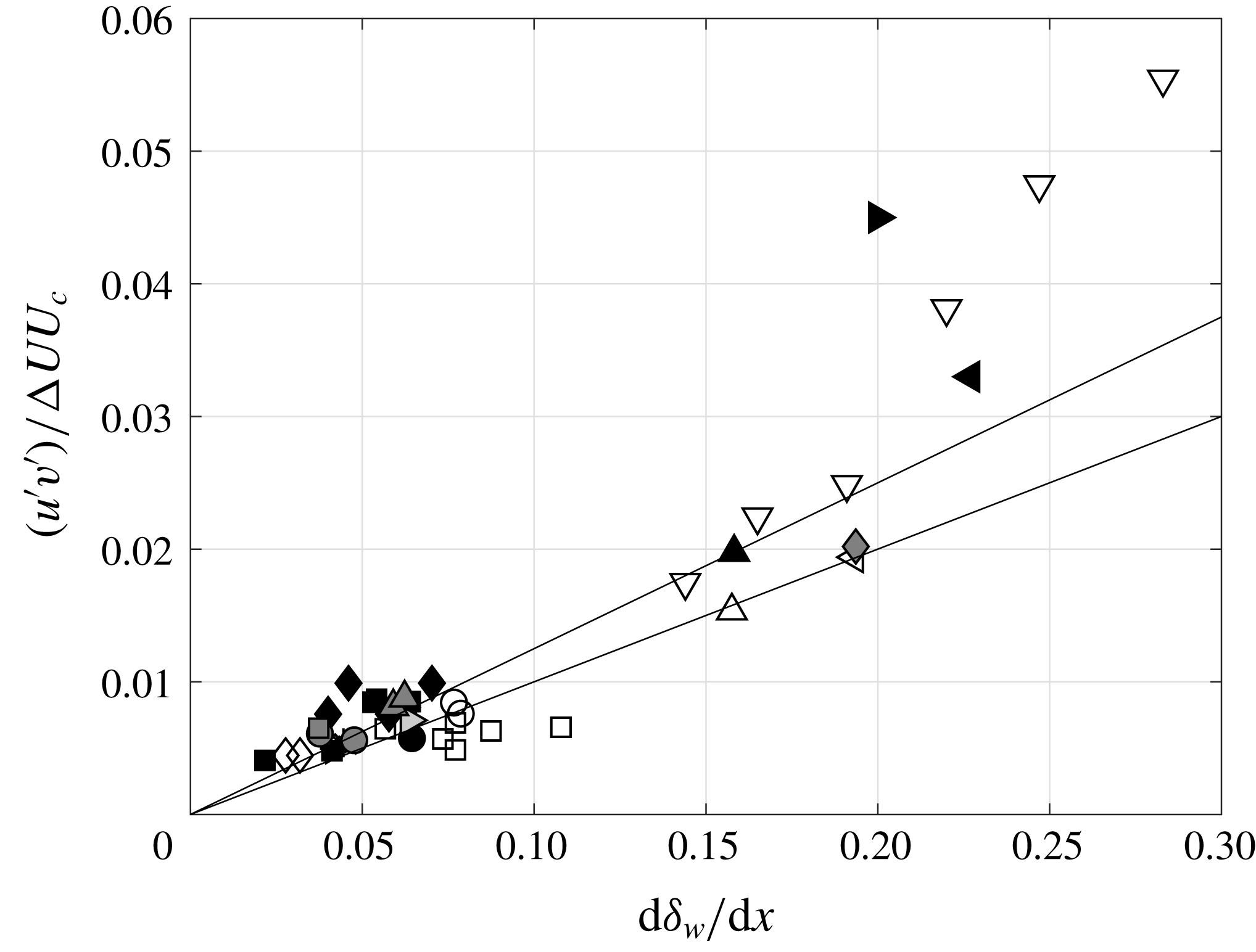
Now, we can check whether the spreading rate determination is in agreement with the measured value of turbulent shear stress. Barre, Quine & Dussauge (Reference Barre, Quine and Dussauge1994) proposed, on dimensional grounds, that it is possible to relate shear stress and spreading rates through the relation

(5.5) $$\begin{eqnarray}\frac{\text{d}\unicode[STIX]{x1D6FF}}{\text{d}x}=\frac{1}{K}\frac{\overline{-u^{\prime }v^{\prime }}_{max}}{\unicode[STIX]{x0394}UU_{c}}.\end{eqnarray}$$

Here $-\overline{u^{\prime }v^{\prime }}_{max}$ is the maximum shear stress in a section, $K$ is assumed to be a constant, $U_{c}$ is the convection velocity of the large-scale structures often determined from an isentropic assumption, and $\unicode[STIX]{x0394}U$ is the velocity difference through the layer. This relation is compared with experimental values in figure 11.

Figure 11.

Relation between spreading rate and turbulent shear stress. Symbols as in table 3.

Table 3.

List of symbols.

Figure 11 includes the measurements in subsonic and supersonic mixing layers. The abscissa represents the rate of spread based on vorticity thickness. Data are distributed over a large range of values, in particular for subsonic flows. The values reported by the authors have been reproduced without changes. A peculiar aspect is that the value of $\overline{-u^{\prime }v^{\prime }}$ is rather sensitive to the orientation of the frame of reference. This can be non-negligible for measurements by laser Doppler and PIV techniques, if the layer is not horizontal. However, this was accepted, but can contribute to increasing the scatter of data. Subsonic flows close to half-jet conditions ( $U_{2}\approx 0$ ) have a rate of growth close to $0.16$ . Subsonic layers with a rather large velocity ratio (typically $r=U_{2}/U_{1}\approx 0.6$ ) produce a smaller spreading rate. An interesting contribution is given by the layers with counterflow ( $U_{2}<0$ ) which have a large spreading rate ( ${>}0.16$ ), with a trend different from other (coflowing) data. Strykowski et al. (Reference Strykowski, Krothapalli and Jendoubi1996) and Forliti et al. (Reference Forliti, Tang and Strykowski2005) have shown that, in the counterflow regime, eddies have a different shape, probably resulting from a new instability and producing different entrainment rates. The supersonic data in canonical mixing layers have low spreading rates. Note that some experiments (Urban & Mungal Reference Urban and Mungal2001) did not indicate the spatial growth rate. In our case, the normalised spreading rate $\unicode[STIX]{x1D6F7}(M_{c})$ defined by the classical relationship

(5.6) $$\begin{eqnarray}\frac{\text{d}\unicode[STIX]{x1D6FF}_{\unicode[STIX]{x1D714}}}{\text{d}x}=\frac{1}{2}\left(\frac{\text{d}\unicode[STIX]{x1D6FF}_{\unicode[STIX]{x1D714}}}{\text{d}x}\right)_{ref}\frac{1-r(1+\sqrt{s})}{1+r\sqrt{s}}\,\unicode[STIX]{x1D6F7}(M_{c})\end{eqnarray}$$

has been used to determine $\text{d}\unicode[STIX]{x1D6FF}_{\unicode[STIX]{x1D714}}/\text{d}x$ . Two particular formulations for $\unicode[STIX]{x1D6F7}(M_{c})$ have been used: the Langley correlation (see Kline, Cantwell & Lilley Reference Kline, Cantwell and Lilley1980; Smits & Dussauge Reference Smits and Dussauge2006) and the proposal of Slessor, Zhuang & Dimotakis (Reference Slessor, Zhuang and Dimotakis2000). It was deemed that this should give a likely interval for $\text{d}\unicode[STIX]{x1D6FF}_{\unicode[STIX]{x1D714}}/\text{d}x$ .

Two lines of constant $K$ , $K=0.12\pm 0.02$ , have been drawn. It appears that, within experimental accuracy, the hypothesis of $K$ independent of the convective Mach number seems reasonable for coflowing mixing layers. From this viewpoint, the mechanisms of turbulent transport in such flows seem unaffected by the Mach number. For counterflows, the slope suggested by the subsonic data is much steeper; this is in agreement with the existence of a different flow regime, and a modification of entrainment, as claimed by Forliti et al. (Reference Forliti, Tang and Strykowski2005).

The results in the present shock–boundary layer interactions have been obtained by choosing $\unicode[STIX]{x0394}U$ as the velocity difference on both sides of the region where the large eddies are formed: $U_{2}$ is taken as the minimum value in the reverse flow, while $U_{1}$ is determined at the upper edge of this zone ( $y/\unicode[STIX]{x1D6FF}=0.5$ ) where $U_{1}/Ue\approx 0.6$ . They also refer to two assessments of the convection velocity $U_{c}$ , which has to be determined. A first assessment is given by the usual isentropic velocity:

(5.7) $$\begin{eqnarray}U_{c}=\frac{a_{1}U_{2}+a_{2}U_{1}}{a_{1}+a_{2}}=U_{1}\frac{\sqrt{s}+r}{1+\sqrt{s}}.\end{eqnarray}$$

In a first attempt, $U_{2}$ and $a_{2}$ are taken in the secondary flow, while $U_{1}$ and $a_{1}$ are the velocity and the sound speed in the external flow. The resulting values are denoted $U_{c,is1}$ in table 4. In a second determination, $U_{1}$ and $a_{1}$ are taken at the edge of the mixing layer where $y/\unicode[STIX]{x1D6FF}=0.5$ . The corresponding value is denoted $U_{c,is2}$ . These determinations have been compared to the velocity determined from wall pressure measurements in two points by Dupont et al. (Reference Dupont, Haddad and Debiève2006). A determination of the convection velocity has been made by Agostini et al. (Reference Agostini, Larchevêque, Dupont, Debiève and Dussauge2012) from the post-processing of the results of a large-eddy simulation (LES) of the interaction. The scope of this article was the determination of the sources of motion for the reflected shock wave. This led us to determine the convection velocity of the energetic eddies. Values ranging between 150 and $200~\text{m}~\text{s}^{-1}$ were found for the energetic eddies in the mixing layer. Table 4 shows that the experimental values, the numerical simulations and $U_{c,is2}$ are in reasonable agreement and that $U_{c,is1}$ is somewhat larger.

The three assessments of the convection velocity from the present definition of shear layer boundaries, wall pressure measurements and numerical simulations are consistent. This gives us some confidence in the definition of the edges of the mixing layer. However, the choice of $\unicode[STIX]{x0394}U$ and of $U_{c}$ has strong consequences on the normalisation of the shear stress: $\unicode[STIX]{x0394}U$ can be chosen at the edges of the shear layer; $U_{c,is2}$ seems a reasonable choice for the convection velocity, and this is retained. An assessment of the influence of the convection velocity can be made by choosing the maximum value found in the LES, i.e.  $200~\text{m}~\text{s}^{-1}$ . These result in a value 20 % lower for $9.5^{\circ }$ interaction, closer to the counterflow data; and a value 13 % lower for the $8^{\circ }$ interaction. The original use of this diagram was to check whether the dependence between spreading rate and shear stress was sensitive to compressibility. The conclusion, after considering coflow supersonic mixing layers, was that the compressibility effects were included entirely in the spreading rate itself, and not in the relation between the turbulent viscosity (or shear stress) and the rate of growth. This chart is therefore an indication of the relevance of the usual turbulent transport considerations for explaining growth of the shear layer. It can be seen that subsonic layers with counterflow have a particular behaviour, as explained by Forliti et al. (Reference Forliti, Tang and Strykowski2005) by a bifurcation in the solutions of the stability problem. The present results are scattered, probably because of the rather indirect determination of the spreading rate and also because of the difficulty in defining the edges of the shear layer and the convection velocity. However, the present results are also consistent with other data from subsonic and supersonic regime. It can be noted that, in the $8^{\circ }$ interaction, the velocity ratio is $r\approx -0.05$ , above the limit of bifurcation for subsonic flows, and is rather close to coflow results, while in the $9.5^{\circ }$ interaction, the velocity ratio is approximately $-0.1$ , i.e. beyond the threshold of bifurcation; the corresponding data point is closer to the counterflow experimental results. This suggests that, in the separation shear layer, as in canonical mixing layers, the effects of compressibility are included in the spreading rate itself and the turbulent fluxes follow the usual turbulent transport behaviour.

Table 4.

Convection velocity in the mixing layer $(\text{m}~\text{s}^{-1})$ .

Finally, a picture can be drawn from the results presented in this section: separation generates a mixing layer with a spreading rate typical of a counterflow shear layer. This spreading is consistent with the angle of deviation for the layer. Correspondingly, the resulting turbulent shear stress is in agreement with the trend imposed by the spreading rate. The relation between these two quantities seems to be the same at low speed and high speed. Compressibility effects are contained directly in these two quantities and not in the constant $K$ , which appears insensitive to Mach number, but sensitive to the nature of the flow (coflow versus counterflow) on the low-speed side. Some other aspects of compressibility are discussed in the next section.

Figure 12.

Ratio of normal stresses in subsosnic and supersonic mixing layers. Symbols as in table 3; – – –, $1/M_{c}^{2}$ ; ▸, present data; — $\bullet$ –, Langley consensus (Birch & Eggers Reference Birch and Eggers1973; Kline et al. Reference Kline, Cantwell and Lilley1980).

5.2 Anisotropy of the Reynolds stresses

Figure 12 presents the ratio of the maximum values of the variances $\overline{v^{\prime \,2}}/\overline{u^{\prime \,2}}$ versus convective Mach number. It can be seen in figure 7 that the vertical velocity fluctuations are rather small; the $\overline{v^{\prime \,2}}$ component is lower than the expected value.

Subsonic data in figure 12 have a value generally above $0.5$ , and some can even be close to $0.7$ . In fact, the dataset includes half-jets, coflowing and counterflowing shear layers, and mixing layers above separated zones, in particular backward-facing steps. These are the result of direct numerical simulations at lower Reynolds numbers (Pantano & Sarkar Reference Pantano and Sarkar2002; Helm, Martin & Dupont Reference Helm, Martin and Dupont2014) and LES at the nominal Reynolds number (Larchevêque et al. Reference Larchevêque, Dupont, De Martel, Garnier and Debiève2009). The diversity of conditions may explain the observed scatter: subsonic mixing layers above separated zones may have a modified anisotropy with larger $v^{\prime }$ ; note also that the counterflowing cases have a larger value for the ratio of the normal components. Moreover, as indicated in the previous section, the original data have been taken, without correction for the possible orientation of the frame of reference. This may explain some of the large values of the ratio $\overline{v^{\prime \,2}}/\overline{u^{\prime \,2}}$ . However, the evidence shows that the ratio is often larger than $0.5$ for subsonic flow conditions. For larger values of $M_{c}$ ( $M_{c}>0.3$ ), the data are all under this value. In particular, the present measurements, obtained at a convective Mach number close to 0.6, contribute significantly to this trend.

Brown & Roshko (Reference Brown and Roshko1974) proposed an interpretation using a dimensional analysis based on momentum and energy equations in which a balance between convective and pressure terms should be achieved. They used dimensional arguments in which $u^{\prime }\propto \unicode[STIX]{x0394}U$ and

(5.8) $$\begin{eqnarray}v^{\prime }\propto \unicode[STIX]{x1D6FF}^{\prime }U.\end{eqnarray}$$

This led to the prediction that the ratio of the normal stresses $\overline{v^{\prime \,2}}/\overline{u^{\prime \,2}}$ varies like $1/M^{2}$ . Their original paper, however, does not specify which characteristic Mach number should be used. A likely guess could be that the convective Mach number is the relevant parameter:

(5.9) $$\begin{eqnarray}\frac{\,\overline{v^{\prime \,2}}\,}{\,\overline{u^{\prime \,2}}\,}\propto \frac{1}{M_{c}^{2}}.\end{eqnarray}$$

In fact, it is possible to reformulate these considerations in a slightly different way. If the convection velocity of the large-scale eddies is the pertinent parameter, relation (5.8) can be formulated as follows:

(5.10) $$\begin{eqnarray}v^{\prime }\propto \unicode[STIX]{x1D6FF}^{\prime }U_{c}.\end{eqnarray}$$

Using the relation $\unicode[STIX]{x1D6FF}^{\prime }=\unicode[STIX]{x1D6FF}_{0}^{\prime }\unicode[STIX]{x1D6F7}(M_{c})(\unicode[STIX]{x0394}U/U_{c})$ (Papamoschou & Roshko Reference Papamoschou and Roshko1988), we obtain

(5.11) $$\begin{eqnarray}\frac{\,\overline{v^{\prime \,2}}\,}{\,\overline{u^{\prime \,2}}\,}\propto \unicode[STIX]{x1D6F7}^{2}(M_{c}),\end{eqnarray}$$

in which $\unicode[STIX]{x1D6F7}(M_{c})$ is the usual dimensionless spreading rate of the compressible mixing layer.

In figure 12, a line of slope $-2$ has been indicated, along with two representations of the spreading: the Langley curve (see e.g. Birch & Eggers Reference Birch and Eggers1973; Kline et al. Reference Kline, Cantwell and Lilley1980) and the proposal by Slessor et al. (Reference Slessor, Zhuang and Dimotakis2000). It appears that all these curves give a good reproduction of the overall trend and are in agreement with the Brown & Roshko (Reference Brown and Roshko1974) proposal. Obviously, the squared spreading rate follows an $M_{c}^{-2}$ law for $M_{c}\sim 0.8$ . It may be inferred that the observed decrease is a compressibility effect of the same sort as in canonical mixing layers. We also conclude that, even if the ratios $\overline{u^{\prime }v^{\prime }}/\overline{u^{\prime \,2}}$ or $\overline{u^{\prime }v^{\prime }}/k$ (where $k$ is the turbulent kinetic energy) are not very sensitive to compressibility (see e.g. Pantano & Sarkar Reference Pantano and Sarkar2002; Smits & Dussauge Reference Smits and Dussauge2006), the ratio of the normal Reynolds stresses can be affected at high speeds for convective Mach numbers close to 1. This consequence on the correlation coefficient between $u^{\prime }$ and $v^{\prime }$ is illustrated in figure 13 for the $9.5^{\circ }$ interaction. It shows that the absolute value of the correlation coefficient is somewhat larger than the results in subsonic layers. Again, as suggested by Brown & Roshko (Reference Brown and Roshko1974), this seems to be an effect of the pressure fluctuation terms in the energy equation.

Figure 13.

Correlation coefficient for velocity, expressed in the mixing layer coordinate system, $\unicode[STIX]{x1D703}=9.5^{\circ }$ .

6 Concluding remarks

The objective of this work was to reanalyse experiments in order to check that the free shear layer at the edge of a separated bubble in a shock–boundary layer interaction has properties in common with canonical mixing layers. The main problem was to extract this mixing layer from its turbulent environment. This was possible in the case of well-developed separation corresponding to shock–boundary layer interaction with a flow deviation of $9.5^{\circ }$ , and even in the case of smaller separation produced by an $8^{\circ }$ interaction. Once this new shear layer is correctly defined, the experimental results can be explained from the properties of canonical mixing layers. A first issue came from the unexpectedly large spreading rate, in spite of the stabilising effect of the Mach number. This has been explained by the presence of the counterflow in the separated zone. Mixing and spreading rate are enhanced by the counterflow, but compressibility moderates this effect. Moreover, the dependence between spreading rate and turbulent shear stress is essentially the same as in the canonical case, so that the development is related to turbulent transport. However, the experiment has produced evidence of compressibility effects. These had been hypothesised by Brown & Roshko (Reference Brown and Roshko1974) with possible consequences for the reduction of vertical velocity fluctuations; the present measurements are in agreement with a reformulation of the same idea, showing a variation in the anisotropy of the normal Reynolds stresses. Finally, all these elements show that, in many respects, the shear layer developed at the edge of a separated bubble in a separated shock reflection shares many features with the canonical ones, so that, finally, the approximations utilised by Piponniau et al. (Reference Piponniau, Dussauge, Debiève and Dupont2009) in the evaluation of the unsteadiness frequency remain safe for use.