2.1 Background

The second-order SFs of a velocity field are defined as follows (Monin & Yaglom Reference Monin and Yaglom1975; Pope Reference Pope2000):

(2.1) $$\begin{eqnarray}\displaystyle \unicode[STIX]{x1D60B}_{ij}(\boldsymbol{r},\boldsymbol{x},t)=\langle [u_{i}(\boldsymbol{x}+\boldsymbol{r},t)-u_{i}(\boldsymbol{x},t)][u_{j}(\boldsymbol{x}+\boldsymbol{r},t)-u_{j}(\boldsymbol{x},t)]\rangle , & & \displaystyle\end{eqnarray}$$

where $t$ is the time, $\boldsymbol{x}$ and $\boldsymbol{x}+\boldsymbol{r}$ are two spatial points, $r=|\boldsymbol{r}|$ is the distance between them, $u_{i}$ is the $i$ th component of the velocity vector $\boldsymbol{u}$ and $\langle q\rangle$ designates an ensemble-averaged value of an arbitrary scalar, vector or tensor quantity  $q$ . The tensor $\unicode[STIX]{x1D60B}_{ij}$ characterizes the second moments of the velocity difference across scales of size  $r$ . Accordingly, $\unicode[STIX]{x1D60B}_{ij}$ measures the energy of such and smaller eddies and, therefore, allows us to examine the energy distribution over the spatial scales directly in the physical space, contrary to energy spectra which deal with wavenumbers. Due to this feature, the second-order SFs are widely used both in theoretical and experimental studies of turbulent flows (Kolmogorov Reference Kolmogorov1941; Monin & Yaglom Reference Monin and Yaglom1975; Kuznetsov & Sabelnikov Reference Kuznetsov and Sabelnikov1990; Frisch Reference Frisch1995; Pope Reference Pope2000; Lesieur et al. Reference Lesieur, Métais and Comte2005; Davidson Reference Davidson2015).

In a homogeneous turbulent flow, the tensor $\unicode[STIX]{x1D60B}_{ij}$ does not depend on $\boldsymbol{x}$ and reduces to

(2.2) $$\begin{eqnarray}\displaystyle \unicode[STIX]{x1D60B}_{ij}(\boldsymbol{r},t)=2\langle u_{i}^{\prime }(\boldsymbol{x},t)u_{j}^{\prime }(\boldsymbol{x},t)\rangle -R_{ij}(\boldsymbol{r},t)-R_{ji}(\boldsymbol{r},t), & & \displaystyle\end{eqnarray}$$

where $q^{\prime }(\boldsymbol{x},t)\equiv q(\boldsymbol{x},t)-\langle q\rangle (t)$ for any scalar, vector or tensor quantity $q$ and

(2.3) $$\begin{eqnarray}\displaystyle R_{ij}(\boldsymbol{r},t)=R_{ji}(-\boldsymbol{r},t)=\langle u_{i}^{\prime }(\boldsymbol{x}+\boldsymbol{r},t)u_{j}^{\prime }(\boldsymbol{x},t)\rangle & & \displaystyle\end{eqnarray}$$

are correlation functions (Monin & Yaglom Reference Monin and Yaglom1975; Pope Reference Pope2000). Consequently, in a homogeneous turbulent flow, the SFs are directly linked with the correlation functions $R_{ij}(\boldsymbol{r},t)$ , which are used to obtain energy spectra. If the distance $r$ is large when compared to an integral length scale $L$ of the turbulence, then, the correlation functions vanish and $\unicode[STIX]{x1D60B}_{ij}\rightarrow 2\langle u_{i}^{\prime }(\boldsymbol{x},t)u_{j}^{\prime }(\boldsymbol{x},t)\rangle$ or $\unicode[STIX]{x1D60B}_{ij}\rightarrow 2u^{\prime 2}\unicode[STIX]{x1D6FF}_{ij}$ if the turbulence is not only homogeneous, but also isotropic. Here, $\unicode[STIX]{x1D6FF}_{ij}$ is the Kronecker delta, $u^{\prime }(t)=\sqrt{u_{k}^{\prime }(\boldsymbol{x},t)u_{k}^{\prime }(\boldsymbol{x},t)/3}$ is the r.m.s. turbulent velocity and the summation convention applies for repeated indexes. In an inhomogeneous turbulent flow, which is more relevant to combustion, the relationship between the structure and correlation functions is not straightforward. Accordingly, the SFs and energy spectra may convey different (complementary) information in such a case.

In incompressible homogeneous isotropic turbulence (Monin & Yaglom Reference Monin and Yaglom1975; Pope Reference Pope2000), the tensor $\unicode[STIX]{x1D60B}_{ij}(\boldsymbol{r},t)$ is fully determined by a single scalar longitudinal SF

(2.4) $$\begin{eqnarray}\displaystyle D_{LL}(r,t)\equiv \langle [\boldsymbol{u}_{L}(\boldsymbol{x}+\boldsymbol{r},t)-\boldsymbol{u}_{L}(\boldsymbol{x},t)]^{2}\rangle , & & \displaystyle\end{eqnarray}$$

i.e.

(2.5) $$\begin{eqnarray}\displaystyle \unicode[STIX]{x1D60B}_{ij}(\boldsymbol{r},t)=D_{NN}(r,t)\unicode[STIX]{x1D6FF}_{ij}+[D_{L}(r,t)-D_{NN}(r,t)]\frac{r_{i}r_{j}}{r^{2}}, & & \displaystyle\end{eqnarray}$$

with the transverse SF

(2.6) $$\begin{eqnarray}\displaystyle D_{NN}(r,t)\equiv \langle [\boldsymbol{u}_{N}(\boldsymbol{x}+\boldsymbol{r},t)-\boldsymbol{u}_{N}(\boldsymbol{x},t)]^{2}\rangle & & \displaystyle\end{eqnarray}$$

being equal to

(2.7) $$\begin{eqnarray}\displaystyle D_{NN}(r,t)=D_{LL}(r,t)+\frac{r}{2}\frac{\unicode[STIX]{x2202}D_{LL}}{\unicode[STIX]{x2202}r}. & & \displaystyle\end{eqnarray}$$

Here, $\boldsymbol{u}_{L}=\boldsymbol{r}(\boldsymbol{u}\boldsymbol{\cdot }\boldsymbol{r})/r^{2}$ is the component of the velocity vector $\boldsymbol{u}$ in the direction of vector  $\boldsymbol{r}$ , and $\boldsymbol{u}_{N}$ is the component of the velocity vector normal to  $\boldsymbol{r}$ .

Within the framework of the Kolmogorov theory of the inertial range (Kolmogorov Reference Kolmogorov1941), $D_{LL}(r)=C_{2}(\langle \unicode[STIX]{x1D700}\rangle r)^{2/3}$ and $D_{NN}(r)=4D_{LL}(r)/3$ , with $C_{2}$ being a universal constant. Here, $\unicode[STIX]{x1D700}=2\unicode[STIX]{x1D708}\unicode[STIX]{x1D61A}_{ij}\unicode[STIX]{x1D61A}_{ij}$ is the viscous dissipation rate, $\unicode[STIX]{x1D708}$ is the kinematic viscosity of the fluid and $\unicode[STIX]{x1D61A}_{ij}=0.5(\unicode[STIX]{x2202}u_{i}/\unicode[STIX]{x2202}x_{j}+\unicode[STIX]{x2202}u_{j}/\unicode[STIX]{x2202}x_{i})$ is the rate-of-strain tensor. Therefore, consistency of DNS conditions with the Kolmogorov theory of turbulence can be checked not only by comparing the energy spectrum with the $5/3$ law (Obukhov Reference Obukhov1941), as commonly done in combustion DNS, but also by examining (i) in which range of scales $l$ (if any) a ratio of $D_{LL}(r)/(\langle \unicode[STIX]{x1D700}\rangle r)^{2/3}$ or $D_{NN}(r)/(\langle \unicode[STIX]{x1D700}\rangle r)^{2/3}$ is independent of  $r$ , (ii) whether or not this range of scales is consistent with $\unicode[STIX]{x1D702}\ll l\ll L$ and (iii) whether or not the computed constant ratio is consistent with the known value of $C_{2}$ (or $4C_{2}/3$ , respectively). Here, $\unicode[STIX]{x1D702}=(\unicode[STIX]{x1D708}^{3}/\langle \unicode[STIX]{x1D700}\rangle )^{1/4}$ is the Kolmogorov length scale.

If $r$ is sufficiently small, e.g. $r\ll \unicode[STIX]{x1D702}$ , the two-point velocity difference may be evaluated using Taylor expansion, i.e. $\unicode[STIX]{x1D60B}_{ij}\propto \langle (\unicode[STIX]{x2202}u_{i}^{\prime }/\unicode[STIX]{x2202}x_{k})(\unicode[STIX]{x2202}u_{j}^{\prime }/\unicode[STIX]{x2202}x_{l})\rangle r_{k}r_{l}$ in a general case or $D_{LL}\rightarrow (\langle \unicode[STIX]{x1D700}\rangle /15\unicode[STIX]{x1D708})r^{2}$ in locally homogeneous isotropic turbulence (Kolmogorov Reference Kolmogorov1941).

2.2 Conditioned structure functions

Within a premixed turbulent flame brush, local velocity is increased due to a decrease in the local density  $\unicode[STIX]{x1D70C}$ , caused by combustion-induced thermal expansion. Often, such density changes are localized to thin zones and the local velocity normal to the zone jumps at the burned side of the zone when compared to the unburned side, with such effects being most pronounced in the flamelet regime of premixed turbulent combustion (Bray Reference Bray1995; Lipatnikov & Chomiak Reference Lipatnikov and Chomiak2010; Sabelnikov & Lipatnikov Reference Sabelnikov and Lipatnikov2017). Because such a velocity jump is hardly associated with turbulence described by the Kolmogorov theory, the use of mean (ensemble-averaged) quantities for characterizing turbulence in premixed flames appears to be a flawed approach (Lipatnikov Reference Lipatnikov2009; Lipatnikov & Chomiak Reference Lipatnikov and Chomiak2010; Sabelnikov & Lipatnikov Reference Sabelnikov and Lipatnikov2017), at least in the flamelet combustion regime. To resolve the problem, flow characteristics conditioned to an unburned (or burned) mixture are often considered instead of mean flow characteristics, as reviewed elsewhere (Lipatnikov & Chomiak Reference Lipatnikov and Chomiak2010). However, as far as energy spectra obtained from spatial correlations computed in DNS are concerned (Kolla et al. Reference Kolla, Hawkes, Kerstein, Swaminathan and Chen2014; Lipatnikov et al. Reference Lipatnikov, Chomiak, Sabelnikov, Nishiki and Hasegawa2015b ; Towery et al. Reference Towery, Poludnenko, Urzay, O’Brien, Ihme and Hamlington2016; O’Brien et al. Reference O’Brien, Towery, Hamlington, Ihme, Poludnenko and Urzay2017), the present authors are aware on a single study of the conditioned spectra (Lipatnikov et al. Reference Lipatnikov, Chomiak, Sabelnikov, Nishiki and Hasegawa2015b ), with that study being restricted to the leading edges of mean flame brushes. The SFs offer an opportunity to feel the gap and to gain insight into the conditioned two-point statistics of the turbulent velocity field.

For this purpose, we will follow an approach developed earlier to study intermittency in non-reacting turbulent flows (Kuznetsov & Sabelnikov Reference Kuznetsov and Sabelnikov1990). Because the aforementioned velocity jump is associated with some kind of intermittency, i.e. unburned–burned intermittency, extension of the approach to premixed flames is straightforward (Sabelnikov et al. Reference Sabelnikov, Lipatnikov, Nishiki and Hasegawa2019).

Let us (i) characterize the state of a reacting mixture with a single combustion progress variable $c(\boldsymbol{x},t)$ (Bray Reference Bray1995), which monotonically increases from zero in fresh reactants to unity in equilibrium combustion products, and (ii) introduce $K$ indicator functions $I_{k}(\boldsymbol{x},t)$ , $k=1,\ldots ,K$ , such that $I_{k}(\boldsymbol{x},t)=1$ if $c_{k-1}<c(\boldsymbol{x},t)\leqslant c_{k}$ and vanishes otherwise. Here, $c_{0}=0$ (fresh) reactants and $c_{K}=1$ (equilibrium products). Obviously, the following identity

(2.8) $$\begin{eqnarray}\displaystyle \mathop{\sum }_{k=1}^{K}I_{k}(\boldsymbol{x},t)=1 & & \displaystyle\end{eqnarray}$$

holds at any point at any instant. Then, for any bounded, single-point, scalar, vector or tensor quantity $q(\boldsymbol{x},t)$ ,

(2.9) $$\begin{eqnarray}\displaystyle \langle q\rangle (\boldsymbol{x},t) & = & \displaystyle \left\langle q(\boldsymbol{x},t)\mathop{\sum }_{k=1}^{K}I_{k}(\boldsymbol{x},t)\right\rangle =\left\langle \mathop{\sum }_{k=1}^{K}q(\boldsymbol{x},t)I_{k}(\boldsymbol{x},t)\right\rangle \nonumber\\ \displaystyle & = & \displaystyle \mathop{\sum }_{k=1}^{K}\langle q(\boldsymbol{x},t)I_{k}(\boldsymbol{x},t)\rangle =\mathop{\sum }_{k=1}^{K}\mathit{P}_{k}(\boldsymbol{x},t)\langle q\rangle _{k}(\boldsymbol{x},t),\end{eqnarray}$$

and, for any two-point scalar, vector or tensor quantity $Q_{AB}=Q(\boldsymbol{x}_{A},\boldsymbol{x}_{B},t)$ ,

(2.10) $$\begin{eqnarray}\displaystyle \langle Q_{AB}\rangle =\left\langle Q_{AB}\left(\mathop{\sum }_{k=1}^{K}I_{A,k}\right)\left(\mathop{\sum }_{l=1}^{K}I_{B,l}\right)\right\rangle =\mathop{\sum }_{k=1}^{K}\mathop{\sum }_{l=1}^{K}\langle Q_{AB}\rangle _{kl}\mathit{P}_{kl}. & & \displaystyle\end{eqnarray}$$

Henceforth, dependencies of various quantities on time $t$ and spatial coordinates $\boldsymbol{x}$ are not specified unless the opposite is required, $q_{A}$ and $q_{B}$ designate values of  $q$ , measured at points $\boldsymbol{x}_{A}$ and $\boldsymbol{x}_{B}=\boldsymbol{x}_{A}+\boldsymbol{r}$ , respectively, at the same instant $t$ , $\langle q\rangle$ is the mean value of $q$ , $\langle q\rangle _{k}=\langle qI_{k}\rangle /\mathit{P}_{k}$ is the value of $q$ conditioned to the $k$ th state of the mixture, i.e. $c_{k-1}<c(\boldsymbol{x},t)\leqslant c_{k}$ , $\mathit{P}_{k}(\boldsymbol{x},t)=\langle I_{k}\rangle$ is the probability of finding this state at point $\boldsymbol{x}$ at instant  $t$ , $\langle Q_{AB}\rangle _{kl}=\langle Q_{AB}I_{A,k}I_{B,l}\rangle /\mathit{P}_{kl}$ is conditioned to the $k$ th state of the mixture at point A and the $l$ th sate of the mixture at point B and $\mathit{P}_{kl}\equiv \langle I_{A,k}I_{B,l}\rangle$ is the probability that the mixture states $k$ and $l$ are recorded at points $\boldsymbol{x}_{A}$ and $\boldsymbol{x}_{B}$ , respectively, at the same instant.

If $Q_{AB}$ designates tensor $(u_{B,i}-u_{A,i})(u_{B,j}-u_{A,j})$ , then, (2.10) reads

(2.11) $$\begin{eqnarray}\displaystyle \unicode[STIX]{x1D60B}_{ij}=\mathop{\sum }_{k=1}^{K}\mathop{\sum }_{l=1}^{K}\unicode[STIX]{x1D60B}_{ij,kl}\mathit{P}_{kl}, & & \displaystyle\end{eqnarray}$$

where subscripts $i$ and $j$ refer to spatial coordinates, subscripts $k$ and $l$ refer to the state of the mixture and

(2.12) $$\begin{eqnarray}\displaystyle \unicode[STIX]{x1D60B}_{ij,kl}\equiv \langle (u_{B,i}-u_{A,i})(u_{B,j}-u_{A,j})I_{B,l}I_{A,k}\rangle /\mathit{P}_{kl} & & \displaystyle\end{eqnarray}$$

are conditioned SFs.

If $K=3$ , $c_{1}=\unicode[STIX]{x1D716}\ll 1$ and $c_{2}=1-\unicode[STIX]{x1D716}$ , then, there are six different conditioned structure function tensors and six different probabilities:

1. (i) $\unicode[STIX]{x1D60B}_{ij,11}$ or $\unicode[STIX]{x1D60B}_{ij,uu}$ and $\mathit{P}_{11}$ or $\mathit{P}_{uu}$ (fresh reactants at both points);

2. (ii) $\unicode[STIX]{x1D60B}_{ij,22}$ or $\unicode[STIX]{x1D60B}_{ij,ff}$ and $\mathit{P}_{22}$ or $\mathit{P}_{ff}$ (intermediate states of the mixture at both points);

3. (iii) $\unicode[STIX]{x1D60B}_{ij,33}$ or $\unicode[STIX]{x1D60B}_{ij,bb}$ and $\mathit{P}_{33}$ or $\mathit{P}_{bb}$ (equilibrium products at both points);

4. (iv) $\unicode[STIX]{x1D60B}_{ij,12}$ or $\unicode[STIX]{x1D60B}_{ij,uf}$ and $\mathit{P}_{12}$ or $\mathit{P}_{uf}$ (the reactants at one point, but an intermediate state at another point);

5. (v) $\unicode[STIX]{x1D60B}_{ij,13}$ or $\unicode[STIX]{x1D60B}_{ij,ub}$ and $\mathit{P}_{13}$ or $\mathit{P}_{ub}$ (the reactants at one point, but the products at another point);

6. (vi) $\unicode[STIX]{x1D60B}_{ij,23}$ or $\unicode[STIX]{x1D60B}_{ij,fb}$ and $\mathit{P}_{23}$ or $\mathit{P}_{fb}$ (an intermediate state at one point, but the products at another point).

Here, standard subscripts $u$ and $b$ designate unburned (fresh) reactants, i.e. $k=1$ and $0\leqslant c(\boldsymbol{x},t)\leqslant \unicode[STIX]{x1D716}$ , and burned (equilibrium) products, i.e. $k=3$ and $1-\unicode[STIX]{x1D716}<c(\boldsymbol{x},t)\leqslant 1$ , whereas intermediate states of the mixture, i.e. $k=2$ and $\unicode[STIX]{x1D716}<c(\boldsymbol{x},t)\leqslant 1-\unicode[STIX]{x1D716}$ , are designated with subscript $f$ associated with flames or flamelets.

Exact transport equations for $\unicode[STIX]{x1D60B}_{ij,kl}$ can be derived using the continuity and Navier–Stokes equations in a general unsteady, inhomogeneous and anisotropic case, as shown in appendix A for $\unicode[STIX]{x1D60B}_{ij,11}$ . Since the obtained equation is cumbersome and involves a number of unclosed terms, analysis of it (or transport equations for other conditioned SFs $\unicode[STIX]{x1D60B}_{ij,kl}$ ) appears to be warranted provided that the capabilities of the newly introduced conditioned SF approach to advance the understanding of turbulent reacting flows is demonstrated. Accordingly, the rest of the paper aims at showing that even simple and direct application of the proposed approach to analysing DNS data can substantially advance our understanding of flame–turbulence interaction. Analysis of the derived transport equation is a subject for future study.

The largest part of the following analysis will be restricted to the aforementioned six conditioned SFs and three states of the mixture. Nevertheless, one more SF tensor $\unicode[STIX]{x1D60B}_{ij,ww}(\boldsymbol{x},\boldsymbol{r})$ and one more probability $\mathit{P}_{ww}(\boldsymbol{x},\boldsymbol{r})$ , both conditioned to the heat-release zone (HRZ), i.e. to $c_{w,1}<c(\boldsymbol{x},t)\leqslant c_{w,2}$ , will also be addressed in the following. Here, the boundaries of the zone are associated with a threshold value of the rate $W(c)$ of product creation, e.g. $W(c_{w,1})=W(c_{w,2})=0.5\max \{W(c)\}$ , and subscript $w$ indicates a significant reaction rate. Investigation of this SF can shed a new light on the following fundamental issue. Two-dimensional (2-D) DNS study (Poinsot, Veynante & Candel Reference Poinsot, Veynante and Candel1991) of the interaction of a laminar premixed flame with a vortex pair and experimental investigations (Roberts et al. Reference Roberts, Driscoll, Drake and Goss1993) of the interaction of a laminar premixed flame with a laminar toroidal vortex have shown that isolated small-scale laminar vortices are inefficient in perturbing the flame HRZ. As reviewed elsewhere (Renard et al. Reference Renard, Thévenin, Rolon and Candel2000; Kadowaki & Hasegawa Reference Kadowaki and Hasegawa2005), this finding was confirmed in subsequent simulations and measurements of laminar flame–vortex interaction. Accordingly, the smallest-scale turbulent eddies are often hypothesized to be inefficient in stretching HRZs in premixed flames, in particular, because such eddies rapidly disappear due to dilatation and an increase in viscosity within the flame preheat zone. Recent 2-D experimental data by Wabel, Skiba & Driscoll (Reference Wabel, Skiba and Driscoll2018) indicate two trends, i.e. (i) an integral turbulence length scale is increased across flame preheat zones, whereas (ii) the turbulence level does not decrease therein, which (trends) appear to indirectly support the hypothesis (Poinsot et al. Reference Poinsot, Veynante and Candel1991; Roberts et al. Reference Roberts, Driscoll, Drake and Goss1993; Renard et al. Reference Renard, Thévenin, Rolon and Candel2000; Driscoll Reference Driscoll2008) on the disappearance of the smallest-scale turbulent eddies within flame preheat zones. The aforementioned conditioned SF $\unicode[STIX]{x1D60B}_{ij,ww}(\boldsymbol{x},\boldsymbol{r})$ appears to be perfectly suited to directly exploring the hypothesis.

4.1 Typical structure functions

Typical mean (dots) and conditioned (lines) SFs are shown in figures 1–3. These data were computed in the middle of the flame brushes, i.e. at distance $x^{\ast }$ characterized by the minimal difference $|\langle c\rangle (x)-0.5|$ , in order for the probabilities $\mathit{P}_{kl}(\langle c\rangle ,r)$ to be significant, see figure 4, thus, allowing us to obtain solid statistics. The SFs are normalized using the square $|\unicode[STIX]{x0394}u|_{L}^{2}$ of the normal velocity jump $|\unicode[STIX]{x0394}u|_{L}=(\unicode[STIX]{x1D70E}-1)S_{L}$ across the laminar flame ( $|\unicode[STIX]{x0394}u|_{L}^{2}=15.35$ and $0.39~\text{m}^{2}~\text{s}^{-2}$ in cases H and L, respectively). The distance $r$ is normalized using the distance $\unicode[STIX]{x1D6FF}_{\unicode[STIX]{x1D716}}$ between iso-surfaces $c=\unicode[STIX]{x1D716}$ and $c=1-\unicode[STIX]{x1D716}$ in the unperturbed laminar flame ( $\unicode[STIX]{x1D6FF}_{\unicode[STIX]{x1D716}}=0.28$ and 0.22 mm in cases H and L, respectively). This distance is used instead of $\unicode[STIX]{x1D6FF}_{L}$ , because reactant–product SFs should vanish if $r<\unicode[STIX]{x1D6FF}_{\unicode[STIX]{x1D716}}$ provided that the flamelets retain the local structure of the unperturbed laminar flame. The laminar flame scales are chosen, because a substantial part of subsequent discussion, e.g. see § 4.2, will address the behaviour of reactant–product SFs at distances close to  $\unicode[STIX]{x1D6FF}_{\unicode[STIX]{x1D716}}$ .

To illustrate the capabilities of the SF approach, let us note certain trends indicated in figures 1–3.

Figure 1.

Normalized conditioned (lines) and mean (dots) longitudinal SFs $D_{yz,L}[\langle c\rangle (x^{\ast }),r/\unicode[STIX]{x1D6FF}_{\unicode[STIX]{x1D716}}]/|\unicode[STIX]{x0394}u|_{L}^{2}$ for the transverse velocity, obtained in the middle of flame brush in case (a) H or (b) L.

Figure 2.

Normalized conditioned (lines) and mean (dots) transverse SFs $D_{xx,T}[\langle c\rangle (x^{\ast }),r/\unicode[STIX]{x1D6FF}_{\unicode[STIX]{x1D716}}]/|\unicode[STIX]{x0394}u|_{L}^{2}$ for the axial velocity, obtained in the middle of flame brush in case (a) H or (b) L.

Figure 3.

Normalized conditioned (lines) and mean (dots) transverse SFs $D_{yz,T}[\langle c\rangle (x^{\ast }),r/\unicode[STIX]{x1D6FF}_{\unicode[STIX]{x1D716}}]/|\unicode[STIX]{x0394}u|_{L}^{2}$ for the transverse velocity, obtained in the middle of flame brush in case (a) H or (b) L.

Figure 4.

Probabilities $\mathit{P}_{kl}[\langle c\rangle (x^{\ast }),r/\unicode[STIX]{x1D6FF}_{\unicode[STIX]{x1D716}}]$ obtained in the middle of flame brush in case (a) H or (b) L.

First, the mean SFs differ substantially from the conditioned SFs, thus, showing that the velocity jumps associated with the unburned–burned intermittency strongly change the two-point statistics of the velocity field within a premixed turbulent flame brush. Therefore, the results plotted in figures 1–3 call for investigation of the conditioned fields in order to properly characterize the aforementioned two-point statistics.

Second, the magnitudes of almost all SFs are significantly increased by the density ratio  $\unicode[STIX]{x1D70E}$ , cf. results obtained in cases H and L. (The higher magnitude of reactant–reactant (i.e.  $uu$ ) SFs computed in case H is associated with a shorter time during which the turbulence decays upstream of the mean flame brush, as discussed in detail elsewhere (Lipatnikov et al. Reference Lipatnikov, Chomiak, Sabelnikov, Nishiki and Hasegawa2018a ). This time is shorter in case H when compared to case L, because the turbulent flame speed $S_{t}$ and the mean inlet velocity are higher in the former case, whereas distances from the inlet to the flame leading edges are approximately equal in the two cases.) This trend is expected because variations in the density increase the variability of the velocity field and, consequently, the velocity differences between two points. The discussed difference between cases H and L is much more pronounced if different mixture states are observed at the two points, i.e. if the difference in $\unicode[STIX]{x1D70C}_{A}$ and $\unicode[STIX]{x1D70C}_{B}$ is large, cf. curves  $ub$ , $uf$ or  $fb$ in cases H and L.

Third, in case H, the reactant–reactant SFs, see curves $uu$ plotted by the dashed lines in figures 1(a) and 2(a), have the lowest magnitudes among all conditioned SFs, because the reactants are least subjected to thermal-expansion effects.

Fourth, curves $ub$ plotted by the solid lines in figure 2 show that the transverse reactant–product SF $D_{xx,T,ub}$ for the axial velocity has the largest magnitude among all SFs plotted in figures 1–3, with the effect being much more pronounced in case H. These trends are associated with strong (weak) axial acceleration of low-density products (high-density reactants) by the combustion-induced mean axial pressure gradient $\langle \unicode[STIX]{x1D735}_{x}p\rangle$ , which is significantly stronger in case H. In particular, an increase in the reactant–product SF $D_{xx,T,ub}$ with distance $r$ may be attributed to a mechanism highlighted by Scurlock & Grover (Reference Scurlock and Grover1953) and by Libby & Bray (Reference Libby and Bray1981). For instance, if the reactant coordinate $\boldsymbol{x}_{A}$ is kept constant, but the distance $r$ is increased, the axial distance between low-density products at point B and the flamelet surface is likely to be increased. Therefore, the products have strongly been accelerated by $\unicode[STIX]{x1D70C}^{-1}\langle \unicode[STIX]{x1D735}_{x}p\rangle$ during a longer time required to reach a more distant point B. Consequently, their axial velocity is higher at that point.

Fifth, a decrease in the longitudinal reactant–product SF $D_{yz,L,ub}$ with  $r$ , see curves $ub$ plotted by the solid lines in figure 1, may be attributed to the same mechanism bearing in mind that the studied flames generate a mean axial pressure gradient $\langle \unicode[STIX]{x1D735}_{x}p\rangle$ , but do not induce a mean transverse pressure gradient. Accordingly, when the products are accelerated by $\langle \unicode[STIX]{x1D735}_{x}p\rangle$ in the axial direction, the magnitude of their transverse velocity decreases due to mass conservation, because the product density is constant.

Sixth, as discussed in detail elsewhere (Lipatnikov et al. Reference Lipatnikov, Nishiki and Hasegawa2015c ), the local flamelet structure is weakly perturbed (when compared to the laminar flame) under conditions of the present DNS at $\langle c\rangle (x^{\ast })\approx 0.5$ . Therefore, reactants and products cannot simultaneously be observed at two points separated by a distance $r$ that is substantially less than $\unicode[STIX]{x1D6FF}_{\unicode[STIX]{x1D716}}$ . Accordingly, the probability $\mathit{P}_{ub}$ vanishes if $r/\unicode[STIX]{x1D6FF}_{\unicode[STIX]{x1D716}}<1$ , see curves $ub$ plotted by the solid lines in figure 4. Nevertheless, at $r/\unicode[STIX]{x1D6FF}_{\unicode[STIX]{x1D716}}\approx 1$ , the probability is small, but finite, and there is a jump of the longitudinal reactant–product SF $D_{yz,L,ub}$ , see curves $ub$ plotted by the solid lines in figure 1. This jump is attributed to local flow acceleration across flamelets in the directions that are locally normal to the flamelets. The location of the jump at $r/\unicode[STIX]{x1D6FF}_{\unicode[STIX]{x1D716}}\approx 1$ indicates the appearance of flamelets that are locally normal to the $y$ or $z$ coordinate axis. Indeed, if a flamelet is significantly inclined to both transverse axes, the distance between the reactant and product edges of the flamelet, counted in the $y$ or $z$ direction, is larger than the distance $\unicode[STIX]{x1D6FF}_{\unicode[STIX]{x1D716}}$ counted between the two edges in the locally normal direction.

Seventh, a significant increase in the longitudinal product–product SF $D_{yz,L,bb}$ with $r$ observed in case H, see curve $bb$ plotted by the dotted-dashed line in figure 1(a), might result from the opposite directions of the transverse velocities $v$ (or $w$ ) induced due to thermal expansion at opposite sides of a layer that is filled by the reactants and is almost parallel to the $x$ -axis. Such finger-like structures were observed by analysing the present DNS data (Lipatnikov et al. Reference Lipatnikov, Chomiak, Sabelnikov, Nishiki and Hasegawa2015a , Reference Lipatnikov, Chomiak, Sabelnikov, Nishiki and Hasegawa2018a ). In case L, an increase in the longitudinal product–product SF $D_{yz,L,bb}$ with $r$ is also observed, but the magnitude of the effect is much lower due to significantly weaker flow acceleration within flamelets.

Eighth, the transverse flamelet–product $D_{xx,T,fb}$ and reactant–flamelet $D_{xx,T,uf}$ SFs behave similarly to the reactant–product SF $D_{xx,T,ub}$ , cf. curves  $fb$ , $uf$ and  $ub$ , respectively, in figure 2, but have smaller magnitudes, because the density difference is largest for the reactant–product pairs of points.

Ninth, differences between SFs conditioned to various events are smallest in the case of SF $D_{yz,T}$ , because $\langle \unicode[STIX]{x1D735}_{y}p\rangle =\langle \unicode[STIX]{x1D735}_{z}p\rangle =0$ and flamelets normal to the $y$ (or  $z$ ) component of the local velocity field do not induce a pressure gradient in the transverse $z$ (or  $y$ , respectively) direction. Accordingly, the influence of combustion on the SFs is least pronounced for the transverse SF $D_{yz,T}$ for the tangential velocities $v$ and $w$ in the selected coordinate framework.

Thus, the considered examples show that (i) the conditioned SFs convey a large amount of information on the influence of combustion-induced thermal expansion on velocity fields in premixed turbulent flames and (ii) this influence is significantly reduced when the density ratio is decreased. Although the trends discussed above might be claimed to be expected, the use of the SFs offers an opportunity to reveal an apparently surprising effect examined in the next subsection.

4.2 Local shear layers

Figures 1–3 show that the reactant–product SFs vanish at $r/\unicode[STIX]{x1D6FF}_{\unicode[STIX]{x1D716}}<1$ , but have finite or even peak values close to $r/\unicode[STIX]{x1D6FF}_{\unicode[STIX]{x1D716}}=1$ . Thus, if $r>\unicode[STIX]{x1D6FF}_{\unicode[STIX]{x1D716}}$ , then, independently of a transverse direction ( $y$ or  $z$ ), there are pairs of points $(\boldsymbol{x}_{A},\boldsymbol{x}_{B})$ such that (i) both points lie on a line parallel to a transverse coordinate axis, (ii) distance $r$ between the two points is close to $\unicode[STIX]{x1D6FF}_{\unicode[STIX]{x1D716}}$ and (iii)  $c(\boldsymbol{x}_{A},t)<0.05$ and $c(\boldsymbol{x}_{B},t)>0.95$ or vice versa. However, the probability of such events is low if $r$ is close to $\unicode[STIX]{x1D6FF}_{\unicode[STIX]{x1D716}}$ , see solid line in figure 4. As already argued in the previous subsection, such events are associated with flamelets that are locally normal to a transverse coordinate axis $y$ or  $z$ .

Moreover, at the lowest $r\approx \unicode[STIX]{x1D6FF}_{\unicode[STIX]{x1D716}}$ associated with a finite probability $\mathit{P}_{ub}>0$ , the normalized reactant–product SF $D_{yz,T,ub}/|\unicode[STIX]{x0394}u|_{L}^{2}$ has a very small magnitude of approximately 0.05 at $\langle c\rangle =0.5$ in case H. If flamelets that control the SF at $r\approx \unicode[STIX]{x1D6FF}_{\unicode[STIX]{x1D716}}$ were inclined to both transverse axes $y$ and  $z$ , then, contributions from $D_{yy,T,ub}$ , i.e. difference in $v$ in the $z$ -direction, and from $D_{zz,T,ub}$ , i.e. difference in $w$ in the $y$ -direction, would yield a significantly larger $D_{yz,T,ub}/|\unicode[STIX]{x0394}u|_{L}^{2}$ due to jumps of the locally normal components of $v$ and $w$ across the flamelets. Consequently, the computed small magnitude of $D_{yz,T,ub}/|\unicode[STIX]{x0394}u|_{L}^{2}$ at $r\approx \unicode[STIX]{x1D6FF}_{\unicode[STIX]{x1D716}}$ also indicates that flamelets associated with the lowest distance $r_{y}$ or $r_{z}$ between the reactants and products are almost normal to the $y$ or $z$ -axis, respectively.

Nevertheless, the peak value of $D_{yz,L,ub}[\langle c\rangle (x^{\ast }),r/\unicode[STIX]{x1D6FF}_{\unicode[STIX]{x1D716}}]$ , obtained at $r\approx \unicode[STIX]{x1D6FF}_{\unicode[STIX]{x1D716}}$ , see curve $ub$ in figure 1(a), and, therefore, controlled by such ‘locally normal’ (to the $y$ or $z$ -axis) flamelets, is substantially less than $|\unicode[STIX]{x0394}u|_{L}^{2}$ . This result implies that the local velocity field within such flamelets is significantly perturbed when compared to the velocity field within the laminar flame.

Furthermore, the magnitude of $D_{xx,T,ub}/|\unicode[STIX]{x0394}u|_{L}^{2}$ at $r\approx \unicode[STIX]{x1D6FF}_{\unicode[STIX]{x1D716}}$ in case H, see curve $ub$ in figure 2, is as large as 0.28 and is comparable with $D_{yz,L,ub}/|\unicode[STIX]{x0394}u|_{L}^{2}=0.32$ at the same $r/\unicode[STIX]{x1D6FF}_{\unicode[STIX]{x1D716}}$ . This result implies that there are significant variations in the axial velocity $u$ across the considered flamelets, to which the velocity is almost tangential.

Thus, the discussed behaviour of the reactant–product SFs implies (i) appearance of flamelets almost normal to the $y$ or $z$ -axis, (ii) strong perturbations of the local velocity field within such flamelets (when compared to the laminar flame) and, in particular, (iii) strong variations in the locally tangential (to the flamelets) velocity $u$ in the direction locally normal to the flamelets.

Since the present authors are not aware of any discussion of such local flow structures in the combustion literature, target-directed diagnostics were applied to the same DNS data in order to validate the above conclusions drawn by analysing the conditioned SFs. In the following, we will restrict ourselves to reporting some results that support the aforementioned effects revealed using the conditioned SFs. The reader interested in a more detailed discussion of these effects is referred to a paper by Lipatnikov et al. (Reference Lipatnikov, Sabelnikov, Nishiki and Hasegawa2018c ).

Figure 5.

(a) Minimal and maximal values of the transverse components of the unit normal vector $\boldsymbol{n}=-\unicode[STIX]{x1D735}c/|\unicode[STIX]{x1D735}c|$ , found for each transverse plane $\langle c\rangle (x)=\text{const.}$ and various instants  $t$ . 1 –  $\min \{n_{y}\}$ , 2 –  $\max \{n_{y}\}$ , 3 –  $\min \{n_{z}\}$ , 4 –  $\max \{n_{z}\}$ . (b) Maximal (over each transverse plane at various instants) absolute values $|\langle \boldsymbol{n}\boldsymbol{\cdot }\unicode[STIX]{x1D735}u|\sqrt{n_{y}n_{y}}>n^{\ast }\Vert \sqrt{n_{z}n_{z}}>n^{\ast }\rangle |$ of the normal (to the local flamelet) gradient of the axial velocity $u$ conditioned to either $|n_{y}|$ or $|n_{z}|$ being larger than a threshold value $n^{\ast }$ specified in the legends. The gradient is normalized using the magnitude $|\unicode[STIX]{x1D735}u|_{L}=(\unicode[STIX]{x1D70E}-1)S_{L}/\unicode[STIX]{x1D6FF}_{L}$ of the velocity gradient across the laminar flame. Case H.

Figure 5(a) shows that the maximal (minimal) values of the transverse components $n_{y}$ and $n_{z}$ of the unit normal vector $\boldsymbol{n}=-\unicode[STIX]{x1D735}c/|\unicode[STIX]{x1D735}c|$ , found for each transverse plane $\langle c\rangle (x)=\text{const.}$ at various instants, are very close to unity (minus unity) provided that  $\langle c\rangle (x)\geqslant 0.2$ . Consequently, $|n_{y}|$ (or $|n_{z}|$ ) is very close to unity at some (or another) point $(y,z)$ for each $x$ such that $\langle c\rangle (x)\geqslant 0.2$ at some (or another) instant. Accordingly, at such points and at such instants, $|n_{x}|=\sqrt{1-n_{y}^{2}-n_{z}^{2}}\ll 1$ and flamelets locally parallel to the $x$ -axis do appear, in line with the above discussion of the reactant–product SFs. An example of such a flamelet is shown in the upper part of figure 6(a), see the neighbourhood of point A therein.

Figure 5(b) indicates that the locally tangential (to such flamelets) velocity $u$ can significantly vary in the direction locally normal to the flamelets, in line with the above discussion, but contrary to the behaviour of the velocity field in weakly stretched laminar flames. Such variations of $u$ in the $y$ -direction are shown by the dotted line in figure 7(a).

Figure 6.

Flame shapes in (a)  $xy$ and (b)  $xz$ planes that cross a point A characterized by $n_{y}\approx 1$ and by a high magnitude $|\boldsymbol{n}\boldsymbol{\cdot }\unicode[STIX]{x1D735}u|$ of the normal (to the local flamelet) gradient of the axial velocity  $u$ , which is almost tangential to the flamelet in the vicinity of that point. Reaction surface is characterized by the maximal reaction rate $W(c)$ . $\langle c\rangle (x^{\ast })\approx 0.5$ . Case H, $t=18.3$  ms.

Figure 7.

Local profiles of (a) the $x$ -component $u(\boldsymbol{x})$ of the velocity vector $\boldsymbol{u}=\{u,v,w\}$ and (b) components of the pressure-induced acceleration vector $\unicode[STIX]{x1D70C}^{-1}\unicode[STIX]{x1D735}p$ . Axial profiles plotted by dotted-dashed lines cross point B shown in figure 6(a), with the axial distance being counted from the transverse plane $z=z_{A}$ that points B and A lie on. Other profiles cross point A shown in figure 6, with distance being counted from this point. Negative distance is associated with lower (or higher) values of the combustion progress variable $c$ for the $x$ and $z$ (or  $y$ , respectively) profiles. The velocity is normalized using  $S_{L}$ , the density is normalized using  $\unicode[STIX]{x1D70C}_{u}$ , and the pressure gradient is normalized using $\unicode[STIX]{x1D70C}_{u}(\unicode[STIX]{x1D70E}-1)S_{L}^{2}/\unicode[STIX]{x1D6FF}_{L}$ .

Figure 8.

Two-dimensional fields of (a) velocity $\boldsymbol{u}$ and (b) pressure-induced acceleration $\unicode[STIX]{x1D70C}^{-1}\unicode[STIX]{x1D735}p$ . Arrows show the vector directions and the vector magnitudes are shown in grey scale. Left and right solid lines show the flamelet cold boundary and reaction surface, respectively. The fields are extrapolated to $y>4$  mm using the symmetry boundary condition and are plotted in the transverse plane $z=z_{A}$ that point B and point A (black dot) lie on. The velocity is normalized using  $S_{L}$ , the density is normalized using  $\unicode[STIX]{x1D70C}_{u}$ and the pressure gradient is normalized using $\unicode[STIX]{x1D70C}_{u}(\unicode[STIX]{x1D70E}-1)S_{L}^{2}/\unicode[STIX]{x1D6FF}_{L}$ . Spatial distances $x$ and $y$ are reported in mm. Case H, $t=18.3$  ms.

Insight into a physical mechanism that can cause such a large locally normal gradient $|\boldsymbol{n}\boldsymbol{\cdot }\unicode[STIX]{x1D735}u|$ of the locally tangential velocity $u$ can be gained by looking into figures 6(a), 7 and 8. At point A, which is close to the reaction surface characterized by the maximal reaction rate as shown in figure 6(a), $n_{y}\approx 1$ , whereas $|n_{x}|\ll 1$ and $|n_{z}|\ll 1$ . Accordingly, in the vicinity of point A, the reaction surface is almost parallel to the $x$ -axis and the axial distance $\unicode[STIX]{x0394}x$ between point A and the flamelet cold boundary $c(x,y_{A},z_{A},t)=0.01$ is relatively large ( $\unicode[STIX]{x0394}x_{A}=0.6$  mm). On the contrary, a neighbouring point B ( $x_{B}=x_{A}$ , $y_{B}=y_{A}+r$ and $z_{B}=z_{A}$ ) is close to the cold boundary ( $\unicode[STIX]{x0394}x_{B}=0.07$  mm). Consequently, a fluid volume that comes to point A is likely to move within the flamelet during a time interval $\unicode[STIX]{x0394}t_{A}$ , which is significantly longer than the time interval $\unicode[STIX]{x0394}t_{B}$ required for another fluid volume to move from the flamelet cold boundary to point B. When a fluid volume moves within the flamelet, the density in the volume is less than $\unicode[STIX]{x1D70C}_{u}$ and decreases with distance from the flamelet cold boundary. Therefore, the volume acceleration $\unicode[STIX]{x1D70C}^{-1}\unicode[STIX]{x1D735}p$ by the combustion-induced pressure gradient is significantly stronger than the acceleration that a volume of unburned reactants would experience under the influence of the same pressure gradient, cf. solid and dotted-dashed lines in figure 7(b) or see figure 8(b). Thus, the volume associated with point A (or B) is subject to an increased axial acceleration, see solid line in figure 7(a) or figure 8(a), during a relatively long (short, respectively) time interval $\unicode[STIX]{x0394}t_{A}$ ( $\unicode[STIX]{x0394}t_{B}$ , respectively). As a result, a significant difference in $u_{B}$ and $u_{A}$ and, hence, a significant locally normal gradient of the locally tangential velocity appears, see dotted line in figure 7(a).

Furthermore, figure 6(b) shows that the local flamelet structure is perturbed in the vicinity of point A, e.g. the distance between the reaction surface and the cold boundary is increased. However, such effects are statistically weak, as discussed in detail elsewhere (Lipatnikov et al. Reference Lipatnikov, Sabelnikov, Nishiki and Hasegawa2018c ).

It is also worth stressing that the local shear layers revealed by analysing the conditioned SFs in the present work and unburned mixture fingers studied by us earlier (Lipatnikov et al. Reference Lipatnikov, Chomiak, Sabelnikov, Nishiki and Hasegawa2015a , Reference Lipatnikov, Chomiak, Sabelnikov, Nishiki and Hasegawa2018a ) are different phenomena and their appearances are controlled by different physical mechanisms. In particular, the local shear layer is a small-scale structure, which (i) is localized to flamelets, e.g. to a small neighbourhood of point A in figure 6(a), (ii) appears due to preferential acceleration of the reacting mixture and (iii) is observed in case H, but not in case L. The unburned mixture finger is (i) a large-scale structure, see the central part of figure 6(b), which (ii) appears due to acceleration of unburned gas by the axial pressure gradient induced due to combustion in surrounding flamelets and (iii) is observed both in cases H and L (Lipatnikov et al. Reference Lipatnikov, Chomiak, Sabelnikov, Nishiki and Hasegawa2015a , Reference Lipatnikov, Chomiak, Sabelnikov, Nishiki and Hasegawa2018a ).

Figure 9.

Conditioned PDFs of the absolute value of the gradient $\boldsymbol{n}\boldsymbol{\cdot }\unicode[STIX]{x1D735}u$ of the axial velocity $u$ in the direction normal to the local flamelet, evaluated at (a)  $\langle c\rangle =0.5$ and (b)  $\langle c\rangle =0.9$ in cases H ( $\unicode[STIX]{x1D70E}=7.53$ , curves 1 and 2) and L ( $\unicode[STIX]{x1D70E}=2.50$ , curves 3 and 4). The PDFs are obtained by sampling from points where either $0.97<|n_{y}(\boldsymbol{x},t)|\leqslant 0.99$ (curves 1 and 3) or $0.97<|n_{z}(\boldsymbol{x},t)|\leqslant 0.99$ (curves 2 and 4). The gradient is normalized using $|\unicode[STIX]{x1D735}u|_{L}=(\unicode[STIX]{x1D70E}-1)S_{L}/\unicode[STIX]{x1D6FF}_{L}$ .

Finally, shown in figure 9 are conditioned probability density functions (PDFs) of the absolute value $|\boldsymbol{n}\boldsymbol{\cdot }\unicode[STIX]{x1D735}u|$ of the gradient of the axial velocity $u$ in the direction normal to the local flamelet. These conditioned PDFs were sampled within flamelets ( $\unicode[STIX]{x1D716}<c(\boldsymbol{x},t)\leqslant 1-\unicode[STIX]{x1D716}$ ) and solely from points such that either $0.97<|n_{y}(\boldsymbol{x},t)|\leqslant 0.99$ or $0.97<|n_{z}(\boldsymbol{x},t)|\leqslant 0.99$ . In other words, the PDFs were conditioned to flamelets that were almost normal to one of the transverse coordinate axes. Accordingly, these conditioned PDFs characterize the locally normal (to flamelets) gradient of the locally tangential velocity. Figure 9 indicates that the PDFs peak around $0.5|\unicode[STIX]{x1D735}u|_{L}$ in case H, see curves 1 and 2, where $|\unicode[STIX]{x1D735}u|_{L}=(\unicode[STIX]{x1D70E}-1)S_{L}/\unicode[STIX]{x1D6FF}_{L}$ is the characteristic magnitude of velocity gradient in the laminar flame. Therefore, if flamelet zones characterized by either large $|n_{y}(\boldsymbol{x},t)|$ (curves 1 and 3) or large $|n_{z}(\boldsymbol{x},t)|$ (curves 2 and 4) are solely considered, then, the probability of finding a sufficiently large value of the locally normal gradient $\boldsymbol{n}\boldsymbol{\cdot }\unicode[STIX]{x1D735}u$ of the locally tangential (either $|n_{y}(\boldsymbol{x},t)|$ or $|n_{z}(\boldsymbol{x},t)|$ is close to unity) velocity $u$ is significant. In case L, see curves 3 and 4, such a probability is also substantial, but the PDFs are well shifted to the ordinate axis and peak around $0.2|\unicode[STIX]{x1D735}u|_{L}$ in spite of the fact that $|\unicode[STIX]{x1D735}u|_{L}$ applied to normalize the DNS data in case L is lower by a factor of approximately 8.7 than $|\unicode[STIX]{x1D735}u|_{L}$ in case H. Thus, comparison of the DNS data computed in cases H and L indicates that (i) the magnitude of the effect cannot simply be scaled invoking a characteristic of a laminar flame such as $|\unicode[STIX]{x1D735}u|_{L}$ , but (ii) the effect stems from density variations, as the PDF shapes are clearly different in cases H and L.

To conclude this subsection, it is worth stressing that all data reported in figures 5–9 were only computed after the conditioned SFs had been analysed. In fact, diagnostic techniques required to obtain these data were developed, because the SF analysis implied the appearance of unexpected local flow structures and called for target-directed research into them. Therefore, the contents of the present subsection well illustrate the new opportunities offered by the conditioned SF approach.

4.3 Turbulence in unburned reactants

The conditioned SFs appear to be particularly useful for exploring the eventual effects of thermal expansion in premixed flames on the incoming turbulent flow of unburned reactants. This issue is of great fundamental importance, because a flame propagates into unburned reactants and, therefore, flame motion is controlled by its speed and the local velocity field in the unburned reactants just upstream of the flame. Although the aforementioned effects could be expected due to the appearance of combustion-induced pressure perturbations in the reactant turbulent flow, the effects have yet been poorly evidenced in experimental or DNS studies.

Figure 10.

Longitudinal reactant–reactant SFs $D_{yz,L,uu}(x,r/\unicode[STIX]{x1D6FF}_{\unicode[STIX]{x1D716}})$ normalized using $(v^{\prime 2}+w^{\prime 2})/2$ conditioned to the reactants. 1 –  $x=0.25$  mm,  $\langle c\rangle =0$ ; 2 –  $x=0.50$  mm,  $\langle c\rangle =0$ ; 3 –  $x=0.75$  mm,  $\langle c\rangle =0$ ; 4 –  $x=1.0$  mm,  $\langle c\rangle =0.001$ ; 5 –  $x=1.3$ or 1.4 mm in case H or L, respectively, $\langle c\rangle =0.10$ ; 6 –  $x=1.5$ or 1.8 mm in case H or L, respectively, $\langle c\rangle =0.25$ ; 7 –  $x=1.9$ or 2.3 mm in case H or L, respectively, $\langle c\rangle =0.50$ ; 8 –  $x=2.5$ or 2.8 mm in case H or L, respectively, $\langle c\rangle =0.75$ .

Application of the conditioned SFs to the present DNS data does evidence such effects. For instance, figure 10 shows the evolution of the longitudinal reactant–reactant SFs $D_{yz,L,uu}(x,r)$ upstream of and within the turbulent flame brushes in cases H and L. Upstream of the flame brushes, see curves 1–4, the evolution of $D_{yz,L,uu}(x,r)$ looks qualitatively and quantitatively similar in both cases. A decrease in $D_{yz,L,uu}(x,r)$ with $x$ at $r/\unicode[STIX]{x1D6FF}_{\unicode[STIX]{x1D716}}<3.5$ , i.e. less-pronounced spatial variations in the velocity difference at larger  $x$ , could be attributed to an increase in the length scales of the spatially decaying turbulence. However, the behaviour of $D_{yz,L,uu}(x,r)$ in the H-flame brush, i.e. at $\langle c\rangle (x)\geqslant 0.1$ , differs substantially from the behaviour of $D_{yz,L,uu}(x,r)$ in the L-flame brush, cf. curves 5–8 in figures 10(a) and 10(b), respectively. In particular, $D_{yz,L,uu}[\langle c\rangle (x),r/\unicode[STIX]{x1D6FF}_{\unicode[STIX]{x1D716}}]$ is increased and decreased with increasing $\langle c\rangle$ in cases H and L, respectively, with this difference between the two cases being well pronounced already at $\langle c\rangle (x)\geqslant 0.25$ , cf. curves 6.

Figure 11 shows the evolution of the longitudinal reactant–reactant SFs $D_{xx,L,uu}(x_{A},r)$ evaluated as follows

(4.1) $$\begin{eqnarray}\displaystyle & & \displaystyle \!\!\!D_{xx,L,uu}(x,r)\nonumber\\ \displaystyle & & \displaystyle \!\!\!\quad \equiv \langle [u_{B}(x_{A}+r,y,z,t)-\bar{u}_{u}(x_{A}+r,t)-u_{A}(x_{A},y,z,t)+\bar{u}_{u}(x_{A},t)]^{2}I_{B,u}I_{A,u}\rangle /\mathit{P}_{uu},\qquad\end{eqnarray}$$

where $x_{B}=x_{A}+r$ , $y_{B}=y_{A}$ , $z_{B}=z_{A}$ and $\bar{u}_{u}(x,t)$ is the axial velocity conditionally averaged in the unburned gas over various $y$ and $z$ at instant  $t$ . Differences in the evolutions of $D_{xx,L,uu}(x,r)$ within the H and L flame brushes are also observed, but the effect is opposite to the effect documented for $D_{yz,L,uu}(x,r)$ in figure 10. Indeed, at small separation distances $r/\unicode[STIX]{x1D6FF}_{\unicode[STIX]{x1D716}}<3$ in figure 11, $D_{xx,L,uu}(x,r)$ decreases with increasing $\langle c\rangle (x)$ in both cases, but the decrease is less pronounced in case L, characterized by a lower density ratio. Thus, figures 10 and 11 considered together indicate not only the influence of combustion-induced thermal expansion on the turbulent flow of constant-density unburned reactants, but also show that the influence is anisotropic.

Figure 11.

Longitudinal reactant–reactant SFs $D_{xx,L,uu}(x_{A},r/\unicode[STIX]{x1D6FF}_{\unicode[STIX]{x1D716}})$ normalized using $u^{\prime 2}$ conditioned to the reactants. Legends are explained in caption to figure 10.

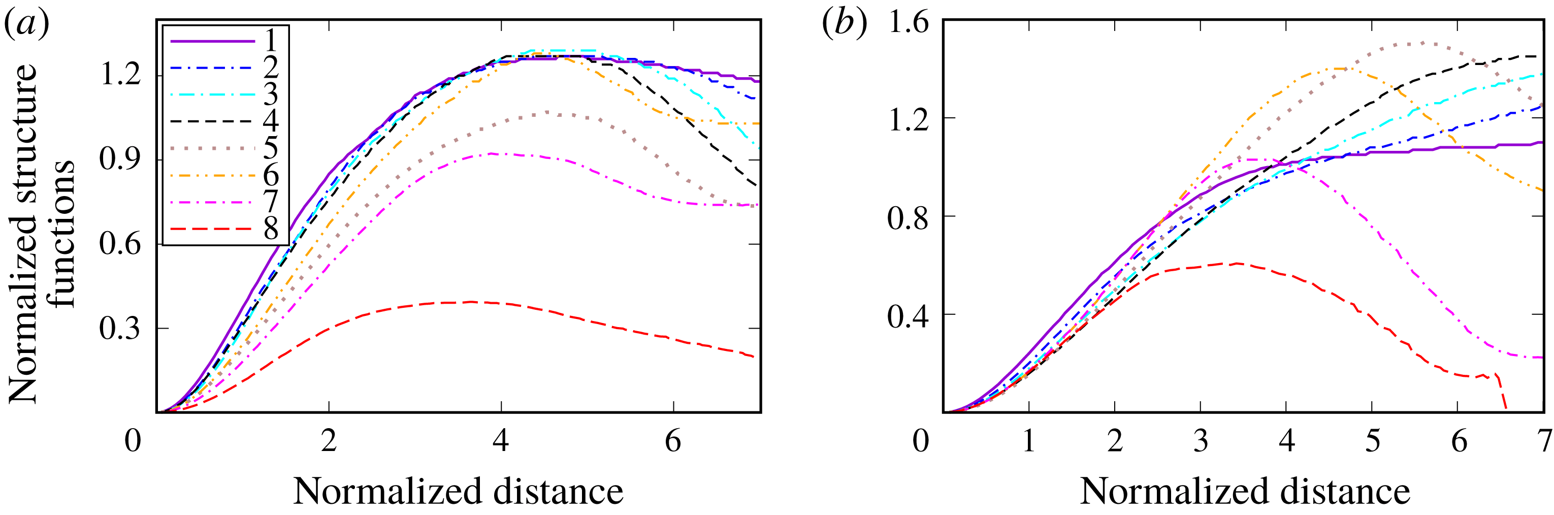
Such differences between cases H and L are even more pronounced if the SFs $D_{yz,L,uu}(x,r/\unicode[STIX]{x1D6FF}_{\unicode[STIX]{x1D716}})$ are ‘compensated’ by dividing them by reference SFs $D_{yz,L,uu}^{\ast }\equiv D_{yz,L,uu}(x=0.25~\text{mm},r/\unicode[STIX]{x1D6FF}_{\unicode[STIX]{x1D716}})$ , which are almost the same in cases H and L. Figure 12(b) (case L) shows that $D_{yz,L,uu}(x,r/\unicode[STIX]{x1D6FF}_{\unicode[STIX]{x1D716}})/D_{yz,L,uu}^{\ast }$ decreases with distance $x$ (or with $\langle c\rangle$ ) at small scales ( $r/\unicode[STIX]{x1D6FF}_{\unicode[STIX]{x1D716}}<4$ ). On the contrary, curves 5–8 in figure 12(a) (case H) show that $D_{yz,L,uu}(x,r/\unicode[STIX]{x1D6FF}_{\unicode[STIX]{x1D716}})/D_{yz,L,uu}^{\ast }$ increases with increasing $\langle c\rangle$ provided that $r/\unicode[STIX]{x1D6FF}_{\unicode[STIX]{x1D716}}<4$ . Moreover, local maxima of $D_{yz,L,uu}(x,r/\unicode[STIX]{x1D6FF}_{\unicode[STIX]{x1D716}})/D_{yz,L,uu}^{\ast }$ are observed at $r/\unicode[STIX]{x1D6FF}_{\unicode[STIX]{x1D716}}\approx 2.6$ and $\langle c\rangle (x^{\ast })\approx 0.5$ , see curve 7 in figure 12(a), or at $r/\unicode[STIX]{x1D6FF}_{\unicode[STIX]{x1D716}}\approx 4$ and $\langle c\rangle (x)\approx 0.75$ , see curve 8. Furthermore, $D_{yz,L,uu}[\langle c\rangle (x)\approx 0.75,r/\unicode[STIX]{x1D6FF}_{\unicode[STIX]{x1D716}}]/D_{yz,L,uu}^{\ast }$ is larger than unity if $r/\unicode[STIX]{x1D6FF}_{\unicode[STIX]{x1D716}}>1$ in case H. These results confirm that combustion-induced thermal expansion can substantially affect small-scale two-point velocity statistics even in the turbulent flow of constant-density unburned reactants.

Figure 12.

A ratio of the longitudinal reactant–reactant SFs $D_{yz,L,uu}(x,r/\unicode[STIX]{x1D6FF}_{\unicode[STIX]{x1D716}})$ to a reference SF $D_{yz,L,uu}(x=0.25~\text{mm},r/\unicode[STIX]{x1D6FF}_{\unicode[STIX]{x1D716}})$ . Legends are explained in caption to figure 10.

Figure 13.

A ratio of reactant–reactant SFs to reference SFs obtained at $x=0.25$  mm. 1 – Longitudinal SF $D_{yz,L,uu}$ for tangential velocities $v$ and  $w$ ; 2 – transverse SF $D_{xx,T,uu}$ for the axial velocity  $u$ ; 3 – transverse SF $D_{yz,L,uu}$ for tangential velocities $v$ and  $w$ , with $\boldsymbol{r}$ being equal to $\{0,0,r\}$ and $\{0,r,0\}$ , respectively; 4 – longitudinal SF $D_{xx,L,uu}$ for the axial velocity  $u$ , defined with (4.1); 5 – transverse SF for tangential velocities $v$ and  $w$ , with $\boldsymbol{r}$ being equal to $\{r,0,0\}$ , i.e. $x_{B}=x_{A}+r$ , $y_{B}=y_{A}$ , and $z_{B}=z_{A}$ .

Figure 13 shows another effect of this kind, i.e. differences between various compensated reactant–reactant SFs are substantially more pronounced at small scales ( $r/\unicode[STIX]{x1D6FF}_{\unicode[STIX]{x1D716}}<3$ ) in case H when compared to case L, thus, indicating that the influence of combustion-induced thermal expansion on the turbulence in unburned gas is highly anisotropic.

The influence of combustion on the incoming turbulent flow of constant-density reactants can also be evidenced using other methods. For instance, the present authors (Lipatnikov et al. Reference Lipatnikov, Chomiak, Sabelnikov, Nishiki and Hasegawa2015b ; Sabelnikov & Lipatnikov Reference Sabelnikov and Lipatnikov2017) analysed the same DNS data in order to compare the behaviour of small-scale turbulence characteristics (i) upstream of the mean flame brushes H and L, (ii) at the leading points of the flame brushes at various  $t$ and (iii) at the unburned flamelet edges within the flame brushes. For these purposes, first, the flame leading point $\boldsymbol{x}_{lp}(t)$ was found by selecting the single grid point with the lowest axial coordinate $x$ among all grid points characterized by $c(\boldsymbol{x},t)\geqslant 0.05$ at each instant  $t$ . Subsequently, quantities conditioned to this point were evaluated by averaging their values over a small square located on the leading transverse plane $x=x_{lp}(t)$ and centred around the leading point $\boldsymbol{x}_{lp}(t)$ . Second, due to the decay of incoming turbulence in the axial direction, quantities averaged over the leading transverse plane $x=x_{lp}(t)$ were considered to characterize turbulence upstream of the mean flame brush. Third, at each instant  $t$ , the unburned flamelet edge $x=x_{f}(y,z,t)$ , i.e. a 2-D surface within the mean flame brush, was found using the following two constraints; (i)  $c(x_{i},y_{j},z_{k},t)\geqslant 0.05$ if $x_{i}=x_{f}(y_{j},z_{k},t)$ , but (ii)  $c(x_{i},y_{j},z_{k},t)<0.05$ if $x_{i}<x_{f}(y_{j},z_{k},t)$ at the same $j$ and  $k$ . In other words, for each ray $\{\,j=\text{const.},k=\text{const.}\}$ (or $\{y=\text{const.},z=\text{const.}\}$ ) parallel to the $x$ -axis, a single axial coordinate $x_{i}=x_{f}(y_{j},z_{k},t)$ was determined so that $c(x,y_{j},z_{k},t)<0.05$ on the ray upstream of the unburned flamelet edge, but $c(x_{i},y_{j},z_{k},t)\geqslant 0.05$ at the boundary. Then, the value of a considered quantity was averaged over the entire 2-D surface of the unburned flamelet edge $x_{f}(y,z,t)$ at different instants, i.e. over all $1\leqslant j\leqslant 128$ and $1\leqslant k\leqslant 128$ and over $t_{II}\leqslant t\leqslant t_{III}$ . Thus, (i) characteristics of the incoming turbulence were averaged over the leading transverse plane $x=x_{lp}(t)$ upstream of the mean flame brush, (ii) characteristics of the leading point were averaged in its vicinity and (iii) characteristics of the unburned flamelet edge were averaged over a 2-D surface within the mean flame brush.

Three quantities, i.e. enstrophy $\unicode[STIX]{x1D714}^{2}=(\unicode[STIX]{x1D735}\times \boldsymbol{u})^{2}$ , total strain $S^{2}=\unicode[STIX]{x1D61A}_{ij}\unicode[STIX]{x1D61A}_{ij}$ and the $Q$ -criterion (Tsinober Reference Tsinober2009)

(4.2) $$\begin{eqnarray}\displaystyle Q={\textstyle \frac{1}{4}}\unicode[STIX]{x1D714}^{2}-{\textstyle \frac{1}{2}}S^{2}, & & \displaystyle\end{eqnarray}$$

were studied to explore the influence of combustion-induced thermal expansion on small-scale turbulence by comparing their values averaged in the incoming turbulence with their values conditioned to either the leading point or to the unburned flamelet edge.

Figure 14.

(a) $Q$ criterion (solid lines), total strain $S^{2}/2$ (dashed lines) and enstrophy $\unicode[STIX]{x1D714}^{2}/4$ (dotted lines), averaged in the vicinity of the leading points $x_{lp}(t)$ (red and orange lines in cases H and L, respectively) and over leading planes $x=x_{lp}(t)$ (blue and violet lines in cases H and L, respectively). (b) Probabilities of $Q>0$ (solid lines) and $Q<0$ (dashed lines), conditioned to unburned flamelet edge, i.e. $c(\boldsymbol{x},t)\approx 0.05$ .

Figure 14(a) shows that the behaviour of $\unicode[STIX]{x1D714}^{2}$ , $S^{2}$ or $Q$ averaged over the leading plane, i.e. in the incoming turbulent flow, is similar in cases H and L, cf. blue and violet lines. In both cases, the magnitudes of $\unicode[STIX]{x1D714}^{2}/4$ and $S^{2}/2$ are much larger than the magnitude of  $Q$ , which is predominantly negative. Moreover, in case L, the behaviour of $Q$ averaged in the vicinity of the leading point is similar to the behaviour of $Q$ averaged over the leading plane, cf. solid orange and violet lines. On the contrary, in case H characterized by a significantly larger density ratio, the behaviour of  $Q$ , $\unicode[STIX]{x1D714}^{2}$ or $S^{2}$ averaged in the vicinity of the leading point differs significantly from the behaviour of  $Q$ , $\unicode[STIX]{x1D714}^{2}$ or  $S^{2}$ , respectively, averaged over the leading plane, cf. red and blue lines. In particular, the former $Q$ is always negative, see red solid line, thus, indicating a substantial influence of combustion-induced thermal expansion on small-scale turbulent structure in the unburned constant-density reactants. The negative values of $Q$ averaged in the vicinity of the leading point imply that the potential flow perturbations caused by the thermal expansion overwhelm the rotational perturbations. In other words, the flow in the vicinity of the leading point appears to be significantly affected by pressure perturbations generated within flamelets.

Figure 15.

Typical 2-D images of the sign of the $Q$ -criterion in cases (a) H and (b) L. Spatial regions characterized by $Q>0$ and $Q<0$ are shown in grey and white, respectively. Left and right solid lines show surfaces of $c(\boldsymbol{x},t)\approx 0.01$ and $c(\boldsymbol{x},t)\approx 0.5$ , respectively. Spatial $x$ and $y$ coordinates are reported in mm, $z=2$  mm.

Figure 14(b) reports probabilities of positive (solid lines) and negative (dashed lines) $Q$ at the unburned flamelet edge $x=x_{f}(y,z,t)$ . In case L, the probabilities of $Q<0$ and $Q>0$ are comparable. On the contrary, values of $Q$ calculated at the unburned flamelet edge are negative in case H almost always, indicating a substantial influence of combustion-induced thermal expansion on small-scale turbulent structures in the unburned constant-density reactants. Again, the negative values of $Q$ evaluated at the unburned flamelet edge imply that the flow upstream of the flamelets is significantly affected by pressure perturbations generated within the flamelets.

Typical 2-D images of the sign of the $Q$ -criterion, plotted in figure 15, also indicate that $Q<0$ in the vicinity of the flamelets in case H, but $Q$ can change sign within the flamelets in case L.

Finally, it is worth noting that while figures 14 and 15 may appear to show the influence of combustion on the incoming turbulence in a clearer manner when compared to figures 10–13, the latter results convey additional information. In particular, contrary to the conditioned SFs, values of $\unicode[STIX]{x1D714}^{2}$ , $S^{2}$ or $Q$ do not allow us to compare the magnitudes of the discussed effects at different length scales.

4.4 Turbulence in heat-release zones

SFs conditioned to HRZs, introduced in § 2.2, offer an opportunity to show the influence of combustion-induced thermal expansion on two-point statistics of the turbulent velocity field within such zones. If solely events such that the entire segment $[\text{A},\text{B}]$ is within the HRZ are selected, then, the probability of these events is low and decreases rapidly with distance $r$ between the considered points A and B, see figure 16. Accordingly, statistically solid results can only be obtained at sufficiently small  $r$ . Nevertheless, the method does offer an opportunity to study behaviour of small-scale velocity differences in HRZs.

Figure 16.

Probabilities of finding the entire segment $[\text{A},\text{B}]$ within HRZs ( $0.75<c(\boldsymbol{x},t)<0.95$ ), obtained at three different $\langle c\rangle (x)$ specified in the legend, versus the normalized segment length $r/\unicode[STIX]{x1D6FF}_{\unicode[STIX]{x1D716}}$ . Red and blue lines show results obtained in cases H and L, respectively.

Figure 17.

Transverse SFs $D_{xx,T,ww}[\langle c\rangle (x),r/\unicode[STIX]{x1D6FF}_{\unicode[STIX]{x1D716}}]$ (black lines) and $D_{yz,T,ww}[\langle c\rangle (x),r/\unicode[STIX]{x1D6FF}_{\unicode[STIX]{x1D716}}]$ (red lines) conditioned to HRZs ( $0.75<c(\boldsymbol{x},t)<0.95$ ) at three different $\langle c\rangle (x)$ specified in the legends. The SFs are normalized with $u^{\prime 2}$ and $0.5(v^{\prime 2}+w^{\prime 2})$ , respectively, conditioned to the same zone at the same $\langle c\rangle$ . (a) case H, (b) case L.

For instance, figure 17 indicates that the transverse SFs $D_{xx,T,ww}[\langle c\rangle (x),r/\unicode[STIX]{x1D6FF}_{\unicode[STIX]{x1D716}}]$ and $D_{yz,T,ww}[\langle c\rangle (x),r/\unicode[STIX]{x1D6FF}_{\unicode[STIX]{x1D716}}]$ differ significantly from one another at low $r/\unicode[STIX]{x1D6FF}_{\unicode[STIX]{x1D716}}$ in case H, but exhibit similar dependencies on $r/\unicode[STIX]{x1D6FF}_{\unicode[STIX]{x1D716}}$ in case L. In particular, at low $r/\unicode[STIX]{x1D6FF}_{\unicode[STIX]{x1D716}}$ , the shape of the $D_{xx,T,ww}(r/\unicode[STIX]{x1D6FF}_{\unicode[STIX]{x1D716}})$ -curves in figure 17(a) differs significantly from the shape of the other curves.

The observed increase in $D_{xx,T,ww}[\langle c\rangle (x),r/\unicode[STIX]{x1D6FF}_{\unicode[STIX]{x1D716}}]$ at low $r/\unicode[STIX]{x1D6FF}_{\unicode[STIX]{x1D716}}$ in case H may be associated with vorticity generation by baroclinic torque. Indeed, first, the present DNS data show that the components $\unicode[STIX]{x1D714}_{y}$ and $\unicode[STIX]{x1D714}_{z}$ of the vorticity vector $\unicode[STIX]{x1D735}\times \boldsymbol{u}$ are increased by baroclinic torque within the H-flame brush, whereas $\unicode[STIX]{x1D714}_{x}$ in case H and all three components of the vorticity vector in case L are decreased with increasing $\langle c\rangle$ due to dilatation (Lipatnikov et al. Reference Lipatnikov, Nishiki and Hasegawa2014, figure 2b). Second, variations in the axial velocity $u$ in the transverse directions $y$ and  $z$ , i.e. $D_{xx,T,ww}$ , contribute to $\unicode[STIX]{x1D714}_{z}$ and $\unicode[STIX]{x1D714}_{y}$ , respectively, whereas variations in the tangential velocities $v$ and $w$ in the transverse directions $z$ and  $y$ , respectively, i.e. $D_{yz,T,ww}$ , contribute to  $\unicode[STIX]{x1D714}_{x}$ . Consequently, (i) results plotted in figure 17(a) are in line with different behaviours of $\unicode[STIX]{x1D714}_{y}$ or $\unicode[STIX]{x1D714}_{z}$ (an increase with $\langle c\rangle$ ) and $\unicode[STIX]{x1D714}_{x}$ (a decrease with $\langle c\rangle$ ), reported in case H by Lipatnikov et al. (Reference Lipatnikov, Nishiki and Hasegawa2014, figure 2b), and (ii) results plotted in figure 17(b) are in line with similar behaviours of  $\unicode[STIX]{x1D714}_{x}$ , $\unicode[STIX]{x1D714}_{y}$ and  $\unicode[STIX]{x1D714}_{z}$ , reported in case L by Lipatnikov et al. (Reference Lipatnikov, Nishiki and Hasegawa2014, figure 2b). Accordingly, not only viscous dissipation and dilatation, but also baroclinic torque may significantly affect small-scale turbulent eddies in flamelet preheat zones and the net effect (dissipation or generation of such eddies) depends on the conditions and is highly anisotropic. The conditioned SFs introduced in the present work appear to be an appropriate tool for exploring the competition of such mechanisms by analysing experimental or DNS data obtained under various conditions.