2. Related work

Researchers explored various measures to combat EDoS attacks in cloud computing. Baig et al. [Reference Baig, Sait and Binbeshr3] proposed a mitigation technique to deal with EDoS attacks based on a rate limit technique to prevent malicious requests from being served before passing through investigative tests. Al-Haidari et al. [Reference Al-Haidari, Sqalli and Salah1] studied the impact of EDoS attacks on a single class of cloud computing services by formulating a queuing model. The authors in [Reference Al-Haidari, Sqalli and Salah1] obtained certain performance metrics such as end-to-end response time, mean computing utilization, throughput and the cost incurred due to the attacks. Monge et al. [Reference Monge, Vidal and Perez19] identified two types of EDoS threats, namely workload-based EDoS attacks and instantiation-based EDoS attacks. The authors in [Reference Monge, Vidal and Perez19] then formulated an entropy-based EDoS detection approach to mitigate the threats in self-organizing networks. Shawahna et al. [Reference Shawahna, Abu-Amara, Mahmoud and Osais23] presented a novel approach for mitigating EDoS attacks which is referred to as EDoS-ttack efense hell. The authors in [Reference Shawahna, Abu-Amara, Mahmoud and Osais23] used $M/M/1$ queuing model in their approach to evaluate the cost incurred, throughput and CPU utilization in the presence of EDoS attacks. It has been reported that not only the cloud adopters (end users) but also cloud service providers can be affected by the EDoS attacks. One such attack is discussed by Ficco [Reference Ficco9] in which the attackers try to exploit the elasticity and multi-tenancy of the cloud infrastructure to carry out fraudulent energy consumption attacks against cloud service providers. Wang et al. [Reference Wang, Xi, Li and Chen25] proved that EDoS attacks can be launched easily by abusing public third-party services. They also indicated that a good cooperation between the cloud consumers and the public third parties is needed to mitigate the attacks.

Dinh et al. [Reference Dinh and Park6] dealt with a stealthy EDoS attack based on multivariate time series and proposed a scheme named R-EDoS to detect anomaly traffic due to EDoS attacks in SDN-based cloud. Shah et al. [Reference Shah, Khan and Ahmed22] proposed a mitigation technique called Internet Control Messaging Protocol attack detection for flooding attacks which can lead to an EDoS attack. In our recent work [Reference Lalropuia and Khaitan (nee Gupta)17], we have dealt with the availability and reliability issues of cloud computing under EDoS attack based on a semi-Markov process. However, in this paper [Reference Lalropuia and Khaitan (nee Gupta)17] we have not taken into account the different strategies that the malicious users as well as the defender can adopt in the event of an EDoS attack. Chowdhury et al. [Reference Chowdhury, Idna Idris, Mat Kiah and Manazir Ahsan5] proposed a game theoretical model for mitigating EDoS attacks. The authors in [Reference Chowdhury, Idna Idris, Mat Kiah and Manazir Ahsan5] employ a static game of complete information to capture the interplay between the attacker and the system defender. However, in reality, the types of incoming traffic are not completely known to the system defender and so is the behavior of the attackers. Furthermore, the nature of many strategic interactions is better captured by a dynamic environment in comparison to a static environment [Reference Etesami and Basar8]. Therefore, these shortcomings of the existing literature motivated us to employ a signaling game that is a dynamic game of incomplete information to mitigate the EDoS attacks in cloud computing. In contrast to a static Bayesian game where the players simultaneously choose the actions without knowing the actions chosen by the other players [Reference Lalropuia and Gupta16], a signaling game is a dynamic Bayesian game in which the sender (the attacker in the context of this paper) first sends a service request and the receiver (the defender in this paper) takes necessary actions after observing the sender's action.

The main contributions of this paper are summarized as below:

• • A novel game theoretic model is proposed to address the EDoS attacks in cloud computing using a signaling game which is a type of dynamic Bayesian game.

• • Based on the proposed signaling game model, the behavioural traits of the attacker and the defender are predicted by computing the perfect Bayesian Nash equilibrium (PBE). Various types of PBE such as the pooling PBE, separating PBE and mixed strategy PBE are obtained corresponding to the best defense strategies against the attacks.

• • Numerical illustrations are presented which give insights into how different expected payoffs and mixed strategy equilibrium probability of the game model are affected by the traffic dropping probability.

The rest of the paper is organized as follows: Section 3 covers the proposed game model. The associated expected payoffs are derived in Section 4. In Section 5, the Bayesian Nash equilibrium analysis of the proposed game model is discussed. The numerical results and illustrations are presented in Section 6 and the conclusion follows in Section 7.

3. Proposed game model

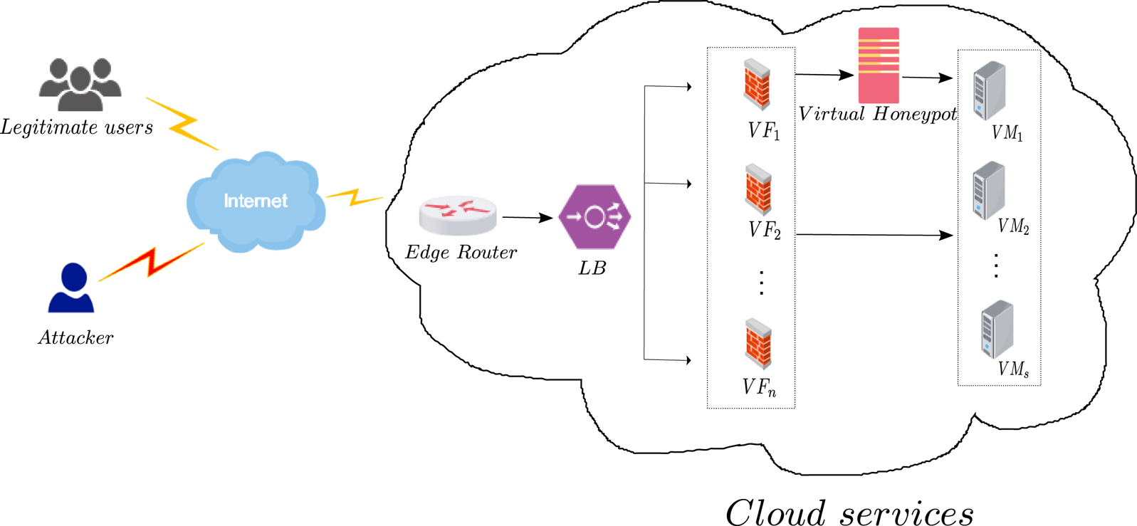
In this section, we propose a signaling game model to address the EDoS attacks in cloud computing and, for this, we consider a cloud service of IaaS type. To develop the game model, we first discuss about the main components of the cloud architecture which consists of an Edge Router, a Load Balancer (LB), Virtual Firewall (VF), a Virtual Honeypot (VH) and Virtual Machine (VM) instances. The service requests are served by the VMs as shown in Figure 1. The edge router acts as a gateway for both legitimate and malicious traffic. The LB is responsible for a uniform distribution of the incoming traffic among the $n$ VFs. The current utilization of the cloud system and the auto-scaling thresholds are also monitored by the LB. VFs are employed to filter the malicious traffic based on some predetermined thresholds of the incoming traffic. The suspicious traffic as identified by the VF are not directly dropped by the VF, it instead redirects them to the VH for further examination, and then the malicious traffic is dropped by the honeypot manager [Reference Biedermann, Mink and Katzenbeisser4].

Figure 1.

Network topology under consideration for the proposed game model.

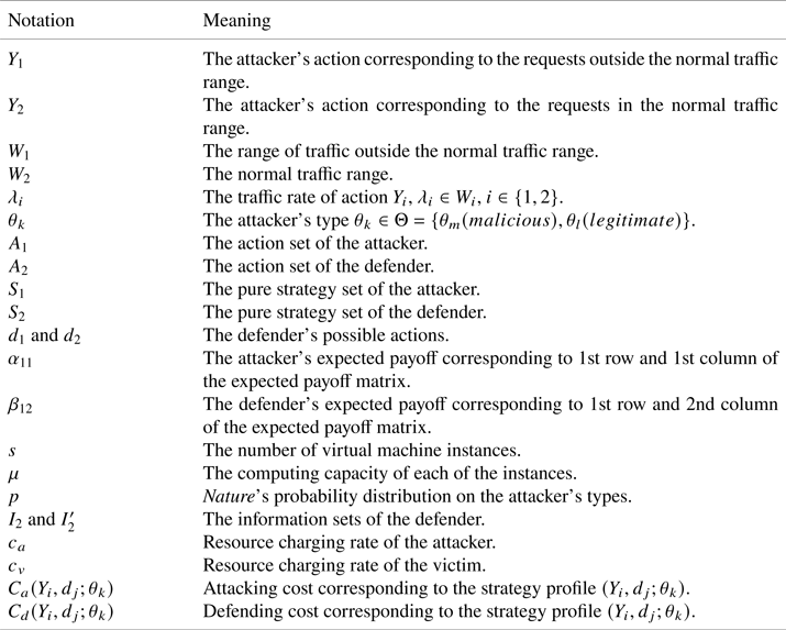
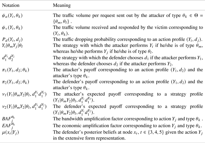
In the case of an EDoS attack against the cloud service under consideration, we capture the interactions between the malicious user (i.e., the attacker) and the defender (i.e., the VFs) with the help of a signaling game in which the two players are the attacker and the defender. The attacker sends a service request and then the defender (i.e., the VFs) responds to it after observing the attacker's action (i.e., the types of the traffic). To discuss the proposed game model in more detail, we introduce a list of notations and symbols given in Tables 1 and 2.

Table 1.

Notations used in the proposed game model

Table 2.

Some more notations used in the proposed game model

We assume that the attacker can act as either malicious or legitimate user, that is, the attacker has two types: malicious ($\theta _m$) and legitimate ($\theta _l$), and the legitimate type attacker can be identified with a legitimate (or regular) user. In addition, we consider that the attacker can launch EDoS attacks in two ways represented by actions $Y_1$ and $Y_2$ which are described below:

Action $Y_1$: Suppose the legitimate users gain access to the cloud services with traffic rate $\lambda _2$ in some normal request range. Then, we let the action $Y_1$ denotes the action of the attacker when he/she performs EDoS attacks by sending malicious requests outside the normal (legitimate) traffic range. In this case, the malicious traffic of rate $\lambda _1$ (request per second) is sent with the traffic volume $\psi _a(Y_1,\theta _m)$ per request. Let

$$W_1 = \{\lambda_1 \in \mathbb{Z^{+}}: 1 \leq \lambda_1 \leq \eta - 1\} \cup \{\lambda_1 \in \mathbb{Z^{+}}: \rho \leq \lambda_1 < \infty \}.$$

Here, $\mathbb {Z^{+}}$ denotes the set of positive integers, $\eta$ and $\rho \in \mathbb {Z^{+}}$. If the normal (legitimate) traffic range is denoted by

$$W_2 = \{\lambda_2 \in \mathbb{Z^{+}}: \eta \leq \lambda_2 \leq \rho - 1\},$$

then $W_1$ is the sending range consisting of all the traffic below normal traffic (which corresponds to extremely stealthy attacks) and above normal traffic (which corresponds to typical EDoS attacks including brute force attack [Reference Ficco9]). Thus, we have $\lambda _1 \in W_1$, $\mathbb {Z^{+}} = W_1 \cup W_2$ and $W_1\cap W_2 = \phi$, where $\phi$ denotes the empty set.

Action $Y_2$: The action $Y_2$ denotes the action of the attacker when he/she launches EDoS attacks by sending malicious service requests with rate $\lambda _2$ and traffic volume $\psi _a(Y_2,\theta _m)$ per request in the normal traffic range $W_2$ (i.e., $\lambda _2 \in W_2$). In this case, the attacker tries to evade detection by pretending to be a legitimate user. The attack in this case is stealthy and hard to detect as the legitimate traffic are blended with the malicious traffic in the same request sending range $W_2$. In addition, the legitimate type attacker gains access to the service with traffic rate $\lambda _2 \in W_2$ and traffic volume $\psi _a(Y_2,\theta _l)$ per request, however, he/she does not perform any attack.

To respond to the malicious activities VFs along with a honeypot are incorporated in the proposed game model, that is, the VFs act as the defender against the attacker. The VF predetermines threshold parameters for the traffic rate and traffic volume as ($\lambda ^{*}, v^{*}$) such that if the traffic rate $\lambda \leq \lambda ^{*}$ and the traffic volume $\psi _a(Y_i,\theta _k) \leq v^{*}$, then the traffic is accepted; otherwise, there are two possible actions for the VF as discussed below:

Action $d_1$ : The action $d_1$ denotes the action when the VF redirects traffic to the honeypot for further investigation. This traffic with rate $\lambda _i$ and volume $\psi _a(Y_i,\theta _k)$ is caused by the attacker of type $\theta _k$ when he/she performs the action $Y_i$. Upon examining the traffic, the honeypot manager drops the traffic with probability $P_d(Y_i,d_j)$ or accepts them with probability $1 - P_d(Y_i,d_j)$ for $j=1$ thus allowing access to the service. Here, $i\in \{1,2\}$, $\theta _k\in \{\theta _m, \theta _l\}$.

Action $d_2$: The action $d_2$ denotes the action in which the VF does not redirect traffic to the honeypot, it instead directly allows the traffic to pass through it, thereby allowing access to the service. Hence, the traffic dropping probability in this case is zero, that is, $P_d(Y_i,d_j) = 0$ for $j = 2$, $i\in \{1,2\}$.

As stated above, the attacker has two types: malicious and legitimate. On the other hand, the system defender (VF) is assumed to have only one type (i.e., regular). Thus, the interplay between the attacker and the defender can be modeled as a dynamic game of incomplete information such as a signaling game. In a signaling game, the sender (the attacker in this paper) first sends a signal and the receiver (the defender) observes the sender's action. Then, the defender takes actions based on the observed action of the attacker.

Now, we describe the interactions between the attacker and the defender based on a signaling game. The proposed signaling game is denoted by $\Gamma$ and consists of the following components:

• • The set of players, $\chi = \{Attacker,\ Defender\}$.

• • The attacker's action set, $A_1 = \{Y_1,\ Y_2\}$.

• • The attacker's type set, $\Theta = \{malicious\ (\theta _m),\ legitimate\ (\theta _l)\}$.

• • Nature's probability distribution on the attacker's type, $\zeta :\Theta \rightarrow [0,1]$, such that $\zeta (\theta _m) = p$ and $\zeta (\theta _l)= 1 - p$. Here, Nature can be considered as a non-strategic player with stochastic strategies.

• • The defender's action set $A_2 = \{d_1, d_2\}$, and the defender's type is regular and is common knowledge among the players.

• • The action space, $A = A_1 \times A_2$.

• • The pure strategy set of the attacker, $S_1 = \{Y_1 |_{\theta _m} Y_2|_{\theta _l},\ Y_2|_{\theta _m} Y_2|_{\theta _l}\}$, where $Y_1 |_{\theta _m} Y_2|_{\theta _l}$ denotes the strategy with which the attacker performs action $Y_1$ if he/she is malicious ($\theta _m$), whereas he/she takes the action $Y_2$ if he/she is legitimate ($\theta _l$). And $Y_2|_{\theta _m} Y_2|_{\theta _l}$ is the strategy with which the attacker performs the action $Y_2$ if his/her type is malicious and he/she performs the action $Y_2$ if his/her type is legitimate.

• • The pure strategy set of the defender, $S_2 = \{d_1^{Y_1} d_1^{Y_2},~ d_1^{Y_1} d_2^{Y_2},\ d_2^{Y_1} d_1^{Y_2},\ d_2^{Y_1} d_2^{Y_2}\}$, where $d_1^{Y_1} d_1^{Y_2}$ is the strategy with which the defender takes the action $d_1$ if the attacker performs the action $Y_1$, whereas the defender takes the action $d_1$ if the attacker performs the action $Y_2$ and so on.

• • The strategy space of the players, $S = S_1 \times S_2$.

• • The payoff function of player $i \in \chi$, $\pi _i : A \times \Theta \rightarrow \mathbb {R}$, where $\mathbb {R}$ is the set of real numbers and $\pi _i(Y_j,d_k; \theta )$ is the payoff corresponding to the profile of action $(Y_j, d_k)$, $j, k \in \{1,2\}$ if the attacker is of type $\theta \in \Theta$. For simplicity, we use $\pi _1$ and $\pi _2$ to denote the payoffs of the attacker and the defender, respectively.

• • The expected payoff function of player $i$, $\nu _i: S \rightarrow \Omega$, where

  $$\Omega = \{p\pi_i(Y_j,d_k;\theta_m) + (1-p) \pi_i(Y_2, d_s;\theta_l) \,:\, j, k, s \in \{1,2\},\ 0\leq p \leq 1 \}.$$

To specify the payoffs of the two players in the proposed game model discussed above, we first present some definitions related to the EDoS attacks. EDoS attack is a type of amplification attack where the attackers make use of a small amount of resource to make the victim suffer relatively high resource stress [Reference Wang, Xi, Li and Chen25]. Examples of amplification attacks include DNS amplification attacks [7] and smurf attacks [Reference Kumar15]. In EDoS amplification attack, we consider the amplification based on bandwidth as defined below:

Definition 1 [Reference Kumar15,Reference Wang, Xi, Li and Chen25]

Bandwidth amplification factor $(\textit{BAF}_j^{\theta _k})$ corresponding to the action $Y_j$ and the attacker's type $\theta _k$ is defined as

(1)\begin{equation} \textit{BAF}_j^{\theta_k} = \frac{\psi_{v}(Y_j,\theta_k)}{\psi_{a}(Y_j,\theta_k)} \end{equation}

where $\psi _a(Y_j, \theta _k)$ denotes the traffic volume sent out per request when the attacker of type $\theta _k \in \Theta$ takes the action $Y_j$, and $\psi _v(Y_j, \theta _k)$ is the corresponding traffic volume received and responded by the victim.

Given the definition of $BAF$, a convenient measure to assess the economic burden imposed by the attacks is economic amplification factor (EAF). It is defined as:

Definition 2 [Reference Wang, Xi, Li and Chen25]

Economic amplification factor $(\textit{EAF}_j^{\theta _k})$ corresponding to the action $Y_j$ and the attacker's type $\theta _k$ is defined as

(2)\begin{equation} \textit{EAF}_j^{\theta_k} = \frac{c_v\psi_{v}(Y_j,\theta_k)}{c_a\psi_{a}(Y_j,\theta_k)} \end{equation}

or

(3)\begin{equation} \textit{EAF}_j^{\theta_k} = \frac{c_v}{c_a} \textit{BAF}_j^{\theta_k} \end{equation}

where $c_a$ and $c_v$ are the resource charging rates for the attacker and the victim, respectively.

In an amplification attack, if the attacker's type is malicious ($\theta _m$), the BAF and hence the EAF is greater than $1$, that is,

(4)\begin{equation} \textit{EAF}_j^{\theta_m} = \frac{c_v\psi_{v}(Y_j,\theta_m)}{c_a\psi_{a}(Y_j,\theta_m)} > 1,\quad \text{for}\ j = 1,2. \end{equation}

Recall that the malicious type attacker sends requests with rate $\lambda _j$ when he/she performs the action $Y_j$, $j = 1, 2$. For $\lambda _1 > \lambda _2$, the corresponding BAF and hence the EAF due to $\lambda _1$ is greater than that of the amplification produced by $\lambda _2$, that is, $\lambda _1 > \lambda _2$ implies

(5)\begin{equation} \textit{EAF}_1^{\theta_m} > \textit{EAF}_2^{\theta_m}. \end{equation}

As described previously, $P_d(Y_i,d_j)$ is used to denote the dropping probability of the traffic with rate $\lambda _i$ when the action $Y_i$ is implemented and the defender responds to the attacker's action by the action $d_j$. Thus, $1 - P_d(Y_i,d_j)$ is the probability of allowing the traffic with rate $\lambda _i$ sent out by the attacker. With the action $d_2$, the defender admits all the traffic, thereby allowing them to gain access to the cloud services. Therefore, the dropping probabilities of all incoming traffic are zero, that is,

(6)\begin{equation} P_d(Y_i,d_2) = 0,\quad \text{for}\ i = 1, 2. \end{equation}

On the other hand, if the defender takes the action $d_1$, there exists a positive probability with which the incoming traffic is dropped by the $\textit {VH}$ manager. This can be expressed as

(7)\begin{equation} P_d(Y_i,d_1) > 0,\quad \text{for}\ i = 1, 2. \end{equation}

In the proposed model, we assume that both the legitimate and malicious traffic arrive according to Poisson processes with rate $\lambda _l$ and $\lambda _m$, respectively [Reference Al-Haidari, Sqalli and Salah1,Reference Shawahna, Abu-Amara, Mahmoud and Osais23]. It is evident that merging two Poisson processes results in a Poisson process [Reference Ross20], hence the aggregate traffic follows Poisson process with rate $\lambda = \lambda _l + \lambda _m$. In addition, we assume that each of the VM instances have the same computing power capacity which is captured by the exponential distribution with rate $\mu$. Therefore, the VM instances can be modeled as an $M/M/s$ queuing model [Reference Gross, Shortle, Thompson and Harris13], and therefore, the mean computing utilization $U$ is given by [Reference Al-Haidari, Sqalli and Salah1]

(8)\begin{equation} U = \frac{\lambda}{s\mu}=\frac{\lambda_l + \lambda_m}{s\mu}, \end{equation}

and the mean utilization incurred by the attacker is equal to ${\lambda _m}/{s\mu }$.

A rational attacker will try to optimize his/her payoffs by maximizing both the CPU utilization incurred due to $\lambda _i$, that is, $U_i = {\lambda _i}/{s\mu }$ and the EAF, $\textit{EAF}_i^{\theta _k}$ by performing the action $Y_i$.

Let $C_a(Y_i, d_j; \theta _k) \geq 0$ denote the attacking cost incurred due to a profile of strategy $(Y_i, d_j;\theta _k)$. That is, $C_a(Y_i, d_j; \theta _k)$ is the attacking cost incurred when the attacker of type $\theta _k$ performs the action $Y_i$ and the defender takes the action $d_j$. Since the attacker is trying to maximize both the CPU utilization and the EAF with respect to the attacking cost, the attacker's payoff $\pi _1(Y_i,d_j;\theta _k)$ corresponding to the action profile $(Y_i,d_j)$ if he/she is of type $\theta _k$ and the traffic dropping probability $P_d(Y_i, d_j)$ can be formulated as (for $i = 1,2$; $j = 1,2$; and $\theta _k \in \Theta$):

(9)\begin{equation} \pi_1(Y_i,d_j;\theta_k) = \left(\frac{\lambda_i}{s\mu} + \textit{EAF}_i^{\theta_k}\right)\{1 - P_d(Y_i,d_j)\} - C_a(Y_i, d_j; \theta_k). \end{equation}

Note that since the legitimate type attacker does not perform the action $Y_1$, therefore $\pi _1(Y_1,d_j;\theta _l)$ is not included in Eq. (9).

Moreover, the defender will try to maximize its payoff by spending the defending cost $C_d(Y_i, d_j;\theta _k) \geq 0$ due to $d_j$, $j\in \{1,2\}$ to respond to the action $Y_i$ performed by the attacker of type $\theta _k$. That is, $C_d(Y_i, d_j;\theta _k)$ is the defending cost corresponding to the strategy profile $(Y_i, d_j; \theta _k)$. This maximization is equivalent to minimizing the attacker's payoff (excluding the attacking cost) with respect to the defending cost 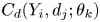$C_d(Y_i, d_j; \theta _k)$. Therefore, the defender's payoff $\pi _2(Y_i,d_j;\theta _k)$ corresponding to the action profile $(Y_i, d_j)$, the traffic dropping probability $P_d(Y_i, d_j)$ and the attacker's type $\theta _k \in \Theta$ can be written as

(10)\begin{equation} \pi_2(Y_i,d_j;\theta_k) ={-}\left(\frac{\lambda_i}{s\mu} + \textit{EAF}_i^{\theta_k}\right) \{1- P_d(Y_i,d_j)\} - C_d(Y_i, d_j;\theta_k). \end{equation}

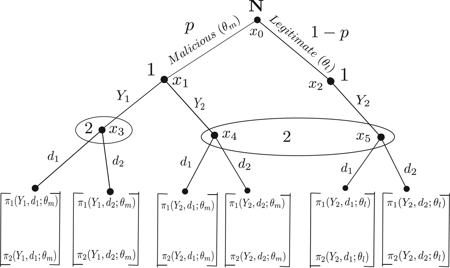
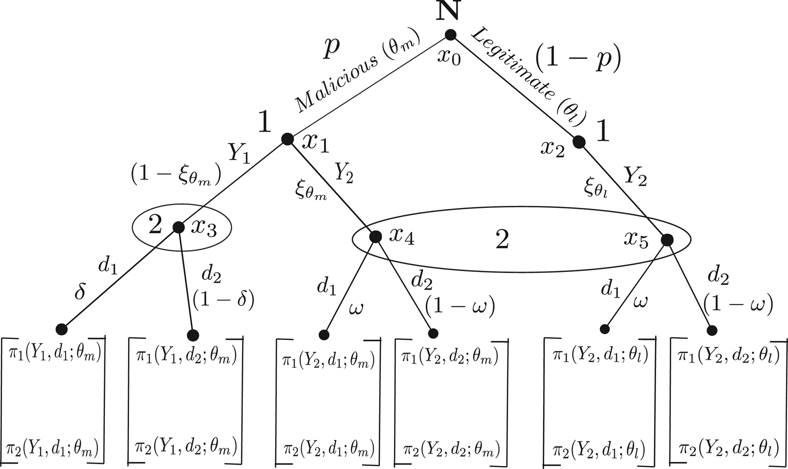
It should be noted that $C_d(Y_i, d_2;\theta _k) = 0$ for each $i \in \{1,2\}$ and $\theta _k \in \Theta$. The extensive form representation of the proposed game model is shown in Figure 2. The defender has two information sets $I_2 = \{x_3\}$ and $I^{\prime }_2 = \{x_4, x_5\}$ as shown in Figure 2. In the information set $I_2$, the defender knows that the action $Y_1$ is performed by an attacker whose type is malicious ($\theta _m$) with probability $1$. On the other hand, in the information set $I^{\prime }_2$, the defender knows that the action $Y_2$ is performed by a user whose type is either malicious ($\theta _m$) with probability $p$ or legitimate ($\theta _l$) with probability $1 - p$. These prior probabilities are determined by Nature.

Figure 2.

Extensive form representation of the signaling game.

4. Expected payoffs

In this section, we compute the expected payoffs of the two players. Let $\alpha _{11}$ denote the expected payoff of the attacker corresponding to the profile of strategy $(Y_1|_{\theta _m}Y_2|_{\theta _l}, d_1^{Y_1}d_1^{Y_2})$. From Figure 2, it can be computed as:

$$\alpha_{11} = \nu_1(Y_1|_{\theta_m}Y_2|_{\theta_l},d_1^{Y_1}d_1^{Y_2}) = p\pi_1(Y_1, d_1;\theta_m) + (1-p)\pi_1(Y_2,d_1;\theta_l).$$

Similarly, the expected payoff corresponding to the other strategy profiles can be calculated and are given in the following expected payoff matrix:

Expected payoff matrix 1

\begin{align*}\begin{matrix} & \begin{matrix}d_1^{Y_1}d_1^{Y_2} & & d_1^{Y_1}d_2^{Y_2} & & & d_2^{Y_1}d_1^{Y_2} & & & d_2^{Y_1}d_2^{Y_2}\end{matrix} \\ \begin{matrix}Y_1|_{\theta_m}Y_2|_{\theta_l}\\Y_2|_{\theta_m}Y_2|_{\theta_l}\end{matrix} & \begin{bmatrix}(\alpha_{11}\ \beta_{11}) & (\alpha_{12}, \ \beta_{12}) & (\alpha_{13}, \ \beta_{13}) & (\alpha_{14}, \ \beta_{14})\\ (\alpha_{21},\ \beta_{21}) & (\alpha_{22}, \ \beta_{22}) & (\alpha_{23},\ \beta_{23}) & (\alpha_{24},\ \beta_{24}) \end{bmatrix} \end{matrix}\end{align*}

where $\beta _{11} = \nu _2(Y_1|_{\theta _m}Y_2|_{\theta _l},d_1^{Y_1}d_1^{Y_2}) = p\pi _2(Y_1, d_1;\theta _m) + (1-p)\pi _2(Y_2,d_1;\theta _l)$ is the defender's expected payoff corresponding to the strategy profile $(Y_1|_{\theta _m}Y_2|_{\theta _l},d_1^{Y_1}d_1^{Y_2})$.

In addition, we have the following expected payoffs:

\begin{align*} \alpha_{12} & = \nu_1(Y_1|_{\theta_m}Y_2|_{\theta_l},d_1^{Y_1}d_2^{Y_2}) = p\pi_1(Y_1, d_1;\theta_m) + (1-p)\pi_1(Y_2,d_2;\theta_l)\\ \beta_{12} & = \nu_2(Y_1|_{\theta_m}Y_2|_{\theta_l},d_1^{Y_1}d_2^{Y_2}) = p\pi_2(Y_1, d_1;\theta_m) + (1-p)\pi_2(Y_2,d_2;\theta_l) \end{align*}

Similarly, the other payoffs can be obtained and the complete list of the elements of the payoff matrix is given in the Appendix.

5. Bayesian Nash equilibrium (BNE) analysis

It is shown in Figure 2 that the defender has two information sets denoted by $I_2 = \{x_3\}$ and $I^{\prime }_2 = \{x_4,x_5\}$.

• • Let $\mu (x_3\,|\,Y_1)$ denote the defender's posterior belief that the attacker is malicious ($\theta _m$) conditional on the attacker choosing the action $Y_1$.

• • Similarly, let $\mu (x_4\,|\,Y_2)$ denote the defender's belief that the attacker is malicious conditional on the attacker choosing the action $Y_2$.

• • Furthermore, $\mu (x_5\,|\,Y_2)$ is the defender's belief that the attacker is legitimate conditional on the attacker choosing action $Y_2$. Thus, $\mu (x_5\,|\,Y_2) = 1 - \mu (x_4\,|\,Y_2)$.

• • Let $\xi _{\theta _m} = P\{ Attacker\ chooses\ Y_2\,|\,Attacker\ is\ malicious \ (\theta _m)\}$ and

• • $\xi _{\theta _l} = P\{ Attacker\ chooses\ Y_2\,|\,Attacker\ is\ legitimate\ (\theta _l)\}$.

The defender updates the beliefs on the attacker's type based on Bayes’ rule

$$\mu(x_4\,|\,Y_2)=\frac{P(Attacker\ is\ malicious\ and\ chooses\ Y_2)}{P(Attacker\ is\ malicious\ and\ chooses \ Y_2) + P(Attacker\ is \ legitimate\ and\ chooses\ Y_2)}$$

or

(11)\begin{equation} \mu(x_4\,|\,Y_2) = \frac{p\xi_{\theta_m}}{p\xi_{\theta_m}+(1 - p)\xi_{\theta_l}} \end{equation}

where $p$ and $1-p$ are the defender's prior probabilities that the attacker is malicious ($\theta _m$) and legitimate ($\theta _l$), respectively, and these prior probabilities are determined by Nature as shown is Figure 2. In a way similar to how $\mu (x_4\,|\,Y_2)$ is obtained above, it can be shown that

(12)\begin{equation} \mu(x_3\,|\,Y_1) = \frac{p(1-\xi_{\theta_m})}{p(1-\xi_{\theta_m})+(1 - p)(1-\xi_{\theta_l})}. \end{equation}

Since $\mu (x_4\,|\,Y_2) + \mu (x_5\,|\,Y_2) = 1$, we have:

(13)\begin{equation} \mu(x_5\,|\,Y_2) = \frac{(1-p)\xi_{\theta_l}}{p\xi_{\theta_m}+(1 - p)\xi_{\theta_l}}. \end{equation}

In a signaling game, there are two players – I and II. Player I is the sender and player II is the receiver. A signaling game is characterized by a structure with the following components:

• • Nature chooses player I's type that is unknown to player II. Player II cares about this type and the Nature's probability distribution over player I's type is common knowledge among the players.

• • Player I has at least as many possible actions as his/her number of types.

• • Initially, an action is chosen by player I and this action is responded by player II after observing it.

• • Player II updates his/her beliefs about player I's type after observing player I's action. Based on the updated beliefs, player II chooses action to respond to the action of player I.

This game is called a signaling game because player I can convey a signal to player II by his/her actions. That is, if each type of player I chooses different actions in equilibrium, then player I's actions will fully reveal his/her type in the equilibrium. The equilibrium in which each type of player I chooses different actions in a signaling game is called a separating equilibrium [Reference Gibbons11,Reference Tadelis24]. However, it need not be the case that player I's type is revealed to player II in the game. If, in the equilibrium, each type of player I chooses the same action, then player II cannot update his/her beliefs about player I's type at all, and hence, the updated posterior beliefs are the same as the prior beliefs. In this case, no information about player I's type is revealed to player II. In a signaling game, the equilibrium in which each type of player I chooses the same action is called a pooling equilibrium [Reference Gibbons11,Reference Tadelis24].

In any equilibrium point of non-cooperative games (signaling and other games), each of the players takes actions (or chooses strategies) to maximize their respective payoffs and no one can be better off by deviating from the equilibrium strategies. A signaling game is different from other games in that one of the signaling game players (the sender) has private information that the second player (the receiver) does not know about, and further the sender sends signals to the receiver based on which the receiver takes actions to respond to them. Consequently, the equilibrium points of a signaling game such as pooling and separating equilibrium are different from the equilibrium strategies of other games. They are concerned with strategies in which the sender whose type is unknown to the receiver, chooses actions based on which the sender's type can be learned fully or cannot be learned at all by the receiver. Therefore, the concepts of separating and pooling equilibrium arise only in a signaling game which is a dynamic Bayesian game of incomplete information.

Now, we prove the existence of perfect Bayesian Nash Equilibrium (PBE) for the proposed game model and present them as follows:

5.1. Existence of perfect Bayesian Nash Equilibrium (PBE): a pooling equilibrium

Theorem 1 For $0 < p < 1$, $\lambda _1 \in W_1$ and $\lambda _2 \in W_2$, the profile of strategy $(Y_2|_{\theta _m}Y_2|_{\theta _l},\ d_1^{Y_1}d_1^{Y_2})$ together with the posterior beliefs $\mu = (\mu (x_3\,|\,Y_1)\in [0,1],~\mu (x_4\,|\,Y_2)= p,\ \mu (x_5\,|\,Y_2) = 1 - p)$ constitutes a pooling PBE for the game $\Gamma$ if for $i, j, r \in \{1,2\}$, $i \neq j$, $\theta _k \in \Theta$,

(14)\begin{equation} P_d(Y_i, d_j) < 1 - \frac{(\frac{\lambda_j}{s\mu} + \textit{EAF}_j^{\theta_k})\{1 - P_d(Y_j,d_1)\} + \{C_a(Y_i, d_j;\theta_k) - C_a(Y_j, d_1;\theta_k)\}}{(\frac{\lambda_i}{s\mu} + \textit{EAF}_i^{\theta_k})} \end{equation}

and

(15)\begin{equation} P_d(Y_r, d_1) > \frac{C_d(Y_r, d_1; \theta_k)}{(\frac{\lambda_r}{s\mu} + \textit{EAF}_r^{\theta_k})}. \end{equation}

Proof. Let us consider the following elements of the expected payoff matrix 1:

\begin{align*} \beta_{11} = \nu_2(Y_1|_{\theta_m}Y_2|_{\theta_l},d_1^{Y_1}d_1^{Y_2}) = p\pi_2(Y_1, d_1;\theta_m) + (1-p)\pi_2(Y_2,d_1;\theta_l),\\ \beta_{12} = \nu_2(Y_1|_{\theta_m}Y_2|_{\theta_l},d_1^{Y_1}d_2^{Y_2}) = p\pi_2(Y_1, d_1;\theta_m) + (1-p)\pi_2(Y_2,d_2;\theta_l),\\ \beta_{13} = \nu_2(Y_1|_{\theta_m}Y_2|_{\theta_l},d_2^{Y_1}d_1^{Y_2}) = p\pi_2(Y_1, d_2;\theta_m) + (1-p)\pi_2(Y_2,d_1;\theta_l),\\ \beta_{14} = \nu_2(Y_1|_{\theta_m}Y_2|_{\theta_l},d_2^{Y_1}d_2^{Y_2}) = p\pi_2(Y_1, d_2;\theta_m) + (1-p)\pi_2(Y_2,d_2;\theta_l). \end{align*}

It can be shown that $\pi _2(Y_1, d_1;\theta _m) > \pi _2(Y_1, d_2;\theta _m)$ and $\pi _2(Y_2, d_1;\theta _l)> \pi _2(Y_2, d_2;\theta _l)$ if and only if

$$P_d(Y_r, d_1) > \frac{C_d(Y_r, d_1;\theta_k)}{(\frac{\lambda_r}{s\mu} + \textit{EAF}_r^{\theta_k})},\quad \text{for}\ r \in \{1,2\}.$$

Here

$$\pi_2(Y_r,d_1;\theta_k) ={-}\left(\frac{\lambda_r}{s\mu} + \textit{EAF}_r^{\theta_k}\right) \{1 - P_d(Y_r,d_1)\} - C_d(Y_r, d_1; \theta_k)$$

and

$$\pi_2(Y_r,d_2;\theta_k) ={-}\left(\frac{\lambda_r}{s\mu} + \textit{EAF}_r^{\theta_k}\right) \{1 - P_d(Y_r,d_2)\} - C_d(Y_r, d_2; \theta_k).$$

Thus, for $0 < p < 1$, it is easy to see that

(16)\begin{equation} \beta_{11} > \beta_{1z},\quad z = 2,3,4. \end{equation}

This implies that if the attacker uses the strategy $Y_1|_{\theta _m}Y_2|_{\theta _l}$, then $d_1^{Y_1}d_1^{Y_2}$ is the defender's best response to the attacker's strategy. However, if the defender chooses the strategy $d_1^{Y_1}d_1^{Y_2}$, the strategy $Y_1|_{\theta _m}Y_2|_{\theta _l}$ is not the attacker's best response to the defender's strategy as $\alpha _{11} < \alpha _{21}$ if for $\theta _k \in \Theta$,

(17)\begin{equation} P_d(Y_2, d_1) < 1 - \frac{(\frac{\lambda_1}{s\mu} + \textit{EAF}_1^{\theta_k})\{1 - P_d(Y_1,d_1)\} + \{C_a(Y_2, d_1; \theta_k) - C_a(Y_1, d_1;\theta_k)\}}{(\frac{\lambda_2}{s\mu} + \textit{EAF}_2^{\theta_k})}. \end{equation}

This is true because

\begin{align*} \alpha_{11} & = \nu_1(Y_1|_{\theta_m}Y_2|_{\theta_l},d_1^{Y_1}d_1^{Y_2}) = p\pi_1(Y_1, d_1;\theta_m) + (1-p)\pi_1(Y_2,d_1;\theta_l),\\ \alpha_{21} & = \nu_1(Y_2|_{\theta_m}Y_2|_{\theta_l},d_1^{Y_1}d_1^{Y_2}) = p\pi_1(Y_2, d_1;\theta_m) + (1-p)\pi_1(Y_2,d_1;\theta_l) \end{align*}

and $\pi _1(Y_1, d_1;\theta _m) < \pi _1(Y_2, d_1;\theta _m)$ if and only if Eq. (17) holds. Here,

$$\pi_1(Y_i,d_1;\theta_m) = \left(\frac{\lambda_i}{s\mu} + \textit{EAF}_i^{\theta_m}\right)\{1 - P_d(Y_i,d_1)\} - C_a(Y_i, d_1; \theta_m),\quad i \in \{1,2\}.$$

Thus, ($Y_1|_{\theta _m}Y_2|_{\theta _l},\ d_1^{Y_1}d_1^{Y_2}$) is not a Bayesian Nash Equilibrium (BNE) for the game $\Gamma$.

Again, in the expected payoff matrix 1, we have:

(18)\begin{equation} \beta_{21} = \beta_{23}\quad \text{and}\quad \beta_{22} = \beta_{24}. \end{equation}

In the previous section, $\beta _{21}$ and $\beta _{22}$ are given by

\begin{align*} \beta_{21} & = \nu_2(Y_2|_{\theta_m}Y_2|_{\theta_l},d_1^{Y_1}d_1^{Y_2}) = p\pi_2(Y_2, d_1;\theta_m) + (1-p)\pi_2(Y_2,d_1;\theta_l),\\ \beta_{22} & = \nu_2(Y_2|_{\theta_m}Y_2|_{\theta_l},d_1^{Y_1}d_2^{Y_2}) = p\pi_2(Y_2, d_2;\theta_m) + (1-p)\pi_2(Y_2,d_2;\theta_l). \end{align*}

It can be shown that $\pi _2(Y_2, d_1;\theta _m) > \pi _2(Y_2, d_2;\theta _m)$ and $\pi _2(Y_2,d_1;\theta _l) > \pi _2(Y_2,d_2;\theta _l)$ if and only if

(19)\begin{equation} P_d(Y_2, d_1) > \frac{C_d(Y_2, d_1; \theta_k)}{(\frac{\lambda_2}{s\mu} + \textit{EAF}_2^{\theta_k})} \end{equation}

for $\theta _k \in \Theta$.

Therefore, for $0< p < 1$, $\beta _{21} > \beta _{22}$. Thus, from Eq. (18), it is clear that $d_1^{Y_1}d_1^{Y_2}$ and $d_2^{Y_1}d_1^{Y_2}$ are the defender's best responses to the attacker's strategy ($Y_2|_{\theta _m}Y_2|_{\theta _l}$).

Let us consider

\begin{align*} \alpha_{13} & = \nu_1(Y_1|_{\theta_m}Y_2|_{\theta_l},d_2^{Y_1}d_1^{Y_2}) = p\pi_1(Y_1, d_2;\theta_m) + (1-p)\pi_1(Y_2,d_1;\theta_l),\\ \alpha_{23} & = \nu_1(Y_2|_{\theta_m}Y_2|_{\theta_l},d_2^{Y_1}d_1^{Y_2}) = p\pi_1(Y_2, d_1;\theta_m) + (1-p)\pi_1(Y_2,d_1;\theta_l). \end{align*}

It can also be deduced that $\pi _1(Y_1, d_2;\theta _m) > \pi _1(Y_2, d_1;\theta _m)$ if and only if

(20)\begin{equation} P_d(Y_1, d_2) < 1 - \frac{(\frac{\lambda_2}{s\mu} + \textit{EAF}_2^{\theta_m})\{1 - P_d(Y_2,d_1)\} + \{C_a(Y_1, d_2;\theta_m) - C_a(Y_2, d_1;\theta_m)\}}{(\frac{\lambda_1}{s\mu} + \textit{EAF}_1^{\theta_m})}. \end{equation}

This implies that for $0 < p < 1$, $\alpha _{13} > \alpha _{23}$. This shows that ($Y_2|_{\theta _m}Y_2|_{\theta _l}$) cannot be the best response to the defender's strategy $d_2^{Y_1}d_1^{Y_2}$. Therefore, the strategy profile ($Y_2|_{\theta _m}Y_2|_{\theta _l},\ d_2^{Y_1}d_1^{Y_2}$) is not a BNE for the game $\Gamma$.

It has been shown above that for $0 < p < 1$, $\alpha _{21} > \alpha _{11}$. This implies that ($Y_2|_{\theta _m}Y_2|_{\theta _l}$) is the best response to the defender's strategy $d_1^{Y_1}d_1^{Y_2}$. Hence, the strategy profile ($Y_2|_{\theta _m}Y_2|_{\theta _l},\ d_1^{Y_1}d_1^{Y_2}$) is the only BNE for the game $\Gamma$.

To show that the BNE obtained above is a PBE, we consider the posterior beliefs $\mu =(\mu (x_3\,|\,Y_1), \mu (x_4\,|\,Y_2), \mu (x_5\,|\,Y_2))$. The attacker's strategy ($Y_2|_{\theta _m}Y_2|_{\theta _l}$) corresponds to $\xi _{\theta _m} = 1$ (the malicious type attacker chooses action $Y_2$) and $\xi _{\theta _l} = 1$ (the legitimate type attacker chooses action $Y_2$) in Eq. (12). Therefore, it can be seen that the derived beliefs from the strategy profile ($Y_2|_{\theta _m}Y_2|_{\theta _l},\ d_1^{Y_1}d_1^{Y_2}$) are $\mu (x_4\,|\,Y_2) = p$ and $\mu (x_5\,|\,Y_2)= 1 - p$. Clearly, with this strategy profile the information set $I^{\prime }_2$ is reached with positive probability $p$. However, the information set $I^{\prime }_2$ is reached with zero probability. Hence, $\mu (x_3\,|\,Y_1)$ is not well-defined for this strategy profile and can be assigned any posterior beliefs [Reference Fudenberg and Tirole10,Reference Tadelis24]. Thus, $\mu (x_3\,|\,Y_1) \in [0,~1]$.

Next, we need to show that with the strategy profile ($Y_2|_{\theta _m}Y_2|_{\theta _l},\ d_1^{Y_1}d_1^{Y_2}$), the defender plays the best responses in each of the information sets $I_2$ and $I^{\prime }_2$. That is, we need to show that the action $d_1$ is the defender's best strategy in $I_2$ for any posterior beliefs $\mu (x_3\,|\,Y_1) \in [0,1]$. In addition, we need to verify that the action $d_1$ is the defender's best strategy in $I^{\prime }_2$ for the posterior beliefs $\mu (x_4\,|\,Y_2) = p$ and $\mu (x_5\,|\,Y_2) = 1 - p$.

We know that $\pi _2(Y_1,d_1;\theta _m) > \pi _2(Y_1,d_2;\theta _m)$ if and only if $P_d(Y_1, d_1) > {(C_d(Y_1, d_1; \theta _m))}/ {({\lambda _1}/{s\mu } + \textit{EAF}_1^{\theta _m})}$. This shows that $d_1$ is the defender's best strategy in $I_2$ with respect to the posterior belief $\mu (x_3\,|\,Y_1)\in [0,1]$.

To see that the defender plays the best strategy $d_1$ in $I^{\prime }_2$ with respect to the posterior beliefs $\mu (x_4\,|\,Y_2) = p$ and $\mu (x_5\,|\,Y_2) = 1 - p$, we must be able to show that

(21)\begin{equation} p\pi_2(Y_2, d_1; \theta_m)+ (1 - p)\pi_2(Y_2,d_1;\theta_l) > p\pi_2(Y_2,d_2;\theta_m) + (1-p)\pi_2(Y_2,d_2;\theta_l). \end{equation}

We have shown above that:

$$\pi _2(Y_2, d_1; \theta _m)> \pi _2(Y_2,d_2;\theta _m)\quad \text{and}\quad \pi _2(Y_2, d_1; \theta _l)> \pi _2(Y_2,d_2;\theta _l)$$

subject to the condition given in Eq. (19).

This implies that Eq. (21) holds for $0 < p < 1$, that is, the defender plays the best response $d_1$ in the information set $I^{\prime }_2$. Thus, we have shown that the strategy profile ($Y_2|_{\theta _m}Y_2|_{\theta _l},\ d_1^{Y_1}d_1^{Y_2}$) along with the derived posterior beliefs $\mu (x_3\,|\,Y_1) \in [0,1]$ and $\mu (x_4\,|\,Y_2) = p$, $\mu (x_5\,|\,Y_2) = 1 - p$ constitutes a PBE of the game $\Gamma$. Both the malicious type and the legitimate type attacker performs the same action $Y_2$ in the PBE ($Y_2|_{\theta _m}Y_2|_{\theta _l},\ d_1^{Y_1}d_1^{Y_2}$), hence it is a pooling equilibrium. In the pooling equilibrium, each type of the attacker chooses the same action and thus the attacker's type is not revealed to the defender.

5.2. Existence of perfect Bayesian Nash equilibrium (PBE): a separating equilibrium

Theorem 2 For $0 < p < 1$, $\lambda _1 \in W_1$ and $\lambda _2 \in W_2$, the profile of strategy $(Y_1|_{\theta _m}Y_2|_{\theta _l},\ d_1^{Y_1}d_1^{Y_2})$ together with the posterior beliefs $\mu = (\mu (x_3\,|\,Y_1)=1,\ \mu (x_4\,|\,Y_2)= 0,~\mu (x_5\,|\,Y_2) = 1)$ constitutes a separating PBE for the game $\Gamma$ if for $r \in \{1,2\}$

(22)\begin{equation} P_d(Y_2, d_1) > 1 - \frac{(\frac{\lambda_1}{s\mu} + \textit{EAF}_1^{\theta_m})\{1 - P_d(Y_1,d_1)\} + \{C_a(Y_2, d_1;\theta_m) - C_a(Y_1, d_1;\theta_m)\}}{(\frac{\lambda_2}{s\mu} + \textit{EAF}_2^{\theta_m})} \end{equation}

and

(23)\begin{equation} P_d(Y_r, d_1) > \frac{C_d(Y_r, d_1; \theta_k)}{(\frac{\lambda_r}{s\mu} + \textit{EAF}_r^{\theta_k})}. \end{equation}

Proof. From Eq. (16), we know that if Eq. (23) is satisfied, then $\beta _{11} > \beta _{1z}$ for $z = 2,~3,~4$ in the expected payoff matrix 1. This indicates that $d_1^{Y_1}d_1^{Y_2}$ is the defender's best response to the attacker's strategy $Y_1|_{\theta _m}Y_2|_{\theta _l}$.

It can be proved that $\alpha _{11} > \alpha _{21}$ if

$$P_d(Y_2, d_1) > 1 - \frac{(\frac{\lambda_1}{s\mu} + \textit{EAF}_1^{\theta_m})\{1 - P_d(Y_1,d_1)\} + \{C_a(Y_2, d_1;\theta_m) - C_a(Y_1, d_1;\theta_m)\}}{(\frac{\lambda_2}{s\mu} + \textit{EAF}_2^{\theta_m})}.$$

Hence, $Y_1|_{\theta _m}Y_2|_{\theta _l}$ is the attacker's best response to the defender's strategy $d_1^{Y_1}d_1^{Y_2}$. Thus, the strategy profile ($Y_1|_{\theta _m}Y_2|_{\theta _l},\ d_1^{Y_1}d_1^{Y_2}$) is a BNE.

To see that the BNE ($Y_1|_{\theta _m}Y_2|_{\theta _l},\ d_1^{Y_1}d_1^{Y_2}$) is a PBE, we consider the posterior beliefs $\mu (x_3\,|\,Y_1)$, $\mu (x_4\,|\,Y_2)$ and $\mu (x_5\,|\,Y_2)$. The strategy $Y_1|_{\theta _m}Y_2|_{\theta _l}$ corresponds to $\xi _{\theta _m} = 0$ and $\xi _{\theta _l} = 1$ in Equations (11), (12) and (13) so that the derived beliefs are $\mu (x_3\,|\,Y_1) = 1$, $\mu (x_4\,|\,Y_2) = 0$ and $\mu (x_5\,|\,Y_2) = 1$. This shows that with the strategy profile ($Y_1|_{\theta _m}Y_2|_{\theta _l},\ d_1^{Y_1}d_1^{Y_2}$), both the information sets $I_2$ and $I^{\prime }_2$ are reached with positive probabilities.

Furthermore, we have $\pi _2(Y_1,d_1;\theta _m) > \pi _2(Y_1,d_2;\theta _m)$ if and only if

$$P_d(Y_1, d_1) > \frac{C_d(Y_1, d_1;\theta_m)}{(\frac{\lambda_1}{s\mu} + \textit{EAF}_1^{\theta_m})}$$

that is, the defender plays the best response $d_1$ to the attacker strategy $Y_1|_{\theta _m}Y_2|_{\theta _l}$ in the information set $I_2$ with respect to the strategy profile ($Y_1|_{\theta _m}Y_2|_{\theta _l},\ d_1^{Y_1}d_1^{Y_2}$) and the derived posterior belief $\mu (x_3\,|\,Y_1) = 1$. Furthermore, with reference to the BNE profile and the derived beliefs such as $\mu (x_4\,|\,Y_2) = 0$ and $\mu (x_5\,|\,Y_2) = 1$, the defender plays the best response $d_1$ to the attacker strategy in the information set $I^{\prime }_2$ because it can be verified that the expected payoff due to the action $d_1$ is greater than that of the payoff associated with the action $d_2$, that is,

\begin{align*} & \pi_2(Y_2,d_1;\theta_m)\mu(x_4\,|\,Y_2) + \pi_2(Y_2,d_1;\theta_l)\mu(x_5\,|\,Y_2)\\ & \quad > \pi_2(Y_2,d_2;\theta_m) \mu(x_4\,|\,Y_2) + \pi_2(Y_2,d_2;\theta_l)\mu(x_5\,|\,Y_2) \end{align*}

or $\pi _2(Y_2,d_1;\theta _l)> \pi _2(Y_2,d_2;\theta _l)$ [$\because \mu (x_4\,|\,Y_2)= 0\ \& \ \mu (x_5\,|\,Y_2) = 1$].

This inequality holds if Eq. (23) is satisfied.

It has been shown that the information sets are reached with positive probabilities and the defender plays the best responses in each of the information sets. Hence, the BNE ($Y_1|_{\theta _m}Y_2|_{\theta _l}, ~d_1^{Y_1}d_1^{Y_2}$) together with the beliefs $\mu (x_3\,|\,Y_1) = 1$, $\mu (x_4\,|\,Y_2) = 0$ and $\mu (x_5\,|\,Y_2) =1$ constitutes a PBE for the game $\Gamma$. Moreover, as each type of the attacker plays different actions in the PBE profile, this PBE is a separating equilibrium. In the separating equilibrium, each type of the attacker chooses different actions and hence the attacker's type is fully revealed to the defender.

5.3. Existence of perfect Bayesian Nash Equilibrium (PBE): a mixed strategy equilibrium

Let $P\{d_1 \,|\,Y_1\} =\delta$ and $P\{d_2 \,|\,Y_1\} = 1 - \delta$. That is, $\delta$ and $1 -\delta$ are the probabilities with which the defender chooses actions $d_1$ and $d_2$, respectively, given that the action $Y_1$ is chosen by the attacker.

Let $P\{d_1\, |\,Y_2\}= \omega$ and $P\{d_2 \,|\,Y_2\}= 1 - \omega$. That is, $\omega$ and $1 - \omega$ are the probabilities with which the defender chooses actions $d_1$ and $d_2$, respectively, given that the action $Y_2$ is chosen by the attacker as shown in Figure 3.

Figure 3.

Extensive form representation of the signaling game for mixed strategy equilibrium.

Recall that $\xi _{\theta _m} = P\{Y_2\,|\,\theta _m\}$ and $1 - \xi _{\theta _m} = P\{Y_1\,|\,\theta _m\}$. Since the legitimate type attacker chooses action $Y_2$ with probability $\xi _{\theta _l} = 1$, thus it can be seen that the attacker randomizes his/her strategies $Y_1|_{\theta _m}Y_2|_{\theta _l}$ and $Y_2|_{\theta _m}Y_2|_{\theta _l}$ with the corresponding probabilities $(1 - \xi _{\theta _m})$ and $\xi _{\theta _m}$, respectively, such that $(1 - \xi _{\theta _m}) + \xi _{\theta _m} = 1$. Also, the defender randomizes its strategies $d_1^{Y_1}d_1^{Y_2}$, $d_1^{Y_1}d_2^{Y_2}$, $d_2^{Y_1}d_1^{Y_2}$ and $d_2^{Y_1}d_2^{Y_2}$ with the corresponding probabilities $\delta \omega$, $\delta (1-\omega )$, $(1-\delta )\omega$ and $(1-\delta )(1-\omega )$, respectively, such that $\delta \omega + \delta (1-\omega ) + (1-\delta )\omega + (1-\delta )(1-\omega ) = 1$. Now, we prove the existence of mixed strategy PBE for the game $\Gamma$ as given below.

Theorem 3 For $\lambda _1 \in W_1$, $\lambda _2 \in W_2$, $0 < p < 1$ and $\delta = 1$, there exists a mixed strategy PBE for the game $\Gamma$ if for $i \neq j$, $i, j \in \{1,2\}$,

(24)\begin{align} & P_d(Y_i, d_1) > 1 - \frac{(\frac{\lambda_j}{s\mu} + \textit{EAF}_j^{\theta_m})\{1 - P_d(Y_j,d_j)\} + \{C_a(Y_i, d_1; \theta_m) - C_a(Y_j, d_j;\theta_m)\}}{(\frac{\lambda_i}{s\mu} + \textit{EAF}_i^{\theta_m})}, \end{align}

(25)\begin{align} & \frac{pC_d(Y_2, d_1;\theta_m) + (1 - p) C_d(Y_2, d_1;\theta_l)}{p\textit{EAF}_2^{\theta_m} + (1 - p) \textit{EAF}_2^{\theta_l}+ \frac{\lambda_2}{s\mu}} < P_d(Y_2, d_1) < \frac{C_d(Y_2, d_1;\theta_l)}{(\frac{\lambda_2}{s\mu}+\textit{EAF}_2^{\theta_l})}, \end{align}

and

(26)\begin{equation} P_d(Y_1, d_1) > \frac{C_d(Y_1, d_1;\theta_m)}{(\frac{\lambda_1}{s\mu}+\textit{EAF}_1^{\theta_m})}. \end{equation}

The PBE is characterized by a mixed strategy profile $(\xi ^{*}_{\theta _m}, \omega ^{*})$, where

$$\xi^{*}_{\theta_m} = \frac{\beta_{12} - \beta_{11}}{(\beta_{12} - \beta_{11}) + (\beta_{21} - \beta_{22})}\quad \text{and}\quad \omega^{*} = \frac{\alpha_{22} - \alpha_{12}}{(\alpha_{22} - \alpha_{12}) + (\alpha_{11} - \alpha_{21})},$$

and the posterior beliefs $\mu ^{*} = (\mu ^{*}(x_3\,|\,Y_1), \mu ^{*}(x_4\,|\,Y_2), \mu ^{*}(x_5\,|\,Y_2))$ given by

$$\mu^{*}(x_3\,|\,Y_1) = \frac{p(1-\xi^{*}_{\theta_m})}{p(1-\xi^{*}_{\theta_m})+(1 - p)(1-\xi^{*}_{\theta_l})},\quad \mu^{*}(x_4\,|\,Y_2) = \frac{p\xi^{*}_{\theta_m}}{p\xi^{*}_{\theta_m}+(1 - p)\xi^{*}_{\theta_l}}$$

and

$$\mu^{*}(x_5\,|\,Y_2) = \frac{(1-p)\xi^{*}_{\theta_l}}{p\xi^{*}_{\theta_m}+(1 - p)\xi^{*}_{\theta_l}}.$$

Proof. We know that the pure strategies $d_1^{Y_1}d_1^{Y_2}$, $d_1^{Y_1}d_2^{Y_2}$, $d_2^{Y_1}d_1^{Y_2}$ and $d_2^{Y_1}d_2^{Y_2}$ are chosen with probabilities $\delta \omega$, $\delta (1-\omega )$, $(1-\delta )\omega$ and $(1-\delta )(1-\omega )$, respectively. Now, we consider the case $\delta = 1$, that is, when the defender takes the action $d_1$ with probability one given that the action $Y_1$ is performed by the attacker. Therefore, both the strategies $d_2^{Y_1}d_1^{Y_2}$ and $d_2^{Y_1}d_2^{Y_2}$ would be chosen with probability zero, whereas the strategies $d_1^{Y_1}d_1^{Y_2}$ and $d_1^{Y_1}d_2^{Y_2}$ would be chosen with probabilities $\omega$ and ($1 - \omega$), and the strategies $Y_1|_{\theta _m}Y_2|_{\theta _l}$ and $Y_2|_{\theta _m}Y_2|_{\theta _l}$ would be chosen with probabilities ($1 - \xi _{\theta _m}$) and $\xi _{\theta _m}$, respectively. Thus, the expected payoff matrix associated with these strategies is given by

Expected payoff matrix 2

\begin{align*}\begin{matrix}& \begin{matrix}(\omega) d_1^{Y_1}d_1^{Y_2} & (1 - \omega)d_1^{Y_1}d_2^{Y_2}\end{matrix} \\\begin{matrix}(1 - \xi_{\theta_m}) Y_1|_{\theta_m}Y_2|_{\theta_l} \\(\xi_{\theta_m}) Y_2|_{\theta_m}Y_2|_{\theta_l}\end{matrix}& \begin{bmatrix}(\alpha_{11},\ \beta_{11}) & & (\alpha_{12},\ \beta_{12}) \\ (\alpha_{21},\ \beta_{21}) & & (\alpha_{22},\ \beta_{22})\end{bmatrix}\end{matrix}\end{align*}

Note that the strategies along with the corresponding probabilities are displayed in the above payoff matrix 2.

It can be shown that $\alpha _{11} > \alpha _{21}$ if and only if

(27)\begin{equation} P_d(Y_2, d_1) > 1 - \frac{(\frac{\lambda_1}{s\mu} + \textit{EAF}_1^{\theta_m})\{1 - P_d(Y_1,d_1)\} + \{C_a(Y_2, d_1; \theta_m) - C_a(Y_1, d_1;\theta_m)\}}{(\frac{\lambda_2}{s\mu} + \textit{EAF}_2^{\theta_m})} \end{equation}

and $\alpha _{12} < \alpha _{22}$ if and only if

(28)\begin{equation} P_d(Y_1, d_1) > 1 - \frac{(\frac{\lambda_2}{s\mu} + \textit{EAF}_2^{\theta_m})\{1 - P_d(Y_2,d_2)\} + \{C_a(Y_1, d_1; \theta_m) - C_a(Y_2, d_2;\theta_m)\}}{(\frac{\lambda_1}{s\mu} + \textit{EAF}_1^{\theta_m})}. \end{equation}

Furthermore, $\beta _{11} < \beta _{12}$ if and only if

(29)\begin{equation} P_d(Y_2, d_1) < \frac{C_d(Y_2, d_1;\theta_l)}{(\frac{\lambda_2}{s\mu}+\textit{EAF}_2^{\theta_l})} \end{equation}

and $\beta _{21} > \beta _{22}$ if and only if

(30)\begin{equation} \frac{pC_d(Y_2, d_1;\theta_m) + (1 - p) C_d(Y_2, d_1;\theta_l)}{p\textit{EAF}_2^{\theta_m} + (1 - p) \textit{EAF}_2^{\theta_l}+ \frac{\lambda_2}{s\mu}} < P_d(Y_2, d_1). \end{equation}

Therefore, it can be noticed from the above payoff matrix 2 that the game $\Gamma$ has a mixed strategy BNE subject to Equations (27), (28), (29) and (30), and this is determined as described below.

The attacker's expected payoffs corresponding to his/her pure strategies $Y_1|_{\theta _m}Y_2|_{\theta _l}$ and $Y_2|_{\theta _m}Y_2|_{\theta _l}$ when the defender randomizes its strategies with $\omega$ are given by:

(31)\begin{equation} E_1(Y_1|_{\theta_m}Y_2|_{\theta_l},\ \omega) = \omega \alpha_{11} + (1 - \omega)\alpha_{12} \end{equation}

(32)\begin{equation} E_1(Y_2|_{\theta_m}Y_2|_{\theta_l},\ \omega) = \omega \alpha_{21} + (1 - \omega)\alpha_{22} \end{equation}

The attacker will prefer to play $Y_1|_{\theta _m}Y_2|_{\theta _l}$ over playing $Y_2|_{\theta _m}Y_2|_{\theta _1}$ if and only if $E_1(Y_1|_{\theta _m}Y_2|_{\theta _l},\ \omega ) > E_1(Y_2|_{\theta _m}Y_2|_{\theta _l},\ \omega )$, that is, this is true if and only if $\omega \alpha _{11} + (1 - \omega )\alpha _{12} > \omega \alpha _{21} + (1 - \omega )\alpha _{22}$ or $\omega > {(\alpha _{22} - \alpha _{12})}/{((\alpha _{22} - \alpha _{12}) + (\alpha _{11} - \alpha _{21}))}$.

Similarly, the attacker will prefer playing $Y_2|_{\theta _m}Y_2|_{\theta _l}$ to $Y_1|_{\theta _m}Y_2|_{\theta _1}$ if and only if $\omega < {(\alpha _{22} - \alpha _{12})}/{((\alpha _{22} - \alpha _{12}) + (\alpha _{11} - \alpha _{21}))}$. Clearly, the attacker will be indifferent to playing between the pure strategies $Y_1|_{\theta _m}Y_2|_{\theta _l}$ and $Y_2|_{\theta _m}Y_2|_{\theta _1}$ when $\omega = {(\alpha _{22} - \alpha _{12})}/{((\alpha _{22} - \alpha _{12}) + (\alpha _{11} - \alpha _{21}))}$.

Also, the defender's expected gains corresponding to the pure strategies $d_1^{Y_1}d_1^{Y_2}$ and $d_1^{Y_1}d_2^{Y_2}$ when the attacker randomizes his/her strategies with $\xi _{\theta _m}$ are given by

(33)\begin{align} E_2(\xi_{\theta_m}, d_1^{Y_1}d_1^{Y_2}) = (1 - \xi_{\theta_m}) \beta_{11} + \xi_{\theta_m} \beta_{21} \end{align}

(34)\begin{align} E_2(\xi_{\theta_m}, d_1^{Y_1}d_2^{Y_2}) = (1 - \xi_{\theta_m}) \beta_{12} + \xi_{\theta_m} \beta_{22}. \end{align}

In a way similar to the case of the attacker's preferences, it can be shown that the defender will be indifferent to playing between $d_1^{Y_1}d_1^{Y_2}$ and $d_1^{Y_1}d_2^{Y_2}$ if and only if $\xi _{\theta _m} = {(\beta _{12} - \beta _{11})}/{((\beta _{12} - \beta _{11}) + (\beta _{21} - \beta _{22}))}$.

Thus, $(\xi ^{*}_{\theta _m}, \omega ^{*})$ is a mixed strategy BNE for the game $\Gamma$ where

$$\xi^{*}_{\theta_m} = \frac{\beta_{12} - \beta_{11}}{(\beta_{12} - \beta_{11}) + (\beta_{21} - \beta_{22})}\quad \text{and}\quad \omega^{*} = \frac{\alpha_{22} - \alpha_{12}}{(\alpha_{22} - \alpha_{12}) + (\alpha_{11} - \alpha_{21})}.$$

This implies that $\omega ^{*}$ is the defender's best strategy to respond to the attacker's strategy specified by the probability $\xi ^{*}_{\theta _m}$.

The derived beliefs corresponding to the mixed strategy defined by ($\xi ^{*}_{\theta _m}, \omega ^{*}$) are $\mu ^{*}(x_3|_{Y_1})$, $\mu ^{*}(x_4|_{Y_2})$ and $\mu ^{*}(x_5|_{Y_2})$, and these values are derived from Equations (12), (11) and (13), where $\xi _{\theta _m}$ and $\xi _{\theta _l}$ are replaced by $\xi ^{*}_{\theta _m}$ and $\xi ^{*}_{\theta _l}$, respectively. Note that since $\xi _{\theta _l} = P \{ Attacker\ chooses\ Y_2|Attacker's\ type\ is\ \theta _l\}$, hence $\xi ^{*}_{\theta _l} = 1$. It can be noticed that when $\xi _{\theta _m} \neq 1$, the information sets $I_2 = \{x_3\}$ and $I^{\prime }_2 = \{x_4, x_5\}$ are reached with positive probabilities using these posterior beliefs. Furthermore, the defender plays its best response in the information set $I_2$. That is, recall that we consider the case $\delta = 1$, and this is equivalent to the situation when the defender takes action $d_1$ with probability one at the node $x_3$. In fact, this is the best response for the defender at node $x_3$ as $\pi _2(Y_1,d_1;\theta _m) > \pi _2(Y_1,d_2;\theta _m)$ in Figure 3 subject to the condition given in Eq. (26). To see this, let us consider

\begin{align*} & \pi_2(Y_1,d_1;\theta_m) ={-} \left(\frac{\lambda_1}{s\mu} + \textit{EAF}_1^{\theta_m}\right) \{1 - P_d(Y_1,d_1)\} - C_d(Y_1, d_1;\theta_m)\\ & \pi_2(Y_1,d_2;\theta_m) ={-} \left(\frac{\lambda_1}{s\mu} + \textit{EAF}_1^{\theta_m}\right) \{1 - P_d(Y_1,d_2)\} - C_d(Y_1, d_2;\theta_m). \end{align*}

Since $P_d(Y_1, d_2) = 0$ and $C_d(Y_1, d_2;\theta _m) = 0$, it can be deduced that $\pi _2(Y_1,d_1;\theta _m) > \pi _2(Y_1,d_2;\theta _m)$ if and only if

(35)\begin{equation} P_d(Y_1, d_1) > \frac{C_d(Y_1, d_1;\theta_m)}{(\frac{\lambda_1}{s\mu}+\textit{EAF}_1^{\theta_m})}. \end{equation}

Moreover, it has been shown above that $\omega ^{*}$ is the best strategy for the defender to respond to the attacker's mixed strategy $\xi ^{*}_{\theta _m}$, that is, the defender also plays its best response in the information set $I^{\prime }_2$. Hence, the mixed strategy profile described by the equilibrium probabilities ($\xi ^{*}_{\theta _m}, \omega ^{*}$) is a PBE for the game $\Gamma$.

5.4. Complementary conditions on the existence of various PBE

(i) Let us consider the conditions (Equations (22) and (23)) for the existence of a separating PBE. If we reverse the inequality of Eq. (22), then we get:

(36)\begin{equation} P_d(Y_2, d_1) < 1 - \frac{(\frac{\lambda_1}{s\mu} + \textit{EAF}_1^{\theta_m})\{1 - P_d(Y_1,d_1)\} + \{C_a(Y_2, d_1;\theta_m) - C_a(Y_1, d_1;\theta_m)\}}{(\frac{\lambda_2}{s\mu} + \textit{EAF}_2^{\theta_m})}. \end{equation}

In addition to the above condition (Eq. (36)), if the following condition (Eq. (37)) holds:

(37)\begin{equation} P_d(Y_1, d_2) < 1 - \frac{(\frac{\lambda_2}{s\mu} + \textit{EAF}_2^{\theta_l})\{1 - P_d(Y_2,d_1)\} + \{C_a(Y_1, d_2;\theta_l) - C_a(Y_2, d_1;\theta_l)\}}{(\frac{\lambda_1}{s\mu} + \textit{EAF}_1^{\theta_l})}, \end{equation}

then we obtain the same condition for the existence of a pooling PBE (i.e., Eq. (14)) for $i\neq j$, $i, j \in \{1,2\}, \theta _k \in \Theta \in \{\theta _m, \theta _l\}$:

(38)\begin{equation} P_d(Y_i, d_j) < 1 - \frac{(\frac{\lambda_j}{s\mu} + \textit{EAF}_j^{\theta_k})\{1 - P_d(Y_j,d_1)\} + \{C_a(Y_i, d_j;\theta_k) - C_a(Y_j, d_1;\theta_k)\}}{(\frac{\lambda_i}{s\mu} + \textit{EAF}_i^{\theta_k})}. \end{equation}

We know that Eq. (15) (i.e., one of the conditions for the existence of a pooling PBE) is the same as Eq. (23) (i.e., one of the conditions for the existence of a separating PBE), hence whenever the condition (Eq. (22)) for the existence of a separating PBE does not hold, then there exists a pooling PBE for the game $\Gamma$ subject to the condition given by Eq. (37).

(ii) On the other hand, if we reverse the inequality of Eq. (23) (i.e., one of the conditions for the existence of a separating PBE), then we get:

(39)\begin{equation} P_d(Y_2, d_1) < \frac{C_d(Y_2, d_1; \theta_k)}{(\frac{\lambda_2}{s\mu} + \textit{EAF}_2^{\theta_k})}. \end{equation}

Additionally, if both the following conditions (Equations (40) and (41)) hold:

(40)\begin{equation} \frac{pC_d(Y_2, d_1;\theta_m) + (1 - p) C_d(Y_2, d_1;\theta_l)}{p\textit{EAF}_2^{\theta_m} + (1 - p) \textit{EAF}_2^{\theta_l}+ \frac{\lambda_2}{s\mu}} < P_d(Y_2, d_1) \end{equation}

and

(41)\begin{equation} P_d(Y_1, d_1) > 1 - \frac{(\frac{\lambda_2}{s\mu} + \textit{EAF}_2^{\theta_m})\{1 - P_d(Y_2,d_2)\} + \{C_a(Y_1, d_1; \theta_m) - C_a(Y_2, d_2;\theta_m)\}}{(\frac{\lambda_1}{s\mu} + \textit{EAF}_1^{\theta_m})}, \end{equation}

and if we compare Eq. (22) with Eq. (24), we have the same conditions (Equations (24), (25) and (26)) which are required for the existence of a mixed strategy PBE. Thus, whenever one of the conditions of Eq. (23) for the existence of a separating PBE does not hold, then there exists a mixed strategy PBE for the game $\Gamma$ subject to the conditions given by Equations (40) and (41).

6. Numerical results

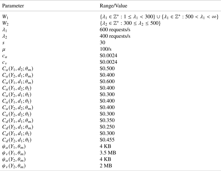
In this section, we numerically verify the theorems proved in the previous section and obtain some insights into how the traffic dropping probabilities affect the expected payoffs of both the attacker and the defender. For the purpose of numerical verification, we consider the parameter values as given in Table 3.

Table 3.

Parameters and their values

Using the values given in Table 3, the EAFs are $\textit{EAF}_1^{\theta _m} = {\psi _v(Y_1; \theta _m)}/{\psi _a(Y_1; \theta _m)} = 896$ and $\textit{EAF}_2^{\theta _m} = {\psi _v(Y_2; \theta _m)}/{\psi _a(Y_2; \theta _m)} = 512$ so that the amplifications are in the range of traditional amplifications [Reference Rossow21], that is, between 318 and 1395. For legitimate traffic, no amplification is produced, hence we assume that $\textit{EAF}_{i}^{\theta _l} = 1$ for each $i \in \{1,2\}$. It should be noted that these parameter values are taken only for the purpose of numerical illustration.

6.1. Numerical example of pooling PBE

Suppose Nature's probability distribution $p = 0.5$. Furthermore, let us take $P_d(Y_1,d_1) = 0.7$, $P_d(Y_2,d_1)=0.45$ such that we have:

\begin{align*} & P_d(Y_1, d_2) = 0,\\ & 1 - \frac{(\frac{\lambda_2}{s\mu} + \textit{EAF}_2^{\theta_m})\{1 - P_d(Y_2,d_1)\} + C_a(Y_1, d_2; \theta_m) - C_a(Y_2, d_1; \theta_m)}{(\frac{\lambda_1}{s\mu} + \textit{EAF}_1^{\theta_m})} = 0.6856,\\ & 1 - \frac{(\frac{\lambda_2}{s\mu} + \textit{EAF}_2^{\theta_l})\{1 - P_d(Y_2,d_1)\} + C_a(Y_1, d_2;\theta_l) - C_a(Y_2, d_1;\theta_l)}{(\frac{\lambda_1}{s\mu} + \textit{EAF}_1^{\theta_l})} = 0.3972,\\ & 1 - \frac{(\frac{\lambda_1}{s\mu} + \textit{EAF}_1^{\theta_m})\{1 - P_d(Y_2,d_1)\} + C_a(Y_2, d_1;\theta_m) - C_a(Y_1, d_1; \theta_m)}{(\frac{\lambda_2}{s\mu} + \textit{EAF}_2^{\theta_m})} = 0.4754,\\ & 1 - \frac{(\frac{\lambda_1}{s\mu} + \textit{EAF}_1^{\theta_l})\{1 - P_d(Y_2,d_1)\} + C_a(Y_2, d_1; \theta_l) - C_a(Y_1, d_1; \theta_l)}{(\frac{\lambda_2}{s\mu} + \textit{EAF}_2^{\theta_l})} = 0.7706, \end{align*}

and

\begin{align*} & \frac{C_d(Y_1, d_1; \theta_m)}{(\frac{\lambda_1}{s\mu} + \textit{EAF}_1^{\theta_m})} = 0.00039,\\ & \frac{C_d(Y_1, d_1; \theta_l)}{(\frac{\lambda_1}{s\mu} + \textit{EAF}_1^{\theta_l})} =0.2500,\\ & \frac{C_d(Y_2, d_1;\theta_m)}{(\frac{\lambda_2}{s\mu} + \textit{EAF}_2^{\theta_m})} = 0.00048,\\ & \frac{C_d(Y_2, d_1; \theta_l)}{(\frac{\lambda_2}{s\mu} + \textit{EAF}_2^{\theta_l})} = 0.4015, \end{align*}

and the condition of Theorem 1 is satisfied.

Attacker's expected payoff matrix 1

\begin{align*}\begin{matrix}& \begin{matrix}d_1^{Y_1}d_1^{Y_2} & & d_1^{Y_1}d_2^{Y_2} & & d_2^{Y_1}d_1^{Y_2} & & d_2^{Y_1}d_2^{Y_2}\ \end{matrix} \\ \begin{matrix}Y_1|_{\theta_m}Y_2|_{\theta_l} \\ Y_2|_{\theta_m}Y_2|_{\theta_l}\end{matrix} & \begin{bmatrix}134.2417 & 134.5467 & 447.9617 & 448.2667\\ 140.7483 & 256.2833 & 140.7483 & 256.2833 \end{bmatrix}\end{matrix}\end{align*}

Defender's expected payoff matrix 1

\begin{align*}\begin{matrix}& \begin{matrix}d_1^{Y_1}d_1^{Y_2} & & & d_1^{Y_1}d_2^{Y_2} & & & d_2^{Y_1}d_1^{Y_2} & & d_2^{Y_1}d_2^{Y_2}\end{matrix} \\ \begin{matrix}Y_1|_{\theta_m}Y_2|_{\theta_l} \\ Y_2|_{\theta_m}Y_2|_{\theta_l}\end{matrix} & \begin{bmatrix}-135.1442 & -135.1717 & -448.6392 & -448.6667\\ -141.5008 & -256.6333 & -141.5008 & - 256.6333\end{bmatrix}\end{matrix}\end{align*}

It is easy to check from the above expected payoff matrices that

$(Y_2|\theta _mY_2|\theta _l,\ d_1^{Y_1}d_1^{Y_2})$ is the pooling PBE as derived in Theorem 1. In the pooling equilibrium, both the malicious ($\theta _m$) and regular type ($\theta _l$) attacker perform the same action $Y_2$ and the defender responds to the attacker by choosing the action $d_1$. Hence, the attacker's type is not completely revealed to the defender.

6.2. Numerical example of separating PBE

Now, let us suppose that $P_d(Y_1,d_1) = 0.6$, $P_d(Y_2,d_1)=0.4$. Then,

\begin{align*} & 1 - \frac{(\frac{\lambda_1}{s\mu} + \textit{EAF}_1^{\theta_m})\{1 - P_d(Y_2,d_1)\} + (K_a^{2} - K_a^{1})}{(\frac{\lambda_2}{s\mu} + \textit{EAF}_2^{\theta_m})} = 0.3004,\\ & \frac{C_d(Y_1, d_1; \theta_m)}{(\frac{\lambda_1}{s\mu} + \textit{EAF}_1^{\theta_m})} = 0.00039,\\ & \frac{C_d(Y_1, d_1; \theta_l)}{(\frac{\lambda_1}{s\mu} + 1)} = 0.2500,\\ & \frac{C_d(Y_2, d_1; \theta_m)}{(\frac{\lambda_2}{s\mu} + \textit{EAF}_2^{\theta_m})} = 0.00048,\\ & \frac{C_d(Y_2, d_1; \theta_l)}{(\frac{\lambda_2}{s\mu} + 1)} = 0.4015, \end{align*}

and the condition of Theorem 2 is satisfied.

Attacker's expected payoff matrix 2

\begin{align*}\begin{matrix}& \begin{matrix}d_1^{Y_1}d_1^{Y_2} & & d_1^{Y_1}d_2^{Y_2} & & d_2^{Y_1}d_1^{Y_2} & & d_2^{Y_1}d_2^{Y_2}\end{matrix}\\ \begin{matrix}Y_1|_{\theta_m}Y_2|_{\theta_l}\\ Y_2|_{\theta_m}Y_2|_{\theta_l}\end{matrix} & \begin{bmatrix}179.0517 & 179.3567 & 447.9617 & 448.2667\\140.7483 & 256.2833 & 140.7483 & 256.2833\end{bmatrix}\end{matrix}\end{align*}

Defender's expected payoff matrix 2

\begin{align*}\begin{matrix}& \begin{matrix} d_1^{Y_1}d_1^{Y_2} & & \ \ \ d_1^{Y_1}d_2^{Y_2} & & \ \ d_2^{Y_1}d_1^{Y_2} & & \ \ d_2^{Y_1}d_2^{Y_2} \end{matrix}\\\begin{matrix}Y_1|_{\theta_m}Y_2|_{\theta_l}\\ Y_2|_{\theta_m}Y_2|_{\theta_l}\end{matrix} & \begin{bmatrix}-179.9542 & -179.9817 & -448.6392 & -448.6667\\-141.5008 & -256.6333 & -141.5008 & -256.6333\end{bmatrix}\end{matrix}\end{align*}

It can be noticed easily from the above expected payoff matrices that

$(Y_1|\theta _mY_2|\theta _l,\ d_1^{Y_1}d_1^{Y_2})$ is the separating PBE as obtained in Theorem 2. In the separating equilibrium, different types of the attacker performs different actions, that is, the attacker performs the action $Y_1$ if he/she is malicious ($\theta _m$), whereas he/she performs the action $Y_2$ if he/she is legitimate ($\theta _l$). In this case, the attacker's type is completely revealed to the defender and the defender responds to the attacker by choosing the action $d_1$.

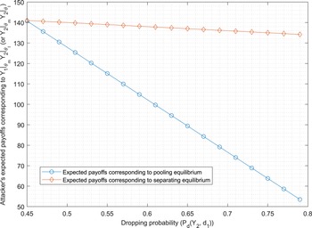
We now compute the pooling and separating PBE for different values of the traffic dropping probability $P_d(Y_2,d_1)$ and plot the expected payoffs corresponding to these equilibria as shown in Figures 4 and 5. In Figure 4, it can be observed that when the dropping probability of the action $Y_2$ increases, the attacker's expected payoff decreases in the case of both pooling and separating equilibrium. Moreover, for the pooling equilibrium, the expected payoff decreases significantly as compared with the separating equilibrium. This can be seen from the fact that in the pooling equilibrium, the attacker uses the strategy $Y_2|_{\theta _m} Y_2|_{\theta _l}$. That is, both types of the attacker (malicious ($\theta _m$) and legitimate ($\theta _l$)) perform the same action $Y_2$ and the defender responds to it by taking the action $d_1$ with dropping probability $P_d(Y_2, d_1)$. On the other hand, in the case of separating equilibrium, the attacker uses the strategy $Y_1|_{\theta _m}Y_2|_{\theta _l}$. That is, only the legitimate type attacker performs the action $Y_2$ and the defender responds to it by choosing the action $d_1$ with dropping probability $P_d(Y_2, d_1)$. Hence, the expected payoff of the attacker in the case of separating equilibrium decreases relatively slower when compared with the expected payoffs corresponding to the pooling equilibrium.

Figure 4.

Dropping probability versus attacker's expected payoffs.

Figure 5.

Dropping probability versus defender's expected payoffs.

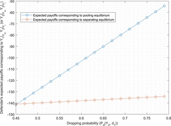
Furthermore, from Figure 5, it can be noticed that the defender's expected payoff corresponding to the pooling equilibrium increases much faster than that of the separating equilibrium. As in the case of the attacker's expected payoffs, the defender's expected payoffs are also affected with respect to the dropping probability $P_d(Y_2, d_1)$. This is due to the fact that in the pooling equilibrium, the action $Y_2$ performed by both types of the attacker (malicious ($\theta _m$) and legitimate ($\theta _l$)) is responded by the defender with the action $d_1$ and dropping probability $P_d(Y_2, d_1)$. However, in the case of separating equilibrium, only the legitimate type attacker performs the action $Y_2$ and this action is dealt with by the defender with the action $d_1$ and dropping probability $P_d(Y_2, d_1)$. Thus, we have observed the expected results from the above discussion that the greater the traffic dropping probability of the attacker's action, the smaller the expected payoffs maximized by the attacker (i.e., Figure 4) and the higher the expected payoffs of the defender (i.e., Figure 5).

6.3. Numerical example of mixed strategy PBE

Let us take $P_d(Y_1,d_1) = 0.6$, $P_d(Y_2,d_1)=0.4$. We have:

\begin{align*} & 1 - \frac{(\frac{\lambda_2}{s\mu} + \textit{EAF}_2^{\theta_m})\{1 - P_d(Y_2,d_2)\} + \{C_a(Y_1, d_1;\theta_m) - C_a(Y_2, d_2;\theta_m)\}}{(\frac{\lambda_1}{s\mu} + \textit{EAF}_1^{\theta_m})} = 0.4283,\\ & 1 - \frac{(\frac{\lambda_1}{s\mu} + \textit{EAF}_1^{\theta_m})\{1 - P_d(Y_1,d_1)\} + \{C_a(Y_2, d_1;\theta_m) - C_a(Y_1, d_1;\theta_m)\}}{(\frac{\lambda_2}{s\mu} + \textit{EAF}_2^{\theta_m})} = 0.3004,\\ & \frac{C_d(Y_2, d_1;\theta_l)}{(\frac{\lambda_2}{s\mu}+\textit{EAF}_2^{\theta_l})}= 0.4015, \\ & \frac{pC_d(Y_2, d_1;\theta_m) + (1 - p) C_d(Y_2, d_1;\theta_l)}{p\textit{EAF}_2^{\theta_m} + (1 - p) \textit{EAF}_2^{\theta_l}+ \frac{\lambda_2}{s\mu}} = 0.0014,\\ & \frac{C_d(Y_1, d_1;\theta_m)}{(\frac{\lambda_1}{s\mu}+\textit{EAF}_1^{\theta_m})} = 0.00039. \end{align*}

Therefore, the condition of Theorem 3 is satisfied and thus we have a mixed strategy PBE which is described by the following mixed strategy probabilities:

$$\omega^{*} = \frac{\alpha_{22} - \alpha_{12}}{(\alpha_{22} - \alpha_{12}) + (\alpha_{11} - \alpha_{21})}= 0.751\quad \text{and}\quad \xi^{*}_{\theta_m} = \frac{\beta_{12} - \beta_{11}}{(\beta_{12} - \beta_{11}) + (\beta_{21} - \beta_{22})} = 0.0000081.$$

Thus, at the mixed strategy PBE, the attacker chooses his/her strategies $Y_2|_{\theta _m}Y_2|_{\theta _l}$ and $Y_1|_{\theta _m}Y_2|_{\theta _l}$ with probabilities $\xi ^{*}_{\theta _m} = 0.0000081$ and $1 - \xi ^{*}_{\theta _m} = 0.9999919$, respectively. And since $\delta = 1$, the defender chooses its strategies $d_1^{Y_1}d_1^{Y_2}$, $d_1^{Y_1}d_2^{Y_2}$, $d_2^{Y_1}d_1^{Y_2}$ and $d_2^{Y_1}d_2^{Y_2}$ with probabilities $\delta \omega ^{*} = 0.751$ and $\delta (1 - \omega ^{*}) = 0. 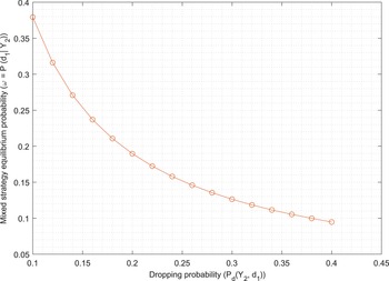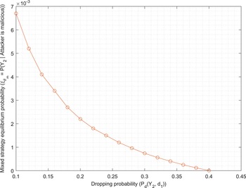249$, $(1-\delta )\omega ^{*} = 0$, $(1 - \delta )(1-\omega ^{*}) = 0$, respectively. To illustrate how the mixed strategy equilibria are affected by the dropping probability, we determine the mixed strategy PBE for different values of the dropping probability $P_d(Y_2, d_1)$ and plot them as shown in Figures 6 and 7. We know that $\omega = P(d_1|Y_2)$ is the probability that the defender chooses the action $d_1$ given that the action $Y_2$ is performed by the attacker. Therefore, it can be seen from Figure 6 that when the dropping probability of traffic resulting from the action $Y_2$ increases, the probability with which the defender chooses the action $d_1$ decreases at the equilibrium points. In addition, we know that $\xi _{\theta _m} = P(Y_2|Attacker\ is\ malicious)$ is the probability that the attacker chooses action $Y_2$ given that his/her type is malicious ($\theta _m$). Hence, as the dropping probability $P_d(Y_2, d_1)$ of action $Y_2$ increases, the probability with which the attacker chooses action $Y_2$ decreases at the equilibrium points as shown in Figure 7.

Figure 6.

Dropping probability versus mixed strategy equilibrium probability ($\omega$).

Figure 7.

Dropping probability versus mixed strategy equilibrium probability ($\xi _{\theta _m}$).