1 Introduction
Falling objects, such as leaves in the air or coins dropped into water, have long been captivating scientists from Newton to Maxwell. Recent research revealed that these smooth, yet articulate, motions contain rich and complex fluid–structure interaction (FSI). A simple representation is how a plate falls within a fluid medium, and disrupts the still flow. The disruption generates differences in the pressure distributions above, below and along the planform surfaces, providing a lift,
 $L$
, to passively sustain a plate in flight. Paper cards, plants seeds, sedimentation of marine micro-organisms and particles represent a profound range of heavy falling objects in natural flight. It is thus compelling to investigate how they develop flight characteristics as they fall. With reference to previous studies, the transition from falling to flight is associated with a range of plate densities and fluid viscosities, and their coupling throughout the unsteady process. As there is a mapping of flight states for light plates, it is desirable to extend and fulfil the mapping for heavy plates (dimensionless moment of inertia
 $I^{\ast }>1$
) to understand natural flight in the biological and atmospheric realms, as well as for application to sustaining vehicular flight by harvesting potential energy.
Studies have experimentally revealed that, with respect to
 $I^{\ast }$
, and the Reynolds number
 $Re$
, plates would tumble in one direction, flutter side to side or steadily fall (Dupleich Reference Dupleich1941; Willmarth, Hawk & Harvey Reference Willmarth, Hawk and Harvey1964; Belmonte et al.
Reference Belmonte, Shelley, Eldakar and Wiggins2001; Andersen, Pesavento & Wang Reference Andersen, Pesavento and Wang2005a
; Zhong et al.
Reference Zhong, Lee, Su, Chen, Zhou and Wu2013). These are the elementary flight states that make up the trajectories within the two-dimensional domain. Recently, direct numerical simulation (DNS) has greatly enriched the mapping of flight states for a range of
 $I^{\ast }$
and
 $Re$
(Fonseca & Herrmann Reference Fonseca and Herrmann2005; Auguste, Magnaudet & Fabre Reference Auguste, Magnaudet and Fabre2013; Chrust, Bouchet & Dušek Reference Chrust, Bouchet and Dušek2013; Wu & Lin Reference Wu and Lin2015). DNS has also provided an in-depth understanding of FSI, especially at the low to intermediate Reynolds number regime of
 $Re\sim O(10^{2})$
in which viscous effects are important. The relationship between
 $I^{\ast }$
and wake patterns for the case with two-dimensional cylinders (Mathai et al.
Reference Mathai, Zhu, Sun and Lohse2017) and three-dimensional discs (Dušek, Chrust & Bouchet Reference Dušek, Chrust and Bouchet2016) have explored wake patterns with respect to the weight of the solid and the viscosity of the fluid.
Apart from the elementary flight states of stable falling, fluttering and tumbling, the transition phases among the states have also been important concerns. Field, Klaus & Moore (Reference Field, Klaus and Moore1997) studied the instabilities of chaotic trajectories within the envelope of the flight map between fluttering and tumbling. At low
 $I^{\ast }$
, the transition from stable falling to fluttering through the increase of
 $Re$
may undergo low frequency meandering or high frequency erratic oscillation (Ern et al.
Reference Ern, Risso, Fabre and Magnaudet2012). This was also depicted as the quasi-vertical or transitional state (Chrust et al.
Reference Chrust, Bouchet and Dušek2013; Wu & Lin Reference Wu and Lin2015). The transition between falling and fluttering is dynamically subcritical, located about a heteroclinic orbit (Auguste et al.
Reference Auguste, Magnaudet and Fabre2013; Hu & Wang Reference Hu and Wang2014). A small change in the system parameters, predominately
 $Re$
in this case, may topple the plate steadily fall towards a fixed point, or away to a fluttering limit cycle.
In establishing a general theoretical model of falling flight, the flow resistance of the body was first asserted over a century ago by Maxwell (Reference Maxwell and Harman1852), whose work affirmed periodic rotation when the falling body is subjected to air resistance. Further development led to Kirchhoff’s time-dependent ordinary differential equation; and the FSI was realised as a Hamiltonian dynamical system (Lamb Reference Lamb1945), further portraying periodic as well as chaotic behaviours through limit cycles (Kuznetsov Reference Kuznetsov2015). The consideration of rotational lift in the model of Pesavento & Wang (Reference Pesavento and Wang2004) provided the local effect of climb during fluttering and tumbling flights (Andersen et al. Reference Andersen, Pesavento and Wang2005a ; Wang et al. Reference Wang, Hu, Xu and Wu2013). In depicting the divergence of a limit cycle or a flight state, the galloping notion of stability was studied but with drawbacks. The quasi-steady model has been proven to be limited in determining angular movement; the nonlinear model is found to be acceptable at low amplitude motion; the unsteady model, while it is the most accurate, requires specific experimental efforts in determining the aerodynamic coefficients (Paidoussis, Price & Langre Reference Paidoussis, Price and Langre2011).
Contrary to DNS and experimental results that showed the invariance of flight paths to initial conditions (Andersen, Pesavento & Wang Reference Andersen, Pesavento and Wang2005b
; Wan, Dong & Liang Reference Wan, Dong and Liang2012), resulting in unique limit cycles, numerical solutions of the dynamic model suggested multiple limit cycles are possible in relation to steady fall (Kuznetsov Reference Kuznetsov2015). Experimental findings with falling disks suggested that tumbling motions were found at
 $I^{\ast }\sim O(10^{0})$
and stable falling at
 $I^{\ast }\sim O(10^{2})$
(Heisinger, Newton & Kanso Reference Heisinger, Newton and Kanso2014); whereas results with autorotating wings reported tumbling motion at
 $I^{\ast }\sim O(10^{1})$
(Smith Reference Smith1971). Further development of the theoretical model suggested that the earlier findings of heavy plate fluttering were part of the prolonged development towards tumbling flight (Hu & Wang Reference Hu and Wang2014). More interestingly, the possibility of different flight states was also reported for heavy disks (Chrust et al.
Reference Chrust, Bouchet and Dušek2013; Dušek et al.
Reference Dušek, Chrust and Bouchet2016) under the same
 $I^{\ast }$
and
 $Re$
. The perplexity of these different findings raises new interests about the nature of passive flight for heavy plates.
The effects of shape and thickness-to-length ratios also led to interesting findings. Wu & Lin (Reference Wu and Lin2015) recorded a faster lateral and descent velocity, but slower rotational speed, for rectangular plates in comparison to elliptical ones. Mittal, Seshadri & Udaykumar (Reference Mittal, Seshadri and Udaykumar2004) determined wake instabilities of autorotation in relation to thickness and Reynolds number. Furthermore, the increase in thicknesses also increases the oscillation angles and the tendency of transition from fluttering to tumbling (Wang et al. Reference Wang, Shu, Teo and Yang2016).
Thus far, experimental and numerical studies of heavy plates at large
 $I^{\ast }$
remain sparse. While there have been observations of heavy plates under elementary flight motion, the transition from stable falling to sustainable flight remains to be thoroughly captured and explained. Therefore, the present study continues from previous works, and investigates the passive engagement of tumbling flight from heavy falling. To portray the dynamics of unsteady interactions between the fluid and the solid, the immersed boundary (IB) method (Huang, Shin & Sung Reference Huang, Shin and Sung2007) is used for its adaptability to a moving body interacting with a viscous fluid. The free fall specimen used is a thin rectangular plate for the examination of changes in weight. Results are presented in the sequence from heavy falling to tumbling flight. The trajectory developments are analysed through phase portraits and time histories. Investigation of the initial angle of release from rest,
 $\unicode[STIX]{x1D703}_{0}$
, leads to the finding of bistabilty, where stable falling and tumbling are both possible. The mechanism that gives rise to the two states is discussed through the recirculating flow and the relation of
 $\unicode[STIX]{x1D703}_{0}$
to the lift curve, followed by an investigation on the effect of plate shape.
2 Numerical method
The plate is considered as an immersed body with thickness
 $h$
, and chord length
 $l$
. The density of the solid
 $\unicode[STIX]{x1D70C}_{s}$
is higher than that of the fluid
 $\unicode[STIX]{x1D70C}_{f}$
, such that it falls under the field of gravity
 $\boldsymbol{g}$
(and
 $g=|\boldsymbol{g}|$
) inside the fluid of viscosity
 $\unicode[STIX]{x1D707}$
. When the fall is initiated, the solid generates a flow velocity field
 $\boldsymbol{u}=(u_{x},u_{y})$
in the Eulerian reference frame. The convention of using
 $\unicode[STIX]{x1D70C}_{f}$
,
 $l$
and the average descent velocity
 $V_{\infty }=[2(\unicode[STIX]{x1D70C}_{s}/\unicode[STIX]{x1D70C}_{f}-1)gh]^{1/2}$
as the characteristic scales is followed (Andersen et al.
Reference Andersen, Pesavento and Wang2005b
; Auguste et al.
Reference Auguste, Magnaudet and Fabre2013). The subsequent dimensionless parameters are: thickness ratio
 $h^{\ast }=h/l$
, density ratio
 $\unicode[STIX]{x1D70C}^{\ast }=\unicode[STIX]{x1D70C}_{s}/\unicode[STIX]{x1D70C}_{f}$
and Reynolds number
 $Re=\unicode[STIX]{x1D70C}_{f}lV_{\infty }/\unicode[STIX]{x1D707}$
. The Navier–Stokes (NS) equations (2.1) and the continuity equation (2.2) for incompressible flow are presented below in non-dimensional form. The linear and angular equations of motion of the rigid plate, also non-dimensionalised, are denoted by (2.3) and (2.4), respectively.
 $$\begin{eqnarray}\displaystyle & \displaystyle \frac{\text{D}\boldsymbol{u}}{\text{D}t}=-\unicode[STIX]{x1D735}p+Re^{-1}\unicode[STIX]{x1D6FB}^{2}\boldsymbol{u}+\boldsymbol{f}, & \displaystyle\end{eqnarray}$$
 $$\begin{eqnarray}\displaystyle & \displaystyle \unicode[STIX]{x1D735}\boldsymbol{\cdot }\boldsymbol{u}=0, & \displaystyle\end{eqnarray}$$
 $$\begin{eqnarray}\displaystyle & \displaystyle \frac{\text{d}\boldsymbol{V}}{\text{d}t}=\frac{-\boldsymbol{F}}{\unicode[STIX]{x1D70C}^{\ast }}-\left[\frac{3\unicode[STIX]{x03C0}I^{\ast }}{4(1+h^{\ast })}-2h^{\ast }\right]^{-1}\frac{\boldsymbol{g}}{g}, & \displaystyle\end{eqnarray}$$
 $$\begin{eqnarray}\displaystyle & \displaystyle \frac{\text{d}V_{\unicode[STIX]{x1D703}}}{\text{d}t}=\frac{32\unicode[STIX]{x1D70F}}{\unicode[STIX]{x03C0}I^{\ast }}. & \displaystyle\end{eqnarray}$$
Here,
 $\boldsymbol{F}=(F_{x},F_{y})$
and
 $\boldsymbol{f}=(f_{x},f_{y})$
are the interaction forces between the fluid and the solid. Analogously,
 $\unicode[STIX]{x1D70F}$
denotes the torque from the fluid forces applied to the solid, calculated from the summation of
 $\boldsymbol{f}$
acting on the centre of mass of the solid. The force of fluid in (2.3) is shown to account for the density difference through
 $\unicode[STIX]{x1D70C}^{\ast }$
. Introducing the moment of inertia through
 $I^{\ast }=8\unicode[STIX]{x1D70C}^{\ast }h^{\ast }(1+h^{\ast })/3\unicode[STIX]{x03C0}$
for rectangular plates (Andersen et al.
Reference Andersen, Pesavento and Wang2005b
), and with the current case of
 $h^{\ast }\ll 1$
, equation (2.3) takes the form
 $\text{d}\boldsymbol{V}/\text{d}t=(4\unicode[STIX]{x03C0}/3I^{\ast })(-2h^{\ast }\boldsymbol{F}-\boldsymbol{g}/g)$
illustrating the relative fluid and gravitational force contributions.
In the IB method, the interaction between the Lagrangian points and the adjacent fluid particle is given by a force feedback law (Huang et al. Reference Huang, Shin and Sung2007):
 $$\begin{eqnarray}\displaystyle \boldsymbol{F}=k_{a}\int _{0}^{t}(\boldsymbol{U}_{IB}-\boldsymbol{V})\,\text{d}t+k_{b}(\boldsymbol{U}_{IB}-\boldsymbol{V}), & & \displaystyle\end{eqnarray}$$
where
 $k_{a}$
and
 $k_{b}$
are large negative constants,
 $\boldsymbol{U}_{IB}$
is the fluid velocity interpolated at the Lagrangian points and
 $\boldsymbol{V}$
is the Lagrangian velocity of the plate. Interpolation from the Eulerian fluid velocity to the Lagrangian points is done via a four-point regularised delta function (Peskin Reference Peskin2002):
 $$\begin{eqnarray}\displaystyle \boldsymbol{U}_{IB}(s,t)=\int _{domain}\boldsymbol{u}(\boldsymbol{x},t)\unicode[STIX]{x1D6FF}(\boldsymbol{X}(s,t)-\boldsymbol{x})\,\text{d}\boldsymbol{x}. & & \displaystyle\end{eqnarray}$$
Conversely, the force from the solid acting on the fluid is calculated by the spreading of the Lagrangian force to its nearby Eulerian grid through:
 $$\begin{eqnarray}\displaystyle \boldsymbol{f}(x,t)=\int _{IB}\boldsymbol{F}(s,t)\unicode[STIX]{x1D6FF}(\boldsymbol{x}-\boldsymbol{x}(s,t))\,\text{d}s. & & \displaystyle\end{eqnarray}$$
For clarity, the IB equations (2.6) and (2.7) have lower case symbols representing Eulerian quantities, and upper case denotes Lagrangian variables. The arclength of the solid surface is denoted by
 $s$
. The fluid motion equations are then discretised with the finite difference method on a staggered grid. The velocity components and momentum forcing are defined on the cell interfaces, whereas the pressure is applied at the centres of cells. Decoupling of the velocity and pressure is achieved by the upper/lower block decomposition through approximate factorisation. The fractional step method is used for temporal advancement, and both the convective and viscous terms are discretised via the Crank–Nicholson scheme that preserves the second-order temporal accuracy (Kim, Kim & Choi Reference Kim, Kim and Choi2001). The pressure Poisson equation is solved by a direct method using fast Fourier transform, which is then used to correct the velocity field to satisfy the continuity equation in completing the fractional steps. Moving from the fluid to the solid, velocities from (2.6) are used to solve (2.3) and (2.4) via the fourth-order Runge–Kutta method. Finally, the resulting momentum forcing is exerted on the flow through (2.7).
For each simulating run, the plate begins to fall from rest and begins its motion at a distance of
 $2l$
from the upper boundary of the Eulerian domain of size 32 or 64 by
 $16l$
by which the dynamics has been validated to be unaffected at this proximity. The thickness ratio of the plate is kept small, i.e.
 $h^{\ast }=1/128$
. This is the nominal value used, unless otherwise stated, to isolate the changes of aerodynamic effects due to geometrical differences. Trajectories are sufficiently developed over time for subsequent analyses.
Comparison of DNS results for mean periodic velocities for the steady flight states of elliptical plates with
 $h^{\ast }=1/8$
.
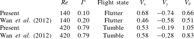
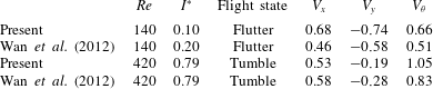
Table 1 is a comparison of numerical results of steady state velocities in the vertical, lateral and angular components for ellipses between the present simulations and the literature (Wan et al.
Reference Wan, Dong and Liang2012) in two elementary flight states. Results are in good agreement within the range of
 $Re$
and
 $I^{\ast }$
for both fluttering and tumbling. In the case of fluttering,
 $I^{\ast }$
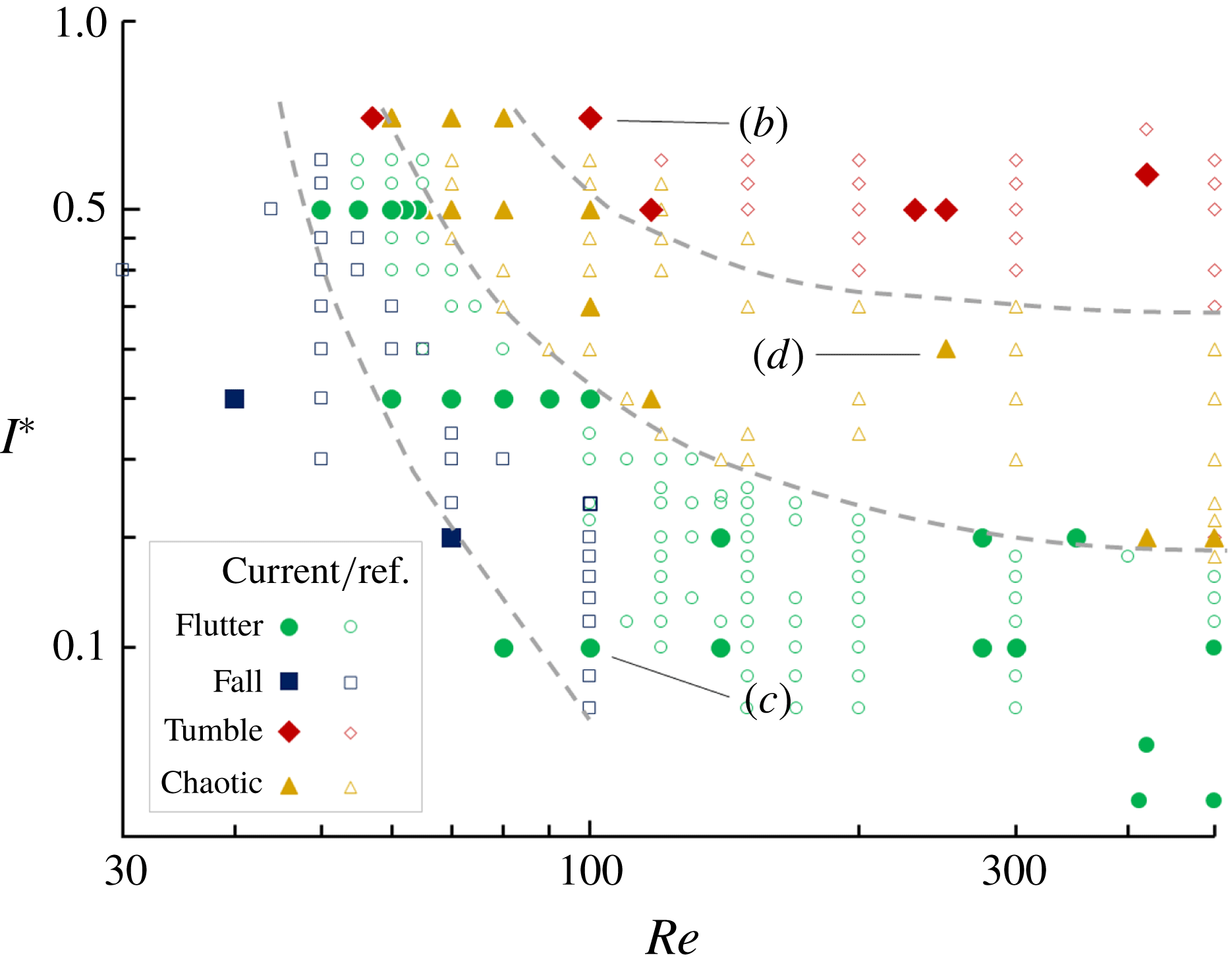
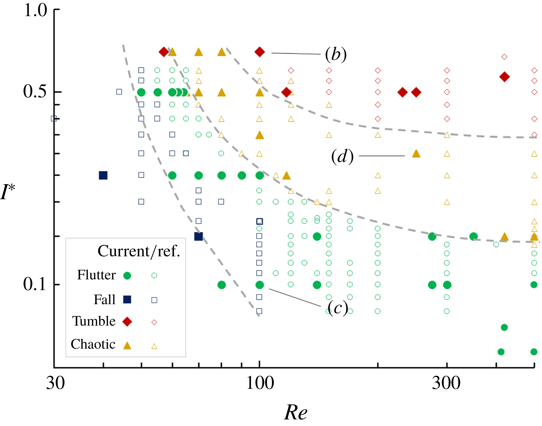
is reduced to ensure the stability of stable flight, i.e. away from the fluttering–chaotic boarder in figure 3. In compensating for this difference, an adjustment factor is multiplied by the base of the velocities in the relationship
 $V\propto (\unicode[STIX]{x1D70C}^{\ast })^{1/2}$
. This ‘penalty’ has the greatest effect on
 $V_{x}$
as the lateral motion should be less affected by the relative density (cf.
 $V_{x}$
for tumbling). While deviations are expected in simulating unsteady flows (Wu & Lin Reference Wu and Lin2015), results in table 1 for both fluttering and tumbling match satisfactorily overall.
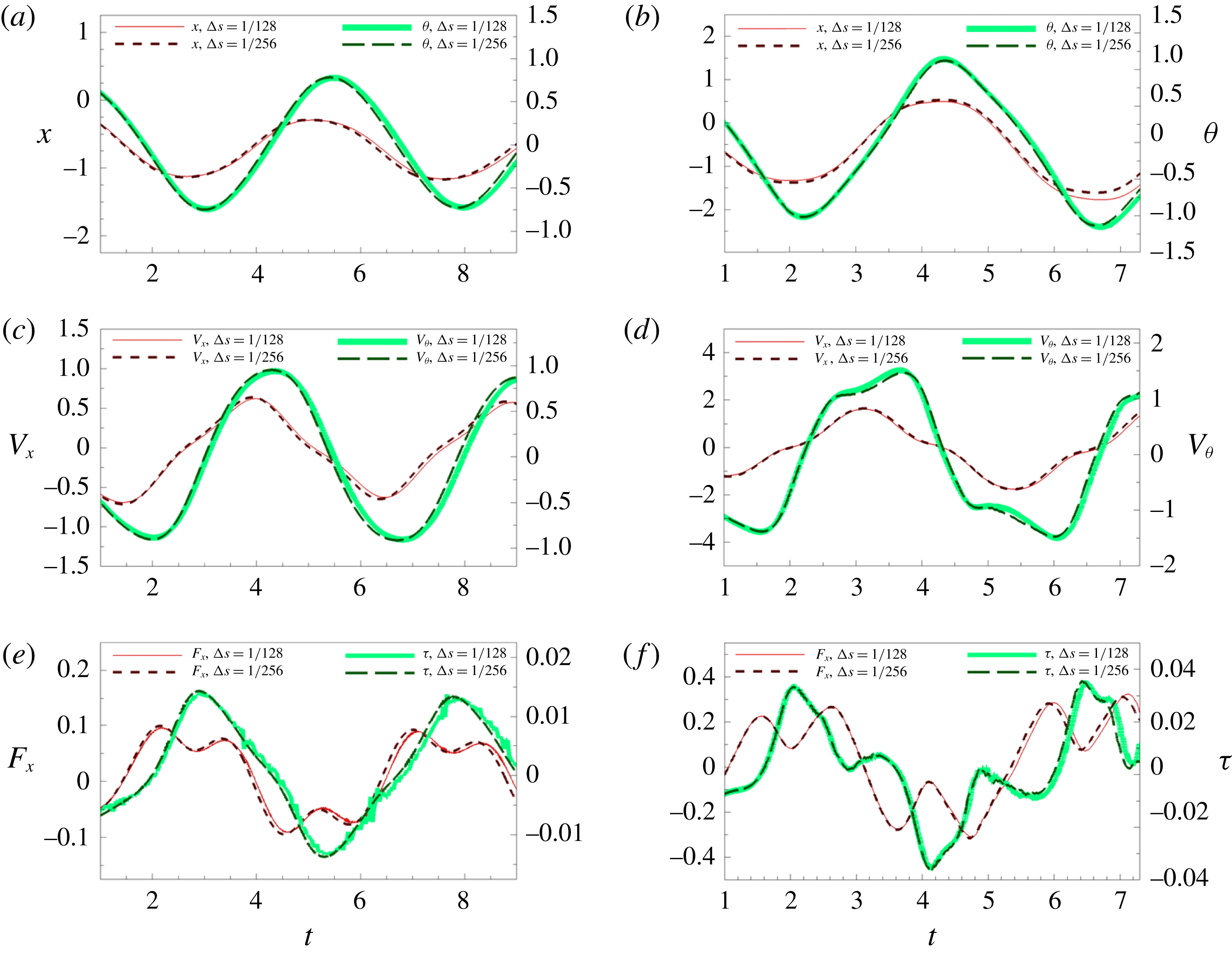
The performance of the numerical method is evaluated at different grid spacings through the lateral and angular dynamics. A light fluttering plate is chosen for its periodicity and stability of its flight path. The Eulerian and Lagrangian grid spacings are set to be the same, represented by
 $\unicode[STIX]{x0394}s$
, normalised with respect to
 $l$
; and the Courant number
 $u\unicode[STIX]{x0394}t/\unicode[STIX]{x0394}s<0.5$
is maintained. Two thicknesses of rectangles are tested in figure 1, i.e.
 $h^{\ast }=1/128$
in (a,c,e) and
 $h^{\ast }=1/18$
in (b,d,f). The dynamics in the
 $\unicode[STIX]{x0394}s=1/128$
lags slightly behind in displacements, velocities, force and torque, as shown in figures 1(a,b), 1(c,d) and 1(e,f), respectively. Note that, at
 $h^{\ast }=1/18$
, the rectangular plate exhibits more complex dynamics. Slight fluctuations of torque
 $\unicode[STIX]{x1D70F}$
are seen in (e) and (f) for
 $\unicode[STIX]{x0394}s=1/128$
, which are suspected to be a result of the moment arm amplifying the application of the fluid forces onto the plates. Fluctuation is reduced for
 $\unicode[STIX]{x0394}s=1/256$
as the forces are more precisely applied on the IB. In general, both grid spacings converge to identical history profiles for different plates while the flight mechanics and flight states are generally not affected. In the subsequent simulations, a grid spacing of
 $\unicode[STIX]{x0394}s=1/128$
is chosen for computational efficiency unless otherwise stated. The coefficients in (2.5) need to be sufficiently high to maintain artificial stiffness among the Lagrangian points, such that they interact within sufficient proximity to the corresponding fluid particles, but avoiding numerical stability issues with the time steps. The simulations here adopt the constants as
 $k_{a}=-10^{5}$
and
 $k_{b}=-10^{2}$
(Huang et al.
Reference Huang, Shin and Sung2007).
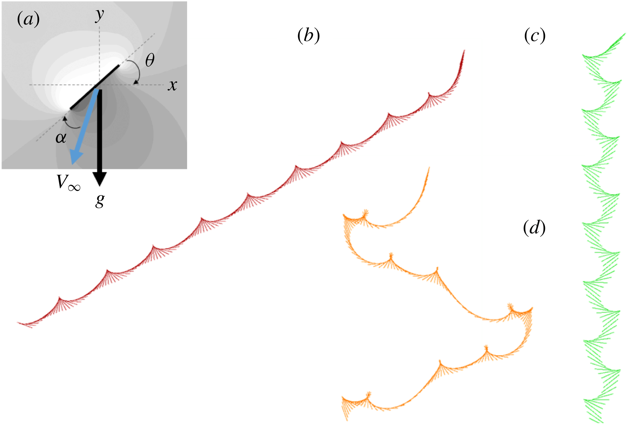
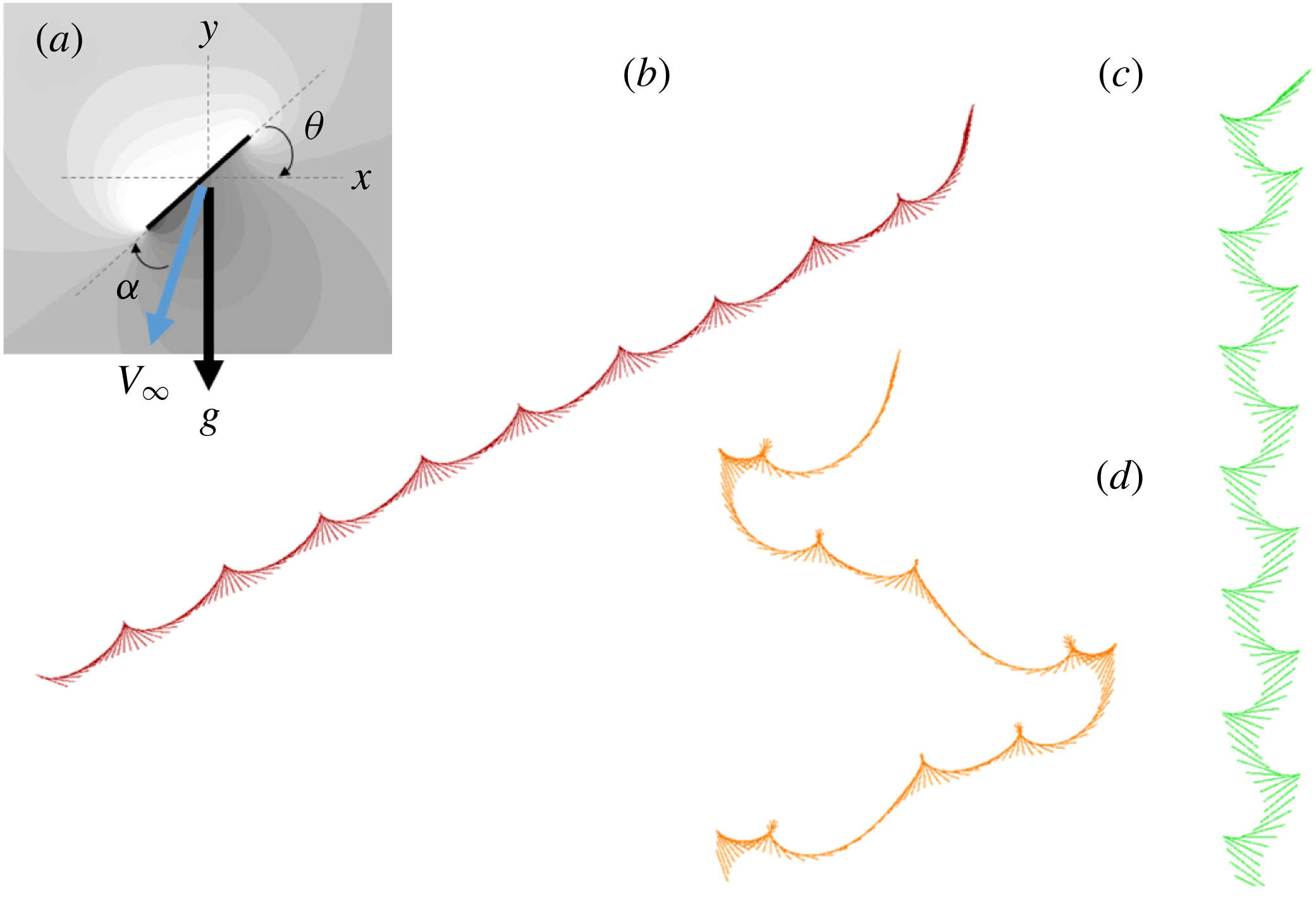
Figure 2(a) is the Cartesian reference frame and the associated symbols. Simulations of the basic flight states, i.e. tumbling, flutter and chaotic, are presented in figure 2(b–d). The map of figure 3 also shows that the current flight states are well depicted for light plates of
 $I^{\ast }<1$
and in good agreement with previous studies. Note there appears a slight margin at the boarder between stable falling and fluttering, subject to how lateral oscillations are perceived for different studies. Here, this boarder is based on the definition of stable falling presented in § 3.1.
Time histories of fluttering at
 $Re=80$
,
 $I^{\ast }=0.1$
and
 $\unicode[STIX]{x1D703}_{0}=45^{\circ }$
for different Lagrangian grid sizes
 $\unicode[STIX]{x0394}s$
of rectangular plates. (a,b) Displacements, (c,d) velocities and (e,f) forces for plates of thicknesses (a,c,e)
 $h^{\ast }=1/128$
, and (b,d,f)
 $h^{\ast }=1/18$
.

(a) Reference frame of the global Cartesian coordinate; (b–d) simulation results for tumbling, fluttering and chaotic flight states.
A map of flight states for light plates of
 $I^{\ast }<1$
. Current and reference DNS results are plotted together, showing the relative regions of stable flight states separated by dashed lines (Kolomenskiy & Schneider Reference Kolomenskiy and Schneider2009; Wan et al.
Reference Wan, Dong and Liang2012; Wu & Lin Reference Wu and Lin2015). Labels (b–d) correspond to the cases in figure 2.
Towards the analysis of heavy plates, simulations are conducted for
 $I^{\ast }>1.0$
. The Reynolds number ranges up to 500. Plates are set at an initial angle
 $\unicode[STIX]{x1D703}_{0}$
from rest between
 $5^{\circ }\leqslant \unicode[STIX]{x1D703}_{0}\leqslant 85^{\circ }$
to ensure that the plates do not dive or fall flat over a long period of time.
3 Results and discussion
3.1 Stable falling
Consider an infinitely heavy plate in free fall, wakes may be present at the tips and behind it, but would have negligible influence on the path of the downfall. With lighter and lighter plates, the forces generated by the wakes produced would begin to induce oscillations upon the plate. As flow instability itself is related to
 $Re$
and
 $I^{\ast }$
in the general falling problem of a two-dimensional plate, cylinder (Mathai et al.
Reference Mathai, Zhu, Sun and Lohse2017) or three-dimensional disk (Ern et al.
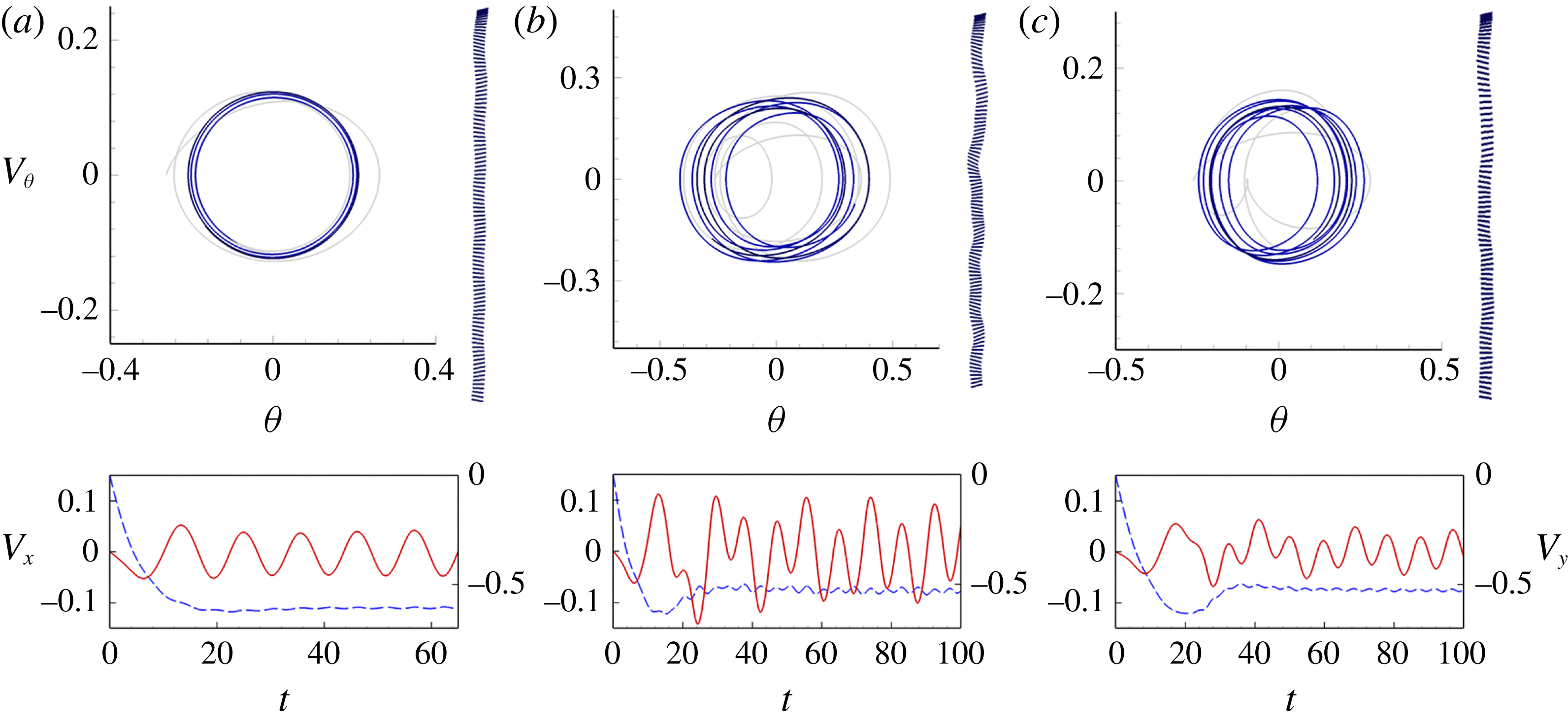
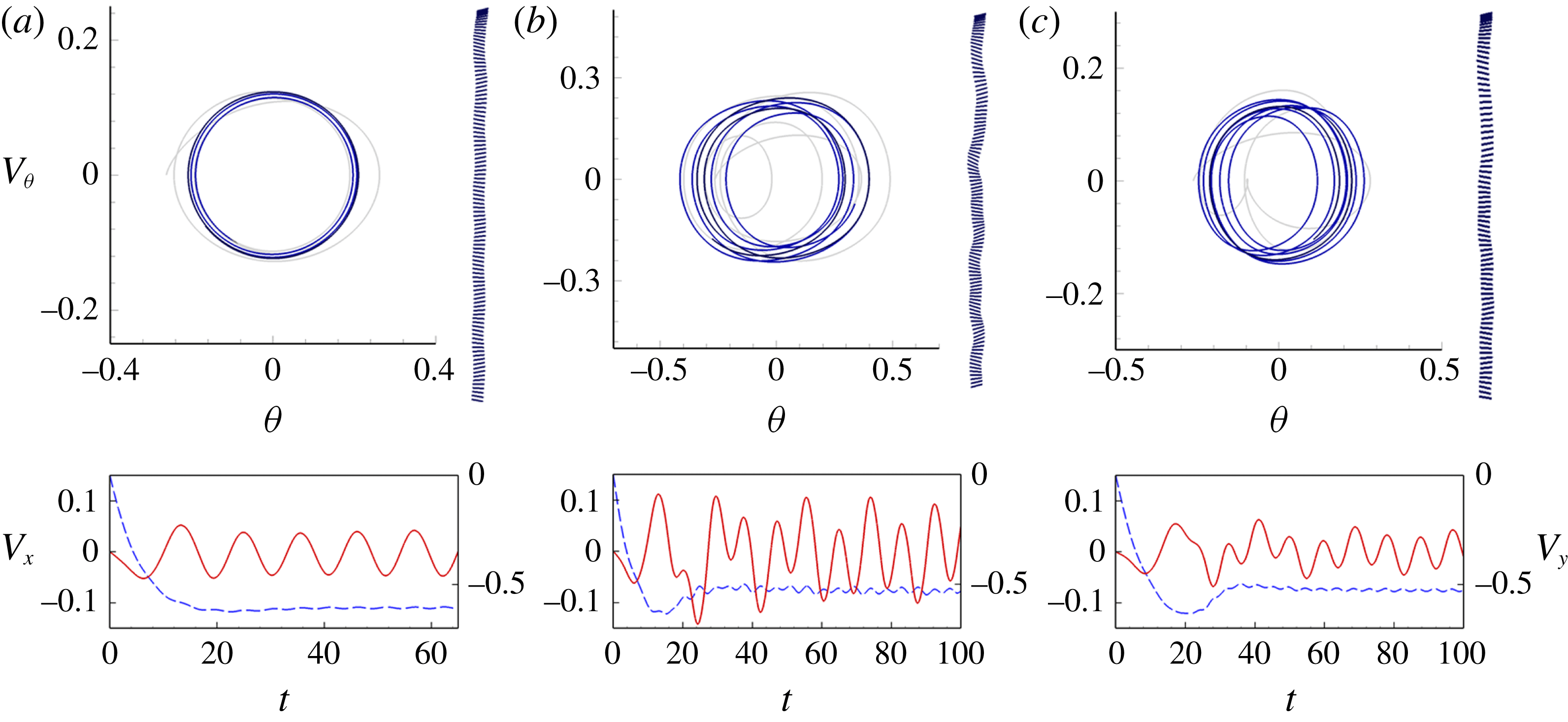
Reference Ern, Risso, Fabre and Magnaudet2012), the coupling interactions may cause the fall of a heavy plate to appear to be erratically wobbling. A plate shown in figure 4(c), maintains a clear stable vertical falling trajectory with small oscillations of
 $V_{x}$
and
 $V_{\unicode[STIX]{x1D703}}$
. When the
 $I^{\ast }$
is reduced in figure 4(b), the wobbling motion is significantly increased as the forces produced by the fluid structures yield greater effects. As
 $Re$
is reduced for figure 4(a), the frequency and pattern of oscillation become much more steady due to higher viscous effects. For the cases of periodic or erratic movement in figure 4, the downward rectilinear paths are restored by the gravitational force, as the motions circulate about the fixed point,
 $V_{\unicode[STIX]{x1D703}}=0$
and
 $\unicode[STIX]{x1D703}=0$
, of the phase portraits. Note that Horowitz & Williamson (Reference Horowitz and Williamson2010) separated the motion of rising or falling spheres into vibration (similar to flutter or wobble) and rectilinear (vertical fall) in the interest of investigating wakes and drag. Here, wobbling is distinguished from flutter in the interest of flight characteristics in terms of lift. These oscillations have a centre of rotation about the plate’s unit length, but generally not on the body. They generate very low lift and exhibit negligible flight characteristics in comparison to the fluttering seen for very light plates (figure 2
c). The present study follows Willmarth et al. (Reference Willmarth, Hawk and Harvey1964) and refers to wobbly rectilinear motions as stable falling.
Stable falling at
 $\unicode[STIX]{x1D703}_{0}=15^{\circ }$
showing how oscillations vary at (a)
 $Re=55$
and
 $I^{\ast }=3.0$
; (b)
 $Re=231$
and
 $I^{\ast }=3.0$
; (c)
 $Re=231$
and
 $I^{\ast }=5.0$
. Phase portraits are shown at the centre of each set, from light to dark through time. Trajectories are shown on the right side. Time histories at the bottom show
 $V_{x}$
in solid lines and
 $V_{y}$
in dashed lines.
3.2 Progression to tumble
The motions of the plates of
 $I^{\ast }=3.0$
and
 $5.0$
, and of
 $Re=80$
and
 $100$
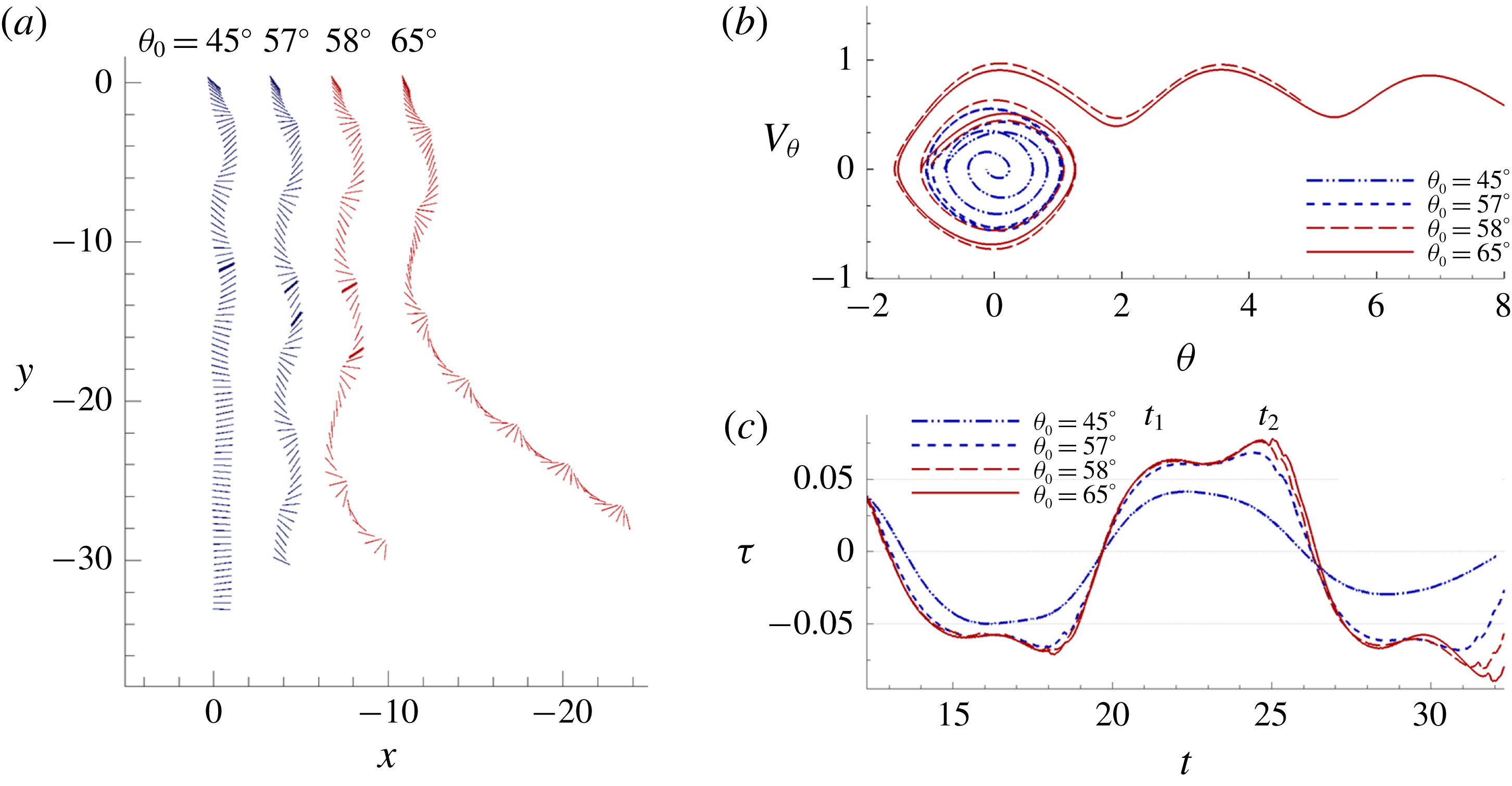
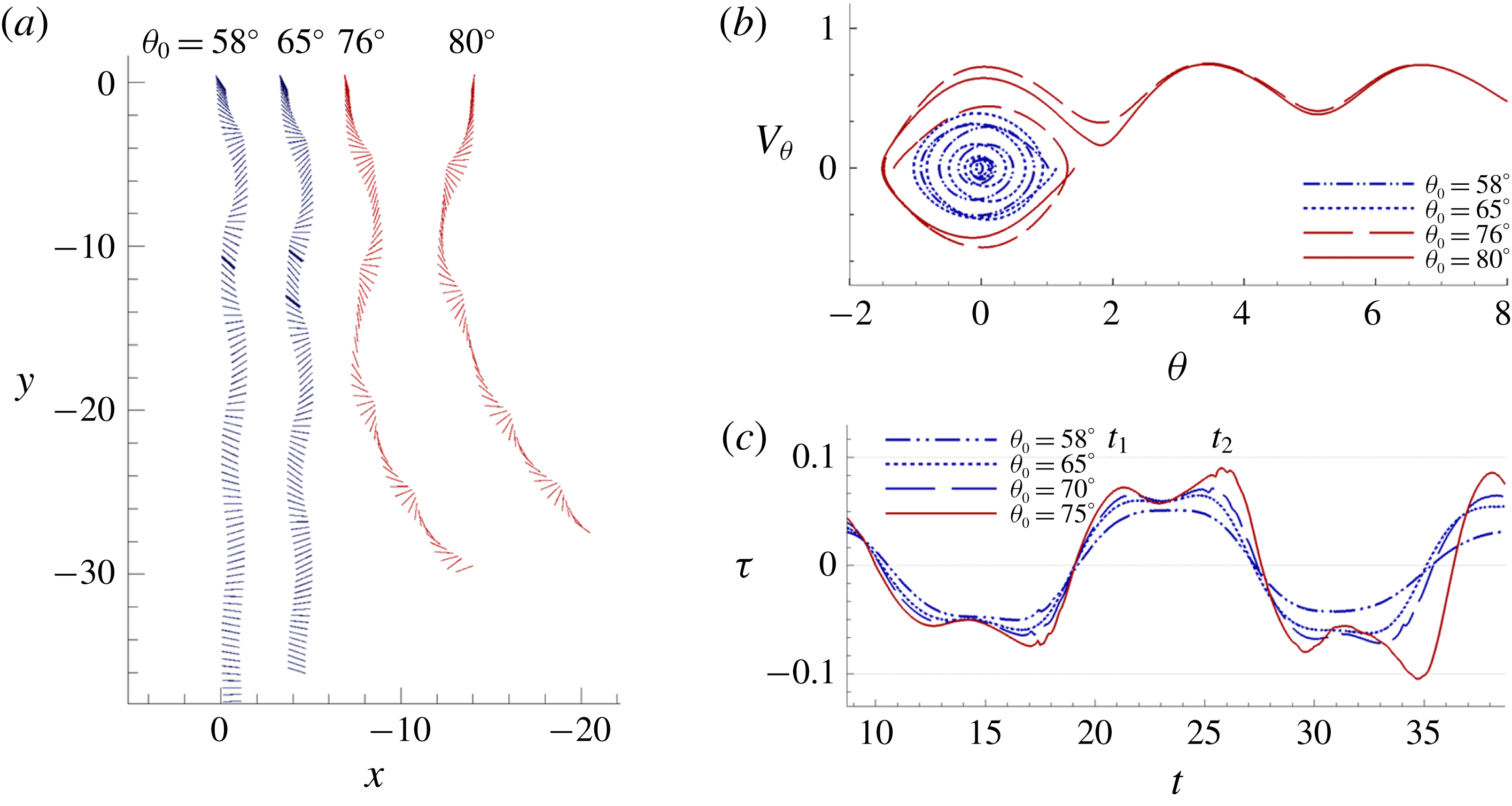
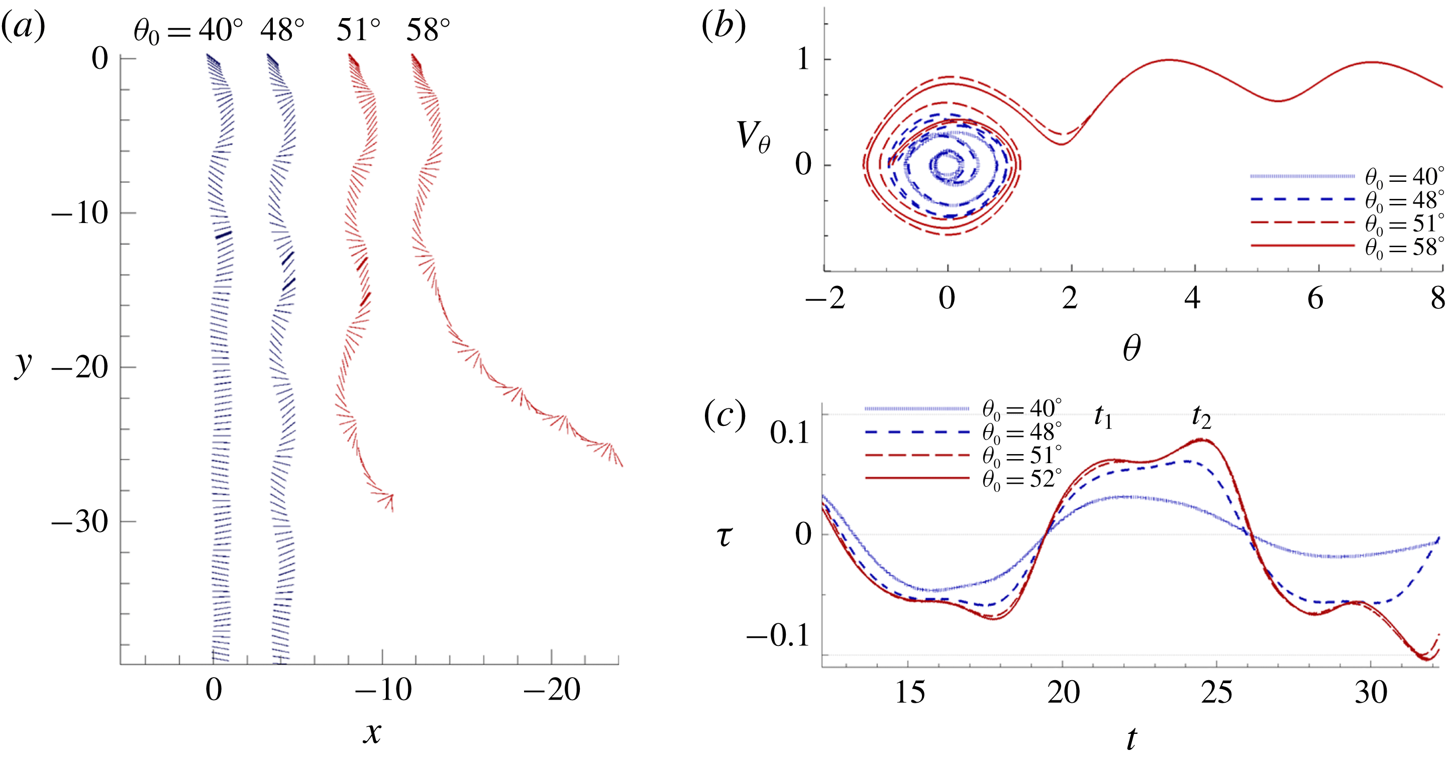
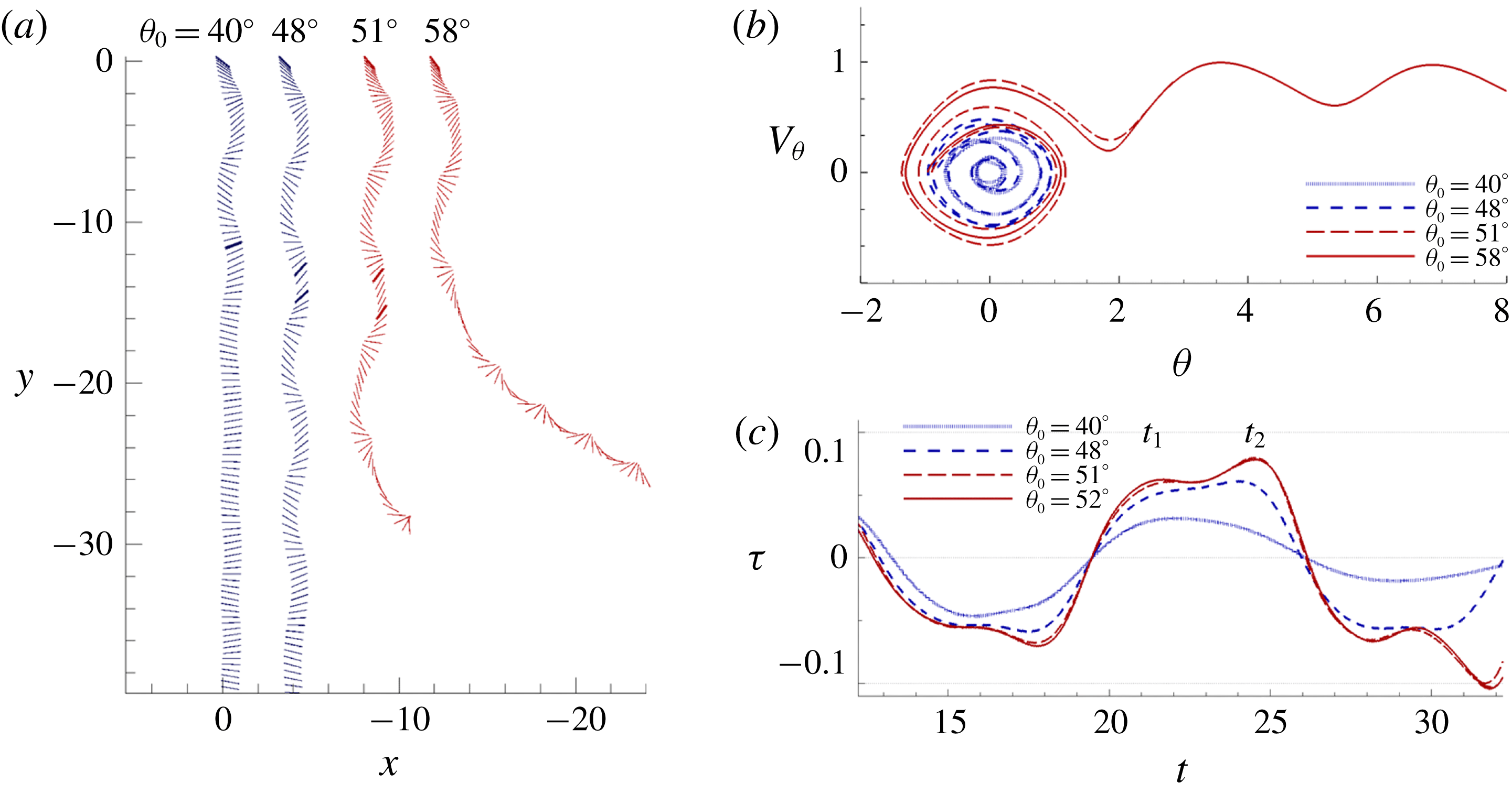
are shown in figures 5–7. It can be seen that plates increase their tendency to tumble at lower
 $I^{\ast }$
(comparing figure 5 with figure 6 at
 $\unicode[STIX]{x1D703}_{0}=65^{\circ }$
), or at higher
 $Re$
(comparing figure 5 with figure 7 at
 $\unicode[STIX]{x1D703}_{0}=58^{\circ }$
). The progression towards tumbling trajectories is illustrated in the phase portraits through the accumulation of angular velocity
 $V_{\unicode[STIX]{x1D703}}$
. Further decrease in
 $I^{\ast }$
or increase in
 $Re$
results in successively greater rotating oscillation through each turning point, toppling the plates sooner into tumble. The three sets of figures also show that the duration towards either stable falling or tumbling are considerably longer for heavier plates, for which the spatial domain required may be of the order of
 $10^{2}$
of the chord length from dynamical models (Hu & Wang Reference Hu and Wang2014). Dynamical phase portraits from figures 5(b) to 7(b) illustrate clearly how the trajectories divert. Stable falling plates scroll inward, approaching the theoretical fixed point; tumbling plates progressively spiral outwards, away from the fixed point, and eventually topple over
 $\unicode[STIX]{x1D703}=90^{\circ }$
towards periodic limit cycles.
Development towards the two bistable flight states at
 $Re=80$
and
 $I^{\ast }=3.0$
at various
 $\unicode[STIX]{x1D703}_{0}$
: (a) the trajectories; (b) phase portraits of
 $\unicode[STIX]{x1D703}$
and
 $V_{\unicode[STIX]{x1D703}}$
; (c) time histories of torque. The torque peaks at times
 $t_{1}$
and
 $t_{2}$
are shown in bold in (a).
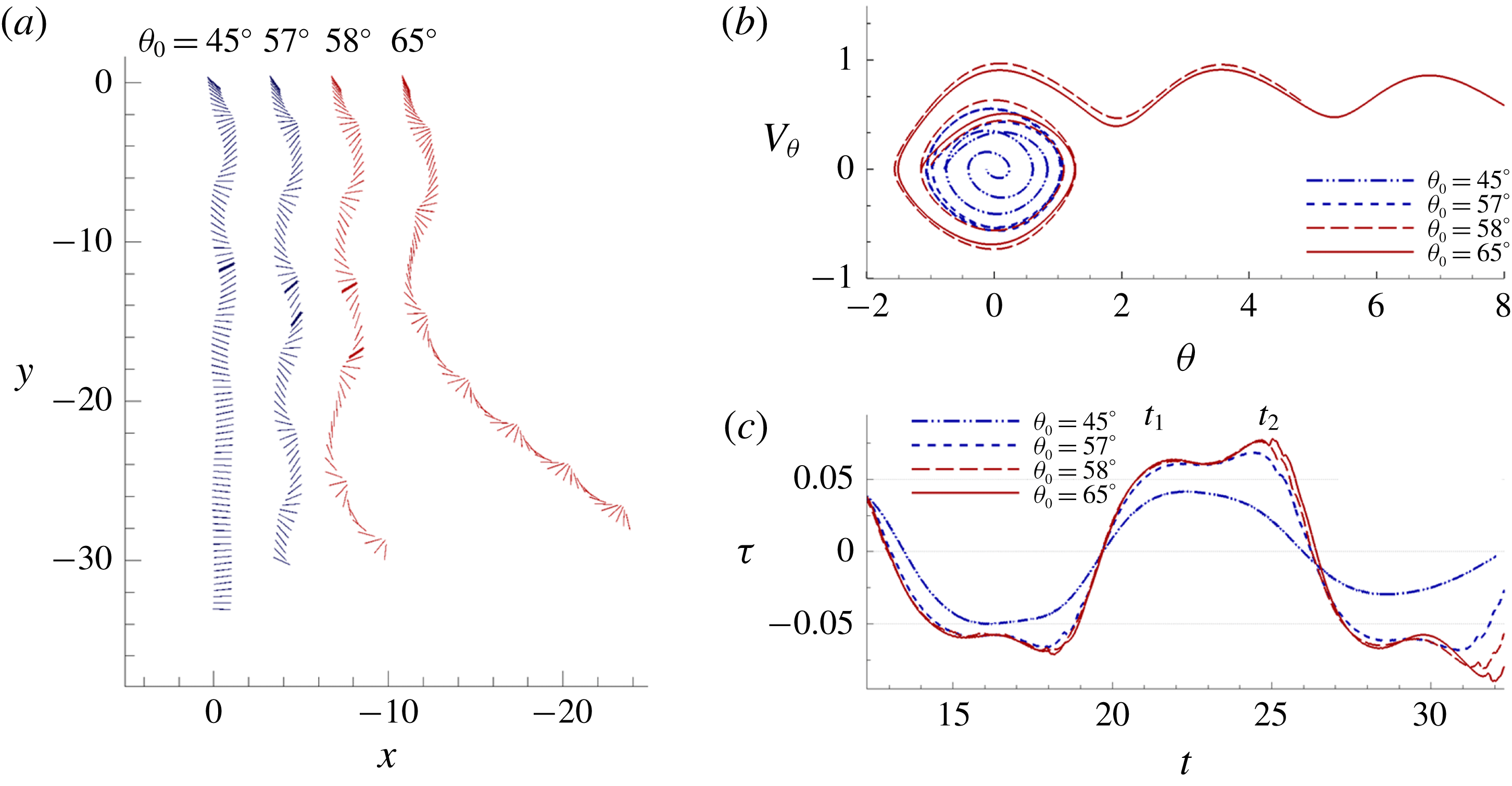
Development towards the two bistable flight states at
 $Re=80$
and
 $I^{\ast }=5.0$
at various
 $\unicode[STIX]{x1D703}_{0}$
: (a) the trajectories; (b) phase portraits of
 $\unicode[STIX]{x1D703}$
and
 $V_{\unicode[STIX]{x1D703}}$
; (c) time histories of torque. The torque peaks at times
 $t_{1}$
and
 $t_{2}$
are shown in bold in (a).

Development towards the two bistable flight states at
 $Re=100$
and
 $I^{\ast }=3.0$
at various
 $\unicode[STIX]{x1D703}_{0}$
: (a) the trajectories; (b) phase portraits of
 $\unicode[STIX]{x1D703}$
and
 $V_{\unicode[STIX]{x1D703}}$
; (c) time histories of torque. The torque peaks at times
 $t_{1}$
and
 $t_{2}$
are shown in bold in (a).
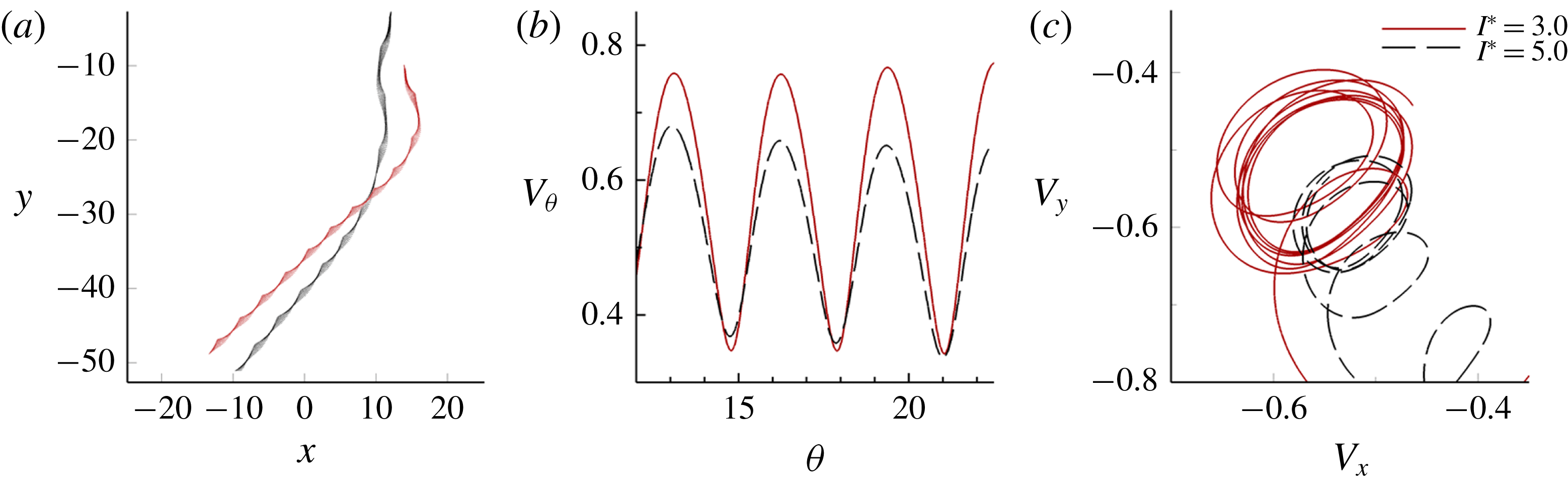
Comparison of two tumbling plates with
 $I^{\ast }=3.0$
and
 $5.0$
, at
 $Re=80$
and
 $\unicode[STIX]{x1D703}_{0}=75^{\circ }$
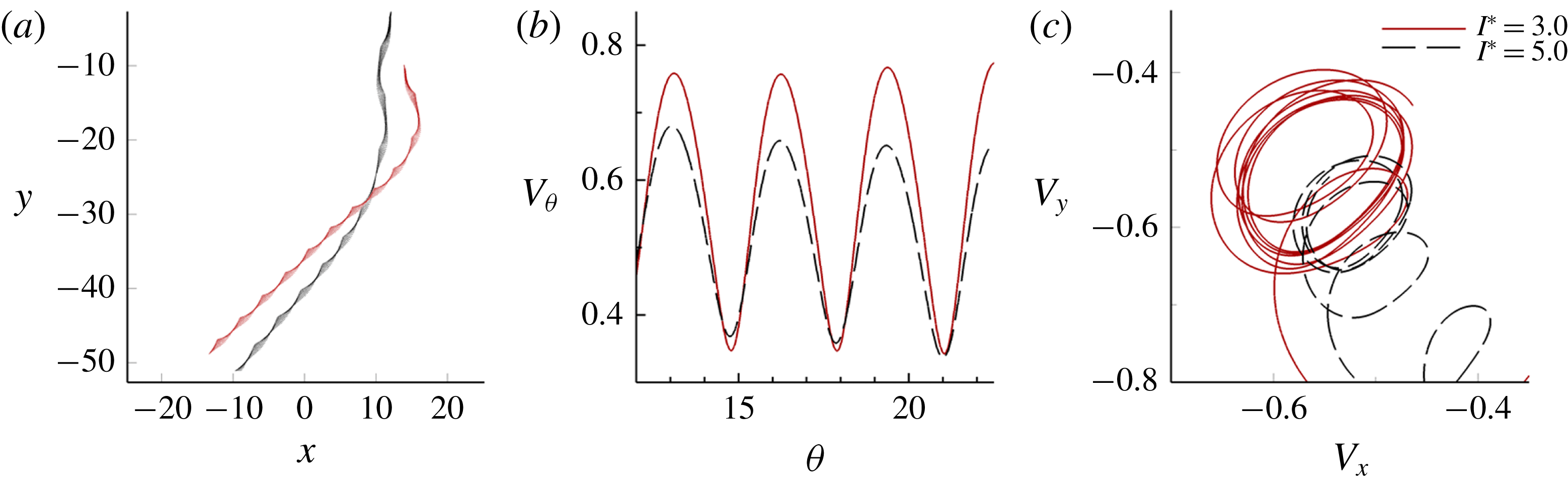
: (a) trajectories; (b) angular phase portrait; (c) linear phase portrait.
Velocities and descent angles during steady tumbling flights at various
 $I^{\ast }$
and
 $Re$
released at
 $\unicode[STIX]{x1D703}_{0}=75^{\circ }$
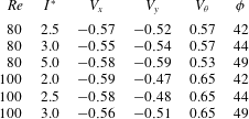
. All are average values are calculated after the plates have reached steady state decent.
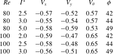
Corresponding to the discussion on stable falling in § 3.1, figure 8(a) illustrates the behaviour of tumbling flight for different configurations. Table 2 collectively presents the changes in tumbling performance for different
 $I^{\ast }$
and
 $Re$
. It is expected that some differences in velocities would occur due to the difference in limit cycles. Indeed, this is first shown by the increase in the descent angle,
 $\unicode[STIX]{x1D719}$
, with respect to the horizontal axis when
 $I^{\ast }$
increases, as per figure 8(a). This is attributed to the increase of the vertical velocity
 $V_{y}$
, and the decrease of
 $V_{\unicode[STIX]{x1D703}}$
and
 $V_{x}$
, illustrated in figure 8(b,c). The effect is similar to the findings of Dupleich (Reference Dupleich1941) and Wang et al. (Reference Wang, Hu, Xu and Wu2013), where the descent angle is increased with wing loading. At higher
 $Re$
, velocities experience larger fluctuations, rendering the limit cycles and their changes less obvious. The cases of
 $Re=100$
from table 2 achieve noticeably higher rotational speeds as they are subjected to less viscous drag, while the descent angle
 $\unicode[STIX]{x1D719}$
remains the same as those of
 $Re=80$
.
3.3 Bistability
An important feature of figures 5–7 is the dependence of the flight states on the initial angles,
 $\unicode[STIX]{x1D703}_{0}$
. This dependence sets the transition state from stable falling to tumbling, apart from the conventional flight regimes found in figure 3, where the trajectories of tumbling and fluttering are invariant with the initial conditions (Andersen et al.
Reference Andersen, Pesavento and Wang2005b
; Wan et al.
Reference Wan, Dong and Liang2012; Wu & Lin Reference Wu and Lin2015).
By extending the analyses of trajectories and phase portraits in § 3.2 to the simulations across the range of
 $I^{\ast }$
and
 $Re$
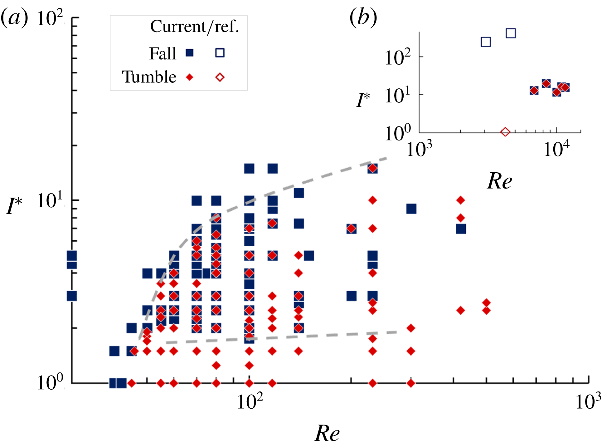
in figure 9 for heavy plates of nominal thickness, i.e.
 $h^{\ast }=1/128$
, the bistability region is mapped thoroughly. Beyond the upper boundary, plates will not tumble at any
 $\unicode[STIX]{x1D703}_{0}$
; and below the lower boundary, plates will develop into tumble and will not steadily fall. From the mapping at low
 $Re$
, the region of high viscosity stable falling at
 $Re<50$
connects with the stable falling state. This region is dominated by fluid resistance and the gravitational effect. The bistable region with tumbling grows rapidly from
 $Re$
of 50 to 70 as the effect of flow inertia becomes significant. This effect is moderated from
 $Re>80$
and steadily expands the bistable region for heavier plates to tumbling at higher Reynolds numbers.
Map of flight states for heavy rectangular plates of nominal thickness, showing the region of bistability: (a) current numerical results; (b) current experiment and reference (Heisinger et al. Reference Heisinger, Newton and Kanso2014) data. The upper and lower boundaries of the bistable region are demarcated by dashed lines.

Relationship between the critical initial angle
 $\unicode[STIX]{x1D703}_{0cr}$
(deg) and (a)
 $I^{\ast }$
; (b)
 $Re$
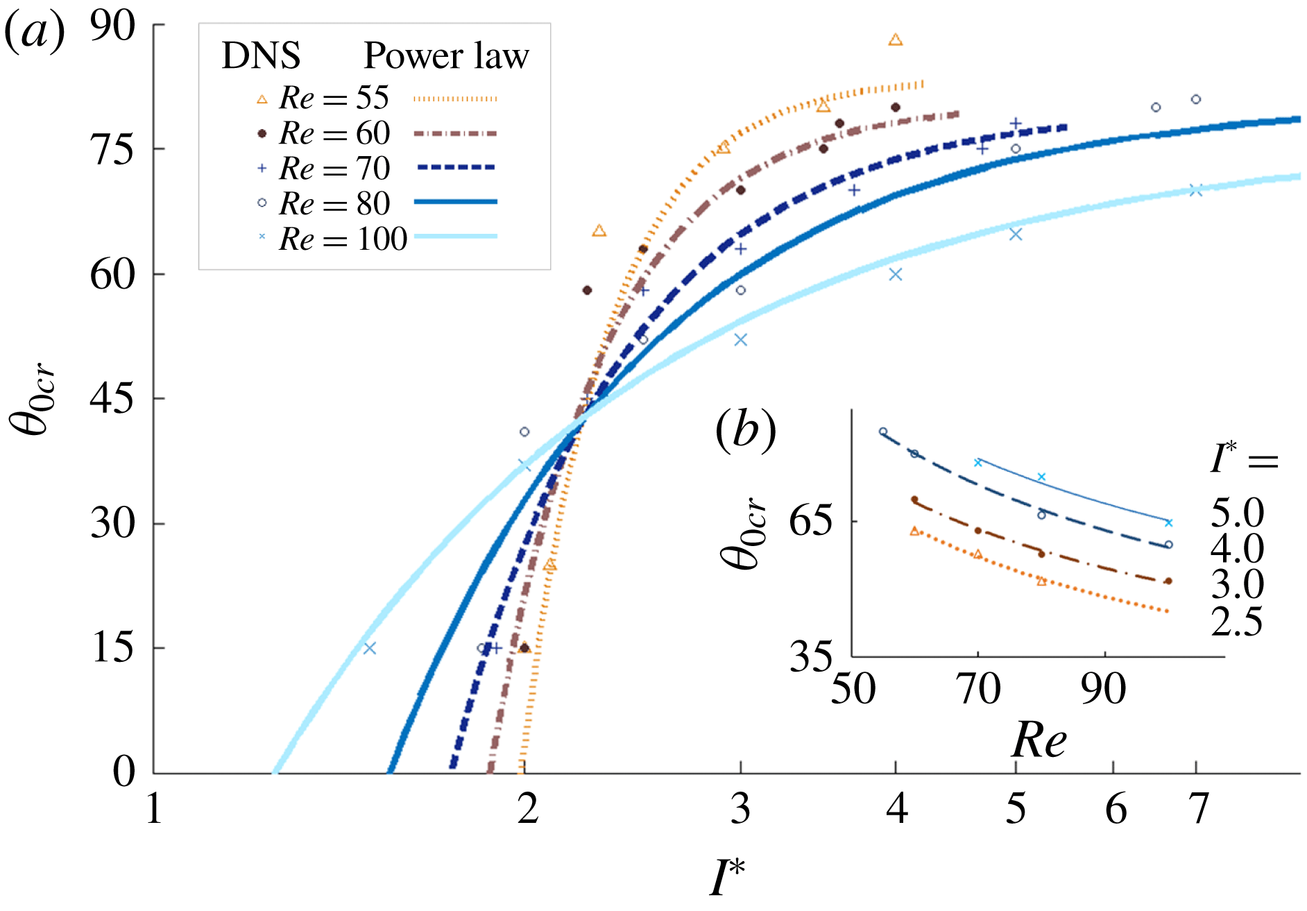
for heavy rectangular plates of nominal thickness. DNS results are shown by the data points; power laws are shown by the lines.

To elucidate the relationships among
 $I^{\ast }$
,
 $Re$
and
 $\unicode[STIX]{x1D703}_{0}$
, focus is turned to determining the critical angle
 $\unicode[STIX]{x1D703}_{0cr}$
that sets apart stable falling from tumbling trajectories for a given
 $I^{\ast }$
of the plate, and
 $Re$
of the fluid. As illustrated in figure 10(a), a steeper initial angle
 $\unicode[STIX]{x1D703}_{0cr}$
is required to initiate tumble for heavier plates. This is also true for more viscous fluids. The lower the
 $Re$
, the more abrupt the change of
 $\unicode[STIX]{x1D703}_{0cr}$
. In general, for each
 $Re$
in figure 10(a), simulation data suggest a region of sharp change of
 $\unicode[STIX]{x1D703}_{0cr}$
, followed by a region of smaller changes as
 $I^{\ast }$
increases. At one extreme end with small
 $I^{\ast }$
, where the viscous effect dominates, plates will tumble independent of
 $\unicode[STIX]{x1D703}_{0}$
. The data should then meet the positive
 $I^{\ast }$
axis. At the other end of the axis as
 $I^{\ast }\sim \infty$
, where the inertial effect dominates, tumbling should cease as plates will fall flat. The power law
 $k=c_{1}I^{\ast c_{2}}$
is fitted to reflect these changes at different Reynolds numbers. A similar fit is also applied to figure 10(b) as
 $\unicode[STIX]{x1D703}_{0cr}=kRe^{c_{3}}$
for various
 $I^{\ast }$
. Interestingly, data intersect at a neutral point and separate the two regions at approximately
 $\unicode[STIX]{x1D703}_{0cr}\approx 45^{\circ }$
and
 $I^{\ast }\approx 2$
for all Reynolds numbers under study. The combined power law thus abridges the viscous and inertial scales:
 $$\begin{eqnarray}\displaystyle \unicode[STIX]{x1D703}_{0cr}=c_{1}I^{\ast c_{2}}Re^{c_{3}}. & & \displaystyle\end{eqnarray}$$
The coefficients can be obtained by the method of least squares, i.e.
 $c_{1}=580$
,
 $c_{2}=0.49$
and
 $c_{3}=-0.65$
. Equation (3.1) serves as a simple expression that holds well for
 $I^{\ast }>2.5$
with a mean error of 5 %. At
 $I^{\ast }<2.5$
, the term
 $c_{2}$
should be close to zero near the neutral point. The critical initial angles
 $\unicode[STIX]{x1D703}_{0cr}$
for cases in figures 5–7 are
 $58^{\circ }$
,
 $75^{\circ }$
and
 $51^{\circ }$
, respectively. Note that the relationship changes upon variation of
 $h^{\ast }$
; refer to § 3.6.
The works by Field et al. (Reference Field, Klaus and Moore1997) and Wu & Lin (Reference Wu and Lin2015) hinted at a higher initial (or previous) angle
 $\unicode[STIX]{x1D703}_{0}$
result with an increase of
 $\unicode[STIX]{x1D703}$
at turn points. However, the rate of increase of
 $\unicode[STIX]{x1D703}$
is lower than the increase of
 $\unicode[STIX]{x1D703}_{0}$
for their study of lighter plates. Whereas, within the bistable regime,
 $\unicode[STIX]{x1D703}$
is increased at subsequent turns for plates developing into tumble. The falling problem may therefore be perceived as the presence of multiple limit cycles within the FSI system, and whether the solid can kinematically escape from one and into another. In the case of chaotic motion, the solid may undergo interchange of limit cycles under the build up and dissipation of velocities. Observing the phase portraits from figures 5(b) to 7(b), when an initial angle is brought close to
 $\unicode[STIX]{x1D703}_{0cr}$
, the trajectories are changed very abruptly. A plate travelling with sufficient
 $V_{x}$
and
 $V_{y}$
to the turning point does not maintain itself near
 $\unicode[STIX]{x1D703}_{0}=90^{\circ }$
, and is ‘deflected’ at this dynamical saddle point. Plates of different
 $\unicode[STIX]{x1D703}_{0}$
behave the same and converge to identical tumbling limit cycles as the dynamical systems remain unchanged (conjugate trajectory is plotted in the same direction for clarity). The change of
 $\unicode[STIX]{x1D703}_{0}$
affects flight state by changing the attraction basin of the dynamic system (Chrust et al.
Reference Chrust, Bouchet and Dušek2013), displacing it from the proximity of one attractor towards another. In general, sufficient input of velocity
 $V_{x}$
,
 $V_{y}$
or
 $V_{\unicode[STIX]{x1D703}}$
in a specific instance may also alter the flight pattern (results not shown here), like a swaying leaf rolling into tumble under a sudden gust of wind.
3.4 Experimental observation
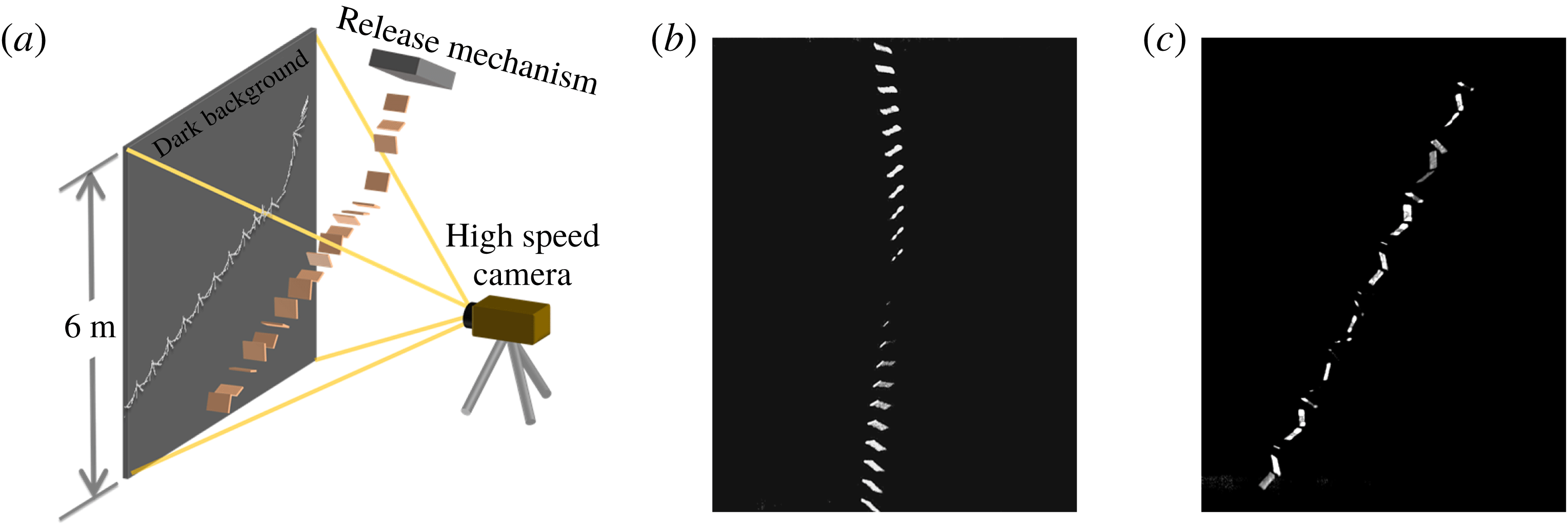
(a) Schematic of the experimental set-up; superimposed snapshots for
 $Re=10\,900$
,
 $I^{\ast }=16.3$
at (b)
 $\unicode[STIX]{x1D703}_{0}=45^{\circ }$
and (c)
 $\unicode[STIX]{x1D703}_{0}=75^{\circ }$
.

To confirm the finding of bistability and its dependence on
 $\unicode[STIX]{x1D703}_{0}$
, an experiment is conducted to record trajectories of plastic and paper cards freely falling in air. A drop length of six metres is provided, equivalent to a DNS vertical domain of
 $O(10^{2})$
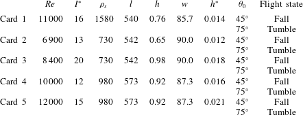
chord lengths. Figure 11(a) shows a schematic of the experimental set-up. Each release is kept consistent; the initial angle
 $\unicode[STIX]{x1D703}_{0}$
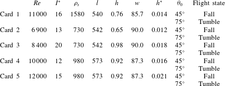
as well as the two-dimensionality of the trajectory are carefully controlled. The properties of the falling cards are listed in table 3. The specimens move through air freely. The motions are captured with a Phantom V9.1 high speed camera calibrated to frames of the stable falling and tumbling trajectories of the light-coloured plates in front of a dark background provided. Two initial angles are tested for each card, as shown in figure 11(b–c).
Figure 11(b) is a time overlap of a card released at
 $\unicode[STIX]{x1D703}_{0}=45^{\circ }$
in stable falling through the time instances captured. Its trajectory bears resemblance to the stable falling trajectories found in figures 5(a) to 7(a). The tumbling flights, resulting from the steep angle of
 $\unicode[STIX]{x1D703}_{0}=75^{\circ }$
, as seen in figure 11(c), have a rather steep angle of descent
 $\unicode[STIX]{x1D719}\approx 60^{\circ }$
. This angle is in agreement with previous experimental findings in relation to the card’s aspect ratio (Wang et al.
Reference Wang, Hu, Xu and Wu2013). Aspect ratios are kept small to maintain spanwise rigidity. The consequence of this is the apparent three-dimensional flow effect such that portions of the circulation and lift effects would escape through the span and may reduce the tendency to tumble (see § 3.5). Table 3 provides a list of results and corresponding parameters which are added to the map of flight states in figure 9(b). The experimental results lie clearly within the findings from falling disks (Heisinger et al.
Reference Heisinger, Newton and Kanso2014), and are in the vicinity of the bistable boundaries from low Reynolds numbers. Increasing thickness of the plate would promote tumble, as per the DNS findings provided in figure 20. Under the circumstances of thickness and aspect ratio, the critical angles for flight states would be below the prediction made by (3.1).
Experimental parameters and flight states corresponding to different initial angles
 $\unicode[STIX]{x1D703}_{0}$
. Properties of specimen in terms of density
 $\unicode[STIX]{x1D70C}_{s}$
(
 $\text{kg}~\text{m}^{-3}$
), length
 $l$
(mm), thickness
 $h$
(mm) and span width
 $w$
(mm).
3.5 Flow fields
The discussion turns to exploring the physical mechanism that leads to the bistability of flight states by capturing the flow dynamics that leads to the divergence in velocities from stable falling to tumbling. It can be seen from figures 5(c) to 7(c) that the rotating plates in developing their flight paths generally see two increases in
 $\unicode[STIX]{x1D70F}$
at
 $t_{1}$
and
 $t_{2}$
. In particular, figure 5(c) suggests that
 $\unicode[STIX]{x1D70F}$
at
 $t_{2}$
provides a step increase from stable falling at
 $\unicode[STIX]{x1D703}_{0}=57.0^{\circ }$
to tumbling at
 $58.0^{\circ }$
. Additionally, the case at
 $57.0^{\circ }$
that settles towards stable falling shows that the build up of
 $\unicode[STIX]{x1D70F}$
at
 $t_{2}$
is not caused by the tendency to tumble itself.
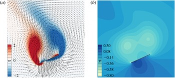
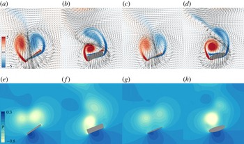
Flow fields around a stable falling plate at
 $Re=80$
,
 $I^{\ast }=3$
and
 $\unicode[STIX]{x1D703}_{0}=45^{\circ }$
at
 $t_{1}$
per figure 5: (a) vorticity and velocity fields; (b) pressure field.

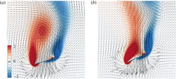
Vorticity and velocity fields at
 $t_{2}$
per figure 5, at
 $Re=80$
and
 $I^{\ast }=3$
: (a)
 $\unicode[STIX]{x1D703}_{0}=45^{\circ }$
; (b)
 $\unicode[STIX]{x1D703}_{0}=58^{\circ }$
.

Attention is thus turned to the development of torque. The instantaneous field of vorticity, defined as
 $\unicode[STIX]{x1D714}=\unicode[STIX]{x2202}u/\unicode[STIX]{x2202}y-\unicode[STIX]{x2202}v/\unicode[STIX]{x2202}x$
and which is positive for clockwise rotation, are similar between the instants
 $t_{1}$
and
 $t_{2}$
, as shown in figures 12(a) and 13(a). In figure 13(a), the movement sheds a vortex (red) along the tip of the leading edge, whereas in figure 13(b), it curls behind the plate causing a bias in the flow field. The bias asserts an increase in torque, causing a maximum at
 $t_{2}$
with the flow momentum, as seen in figure 5(c).
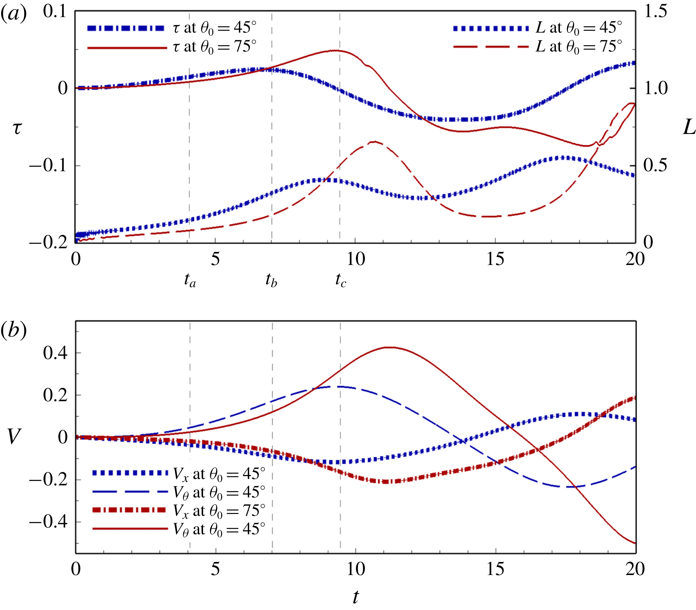
Time histories of (a) torque and lift, and (b) angular velocity histories for the case of
 $Re=80$
,
 $I^{\ast }=5.0$
, at
 $\unicode[STIX]{x1D703}_{0}=45^{\circ }$
stable falling and
 $\unicode[STIX]{x1D703}_{0}=75^{\circ }$
tumbling. Time steps
 $t_{a}$
,
 $t_{b}$
and
 $t_{c}$
correspond to the separate instants in figures 15 and 16.

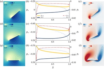
Sets of pressure contours (a,d,g), the distributions of normal and shear stresses on the upper and lower surfaces of the plate (b,e,h) and velocity fields with vorticity contours (c,f,i). Each row corresponds to the initial instances,
 $t_{a}$
,
 $t_{b}$
and
 $t_{c}$
in figure 14, of stable falling at
 $Re=80$
,
 $I^{\ast }=5.0$
and
 $\unicode[STIX]{x1D703}_{0}=45^{\circ }$
.

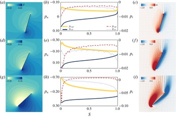
Sets of pressure contours (a,d,g), the distributions of normal and shear stresses on the upper and lower surfaces of the plate (b,e,h) and velocity fields with vorticity contours (c,f,i). Each row corresponds to the initial instances,
 $t_{a}$
,
 $t_{b}$
and
 $t_{c}$
in figure 14, of tumbling at
 $Re=80$
,
 $I^{\ast }=5.0$
and
 $\unicode[STIX]{x1D703}_{0}=75^{\circ }$
.

Investigation returns to the initial stage of falling and the respective formation of flow structures. The evolution of the plate’s dynamics is analysed through three instances,
 $t_{a}$
,
 $t_{b}$
and
 $t_{c}$
, identified in figure 14, where the cases of falling and tumbling are compared. At
 $t_{a}$
, the stable falling plate at a smaller
 $\unicode[STIX]{x1D703}_{0}=45^{\circ }$
begins with greater initial forces and torque than the case of tumbling at
 $\unicode[STIX]{x1D703}_{0}=75^{\circ }$
as seen in figure 14(a). The lift is caused by the large pressure difference between the surfaces due to the flow resistance to falling, illustrated in figure 15(a). The respective pressures of the upper and lower surfaces are shown in figure 15(b). This stable falling case stands in sharp contrast to the tumbling plate, where a smaller pressure field takes form, as shown in figure 16(a,b). During this time, the vortices have been formed at the leading and trailing edges for figure 15(b,c). This is also noted by the surface shear stress
 $p_{t}=(\unicode[STIX]{x1D70C}_{f}V_{\infty }^{2}/Re)(\unicode[STIX]{x2202}u^{\prime }/\unicode[STIX]{x2202}y^{\prime })$
with ‘primes’ denoting the local frame of reference. As a result of the vortex system, a recirculating flow between the vortex pair of the leading and trailing edges takes hold, pushing uniformly on the plate similar to figure 13(a). Meanwhile, the tumbling case in figure 16(b) develops contours similar to a classic airfoil as it falls through the fluid at a steep angle.
At the instant
 $t_{b}$
, the pressure difference moves closer to the centre of mass in figure 15(d) as the vortices at the tips begin to grow and elongate, forming a relatively uniform distribution recirculating flow velocity over and along the upper surface in figure 15(e,f). Both effects cause the torque
 $\unicode[STIX]{x1D70F}$
of the stable falling plate to begin to decrease after reaching its peak in figure 14(a,b). This leads to a much smaller
 $V_{\unicode[STIX]{x1D703}}$
for the falling plate with the peak between
 $t_{b}$
and
 $t_{c}$
. Although the tumbling plate experiences smaller pressure fields at
 $t_{b}$
, the large pressure difference forward of the plate produces a lift-induced torque about the centre of mass, as per figure 16(e,f).
As the plate reaches
 $t_{c}$
, the stable falling plate has significantly slowed down, with the lower surface confronting the vertical fall and forming a large pressure difference distributed along the chord in figure 15(g,h). According to figure 14(a,b),
 $\unicode[STIX]{x1D70F}$
has now changed orientation and the plate eventually seesaws backwards, diminishing its rotation. Meanwhile, the tumbling plate continues to increases its velocities, pressure and local lift, thereby propelling its torque to a much higher value than its stable falling counterpart. Its
 $\unicode[STIX]{x1D70F}$
eventually allows the plate to tumble. At the same time, the leading and trailing edge vortices form a system on the upper surface that confines the recirculating flow to the right of the plate and provides further torque in the manner described in figure 13(b). Observing the two cases at the same angle in figures 15(a,b) and 16(g,h), the case of
 $\unicode[STIX]{x1D703}_{0}=75^{\circ }$
has already accumulated a larger magnitude of pressure difference at the leading edge. This is attributed to the difference in lift between the falling and tumbling plates.
It is of further interest to investigate how the lift sets the trajectories onto separate courses. Recall that the instance of free fall from a steep initial angle in figure 16(a) is an airfoil in a free stream at initially low angle of attack
 $\unicode[STIX]{x1D6FC}$
as per figure 2(a). The leading edge vortex produces a lift acting through the centre of pressure, at a moment arm about the plate’s centre of mass (Smith Reference Smith1971). The plate follows the conventional lift curve as
 $\text{d}L/\text{d}\unicode[STIX]{x1D6FC}>0$
with a positive correlation between
 $L$
and
 $\unicode[STIX]{x1D6FC}$
. The torque induced is responsible for the arcing trajectory as well as the development of
 $V_{\unicode[STIX]{x1D703}}$
towards tumble. On the other hand, the lift mildly decreases beyond the stall angle
 $\unicode[STIX]{x1D6FC}_{stall}$
between
 $20^{\circ }$
and
 $40^{\circ }$
as
 $\text{d}L/\text{d}\unicode[STIX]{x1D6FC}<0$
for low
 $Re$
flows (Sun & Boyd Reference Sun and Boyd2004; Okamoto & Azuma Reference Okamoto and Azuma2011). This relates to the behaviour of the stable falling plate in figure 15(a), where the lift is reduced at an increasing
 $\unicode[STIX]{x1D6FC}$
. The static case of
 $\unicode[STIX]{x1D6FC}_{stall}$
can thus be seen as closely related to
 $\unicode[STIX]{x1D703}_{0cr}$
in unsteady free fall.
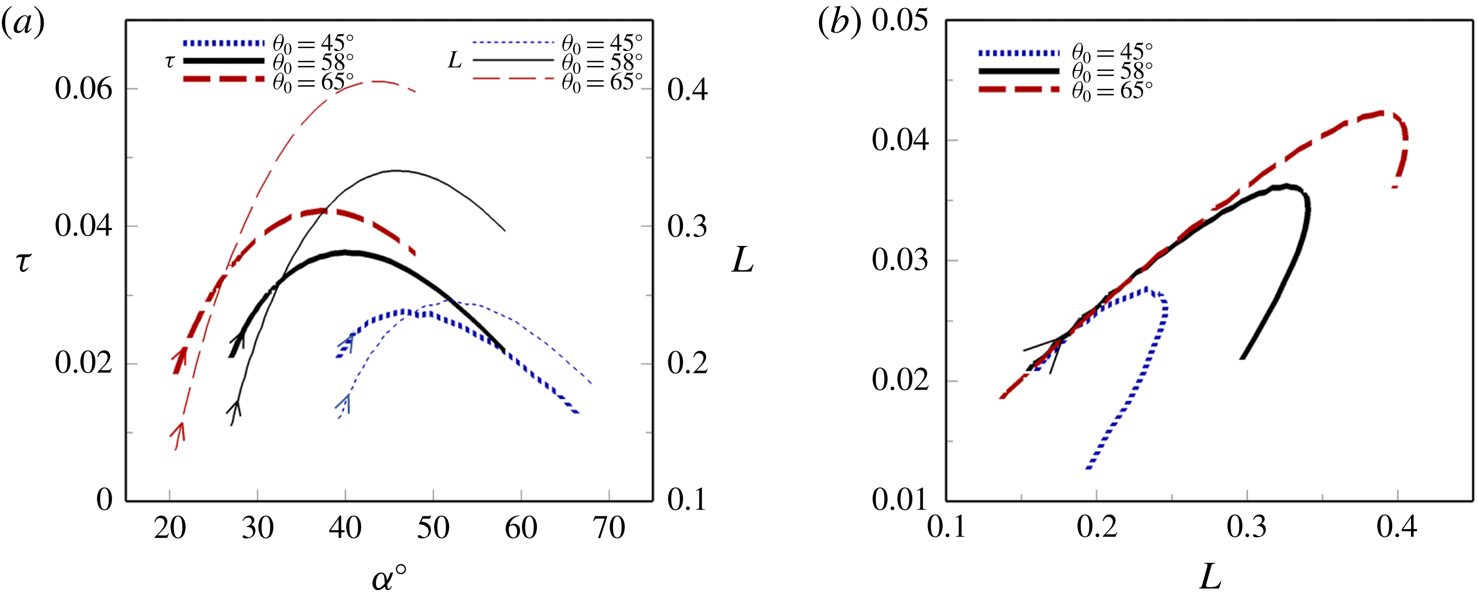
Based on the above knowledge, lift curves through the initial stages of the drops are drawn in figure 17(a) for three simulations: stable falling, critical angle and tumbling. Due to the unsteady increase in
 $\boldsymbol{V}$
and the development of vortices in free fall, all cases initially have increasing
 $L$
as they take flight. Looking closely, the two cases launched at steeper
 $\unicode[STIX]{x1D703}_{0}$
reside on the left of figure 17(a), attaining higher
 $L$
with a greater slope at lower
 $\unicode[STIX]{x1D6FC}$
. The stable falling case resides on the right side. The lift-generated torque curves behave similarly in figure 17(a). Figure 17(b) shows the evolution of
 $\unicode[STIX]{x1D70F}$
versus
 $L$
, exhibiting linear increases, and extending longer for higher
 $\unicode[STIX]{x1D703}_{0}$
, sufficient for the plate to tumble where
 $\unicode[STIX]{x1D703}_{0}\geqslant \unicode[STIX]{x1D703}_{0cr}$
. Interestingly,
 $\unicode[STIX]{x1D70F}$
‘boomerangs’ back with the decrease of
 $L$
and
 $\boldsymbol{V}$
approaching the turn point. In general, when the plate traverses in smaller arcs, rotational stability is predominately driven by unsteady fluid effects (Paidoussis et al.
Reference Paidoussis, Price and Langre2011). The addition of a rotational lift term to the dynamic model by Pesavento & Wang (Reference Pesavento and Wang2004) has a similar effect.
Initial stage of falling for
 $Re=80$
,
 $I^{\ast }=3.0$
when steadily falling at
 $\unicode[STIX]{x1D703}_{0}=45^{\circ }$
, tumbling at
 $\unicode[STIX]{x1D703}_{0cr}=58^{\circ }$
and tumbling at
 $\unicode[STIX]{x1D703}_{0}=75^{\circ }$
: (a)
 $\unicode[STIX]{x1D70F}$
and
 $L$
versus
 $\unicode[STIX]{x1D6FC}$
(deg); (b)
 $\unicode[STIX]{x1D70F}$
versus
 $L$
. The arrows indicate the direction of time.

(a) Variations of
 $\unicode[STIX]{x1D70F}_{max}$
experienced by plates of different
 $I^{\ast }$
and
 $Re$
with
 $\unicode[STIX]{x1D703}_{0}$
. Symbols are solid filled at
 $\unicode[STIX]{x1D703}_{0cr}$
. Dashed lines denote the slopes. For stable falling plates, i.e. at low
 $\unicode[STIX]{x1D703}_{0}$
,
 $\unicode[STIX]{x1D70F}_{max}$
occurs typically in the first period of oscillation. For tumbling plates,
 $\unicode[STIX]{x1D70F}_{max}$
is recorded prior to the onset of tumbling. (b) The associated maximum angular acceleration,
 $\text{d}V_{\unicode[STIX]{x1D703}}/\text{d}t$
.

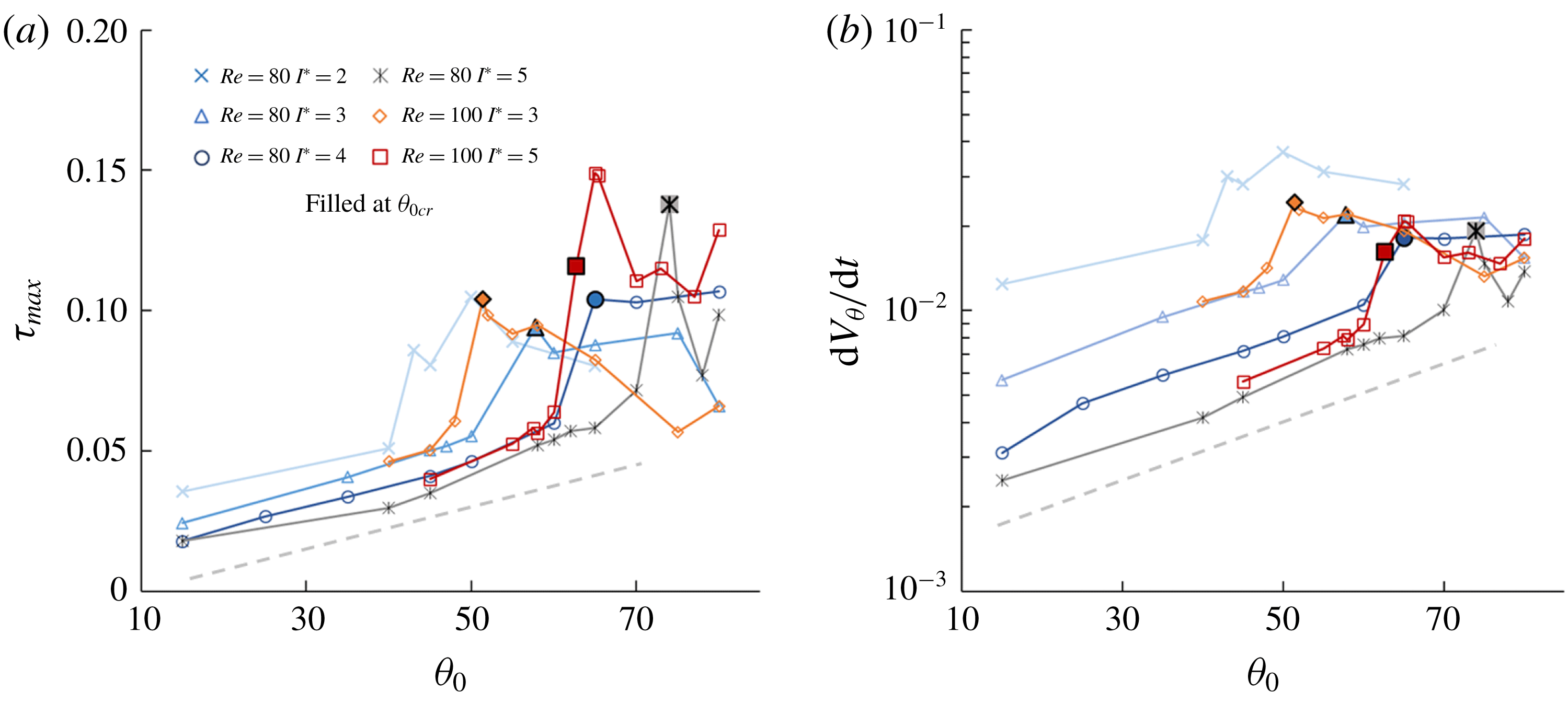
From the increase in torque at the initial stage of tumbling flight, the process further accumulates rotation through the periodic time histories, as seen in figures 5(c)–7(c). Figure 18(a) shows the relation between the maximum torque
 $\unicode[STIX]{x1D70F}_{max}$
and the initial angle. Here,
 $\unicode[STIX]{x1D70F}_{max}$
is defined as the largest torque a heavy plate experiences during the free fall. For angles that result in stable falling, plates steadily achieve higher
 $\unicode[STIX]{x1D70F}_{max}$
as the initial angle
 $\unicode[STIX]{x1D703}_{0}$
is increased linearly. This region is highlighted by the dashed lines in figure 18(a,b). This occurs until an abrupt jump of
 $\unicode[STIX]{x1D70F}_{max}$
up to
 $\unicode[STIX]{x1D703}_{0cr}$
. This jump coincides with the rapid accumulation of
 $\unicode[STIX]{x1D70F}$
at
 $t_{2}$
(e.g. figures 5(c)–7(c)), towards the tumbling limit cycle attractor in figures 5(b)–7(b). It can also be seen from figure 18(b) that the associated maximum angular acceleration,
 $\text{d}V_{\unicode[STIX]{x1D703}}/\text{d}t$
, logarithmically increases with
 $\unicode[STIX]{x1D703}_{0}$
. Beyond
 $\unicode[STIX]{x1D703}_{0cr}$
,
 $\text{d}V_{\unicode[STIX]{x1D703}}/\text{d}t$
remains relatively constant, when the limit cycle of steady tumbling has been attained. Prior to reaching
 $\unicode[STIX]{x1D703}_{0cr}$
, the family of lines with constant slope show that
 $I^{\ast }$
has a progressive effect on the reduction of
 $\log (\text{d}V_{\unicode[STIX]{x1D703}}/\text{d}t)$
. Meanwhile, the effect of Reynolds number is not apparent on the angular dynamics as the initial angle increases.
3.6 Effect of plate shapes
Development of flight states at
 $Re=80$
and
 $I^{\ast }=3.0$
for cases I–V in table 4: (a) trajectories; (b) phase portraits of
 $\unicode[STIX]{x1D703}$
and
 $V_{\unicode[STIX]{x1D703}}$
; and (c) time histories of torque with
 $t_{1}$
and
 $t_{2}$
as the two maxima.

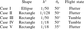
List of simulation cases with different shapes and
 $\unicode[STIX]{x1D703}_{0}$
at
 $Re=80$
and
 $I^{\ast }=3.0$
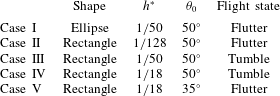
, corresponding to those in figure 19.
The investigation of bistability is extended to rectangular and elliptic plates of different thicknesses. Note that an elliptical plate of the same thickness has a lower moment of inertia than a rectangular plate, expressed as
 ${I^{\ast }}_{ellipse}=\unicode[STIX]{x1D70C}^{\ast }h^{\ast }(1+h^{\ast })/2$
. Table 4 lists five cases of different shapes and
 $\unicode[STIX]{x1D703}_{0}$
at
 $Re=80$
and
 $I^{\ast }=3.0$
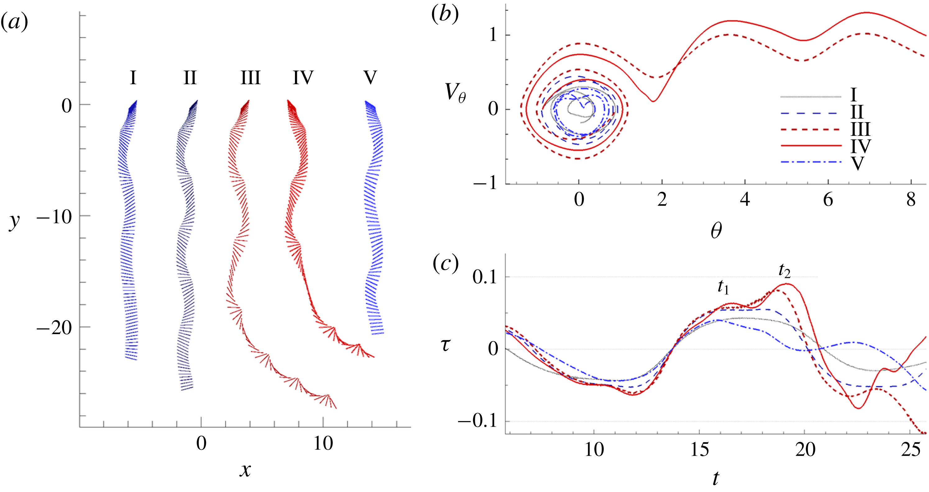
, with results presented in figure 19. Consider case II of
 $h^{\ast }=1/128$
and case III of
 $h^{\ast }=1/50$
, they respectively develop into stable falling and tumbling as per figure 19(a). It can be seen that case III climbs towards a second
 $\unicode[STIX]{x1D70F}_{max}$
at
 $t_{2}$
in figure 19(c), and thus reaches sufficient
 $V_{\unicode[STIX]{x1D703}}$
towards tumbling motion, while case II converges to the fixed point from the phase portraits in figure 19(b). In fact, comparing cases II–IV of increasing
 $h^{\ast }$
reveals that
 $\unicode[STIX]{x1D70F}$
at
 $t_{2}$
is progressively increased in figure 19(c). Case IV exhibits larger degrees of rotation
 $\unicode[STIX]{x1D703}$
(the cause of which is given in the discussion of figure 21), arriving quickly at the saddle point at
 $\unicode[STIX]{x03C0}/2$
shown in figure 19(b), causing the plate to tumble sooner than case III. Considering again case III, now compared against case I that is elliptically shaped. Figure 19(c) shows that case I is decreasing at
 $t_{2}$
and does not climb to a second
 $\unicode[STIX]{x1D70F}_{max}$
, but has its motion decaying rapidly into stable falling. This shows that the tendency for a rectangular plate to tumble is higher. Lastly, as the initial angle of release is reduced from case IV at
 $\unicode[STIX]{x1D703}_{0}=50^{\circ }$
to case V at
 $\unicode[STIX]{x1D703}_{0}=35^{\circ }$
, the same plate settles into stable falling through diminishing its motion into the fixed point (0,0) as seen in figure 19(b), portraying the bistable behaviour at a higher
 $h^{\ast }$
. The general effect of
 $h^{\ast }$
on the bistability is outlined in the following discussion.
(a) Relationship between the critical initial angle
 $\unicode[STIX]{x1D703}_{0cr}$
(deg) and
 $I^{\ast }$
at
 $Re=80$
for the nominal plate and the rectangular plate of
 $h^{\ast }=1/18$
; (b) variations of
 $\unicode[STIX]{x1D703}_{0cr}$
for different geometries at
 $Re=80$
and
 $I^{\ast }=3.0$
. Note that rectangle of
 $h^{\ast }=1/4$
does not progress into tumble at any
 $\unicode[STIX]{x1D703}_{0}$
.

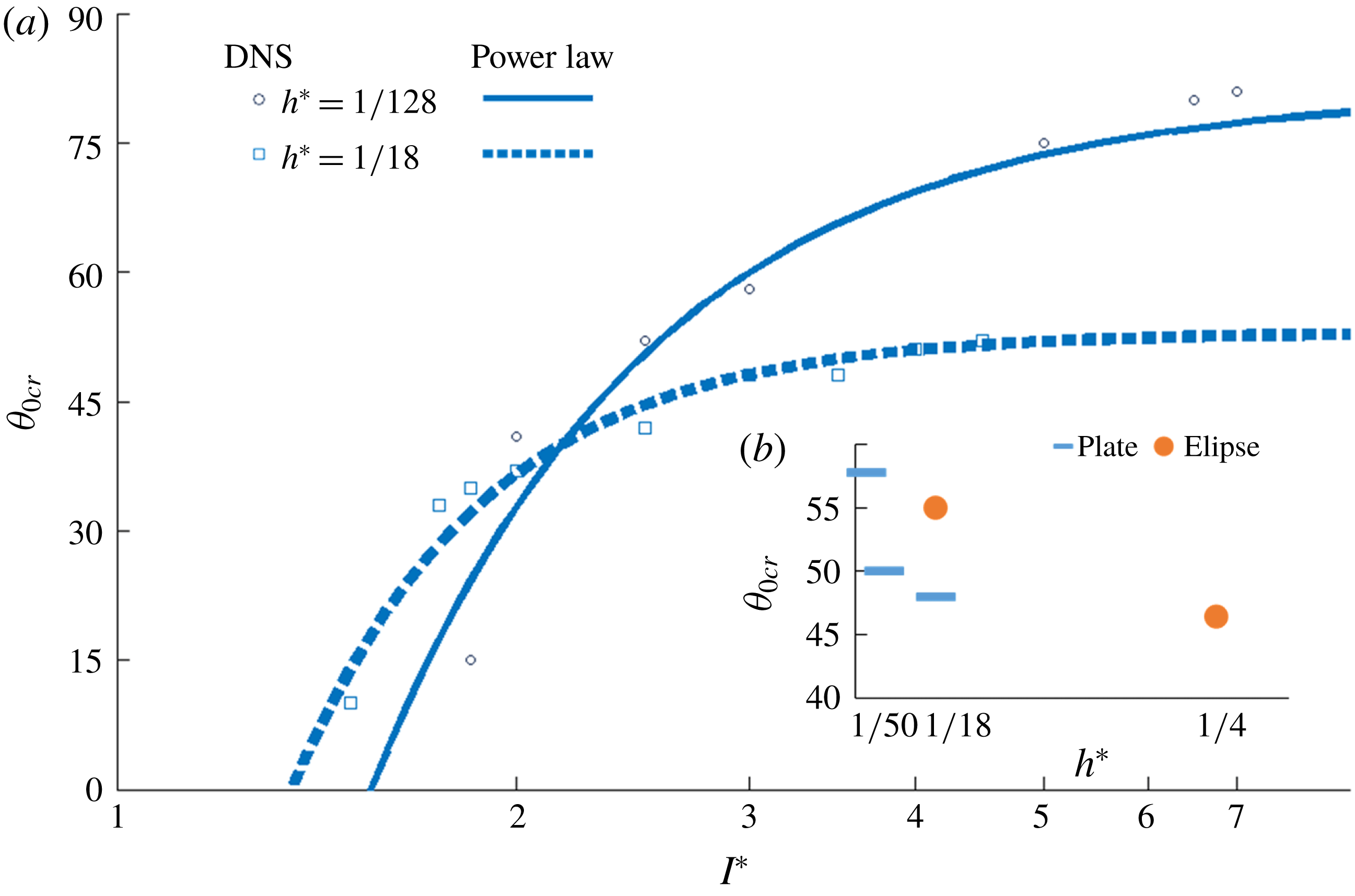
The variation of
 $\unicode[STIX]{x1D703}_{0cr}$
that separates the two bistable states for
 $h^{\ast }=1/18$
is produced in figure 20(a). The downward shift of the
 $\unicode[STIX]{x1D703}_{0cr}$
relationship for
 $h^{\ast }=1/18$
indicates its higher tendency to tumble when compared to the nominal plate of
 $h^{\ast }=1/128$
.
 $\unicode[STIX]{x1D703}_{0}$
. In turn, it also suggests that the bistable mapping provided in figure 9 would generally shift upwards for thicker plates with the same
 $I^{\ast }$
. The
 $\unicode[STIX]{x1D703}_{0cr}$
becomes more invariant with
 $Re$
, an observation also observed by Mittal et al. (Reference Mittal, Seshadri and Udaykumar2004). Figure 20(b) further highlights the changes of
 $\unicode[STIX]{x1D703}_{0cr}$
, for rectangular plates compared with elliptical ones. The higher tendency for rectangles to tumble is related to the flow fields affected by the differences in cross-sectional area and the smoothness of the edges.
Snapshots of stable falling plates of
 $Re=80$
,
 $I^{\ast }=3.0$
, with
 $\unicode[STIX]{x1D703}_{0}=45^{\circ }$
at the same turning point for rectangles of (a,e)
 $h^{\ast }=1/18$
and (b,f)
 $h^{\ast }=1/4$
, and ellipses of (c,g)
 $h^{\ast }=1/18$
and (d,h)
 $h^{\ast }=1/4$
. The falling plates are turning clockwise. Vorticity and velocity fields are on the top row. Pressure fields are on the bottom row.

The flow fields in figure 21 compare the flow fields of different shapes for bistability behaviour. From figure 21(a,b), the leading edge vortex and pressure gradient are stronger for thicker plates. The same observation is found on comparing elliptical plates in figure 21(c,d). The increase in
 $h^{\ast }$
results in more compact and intense flow structures as the cross-sectional areas are substantially increased, displacing more flow. Comparing now the rectangular and elliptical plates, figure 21(b), with larger cross-sections, these also display larger displacements of both the flow and the dynamics for the vortices to engulf the upper surface. Owing to the sharp geometry and the increased form drag, the leading edge vortex is shed upwards and also to right along the surface in these cases; and the trailing edge vortex is shed away from the corner of the lower surface. This leads to a more volatile oscillation for rectangular plates than for their elliptical counterparts in figure 21(d).
Indeed, bistability arises for other geometries and thicknesses. The increased intensity of vortical structures produce more torque, e.g. in figure 19(c), in favour of tumbling at lower critical angles
 $\unicode[STIX]{x1D703}_{0cr}$
for higher
 $h^{\ast }$
and for rectangular plates in figure 20. However, if
 $h^{\ast }$
is too large, e.g. at
 $h^{\ast }=1/4$
, there is no development of tumbling anymore, despite the volatile movement. This is in agreement with Mittal et al. (Reference Mittal, Seshadri and Udaykumar2004). The effect of the shape can be further studied through conducting the mapping through a range
 $h^{\ast }$
for heavy plates, similar to the work of Zhou, Chrust & Dušek (Reference Zhou, Chrust and Dušek2017) on three-dimensional oblate spheroids.
4 Conclusion
The free falling of heavy plates has been numerically investigated by using the immersed boundary method. Beginning from a discussion on stable fall, the analysis of the simulations reveals how heavy plates evolve into tumbling. Through the transition, it is found that both stable falling and tumbling are possible, subject to the initial angle
 $\unicode[STIX]{x1D703}_{0}$
. This new observation is different from other flight states that were originally suggested to be invariant on the initial angle (Andersen et al.
Reference Andersen, Pesavento and Wang2005b
; Wan et al.
Reference Wan, Dong and Liang2012; Wu & Lin Reference Wu and Lin2015). The bistable behaviour fulfils the mapping of heavy plates, resolving the regime previously mixed with erratic oscillating fall and tumble. A power law is produced describing
 $\unicode[STIX]{x1D703}_{0cr}$
, the critical initial angle separating the bistable flight states, in relation to
 $Re$
and
 $I^{\ast }$
for a specified
 $h^{\ast }$
. Detailed analysis of flow fields reveals that the onset of the two states are related to the lift curve. Plates developing towards tumbling are also characterised by the additional generation of torque from the recirculation behind the plate; and that
 $\unicode[STIX]{x1D703}_{0}$
governs the field of this recirculation. The flight mechanics and bistable behaviour are also depicted in the experiment conducted. Together with DNS results for different shapes, the effect of the downstream vortex system on bistability is further discussed. While a vast number of studies providing the relationships between wake formations and flight states, this study further abridges the two by resolving the cause-and-effect within the FSI of the free falling problem. The insight into the flight progression of heavy plates, and its bistability characteristics could lead to further understanding of natural phenomena and could potentially be applied to passive flight control.
Acknowledgements
This work was supported by the National Natural Science Foundation of China (grant numbers 11772172 and 11490551). We thank Dr Y. X. Jia and Kenneth M. Lau for their technical support in carrying out the experiments. We also like to thank Professor Daniel Weihs for the inspiring discussion.