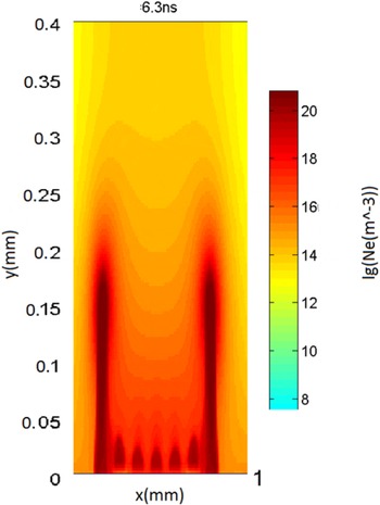
1. Introduction
Developed leaders (Bazelyan & Raizer Reference Bazelyan and Raizer1998) represent highly conductive plasma channels, continuously emitting a fan of streamers, termed the streamer zone. The leader tip moves at a speed much slower than that of individual streamers. Gas in the leader channel is heated by the current. A huge number of short-lived streamers in the corona generate the space charge field required to maintain the streamers propagation. As streamers move along some distance until termination, their charge covers the leader channel and prevents its expansion and cooling.
Gallimberti (Reference Gallimberti1979) and Gallimberti et al. (Reference Gallimberti, Bacchiega, Bondiou-Clergerie and Lalande2002) first noted that the development of atmospheric lightning is initiated and sustained by the formation of streamer corona and leader discharges in air, very similar to those observed in laboratory long sparks. A number of different models of the lightning leader have since been proposed. Arevalo et al. (Reference Arevalo, Cooray, Wu and Jacobson2012) used a simplified electrostatic approximation to describe the streamer zone for long spark gaps. Naidis (Reference Naidis2009) studied positive and negative streamers in air.
Bazelyan, Raizer & Aleksandrov (Reference Bazelyan, Raizer and Aleksandrov2007) and Popov (Reference Popov2009) presented a 1-D model of leader formation and propagation. In this model the formation of a leader is governed by the contraction of the current of a streamer flash into a small radius channel, and ultimately by its heating of the gas to the temperature characteristic of an arc discharge. Shneider, Mokrov & Milikh (Reference Shneider, Mokrov and Milikh2012, Reference Shneider, Mokrov and Milikh2014) were first to introduce 2-D simulations of the dynamic contraction in a self-sustained glow discharge. da Silva & Pasko (Reference da Silva and Pasko2013) discussed a 1-D model of streamer-to-leader transition, while Bonaventura et al. (Reference Bonaventura, Bourdon, Celestin and Pasko2011) discussed the current status of simulations of streamer discharges in air.
Interactions of streamers in air has been the subject of number of studies. Naidis (Reference Naidis1996) studied the corrections to the streamer velocity due to electrostatic interaction with neighbouring streamers using a quasi-2-D positive streamer model. Bonaventura et al. (Reference Bonaventura, Duarte, Bourdon and Massot2012) simulated the interaction of two streamers which are attracted due to photoionization and will eventually merge. Luque, Ebert & Hundsdorfer (Reference Luque, Ebert and Hundsdorfer2008) simulated the interaction of two 3-D streamers and studied the effects of electrostatic repulsion and attraction due to non-local photoionization. Babaeva & Kushner (Reference Babaeva and Kushner2014) used a 2-D model to simulate the interaction of one-, two- and three-plasma jet arrays. Despite significant progress, the critical issue of the model, which is the conversion from the streamer to the leader phase, remains unresolved.
The objective of this paper is to present 2-D plasma simulations of the formation and propagation of the streamer zone of a leader. In these simulations we generate a group of streamers that propagate in a discharge gap while interacting with each other. It is shown that interactions between the streamers significantly reduce their propagation velocity. This explains why the leader, which consists of many streamers, is much slower than a single streamer formed in the same discharge gap.
2. Computational model
We use the modified numerical model (Likhanskii et al.
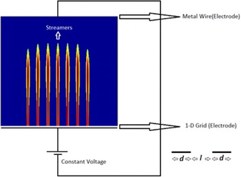
Reference Likhanskii, Shneider, Macheret and Miles2007, Reference Likhanskii, Shneider, Macheret and Miles2008) developed to simulate discharge plasma actuators driven by nanosecond pulses. The model, a schematic of which is shown in figure 1, uses a 2-D rectangular computational box. Two electrodes are located at the top and bottom of the box. The bottom electrode is made of a 1-D grid with each of its nodes having size
 $d$
, and the distance between two adjacent nodes is
 $l$
. Such a configuration allows for the generation of a group of interacting streamers. A constant voltage is applied to the electrodes. The discharge gap is filled with the air at normal conditions.
Schematic of the simulation model. 2-D rectangular computational box is filled with the air at normal conditions. The constant voltage is applied to the electrodes, of which the bottom electrode is a 1-D grid. It consists of nodes having size
 $d$
while the distance between two adjacent nodes is
 $l$
(see the sketch at the bottom right-hand corner). The streamers start from the conducting nodes.

The model considers electrons, positive and negative ions. The formation of negative ions is due to the attachment of electrons to molecular oxygen. The plasma kinetics and interactions with neutral molecules are modelled using a drift-diffusion approximation (Boeuf & Pitchford Reference Boeuf and Pitchford2005; Likhanskii et al.
Reference Likhanskii, Shneider, Macheret and Miles2007). The continuity equations for electrons and positive and negative ions are solved numerically using the set of the proper reaction rates taken from Likhanskii et al. (Reference Likhanskii, Shneider, Macheret and Miles2008). Ionization and recombination coefficients, as well as attachment, detachment rates, charged particles mobility and electron temperature are considered to be functions of the reduced electric field
 $E/N$
(
 $N$
is the air number density). The electric field and potential are related to the density of charged species according to the Poisson equation.
In this paper we focus on positive leaders which propagate in pre-existing weakly ionized plasma. Thus we consider the anode located on the bottom of the discharge gap. As the initial condition we chose the uniform quasi-neutral plasma density, equal to
 $n_{0}=10^{10}~\text{m}^{-3}$
. This provides sufficiently fast ionization during the early stage of the discharge. We use
 $d=0.03~\text{mm}$
as the initial condition.
We used Neumann boundary conditions on the lateral sides of the computational domain, and Dirichlet boundary conditions (electric field perpendicular to the surface) on the top boundary. The applied voltage produced a weakly ionized plasma near the edge of the bottom electrode (anode), which subsequently spread towards the cathode. The boundary condition at the anode surface is given by the upward moving electron flux due to secondary emission with emission coefficient 0.1 (Likhanskii et al.
Reference Likhanskii, Shneider, Macheret and Miles2007). We chose an applied potential of 3.5 kV which corresponds to the reduced electric field
 $E/N=280$
Td. (Townsend is a physical unit of the reduced electric field
 $E/N$
,
 $1~\text{Td}=10^{-21}~\text{V}~\text{m}^{2}$
. It is used in gas discharge physics, where
 $E/N$
serves as scaling parameter because the mean electron energy is a function of
 $E/N$
.) It is approximately 2.5 times higher than the breakdown field, thus the streamers develop inside the discharge gap within a few ns. To model plasma kinetics we used the Euler scheme for the continuity equations with a Scharfetter–Gummel scheme for charged species fluxes.
To solve the Poisson equation we used the successive over-relaxation method. The time step was chosen in such a way that it allows resolution of the plasma formation which is of the order of nanoseconds. In addition, the time step should satisfy the Courant–Friedrichs–Lewy (CFL) condition. The combination of these two requirements leads to the time step of the order of picoseconds (Likhanskii et al. Reference Likhanskii, Shneider, Macheret and Miles2007).
The chosen size of the computational box is broad enough to allow the multiple streamers to avoid effects from the
 $y$
-boundaries. The box is also tall enough that the streamers become well developed before they reach the upper boundary. The computations were conducted at the University of Maryland Cluster where 40 processors were used for a run.
In this paper we ignore the effect of photoionization since our focus is on positive streamers. Future work will present simulations of negative streamers also, where photoionization will be considered.
3. Results of simulations
First we study the formation and propagation of a single streamer. We will describe the temporal evolution of the electron density as well as the electric fields. Then we will discuss the formation and propagation of a simultaneously incepted group of streamers and compare the data with those related to the single streamer. Finally, we consider the formation of two groups of streamers, one incepted with some delay with respect to the other group, and compare them with the single streamer.
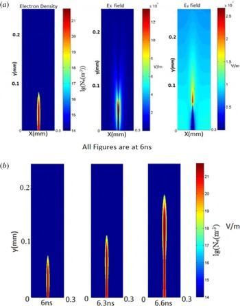
(a) The plasma density and
 $x$
- and
 $y$
-components of the electric field at the elapsed time
 $t=6~\text{ns}$
. (b) The streamers are shown at the different elapsed times.

3.1. Single streamer
Figure 2(a) shows the spatial distribution of the plasma density and
 $x$
- and
 $y$
-components of the electric field after
 $t=6~\text{ns}$
. The colour maps show the logarithm of the electron density given in
 $1~\text{m}^{-3}$
and the electric field in
 $\text{V}~\text{m}^{-1}$
. The far left-hand panel shows the streamer having a needle like shape, with its tip at
 $y_{tip}=0.8\times 10^{-4}~\text{m}$
. The colour maps show the lg scale of the electron density. The strongest electron density occurs in the streamer’s body at
 $y<0.64\times 10^{-4}~\text{m}$
. The vertical component of the electric field
 $E_{y}$
exceeds the breakdown threshold of the air (
 $3~\text{MV}~\text{m}^{-1}$
) in the vicinity of the streamer tip. Thus the
 $E_{y}$
field component plays the main role in the streamer formation, while the
 $E_{x}$
component is of much smaller amplitude. Thus the
 $E_{x}$
field will be ignored in the following analysis.
Note that the mean streamer velocity at a given time
 $t$
is determined by its length, which in turn depends on the location of the tip
 $V_{o}=y_{tip}(t)/t$
.
Figure 2(b) shows the streamer growth versus the time elapsed. It is apparent that the streamer length nonlinearly depends on the time, namely the closer the streamer tip to the top electrode, the higher is the velocity. Further, as the time reaches approximately 6.7 ns, the streamer touches the electrode, thus ending the simulations.
3.2. Simultaneously incepted multiple streamers
Now we simulate the formation and propagation of a group of simultaneously incepted streamers separated by a distance of
 $l$
. The main parameter of the problem is the ratio
 $l/d$
which determines the interaction between the streamers. Here,
 $d$
is the horizontal size of the streamer base (i.e. the size of the conducting node). In these simulations we use
 $d=3\times 10^{-5}~\text{m}$
,
 $l$
varies in the range
 $3\times 10^{-5}$
to
 $2.1\times 10^{-4}~\text{m}$
and the horizontal scale of the computational domain is
 $4\times 10^{-3}~\text{m}$
.
We chose seven streamers for our simulations for the following reasons: (i) it is a sufficient number of streamers to demonstrate the ‘collective effect’ when the interaction is determined not only by the close neighbours, but the distant streamers as well, and (ii) we will vary the inter-streamer distance, or
 $l/d$
ratio, which increases the size of the computational box. The latter is controlled by the limited computational resources.
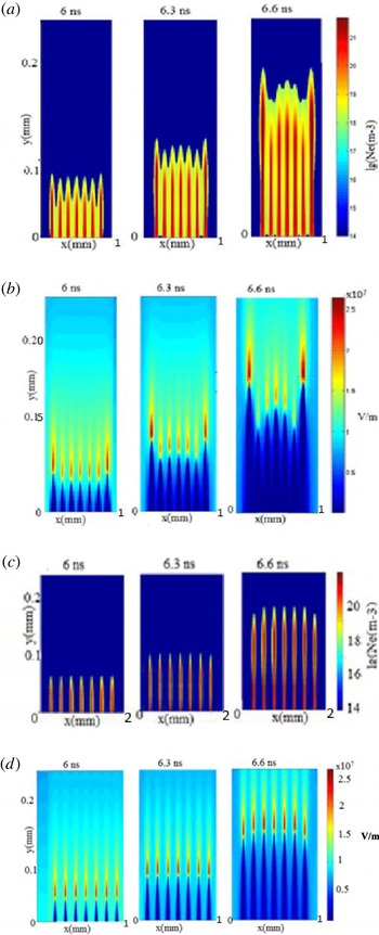
Formation and propagation of 7 interacting streamers; (a) simulations for
 $l/d=2$
, three plasma density images correspond to elapsed times of
 $=$
6.0, 6.3 and 6.6 ns; (b) the related
 $E_{y}$
fields at 6.0, 6.3 and 6.6 ns; (c) plasma density for
 $l/d=6$
at the three elapsed times 6.0, 6.3 and 6.6 ns; (d) the related
 $E_{y}$
fields.

An example of such modelling is shown in figure 3 where 7 streamers, separated by a varying distance (
 $l/d=2$
and 6), were simulated. Three images in figure 3(a) show the plasma density obtained at 6.0, 6.3 and 6.6 ns. Figure 3(b) reveals the related
 $E_{y}$
field found at the same times. Figure 3(a,b) shows the dynamics of the streamers formation. Namely, at
 $t=6.0~\text{ns}$
, all seven streamers are of approximately the same length and electron density, and the
 $E_{y}$
field is approximately the same for all streamers, except for some amplitude magnification at the edges. When the elapsed time increases, the two outermost streamers grow faster and the ionizing
 $E_{y}$
field is stronger than for the other five streamers. The streamers suppression is due to the electrostatic repulsion which depends on the distance between the streamers tips. In fact, the two outermost streamers experience a strong interaction only with one close neighbour, while the rest of the streamers mostly interact with the two closest neighbours, one at each side. Thus streamers 2–6 are strongly suppressed by the powerful outermost neighbours.
Moreover, it is apparent from comparison of figures 2 and 3 that the interactions between the streamers suppress their length
 $y_{tip}(t)$
, and thus reduce their mean velocity
 $V=y_{tip}/t$
. We will discuss this effect in detail in the Discussion section. When the
 $l/d$
ratio reached 6 (see figure 3
c,d) the outermost streamers look the same as the other, i.e. no interaction between the streamers occurs.
In Appendix we have added three figures showing the plasma density for a group of close streamers (
 $l/d=1$
), and the vertical component of the electric field for
 $l/d=2$
and 6.
3.3. Multiple streamers incepted with some delay with respect to each other
Generally speaking, the streamers in the streamer zone of a leader can be incepted at different times. Therefore we will analyse how the delay in the injection of different streamers affects the mean propagation velocity of the streamer zone.
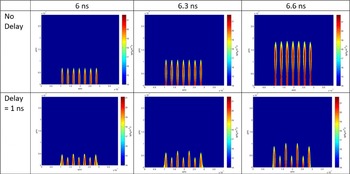
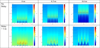
Plasma density computed for
 $l/d=5$
; (the top row) simultaneously incepted streamers depicted at 6.0, 6.3 and 6.6 ns; (the bottom row) the same conditions as above except that the odd streamers are delayed by 1 ns with respect to the even streamers.

The top panels in figure 4 show the group of simultaneously incepted seven streamers depicted at 6.0, 6.3 and 6.6 ns. We chose a
 $l/d$
ratio equal to 5 in order to avoid the streamers interacting, as is apparent from the top images. The bottom panels show simulations made under the same conditions as above, except that the even streamers are incepted at
 $t=0$
while the odd streamers are delayed by 1 ns. A comparison between the top and bottom panels shows that the even streamers are suppressed and are moving much slower than those incepted simultaneously.
Thus the 1 ns delay increases the interaction between the streamers, which leads to the suppression of their average velocity.
Figure 5 shows the vertical component of the electric field simulated for the same conditions as in figure 4. In fact, the bottom panel simulated at 1 ns delay between the even and odd streamers shows that a strong electric field
 $E_{y}$
evolves in the tips of streamers 3 and 5.
4. Discussion
In this section we will discuss how the interactions between the streamers affects the formation and propagation of the streamer zone of a leader. We consider first a group of simultaneously incepted streamers.
The vertical component of the electric field simulated for the same conditions as in figure 4.

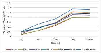
Mean streamer velocity versus the elapsed time computed for different inter-streamer distances (
 $l/d=2,3,\ldots ,7$
) along with the velocity of the single streamer.

Figure 6 shows the mean streamer velocity versus the elapsed time computed for different inter-streamer distances (
 $l/d=2,3,\ldots ,7$
). The figure includes also the time-dependent velocity of the single streamer. Since the streamer images were not detected before 5 ns, the space between 0 and 5 ns is blank. As shown earlier in figure 2(b), the mean velocity of the single streamer slowly increases with time between 6.0 and 6.3 ns, then from 6.3 to 6.6 ns the streamers grow faster. Finally the velocity reaches saturation at
 $t>6.6~\text{ns}$
when the streamers touch the top electrode. It should be noted that the velocity is suppressed at the close inter-streamer distance (
 $l/d<5$
) due to interactions between the streamers. At a longer inter-streamer distance (
 $l/d>6$
), the streamers behave as though they are not interacting.
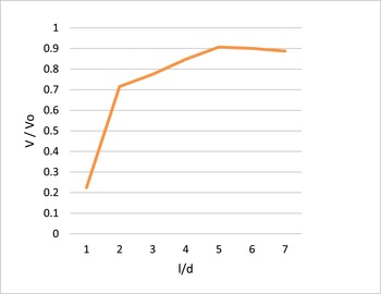
The mean streamer velocity normalized by that of the single streamer (
 $V/V_{o}$
) versus
 $l/d$
ratio obtained at 6.3 ns.

Figure 7 reveals how the variation of the distance between the streamers affects their mean propagation velocity. It shows the ratio
 $V/V_{o}$
i.e. the mean velocity normalized by that of the single streamer, versus the
 $l/d$
ratio obtained at 6.3 ns. The figure reveals that at close inter-streamer distances
 $l/d=1{-}2$
, the streamer interactions and thus the velocity suppression are very strong
 $(V/V_{o}<0.7)$
, at
 $2<l/d<5$
it is intermediate
 $(V/V_{o}<0.9)$
, and at higher
 $l/d>5$
the
 $V/V_{o}$
ratio tends to unity. At such an inter-streamer distance, the streamers stop interacting, thus they behave like a single streamer incepted in the discharge gate.
Moreover, at the given electric field, we can find a value of the
 $l/d$
ratio
 $(l/d=5)$
at which the suppression of the streamer velocity becomes noticeable (reaches 20 %).
We now discuss this phenomenon in terms of packing factor (Pac), which is the fraction of the volume of a discharge gap that is occupied by the streamers. In the case of a 2-D model, the volume will be substituted by the area filled with the simultaneously incepted streamers all having the length
 $y_{str}$
, here the Pac yields:
 $$\begin{eqnarray}\text{Pac}=\frac{d\times y_{str}}{l\times y_{str}+d\times y_{str}}=\frac{1}{1+l/d}.\end{eqnarray}$$
Thus the Pac is determined by the
 $l/d$
ratio only. As was shown above at
 $l/d>4$
, the interactions between streamers can be neglected. This gives us the critical value of
 $\text{Pac}=0.2$
which describes a transition between interacting and non-interacting streamers.
Notice that the major goal of this work is not the development of an advanced model of streamers, but an attempt to understand the packing factor in the streamer corona. Therefore the focus is on studying an ensemble of 7 streamers. Considering the existing computational resources, it is not feasible to run 3-D numerical models to describe multiple streamers. We thus use a simplified 2-D model. We expect that the major physics will not change when switching from a 2-D to 3-D model, although some coefficients will be affected.
Let us consider how the delay of a subgroup of the streamers affects the mean propagation velocity.
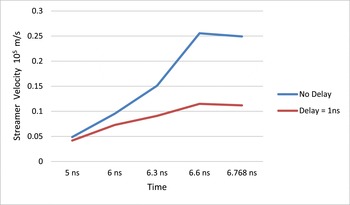
The temporal variations of the mean propagation velocity
 $V$
of the streamers all simultaneously incepted at
 $t=0$
(the blue curve) and that where the odd streamers are delayed by 1 ns (the red curve). They are computed for
 $l/d=5$
.

Figure 8 shows the temporal variations of the mean propagation velocity of the streamers simultaneously incepted at
 $t=0$
(the blue curve) and that where the odd streamers are delayed by 1 ns (the red curve). In the latter case, the mean velocity was found by averaging the seven streamers velocities.
5. Conclusions
We have presented a model for the formation and propagation of the streamer zone of a leader which is an outstanding problem in the physics of electric discharges. The model is based on 2-D plasma simulations which use the modified code originally developed by Likhanskii et al. (Reference Likhanskii, Shneider, Macheret and Miles2007, Reference Likhanskii, Shneider, Macheret and Miles2008). As a first step we have developed a model that simulates formation and propagation of a single positive streamer in a pre-existing weakly ionized plasma in a discharge gap filled with air at normal conditions. Then, the model was generalized to describe the formation of multiple interacting positive streamers injected in the discharge gap, either simultaneously or with some delay with respect to each other.
We found that the mean velocity of the group of simultaneously injected streamers is less than that of a single streamer. This is the first time the velocity suppression due to interactions between the streamers has been simulated. It could explain why the streamer zone of a leader is much slower than a single streamer formed in the same discharge gap.
Finally, it has been shown that the velocity suppression is determined by the inter-streamer distance, or more precisely by the
 $l/d$
ratio, where
 $l$
is the distance between two adjacent grid nodes and
 $d$
is the size of a grid node. We found the critical value of the
 $l/d$
ratio of the streamers at which the interactions between the streamers can be neglected, and thus the process can be treated as caused by a group of non-interacting streamers. The critical value of the
 $l/d$
ratio was presented in terms of the streamer packing factor. Moreover, it was shown that the delay between two groups of the streamers intensifies their interactions and thus further reduces their mean propagation velocity. The results of the presented model are relevant to the study of laboratory leaders and leaders formed by lightning.
Acknowledgements
This work was supported by NSF grant 1226237. The authors acknowledge University of Maryland super computer resources (http://www.it.umd.edu/hpcc) made available for conducting the research reported in this paper.
Appendix
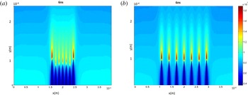
The Appendix contains some additional images of the multiple streamers along with comments.
Plasma density for the set of 7 strongly interacting streamers,
 $l/d=1$
, computed for the elapsed time
 $t=6.3~\text{ns}$
.

Figure 9 shows plasma density for the set of 7 very close streamers,
 $l/d=1$
. The elapsed time
 $t=6.3~\text{ns}$
. The figure reveals that the amplitudes of the inner 5 streamers, 2–6, are strongly reduced due to the inter-streamer interactions. The amplitudes of two streamers at the edges, 1 and 7, are much higher than those of the inner streamers. A comparison with the middle panel of figure 3(a) computed at
 $l/d=2$
shows that streamer interactions increase drastically when the inter-streamer distance is compressed from
 $l=2d$
to
 $l=d$
.
The vertical component of the electric field for
 $l/d=2$
(a) and
 $l/d=6$
(b) computed for the elapsed time
 $t=6~\text{ns}$
.

Figure 10 shows the vertical component of the electric field for two values of the
 $l/d$
ratio,
 $l/d=2$
(a) and
 $l/d=6$
(b). The elapsed time
 $t=6~\text{ns}$
. (a) Reveals that at the close distance between the streamers with
 $l/d=2$
, the field of the inner five streamers, 2–6, is reduced due to the streamer interactions. The field caused by the two streamers at the edges, 1 and 7, is much stronger.
Figure 10(b) shows that the electric field of the streamers located at a distance
 $l/d=6$
are the same for any of the streamers. This implies that the streamers interact only weakly.