1. Introduction
Wall shear stress (WSS) is the tangential component of traction on the wall. WSS provides two types of information. First, it can be used to quantify the frictional drag force per unit area on the wall. Second, it provides a first-order approximation for near-wall convective transport. In the context of mass or heat transfer, the importance of near-wall flow is emphasized in high-Schmidt-number (
 $Sc$
) or high-Prandtl-number (
 $Pr$
) open flows with a flux of species concentration or heat at the wall, and a convection-dominated free stream carrying a specific species concentration or temperature over the no-slip boundary. In this paper, we focus on high-
 $Sc$
mass transfer; however, the ideas could be used in high-
 $Pr$
heat transfer applications as well.
Mass transfer in the cardiovascular system, including the transport of solutes (e.g. oxygen and nutrients) or that of proteins and cells (e.g. low-density lipids and blood cells), represents an important application of high-
 $Sc$
flows (Ethier Reference Ethier2002). The methods presented herein will be applied to pulsatile blood flow inside an abdominal aortic aneurysm (AAA). AAA is a permanent widening of the aorta in the abdominal region. The sudden expansion of the aorta, complex vascular anatomy, the presence of branch arteries and pulsatility of blood flow together lead to complex flow inside AAAs (Finol & Amon Reference Finol and Amon2001; Deplano et al.
Reference Deplano, Knapp, Bertrand and Gaillard2007; Arzani & Shadden Reference Arzani and Shadden2012), accompanied by complex WSS distributions (Salsac et al.
Reference Salsac, Sparks, Chomaz and Lasheras2006) and particle residence times (Suh et al.
Reference Suh, Les, Tenforde, Shadden, Spilker, Yeung, Cheng, Herfkens, Dalman and Taylor2011a
,Reference Suh, Tenforde, Shadden, Spilker, Cheng, Herfkens, Dalman and Taylor
b
).
It is known that, in convection-dominated flows, a flux of species concentration at the wall will lead to the formation of a thin concentration boundary layer. The common approach to obtain the species concentration distribution is to solve the advection–diffusion equation in an Eulerian framework. However, this approach requires an extremely high resolution near the wall, often leading to numerical difficulties in complex three-dimensional (3D) flows (Ethier Reference Ethier2002). Alternatively, in the case of high-
 $Sc$
flows, the near-wall region can be considered isolated from the rest of the flow, with the core flow having negligible direct effect on the concentration distribution. Because the WSS vector field can be scaled to obtain a first-order approximation for the velocity vector field next to the wall, it may be used to compute surface-bound trajectories representing the transport of a material species near the wall. In the case of high
 $Sc$
, the concentration boundary layer is very thin, making this first-order approximation reasonable for understanding near-wall transport.
Previous studies have shown that, for a prescribed concentration (Dirichlet boundary condition) on the wall, the resulting flux of concentration from the wall is mostly independent of the chaotic flow away from the wall (Ghosh, Leonard & Wiggins Reference Ghosh, Leonard and Wiggins1998). The observation that the boundary layer distribution of a concentration is largely unaffected by advection far from the wall motivates a reduced-order near-wall approach, which can be based on the WSS vector field. It should be noted, however, that the large-scale core flow features determine the WSS patterns (El Hassan et al. Reference El Hassan, Assoum, Martinuzzi, Sobolik, Abed-Meraim and Sakout2013), and therefore the near-wall transport depends on the flow topology away from the wall indirectly.
In prior work, critical points of the WSS vector field and their dynamics have been observed to play an important role in organizing near-wall transport (Perry & Chong Reference Perry and Chong1987; Cardesa et al. Reference Cardesa, Monty, Soria and Chong2014). Also, the structure of WSS lines have been used in developing theories for flow separation using dynamical system methods (Surana, Grunberg & Haller Reference Surana, Grunberg and Haller2006; Surana et al. Reference Surana, Jacobs, Grunberg and Haller2008). Recently, WSS critical points associated with rare near-wall backflow have been observed in turbulent channel flows (Lenaers et al. Reference Lenaers, Li, Brethouwer, Schlatter and Örlü2012; Brücker Reference Brücker2015). WSS patterns have been demonstrated to affect the heat transfer in impinging jets. As examples, the heat transfer coefficient has been shown to have a similar distribution as WSS with a phase shift (Hadžiabdić & Hanjalić Reference Hadžiabdić and Hanjalić2008), and Dairay et al. (Reference Dairay, Fortuné, Lamballais and Brizzi2015) showed that the secondary vortex resulting from flow impingement creates negative WSS regions that correspond to heat transfer augmentation.
The correlations observed in the above studies between WSS and transport processes motivates a more mechanistic exploration of near-wall flow topology induced by the WSS vector field. In steady flows the critical points of the vector field and their associated invariant manifolds largely determine the flow topology. In unsteady flows Lagrangian coherent structures (LCS) have been used to obtain a template for transport (Shadden Reference Shadden2011; Haller Reference Haller2015), including cardiovascular applications (Shadden & Taylor Reference Shadden and Taylor2008; Shadden & Arzani Reference Shadden and Arzani2015). These structures represent prominent flow features that organize the flow from a Lagrangian perspective. This study demonstrates the relevance of similar structures obtained from the WSS vector field for organizing near-wall transport in the context of patient-specific AAA models. Namely, species accumulation in the boundary layer in connection with these structures will be demonstrated. The influence of diffusion and flow normal to the wall is also investigated and discussed.
2. Methods
Velocity data were obtained from computational fluid dynamics (CFD) simulations of blood flow in two patient-specific AAA models, as described in Arzani et al. (Reference Arzani, Suh, Dalman and Shadden2014b
). The vascular models spanned from the descending aorta through the iliac arteries to ensure the region of interest (aneurysm) was sufficiently far from inflow and outflow boundaries. Major aortic branch arteries were also included due to their proximal influence on abdominal aortic flow. Inflow and outflow boundary conditions were tuned to match measured patient-specific flow rates and blood pressures as described in Les et al. (Reference Les, Shadden, Figueroa, Park, Tedesco, Herfkens, Dalman and Taylor2010). Rigid wall and Newtonian blood rheology were assumed. It has been shown that the Newtonian assumption produces reasonable WSS patterns in AAAs (Marrero et al.
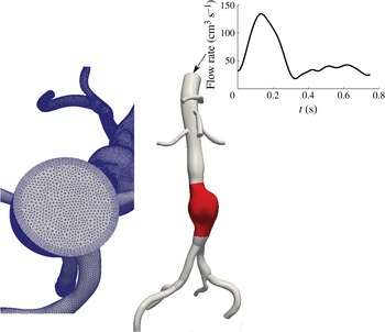
Reference Marrero, Tichy, Sahni and Jansen2014) and that vessel deformation leads to relatively minor changes in overall flow topology (Duvernois, Marsden & Shadden Reference Duvernois, Marsden and Shadden2013). Figure 1 shows one of the two AAA models, to exemplify the anatomy of the model, the morphology of the volumetric flow waveform and the nature of the mesh. The results presented in this paper are mostly based on this model for demonstration purposes, although similar results were observed for other patient-specific geometries. The incompressible Navier–Stokes equations were solved using the stabilized finite element flow solver in SimVascular (http://simvascular.github.io/). Linear tetrahedral elements, with second-order time integration were used. The mesh edge size next to the wall was
 $200~{\rm\mu}\text{m}$
, and the time step divided the cardiac cycle into 1000 time points. The peak Reynolds number was
 $Re=1750$
and the Womersley number was
 ${\it\alpha}=12.8$
. The wall traction was obtained as
 $\boldsymbol{t}={\bf\sigma}\boldsymbol{\cdot }\boldsymbol{e}_{n}$
, with the stress tensor
 ${\bf\sigma}$
and the unit normal vector
 $\boldsymbol{e}_{n}$
evaluated on the wall. The WSS vector was computed as
 $$\begin{eqnarray}{\bf\tau}=\boldsymbol{t}-(\boldsymbol{t}\boldsymbol{\cdot }\boldsymbol{e}_{n})\boldsymbol{e}_{n}.\end{eqnarray}$$
The convective near-wall transport can be derived by Taylor expansion of the fluid velocity near the wall (Gambaruto, Doorly & Yamaguchi Reference Gambaruto, Doorly and Yamaguchi2010) as
 $$\begin{eqnarray}\boldsymbol{u}_{{\rm\pi}}=\frac{{\bf\tau}{\it\delta}n}{{\it\mu}}+O({\it\delta}n^{2}),\end{eqnarray}$$
where
 $\boldsymbol{u}_{{\rm\pi}}$
is the velocity vector in the local wall tangent plane,
 ${\it\mu}$
is the dynamic viscosity and
 ${\it\delta}n$
is the distance normal to the wall where the velocity is being evaluated.
Example AAA model. The region of interest where trajectories are tracked is highlighted in red. The volumetric flow rate waveform at the inlet and the mesh are also shown. The first patient is shown in this figure.

The vector field defined by the first term on the right-hand side of (2.2) was used to study transport. This vector field is defined on the surface mesh; however, it represents the near-wall fluid velocity (per (2.2)), as fluid velocity is zero on the vessel surface itself due to the no-slip, no-penetration condition. To study transport on this simplicial complex (discrete surface manifold), the methods used in Zhang, Mischaikow & Turk (Reference Zhang, Mischaikow and Turk2006) and Chen et al. (Reference Chen, Mischaikow, Laramee, Pilarczyk and Zhang2007) to obtain surface streamlines were extended to unsteady vector fields to obtain WSS surface pathlines. Pathlines were densely seeded over the aneurysm surface, and integrated for 100 cardiac cycles, or until they left the domain. After several cardiac cycles of flow simulation, the WSS vector field was recorded and assumed periodic since the inflow boundary condition was periodic. This enabled velocity data to be recycled for the purposes of trajectory integration over many cardiac cycles. The species concentration was assumed to be dilute and modelled by advection of non-interacting passive tracers.
In order to evaluate the regions of species accumulation in the boundary layer, we introduce a WSS exposure time measure, which is defined for each surface element (triangle) as the accumulated amount of time of all trajectories visiting that element,
 $$\begin{eqnarray}\left.\begin{array}{@{}c@{}}\text{WSS}_{ET}(e)=\displaystyle \sqrt{\frac{A_{m}}{A_{e}}}\mathop{\sum }_{p=1}^{N_{t}}\int _{0}^{\mathscr{T}}\!H_{e}(p,t)\,\text{d}t,\\ H_{e}=\left\{\begin{array}{@{}ll@{}}1\quad & \text{if}~\boldsymbol{x}_{p}(t)\in e,\\ 0\quad & \text{if}~\boldsymbol{x}_{p}(t)\notin e,\end{array}\right.\end{array}\right\}\end{eqnarray}$$
where
 $A_{e}$
is the area of the element,
 $A_{m}$
is the average area of all the elements,
 $\boldsymbol{x}_{p}(t)$
is the position of the near-wall trajectory,
 $H_{e}$
is the indicator function for element
 $e$
,
 $N_{t}$
is the total number of trajectories released and
 $\mathscr{T}$
is the integration time. For each trajectory, we define the WSS residence time as the amount of time that it takes to leave the near-wall flow domain, mapped back to the initial condition,
 $$\begin{eqnarray}\text{WSS}_{RT}(\boldsymbol{x}_{0},t_{0};{\it\Gamma})=\min (t)\in (0,\mathscr{T})\quad \text{s.t. }~\boldsymbol{x}(\boldsymbol{x}_{0},t_{0}+t)\not \in {\it\Gamma},\end{eqnarray}$$
where
 ${\it\Gamma}$
is the near-wall flow domain.
In order to characterize the near-wall flow topology induced by the WSS vectors in complex geometries, one approach would be to compute the finite-time Lyapunov exponent (FTLE) field on the lumen surface to identify LCS. In this study LCS were identified by simply advecting a large enough number of trajectories (
 ${\approx}42\,000$
) and identifying coherent structures formed. With sufficient forward time integration, the trajectories trace out prominent attracting LCS, and with backward time integration prominent repelling LCS are delineated. The motivation for this simple approach was to aid visualization; the temporal persistence of these near-wall LCS made this possible. We refer to these as WSS LCS, which demonstrate organizing structures of near-wall transport.
The above analysis ignores two effects that may be of importance. The reconstructed velocity in (2.2) ignores the normal near-wall velocity. This velocity is second-order, and is considered small close to the wall. However, over longer integrations in time this second-order term might become important. The normal velocity can be written from the same series expansion used above (Gambaruto et al. Reference Gambaruto, Doorly and Yamaguchi2010) as
 $$\begin{eqnarray}u_{n}=-\frac{1}{2{\it\mu}}\boldsymbol{{\rm\nabla}}\boldsymbol{\cdot }{\bf\tau}\,{\it\delta}n^{2}+O({\it\delta}n^{3}).\end{eqnarray}$$
Thus, the divergence of WSS contributes to normal wall flux. Positive WSS divergence indicates flow towards the wall (e.g. impingement), and negative WSS divergence indicates flow away from the wall (e.g. separation).
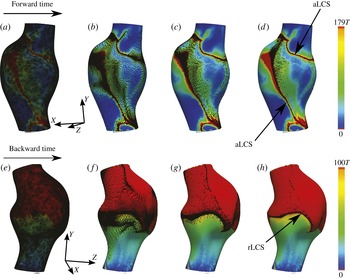
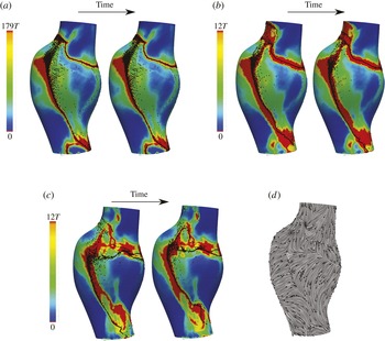
WSS exposure time (a–d) and WSS residence time (e–h) plots in first AAA model. Forward time trajectories are superimposed on the exposure time field, and backward time trajectories are superimposed on the residence time field. The forward and backward trajectories aggregate to attracting and repelling WSS LCS, respectively. Time
 $T=0.75~\text{s}$
is the cardiac cycle of the patient. The absolute time instances shown correspond to
 $t=0$
(a,e),
 $t=27T$
(b,f),
 $t=61T$
(c,g) and
 $t=100T$
(d,h).

The effect of diffusion on near-wall transport is also ignored. A simple dimensional analysis shows that the diffusion in the wall-normal direction is more significant than the streamwise diffusion. The normal diffusion in a Lagrangian framework can be modelled with a random walk approach (Ghosh et al. Reference Ghosh, Leonard and Wiggins1998),
 $$\begin{eqnarray}\displaystyle \left.\begin{array}{@{}c@{}}{\it\delta}n(t+{\rm\Delta}t)={\it\delta}n(t)+{\it\zeta},\\ {\it\zeta}\sim \mathscr{N}(0,2D{\rm\Delta}t),\end{array}\!\!\right\} & & \displaystyle\end{eqnarray}$$
where
 $D$
is the mass diffusion coefficient,
 ${\rm\Delta}t$
is the integration time step and
 ${\it\zeta}$
is a random variable determined from a Gaussian distribution, with zero mean and variance of
 $2D{\rm\Delta}t$
. In order to model the wall-normal transport effects considered by (2.5) and (2.6), trajectories were confined to stay on the wall surface; however, their wall-normal distance was tracked by these equations. Therefore, at each time step the trajectories experience a slightly different value of
 ${\it\delta}n$
, which contributes to a different value for near-wall velocity
 $\boldsymbol{u}_{{\rm\pi}}$
(see (2.2)) in addition to the inherent spatial and temporal change of the vector field. The wall-normal transport was tracked until the trajectory left a near-wall threshold (
 ${\it\delta}n_{\mathit{max}}$
), whereby the trajectory was assumed to be out of the near-wall flow region where this model holds and the integration was terminated.
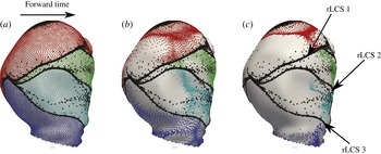
Three repelling WSS LCS are formed from backward time integration of WSS trajectories (black circles). These LCS mark the boundary of four different near-wall regions. Trajectories starting in each of these regions are coloured differently, and are shown to have different fates. The second patient is shown in this figure. The time instances shown correspond to
 $t=0$
(a),
 $t=34T$
(b) and
 $t=100T$
(c). Time
 $T=0.95~\text{s}$
is the cardiac cycle of this patient.

The near-wall distance
 ${\it\delta}n$
remains to be chosen. This distance needs to be chosen within the concentration boundary layer thickness
 ${\it\delta}_{c}$
. To approximate this, the order of magnitude of the momentum boundary layer thickness
 ${\it\delta}$
was evaluated from inspection of the thickness of the high-vorticity region near the wall. The concentration boundary layer thickness was subsequently estimated using
 ${\it\delta}/{\it\delta}_{c}=Sc^{1/3}$
(Truskey, Yuan & Katz Reference Truskey, Yuan and Katz2004). A mass diffusion coefficient of
 $D=5\times 10^{-6}~\text{cm}^{2}~\text{s}^{-1}$
was used, which approximates the diffusivity of chemicals and proteins in blood. The kinematic viscosity for blood was set to
 ${\it\nu}=0.0377~\text{cm}^{2}~\text{s}^{-1}$
, which gives
 $Sc={\it\nu}/D\approx 7500$
. Using the above estimates, the concentration boundary layer thickness was estimated as
 ${\it\delta}_{c}\approx 0.005~\text{cm}$
. Since
 ${\it\delta}n$
should be chosen within
 ${\it\delta}_{c}$
, a value
 ${\it\delta}n=0.0014~\text{cm}$
was chosen. The sensitivity to this choice will be discussed later. The maximum near-wall region thickness
 ${\it\delta}n_{max}$
was chosen within the momentum boundary layer thickness
 ${\it\delta}$
in the region where the velocity profile was mostly linear (
 ${\it\delta}n_{max}\approx 0.05~\text{cm}$
). A smaller
 ${\it\delta}n_{max}$
was tested to ensure that the results were not sensitive to this choice.
The full continuum 3D advection–diffusion problem was solved to validate the proposed Lagrangian surface transport approach. The advection–diffusion equation is written as
 $$\begin{eqnarray}\frac{\partial c}{\partial t}+\boldsymbol{u}\boldsymbol{\cdot }\boldsymbol{{\rm\nabla}}c=D{\rm\nabla}^{2}c,\end{eqnarray}$$
where
 $c$
is a non-dimensional concentration,
 $\boldsymbol{u}$
is the velocity and
 $D$
is the mass diffusivity as above. A Neumann boundary condition of
 $\partial c/\partial n=10~\text{cm}^{-1}$
was prescribed at the no-slip wall representing a uniform flux of concentration. The inlet and outlet boundary conditions were set to
 $c=0$
. Zero Dirichlet outlet boundary condition was preferred to zero Neumann boundary condition, owing to the presence of reverse flow. The outlet boundary was extended to ensure minimal influence of the outlet boundary condition. A finite element method was used to solve the equation using the streamline upwind/Petrov–Galerkin (SUPG) formulation (Brooks & Hughes Reference Brooks and Hughes1982; Bazilevs et al.
Reference Bazilevs, Calo, Tezduyar and Hughes2007), implemented in the FEniCS package (Logg, Mardal & Wells Reference Logg, Mardal and Wells2012). Second-order tetrahedral elements were used with an edge size of 0.1 cm in the interior and a boundary layer mesh with next-to-wall edge size of
 $6.6~{\rm\mu}\text{m}$
in order to resolve the concentration boundary layer. The simulation was run for 60 cardiac cycles until the surface concentration reached steady state.
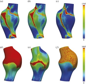
The effect of diffusion (c,f) and normal flow (b,e) on WSS exposure time (a–c) and WSS residence time (d–f). Time
 $T=0.75~\text{s}$
is the cardiac cycle of the patient. Different views of the first patient are shown in this figure.

3. Results
Figure 2 shows the WSS exposure time and WSS residence time fields in the first AAA model. Forward and backward time WSS trajectories are shown. In forward time (figure 2 a–d), WSS trajectories are seen to cluster towards distinct curves, which identify attracting WSS LCS. Trajectories remain in the vicinity of the attracting LCS for a long time, and therefore the WSS exposure time is high in such regions. Moreover, the attracting LCS demonstrates little motion over time, which causes the region of high exposure time (red region in figure 2) to be confined to narrow bands. In backward time (figure 2 e–h), WSS trajectories cluster to distinct curves, which identify a repelling WSS LCS. In this case the repelling LCS marks the boundary between the trajectories that eventually leave the domain, and those that remain in the near-wall region for a long time (high-residence-time region).
WSS exposure time contours with the attracting WSS LCS (indicated by particle clustering) for different values of
 ${\it\delta}n$
in the first patient:
 ${\it\delta}n=0.0014~\text{cm}$
(a), 0.02 (b), 0.04 (c). Two different time instants are shown to visualize the extremes in temporal displacement of the LCS. The limiting streamlines of the TAWSS vector field are also shown (d), with normalized arrows showing the direction of WSS vectors. For smaller
 ${\it\delta}n$
, the attracting LCS demonstrate less movement and are well approximated by the unstable manifolds of the TAWSS vector field. For larger
 ${\it\delta}n$
, near-wall transport, and hence WSS LCS, become more unsteady. Time
 $T=0.75$
s is the cardiac cycle for the patient. The two time instants shown differ by
 $2T$
.

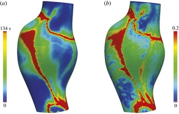
Comparison of WSS exposure time (
 $\text{WSS}_{ET}$
) (a) with the non-dimensional surface concentration (b) obtained from the corresponding 3D continuum advection–diffusion equation.

Figure 3 further demonstrates the role of the WSS LCS in organizing near-wall transport. The second patient is shown in this figure, owing to interesting WSS LCS patterns. Three repelling WSS LCS, indicated by clustering of black tracers, divide the surface into four regions. Additional tracers are seeded and coloured based on their initial position with respect to these regions. Upon advection of the coloured sets of tracers, it is seen that the trajectories starting in any of these four regions move collectively towards a different location in forward time. Namely, the repelling WSS LCS indicate boundaries between different basins of attraction for near-wall species.
The effect of diffusion and normal velocity on near-wall transport was modelled as described above and the results are shown in figure 4. The region of high WSS exposure time formed by the attracting WSS LCS remains robust with respect to these effects (figure 4 a–c). Diffusion causes some of the trajectories to leave the near-wall domain in long integration times, and therefore the exposure time is generally reduced, although the same features persist. Residence time results (figure 4 d–f) are more sensitive to diffusion and normal velocity effects. Diffusion causes trajectories to randomly leave the region of high residence time, and in general more noisy and lower-residence-time values are observed. However, the boundary between the regions of high and low residence times persists. Introduction of normal velocity leads to more dramatic change in the spatial distribution of residence time. This is for two reasons. First, the effect of normal flow is spatially dependent; in regions with large negative WSS divergence, tracers will more quickly escape from the near-wall region. Second, residence time, by its definition, is more sensitive to individual tracers leaving the near-wall region. Alternatively, exposure time depends on the collective behaviour of trajectories and is therefore less sensitive to this influence.
Next we consider the effect of different choices for
 ${\it\delta}n$
on the results, as shown in figure 5. We note that the dynamic variation of
 ${\it\delta}n$
is tacitly considered in the results of figure 4. However, our goal here is to demonstrate more directly the underlying relationship of the flow behaviour to near-wall distance. For small values of
 ${\it\delta}n$
(figure 5
a), the WSS LCS is almost stationary, fluctuating in a very narrow region of high WSS exposure time. The reason for this quasi-steady behaviour is that, very close to the wall, the WSS trajectories have a small velocity, thus have small displacements during one cardiac cycle, which is the time scale of flow unsteadiness. Subsequently, the near-wall transport becomes quasi-steady with the time-average (TA) WSS vector governing transport. Indeed, upon inspection of the limiting streamlines computed from the TAWSS vector field (figure 5
d), it can be observed that the attracting WSS LCS coincide with unstable manifolds of fixed points in the TAWSS vector field for small values of
 ${\it\delta}n$
. For larger values of
 ${\it\delta}n$
(figure 5
b,c), it can be seen that the WSS LCS demonstrate increasing fluctuation with an increase in
 ${\it\delta}n$
, as near-wall convective transport becomes less stationary. However, for large
 $Sc$
, as long as
 ${\it\delta}n$
is within
 ${\it\delta}_{c}$
, the WSS LCS change modestly, and the WSS exposure time and residence time features are persistent.
To test the validity of using the first-order near-wall velocity approximation to integrate near-wall particle transport, figure 6 compares the WSS exposure time derived from the surface transport model, and the surface concentration obtained from the full 3D advection–diffusion solution. The spatially averaged Sherwood number
 $Sh=(\partial c/\partial n)d/(C_{s}-C_{i})$
, where
 $d$
is the maximum aneurysm diameter,
 $C_{s}$
is the (spatially averaged) surface concentration and
 $C_{i}=0$
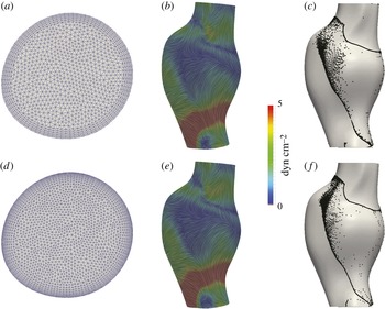
is the inlet concentration, was found to be 387. Relative agreement can be observed between the main features (identified hot spots) using the two approaches, validating the surface-based Lagrangian approach. To establish convergence of the numerical results, figure 7 shows a comparison of the baseline TAWSS streamlines and WSS LCS to those derived from a Navier–Stokes solution using a finer mesh with next-to-wall edge size of
 $100~{\rm\mu}\text{m}$
. Relatively minor changes in the structures are observed, indicating adequate near-wall resolution of the flow field solution.
Comparison of the TAWSS streamlines (b,e) and attracting LCS (aLCS) (c,f) obtained from the original mesh (a) (next-to-wall edge size
 $200~{\rm\mu}\text{m}$
) to a finer mesh (d) (next-to-wall edge size
 $100~{\rm\mu}\text{m}$
) in the first patient. The TAWSS streamlines are coloured based on the TAWSS vector magnitude.

4. Discussion
In this study the role of Lagrangian WSS structures on organizing the near-wall transport of high-
 $Sc$
flows was investigated in the context of blood flow in abdominal aortic aneurysms. It was shown that the attracting and repelling WSS LCS act as templates of near-wall transport. The applicability of this approach relies on the existence of a thin concentration/thermal boundary layer. Using
 ${\it\delta}$
to scale the wall-normal distance, the relative error in neglecting the higher-order terms in (2.2) is
 $O({\it\delta}n/{\it\delta})$
. Because
 ${\it\delta}n$
is chosen to be of the same order as
 ${\it\delta}_{c}$
, the relative error in the linear approximation is
 $O({\it\delta}_{c}/{\it\delta})$
. A relative error of 10 % gives
 $Sc\approx 1000$
. Therefore, the current approach may give reasonable results for
 $Sc$
or
 $Pr$
numbers of
 $O(10^{3})$
or higher (in the examples shown,
 $Sc\approx 7500$
). We note however that the second-order term scales with WSS divergence; thus the near-wall transport model can break down in locations of high WSS divergence (cf. figure 4).
Tracers are seeded near the wall (
 ${\it\delta}n=7~{\rm\mu}\text{m}$
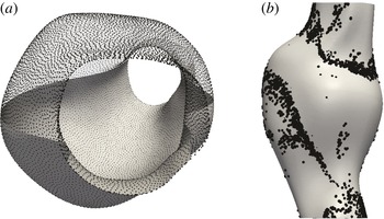
) and integrated in forward time using the first patient model: (a) shows initial tracer seed locations, and (b) shows the emerging near-wall structures after sufficient forward 3D integration. (Particles on right are enlarged to become visual through the surface.)

It has been shown that for
 $Sc\gtrsim O(10^{3})$
mass transfer resulting from unsteady blood flow was similar to that obtained from the time-averaged components (Ma, Li & Ku Reference Ma, Li and Ku1994). Our results are consistent and provide further explanation. Two different time scales govern the near-wall transport. The time scale for variations in the base flow (one cardiac cycle) is much smaller than the time scale for effective transport of near-wall species (several cardiac cycles), implying that near-wall transport is quasi-steady. It is important to keep in mind that in complex flows a time-dependent flow solution is still needed, as the time-averaged WSS field obtained from the time-dependent flow can be different from the WSS field obtained from a steady simulation with a time-averaged inflow. For the flow conditions considered in this study, we verified that using the TAWSS vector as a steady vector produced nearly identical
 $\text{WSS}_{ET}$
results to the corresponding unsteady WSS vector field. Our results also demonstrated that the quasi-steady behaviour of near-wall transport led to the conforming of the WSS LCS with the stable/unstable manifolds of the TAWSS vector field. Moreover, Shariff, Pulliam & Ottino (Reference Shariff, Pulliam and Ottino1991) have shown that stable/unstable manifolds in the velocity field emerge from critical points of the time-averaged WSS field in periodic two-dimensional flows. Therefore, the relation between WSS critical points and their invariant manifolds with the core flow features can provide insight into the basis of near-wall transport.
For high-
 $Sc$
, as long as
 ${\it\delta}n$
was chosen within the concentration boundary layer, the exact choice did not significantly affect the qualitative behaviour of the WSS LCS, WSS exposure time and residence time fields. We note that a decrease in
 $Sc$
yields a larger concentration boundary layer thickness, and subsequently more unsteadiness in near-wall transport manifested in the temporal variations of WSS LCS. In the case of smaller
 $Sc$
flows, a higher-order representation of the near-wall flow by means of a series expansion (Perry & Chong Reference Perry and Chong1986) may be employed to accurately model the near-wall transport with a larger
 ${\it\delta}n$
. In this case, depending on
 $Sc$
, it is likely that the trajectories closer to the wall will be controlled by the time-averaged WSS vector field manifolds, and trajectories further away from the wall will be subject to unsteadiness around these manifolds (cf. figure 5).
While one may use the full 3D velocity field to track near-wall tracers, this can be difficult to implement. For validation, we seeded tracers
 ${\it\delta}n=7~{\rm\mu}\text{m}$
from the wall and integrated them forward in time using the full 3D flow field until coherent structures were formed near the wall as shown in figure 8. It can be observed that tracers accumulate near the same attracting WSS LCS as shown in figure 2. However, in using the 3D velocity field for integrating near-wall tracers, small errors in numerical integration are more easily amplified. Namely, such errors result in (1) increases in
 ${\it\delta}n$
causing higher normal velocities and tracers leaving the near-wall region prematurely, or (2) decreases in
 ${\it\delta}n$
causing tracers to stick to, or penetrate, the wall. Over the long integration times needed to understand near-wall transport, the accuracy of near-wall integration can become significantly impaired due to these effects. Alternatively, the surface integration method provides a more efficient approach, while maintaining accuracy, as for example demonstrated by the agreement between
 $\text{WSS}_{ET}$
and the surface concentration obtained from solving the 3D continuum advection–diffusion equation (cf. figure 6).
For most vascular applications, the emergent WSS LCS patterns will be largely dependent on the vascular geometry and Reynolds and Womersley numbers, as these factors most influence flow topology. Indeed, Gopalakrishnan, Pier & Biesheuvel (Reference Gopalakrishnan, Pier and Biesheuvel2014) have shown that small changes in the AAA geometry can significantly affect the WSS distribution, and changes in the curvature of the vessel wall have also been shown to affect WSS (Siggers & Waters Reference Siggers and Waters2008). In the current study we demonstrated results in two patient geometries; however, we also performed similar simulations in a total of six patient geometries and observed similar WSS LCS structures influencing the observed near-wall concentration fields. Thus, the indication that Lagrangian WSS structures can provide a template for near-wall transport appears to hold generally over widely varying geometrical models.
The inlet flow waveforms used in this study were patient-specific resting waveforms obtained from phase contrast magnetic resonance measurements. We have performed preliminary study on the effect of simulated exercise flow conditions (increased Reynolds and Womersley numbers, as modelled in Arzani et al. (Reference Arzani, Les, Dalman and Shadden2014a )) on WSS LCS, and observed that the quasi-steady behaviour of near-wall transport can break down due to the higher WSS magnitudes. In addition, pulsatile blood flow may have some cycle-to-cycle variations due to transient effects from the fluid mechanics or physiology. In this study we assumed a periodic WSS vector field to generate WSS trajectories. Depending on the Reynolds and Womersley numbers, the intercycle variations in the flow field can break down the quasi-steady behaviour of the WSS LCS, leading to greater unsteadiness in the near-wall transport. Under such conditions the WSS LCS may demonstrate time-dependent behaviour and deviate from the stable/unstable manifolds of the TAWSS field. Additional considerations that remain to be studied are that higher WSS divergence magnitudes typically observed under exercise conditions, as well as physiological deformation of the vessel wall due to wall compliance, may increase transport normal to the vessel wall in the boundary layer. To visualize the WSS LCS in this study, we relied on a simple advection of tracers. Alternatively, one could compute the finite-time Lyapunov exponents on a non-Euclidean manifold to visualize the LCS (Lekien & Ross Reference Lekien and Ross2010). The simple approach employed here is nonetheless able to identify the more prominent LCS, which affect the concentration pattern on the vessel surface.
The current study provides a framework for understanding the mechanisms underlying mass/heat flux at a no-slip wall in disturbed high-
 $Sc$
or high-
 $Pr$
flows. In particular, attracting WSS LCS determine patterns of high species concentration, and repelling WSS LCS mark the boundaries of different basins of attraction. Therefore, the WSS LCS provide a template for the distribution and evolution of wall-generated species. Recently, Nguyen, Srinivasan & Papavassiliou (Reference Nguyen, Srinivasan and Papavassiliou2015) have demonstrated the separation between near-wall species with different
 $Sc$
. This separation could also happen due to the partitioning effect of the repelling WSS LCS as demonstrated in figure 3. From a design perspective, it would be interesting to manipulate these structures to obtain a WSS pattern with a desired outcome of wall concentration or temperature distribution, in similar fashion to Hubble, Vlachos & Diller (Reference Hubble, Vlachos and Diller2013), who investigated the effect of vortical structures near the boundary layer on heat transfer augmentation. Finally, the bearing of these structures on near-wall transport of turbulent flows remains to be investigated.
Acknowledgements
This work was supported by the NIH National Heart, Lung, and Blood Institute (grant no. HL108272) and the National Science Foundation (grant no. 1354541). A.M.G. gratefully acknowledges the support from ‘MatComPhys’ under the European Research Executive Agency FP7-PEOPLE-2011-IEF framework. The authors are thankful to K. B. Hansen for assistance with the advection–diffusion solver.