


1. Introduction
The reduction of turbulent skin-friction drag has been a subject of major interest in the fluid mechanics community for decades, due to the potential to lead to lower fuel consumption, noise and pollutants emissions in numerous industrial and technological applications.
Amongst the active flow-control techniques, namely those requiring an external energy input, significant reductions of turbulent skin-friction drag have been achieved by applying spanwise sinusoidal wall oscillations. This drag-reduction effect was first reported in a fully developed turbulent channel flow by Jung, Mangiavacchi & Akhavan (Reference Jung, Mangiavacchi and Akhavan1992) via direct numerical simulations (DNS). They studied the response of wall-bounded turbulence to different periods of spanwise wall oscillations,  $T^+_{osc}$, ranging from 25 to 500, and computed a maximum 40 % decrease of the wall-shear stress when the turbulence intensity was suppressed the most for a period of
 $T^+_{osc}=100$ (the superscript + herein indicates scaling by the wall-friction velocity).
Baron & Quadrio (Reference Baron and Quadrio1996) confirmed the drag-reduction results of Jung et al. (Reference Jung, Mangiavacchi and Akhavan1992) by DNS, and first considered the energy balance of a turbulent channel flow with spanwise wall oscillations by fixing the oscillating period for  $T^+_{osc}=100$ and changing the amplitude of the oscillation. A positive net energy balance, computed by subtracting the power spent to move the wall from the power saved through drag reduction, was found for small wall-velocity amplitudes. Choi, DeBisschop & Clayton (Reference Choi, DeBisschop and Clayton1998) investigated experimentally a fully developed turbulent boundary layer subjected to spanwise wall oscillations. They confirmed the results of the previous DNS studies, and a maximum skin-friction reduction of
 $45\,\%$ was measured at a distance of five boundary-layer thicknesses downstream of the start of oscillating section of the wall. Quadrio & Ricco (Reference Quadrio and Ricco2004) also employed DNS to further investigate the power saved and the power required by the spanwise wall oscillations in a turbulent channel flow. The maximum drag-reduction margin of
 $45\,\%$ and the maximum net energy saving of
 $7\,\%$ were both computed for
 $T^+_{osc}=125$. The drag-reduction effect and the net balance were improved by Quadrio, Ricco & Viotti (Reference Quadrio, Ricco and Viotti2009) and Quadrio & Ricco (Reference Quadrio and Ricco2011) by the use of streamwise-travelling waves of spanwise wall velocity. Backward-travelling waves always generated drag reduction, while forward-travelling waves led to drag increase when the phase speed of the waves was comparable with the convection velocity of the near-wall turbulent structures. Waves travelling forwards with a small phase speed led to a maximum drag-reduction margin of
 $48\,\%$ and a maximum net power saving of
 $23\,\%$. The discussed studies confirm that spanwise wall forcing methods are promising because of the large drag-reduction margin and positive net energy balance, but their direct implementation in technological systems, such as over aircraft wings or fuselage, is undoubtedly prohibitive because of the impractical requirement of the fast and large-scale motion of the surface.
An alternative active method for drag reduction without moving walls is synthetic jets (Glezer & Amitay Reference Glezer and Amitay2002), which involve localized zero-net-mass periodic wall transpiration. Inspired by the wall-oscillation technique, studies have focused on the alteration of wall turbulence by synthetic jets along the spanwise direction. Iuso et al. (Reference Iuso, Onorato, Spazzini and di Cicca2002) and Iuso & Di Cicca (Reference Iuso and Di Cicca2007) demonstrated experimentally that local skin-friction reductions as large as  $30\,\%$ can be obtained in a turbulent channel flow with pairs of jets. These jets, ejecting from ten holes drilled through the upper channel wall and produced by a compressed air supply, were inclined alternately at angles
 ${\pm }45^{\circ }$. The holes were aligned along the spanwise direction, and the measurement devices were positioned downstream of the jet-injection section. Iuso et al. (Reference Iuso, Onorato, Spazzini and di Cicca2002) conjectured that the drag-reduction effect was achieved by the combined action of the pairs of counter-rotating streamwise vortices generated by the jets, and the local flow separation close to the location of the jet orifices. Tay et al. (Reference Tay, Herberg, Onorato and Tsai2007) also forced the wall turbulence in a wind tunnel by jets ejecting from holes inclined at angle
 $45^{\circ }$, but air was released continuously from the holes. A local drag-reduction margin of
 $50\,\%$ was measured under the optimal condition. Cannata & Iuso (Reference Cannata and Iuso2008) and Cannata, Cafiero & Iuso (Reference Cannata, Cafiero and Iuso2020) continued the work of Iuso & Di Cicca (Reference Iuso and Di Cicca2007) and forced the near-wall turbulence by synthetic jets ejecting from ten tubes installed on the top part of the two vertical channel walls. The jet holes were aligned in the streamwise direction, and the jet forcing was spanwise and tangential to the upper channel wall. The peak reduction of the local mean drag was
 $22\,\%$. Using DNS, Yao, Chen & Hussain (Reference Yao, Chen and Hussain2018) mimicked the bulk spanwise motion caused by the spanwise synthetic jets by imposing a body force in the equations of motion. Drag reduction was achieved and the net power saving was
 $17\,\%$ in the optimal case.
Spanwise jets have also been generated near the wall by pulsed-DC plasma actuation. The aerodynamics research group at the University of Notre Dame demonstrated that this technique can lead to turbulent drag-reduction margins as large as 75 % (Corke & Thomas Reference Corke and Thomas2018; Thomas et al. Reference Thomas, Corke, Duong, Midya and Yates2019). The plasma-induced jet velocity was generated in extremely short pulses by electrodes located at about 1000 wall units apart along the span. The low power spent led to a positive net power saved. Through near-wall plasma forcing, Hehner, Gatti & Kriegseis (Reference Hehner, Gatti and Kriegseis2019) and Hehner et al. (Reference Hehner, Gatti, Mattern, Kotsonis and Kriegseis2020) produced a well-defined oscillating boundary layer that could be utilized for near-wall flow control. Ricco, Skote & Leschziner (Reference Ricco, Skote and Leschziner2021) reviewed the existing literature on turbulent drag reduction via spanwise actuation, including wall motion, plasma body forces and synthetic jets.
In previous studies, jets have led to drag reduction locally in the proximity of the jet holes, but a distributed reduction of the wall-shear stress over the entire surface has not been achieved. Furthermore, only experimental studies exist on drag reduction by spanwise-oriented synthetic jets, and the mechanical actuators for the generation of jets have never been modelled. The objective of the present study is therefore to investigate the effect of spanwise-oriented jets by numerical means in order to achieve drag reduction over an extended portion of the surface bounding the turbulence. To reach our objective, we employ a novel technique based on jet sheets extending continuously along the streamwise direction, instead of localized jets from orifices that have not been shown to lead to distributed drag reduction. The wall-tangential jet sheets force a fully developed turbulent channel flow at friction Reynolds number  $\mbox {{Re}}_\tau =180$, and are confined in the very proximity of the wall. They eject from thin slots parallel to the channel walls, oscillating sinusoidally in time.
As the jet sheets are an active flow-control method, power is required to operate them. In order to calculate the power spent, it is therefore fundamental to model accurately the actuators that generate the jet sheets. An actuator is modelled as an oscillating piston located in a cavity underneath the channel walls. The flow generated by the actuators inside the cavity is computed numerically, and the power spent is accounted for in the power budget for the computation of the net power saved. The control method is herein referred to as wall-tangential synthetic jet sheets (SJS).
In § 2, the flow system is described and the numerical procedures are presented. Sections 3.1, 3.2 and 3.3 discuss the results on the drag-reduction effects and the turbulent-flow physics, while the cavity flow and the power performance of the SJS actuator are studied in § 3.4. Conclusions are drawn in § 4.
2. Flow system and numerical procedures
In this section, the channel and the actuators are described in § 2.1, and the averaging procedures are discussed in § 2.2. Appendix A presents a validation study of the numerical computations.
2.1. Channel flow and actuators
We study numerically a fully developed turbulent channel flow of air driven at a constant mass flow rate and at friction Reynolds number  $\mbox {{Re}}_\tau =u^*_\tau h^*/\nu _c^*= 180$, where
 $h^*$ is the half-channel height, and
 $u^*_\tau = \sqrt {\tau ^*_w/\rho _c^*}$ is the wall-friction velocity (the superscript * herein denotes dimensional quantities). The quantities
 $\tau ^*_w$,
 $\nu _c^*$ and
 $\rho _c^*$ are the space- and time-averaged wall-shear stress in the uncontrolled case, the kinematic viscosity and the density of air, respectively. Quantities that are not marked by any symbol are scaled in outer units, i.e. by
 $h^*$ and
 $U^*_p$, the centreline velocity of the laminar parabolic Poiseuille flow at the same mass flow rate, and quantities marked by the superscript ‘+’ are non-dimensionalized in wall units, i.e. by
 $\nu _c^*$ and
 $u^*_\tau$ of the uncontrolled case.
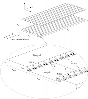
Figure 1 shows the flow system, where  $L_x$,
 $L_y$ and
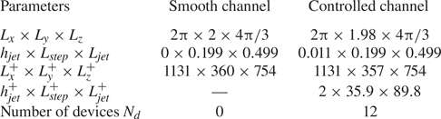
 $L_z$ are the lengths of the computational domain in the streamwise, wall-normal and spanwise directions, respectively. The flow conditions and dimensions of the flow cases discussed in the main text are given in table 1. Appendix B presents additional flow cases. On each wall, six steps of height
 $h_{{jet}}$ are aligned along the streamwise direction. The SJS eject from slots located at both sides of the steps. The surface of the step is named ‘step wall’, and the surface between two slots is named ‘jet wall’. The spanwise width of a step wall is
 $L_{{step}}$, and the spanwise width of a jet wall is
 $L_{{jet}}$. The length
 $L_{jet}^+$ has been chosen to be comparable with the spacing of the low-speed streaks in wall-bounded turbulence (about 100 units), and
 $L_{step}^+$ has been chosen as small as possible not to disrupt the flat-wall standard geometry, but wide enough so that it could accommodate realistically the channels underneath the steps, through which air flows to discharge into the main turbulent flow. A suction/blowing type boundary condition is applied at the slot exits. The skin friction of the flow through the smooth channel without steps on the walls is taken as the reference value for the computation of the drag reduction. The terminology ‘SJS off’ refers to the channel flow with steps but without SJS actuation, while ‘SJS on’ refers to the channel flow with steps and activated SJS.
Schematic of the channel flow with SJS. The velocity profiles are for  $\beta = 0^{\circ }$.

Flow conditions and dimensions of the flow cases discussed in the main text. Appendix B presents additional flow cases.

The components of the SJS velocity vector at the slot exits are
 $$\begin{gather} u_{{jet}} = U_{{jet}} \sin \beta \sin \left( \frac{2 {\rm \pi}t}{T_{osc}} \right), \end{gather}$$
 $$\begin{gather}v_{{jet}} = 0, \end{gather}$$
 $$\begin{gather}w_{{jet}} = U_{{jet}} \cos \beta \sin \left( \frac{2 {\rm \pi}t}{T_{osc}} \right), \end{gather}$$
where  $u$,
 $v$ and
 $w$ are the velocity components along the streamwise, wall-normal and spanwise directions, respectively. The angle
 $\beta$ of the SJS ejection is defined with respect to the spanwise direction, and the period of the oscillation is
 $T^+_{osc}=125$. The SJS work in pairs as shown in figure 1, i.e. the SJS velocities are
 $u_{jet, side1} = -u_{jet, side2}$ and
 $w_{jet, side1} = w_{jet, side2}$.
The velocity profile  $U_{{jet}}$ follows a parabolic function (You, Wang & Moin Reference You, Wang and Moin2006)
 \begin{equation} U_{{jet}} = U_{jet, peak}\left[ 1- \left(\frac{2y_{jet}}{h_{jet}} - 1\right)^2 \right],\quad 0 \leq y_{jet} \leq h_{jet}, \end{equation}
where  $U_{jet, peak}$ is the peak velocity, and
 $y_{jet}$ is the wall-normal distance from the jet wall. The peak velocity is
 $U^+_{{jet, peak}}=27$ for the main cases studied. The Reynolds number and the Strouhal number of the SJS flow are
 $\mbox {{Re}}_{jet} = U^*_{jet,peak} h^*_{jet} / \nu ^*_c =54$ and
 $St = h^*_{jet} / (U^*_{jet,peak} T^*_{osc})=0.0006$. The Mach number based on the channel flow bulk velocity and the speed of sound at the reference temperature is 0.21. The Mach number based on the peak SJS velocity and the speed of sound at the reference temperature is 0.35.
2.2. Averaging procedures
The case with the SJS off is used as the initial flow for the SJS simulations. When this turbulent flow has reached fully developed statistically convergent conditions, the SJS are switched on. The flow in turn evolves to a new drag-reducing or drag-increasing regime. The averaging procedures are performed on a quantity after discarding the transient from the beginning of the SJS actuation, when the flow has reached fully developed conditions.
The flow within the computational domain is statistically periodic along the spanwise direction. The minimal geometrical flow unit that repeats itself along the spanwise direction is  $L= L_{step}+L_{jet}$. As the flow is statistically homogeneous along
 $x$, the spatial ensemble and streamwise average of a quantity
 $q$ is
 \begin{equation} [q]_e(y,z_e,t) = \frac{1}{n_z L_x} \sum_{n_z = 0}^{N_z-1} \int_0^{L_x} q ( x,y,z_e+n_z L,t )\, \mathrm{d}\kern 0.06em x, \end{equation}
where  $0 \leq z_e \leq L$ is the ensemble spatial coordinate, and
 $N_z$ is the number of minimal geometrical units in the computational domain.
As the SJS forcing is sinusoidal with period  $T_{osc}$, the flow is statistically periodic with the same period. The phase ensemble average is
 \begin{equation} \langle q \rangle(y,z_e,\varphi) = \frac{1}{N_{osc}}\sum_{n_{osc}=0}^{N_{osc}-1} [q]_e \left[y,z_e,\left(\frac{\varphi}{2{\rm \pi}}+n_{osc} \right) T_{osc} \right], \end{equation}
where  $N_{osc}$ is the number of oscillating periods, and
 $\varphi$ is the phase,
 \begin{equation} \varphi = \frac{2 {\rm \pi}\tau}{T_{osc}}\quad (0 \leq \tau \leq T_{osc}). \end{equation}
The ensemble and time average over a time interval  $T$ is
 \begin{equation} \bar{q}(y,z_e) = \frac{1}{T}\int_0^{\rm T} [q]_e(y,z_e,t)\,\mathrm{d} t. \end{equation}
A triple decomposition is defined as
 \begin{equation} q(x,y,z,t) = \bar{q}(y, z_e) + \tilde{q}(y, z_e, \varphi) + q''(x,y,z,t), \end{equation}
where
 \begin{equation} \tilde{q}(y, z_e, \varphi) = \langle q \rangle(y, z_e, \varphi) - \bar{q}(y, z_e) \end{equation}
is the periodic fluctuation induced by the SJS, and
 \begin{equation} q''(x,y,z,t) = q(x,y,z,t) - \langle q \rangle(y, z_e, \varphi) \end{equation}
denotes a purely turbulent quantity. The total fluctuation is defined as
 \begin{equation} q'(x,y,z,t) = \tilde{q}(y, z_e, \varphi) + q''(x,y,z,t). \end{equation}
The total Reynolds shear stresses are computed by the total fluctuations  $\overline {u'v'}$, while the Reynolds shear stresses involving only the turbulent fluctuations are computed as
 $\overline {u''v''}$. The scaled wall-shear stress is
 \begin{equation} C_f(x,z,t) =\frac{2 \mu_c^*}{\rho_c^* U_b^{*2}} \left.\frac{{\partial} u^*(x,y,z,t)}{{\partial} y^*}\right\lvert_{y^*=0}, \end{equation}
where  $\mu _c^*$ is the dynamic viscosity of air, and
 $U_b^*$ is the bulk mean velocity. The spatially averaged skin-friction coefficient is
 \begin{equation} \hat{C}_f(t) =\frac{1}{ L_z L_x} \int_0^{L_z}\int_0^{L_x} C_f(x,z,t)\,\mathrm{d}\,x\,\mathrm{d} z. \end{equation}
The time and spatially ensemble averaged skin-friction coefficient in the period  $T_{osc}$ is
 \begin{equation} \overline{C}_f(z_e) = \frac{1}{N_z T_{osc} L_x} \sum_{n_z = 0}^{N_z-1} \int_0^{T_{osc}} \int_0^{L_x} C_f ( x,z_e+n_z L,\tau )\, \mathrm{d}\kern 0.06em x\,\mathrm{d} \tau. \end{equation}
The phase and spatially ensemble averaged skin-friction coefficient is
 \begin{equation} \langle C_f \rangle(z_e, \varphi) = \frac{1}{N_z N_{osc} L_x} \sum_{n_z = 0}^{N_z-1} \sum_{n_{osc}=0}^{N_{osc}-1} \int_0^{L_x} C_f \left[ x,z_e+n_z L, \left(\frac{\varphi}{2{\rm \pi}}+n_{osc} \right) T_{osc} \right] \mathrm{d}\kern 0.06em x. \end{equation}
The level of gross drag reduction is defined as
 \begin{equation} \mathcal{R}(\%)= 100(\%) \times \frac{[C_f]_{{smooth}} - [C_f]_{{controlled}}}{[C_f]_{{smooth}}}, \end{equation}
where  $[C_f]$ is the global skin-friction coefficient,
 \begin{equation} [C_f] =\frac{1}{T L_z L_x} \int_0^{T}\int_0^{L_z} \int_0^{L_x} C_f(x,z,t)\,\mathrm{d}\kern 0.06em x\,\mathrm{d}z\,\mathrm{d}t. \end{equation}
2.3. Numerical solver
The in-house flow solver SHEFFlow, based on and further developed from the solver by Qin & Xia (Reference Qin and Xia2008), is utilized to simulate the turbulent channel flow and the flow in the cavity underneath the channel. It solves the three-dimensional compressible Navier–Stokes equations by employing a finite volume method, a dynamic mesh formulation, and a preconditioned Roe scheme. For the spatial discretization, a fifth-order monotonic upwind scheme for conservation laws (MUSCL) scheme without any limiter functions is employed to gain a higher order of accuracy and low dissipation (Kim & Kim Reference Kim and Kim2005). A dual time step scheme is used for the temporal discretization (Weiss & Smith Reference Weiss and Smith1995). The physical-time term is discretized implicitly by a second-order-accurate, three-point-backward finite-difference scheme, while the pseudo-time derivative is driven to zero by a multistage Runge–Kutta scheme. Parallelization is achieved using the open message passing interface.
3. Results
3.1. Turbulent drag reduction
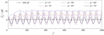
Figure 2 displays the time evolution of the spatially averaged skin-friction coefficient  $\hat {C}_f$ for different SJS angles
 $\beta$. The coefficient is strongly influenced by the SJS; it displays intense fluctuations that become periodic after two forcing periods. The oscillating period of these wall-friction fluctuations is
 $T_{{osc},\hat {C}_f}^+=62.5$, half of the period
 $T_{{osc}}$ of the SJS. The fluctuations of
 $\hat {C}_f$ depend on the SJS velocity; they are smallest for
 $\beta = 0^{\circ }$, and largest for
 $\beta = 60^{\circ }$, which means that they increase as the streamwise component of the SJS velocity vector increases up
 $\beta = 60^{\circ }$. For larger angles, the fluctuating amplitude does not grow monotonically with the SJS angle; the case
 $\beta = 75^{\circ }$ has a smaller amplitude than the case
 $\beta = 60^{\circ }$. As
 $\beta$ approaches
 $90^{\circ }$, the SJS flow becomes more and more aligned along the streamwise direction, so that the area of influence of the SJS becomes smaller, leading to a small fluctuating amplitude of
 $\hat {C}_f$. The amplitude of the wall-shear stress therefore oscillates less for large
 $\beta$ values than for
 $\beta = 60^{\circ }$. When
 $\beta = 90^{\circ }$, no flow exhausts into the channel from the SJS exits because the SJS velocity vector is unrealistically parallel to the slots, thus being less able to influence the bulk flow.
Time evolution of the skin-friction coefficient for different SJS angles.

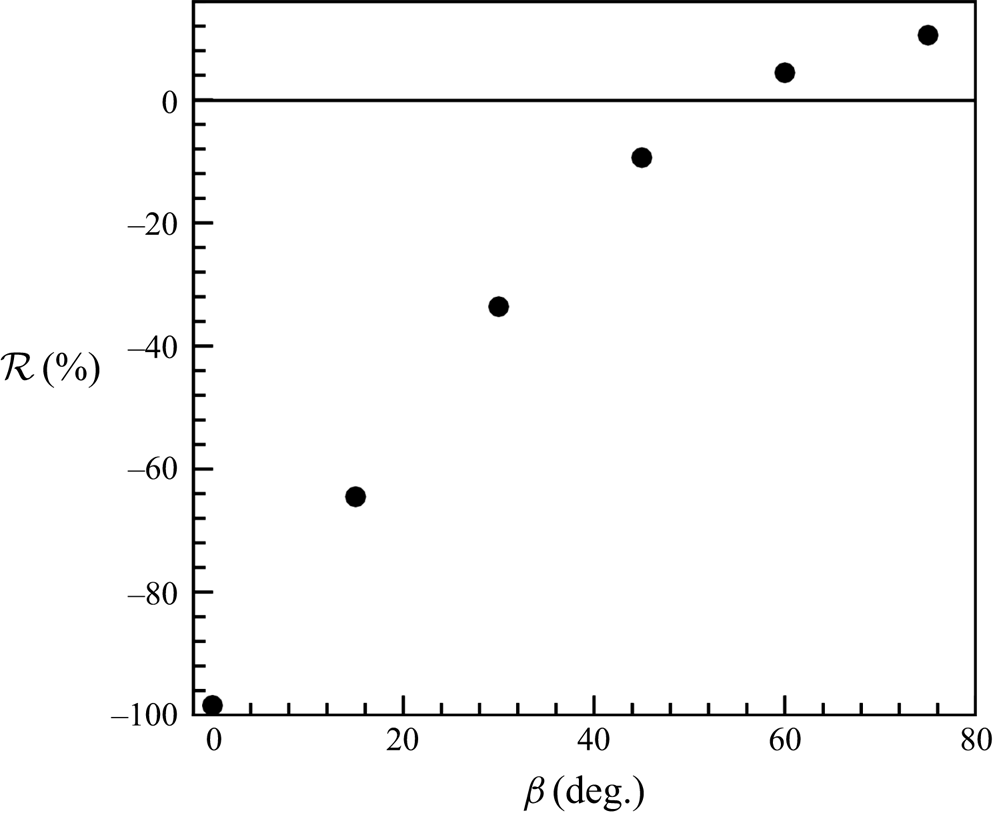
Figure 3 shows the drag-reduction margin as a function of the SJS angle. The maximum value is  $\mathcal {R}=10.5\,\%$ when
 $\beta = 75^{\circ }$. The SJS angle
 $\beta = 0^{\circ }$ gives the maximum drag increase, that is, the drag coefficient is 98.4 % larger than the coefficient of the uncontrolled channel. Interpolating the data in figure 3 leads to the estimate that SJS with
 $\beta = 54^{\circ }$ generate a flow with the same average drag as the uncontrolled flow. Appendix B discusses the effects of varying the slot height, the period of forcing, the peak SJS velocity and the distance between the slots.
Drag reduction for different SJS angles.

3.2. Mean-flow and turbulence statistics
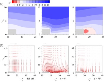
Figure 4(a) illustrates the time and spatially averaged streamwise velocity  $\overline {u}^+$ near the slots for the reference case with the SJS off, the drag-increase case for
 $\beta = 0^{\circ }$, and the drag-reduction case for
 $\beta = 75^{\circ }$. The skin-friction coefficient of the case with SJS off is
 $\hat {C}_f=8.20 \times 10^{-3}$ for the parameters in table 1, i.e.
 $0.24\,\%$ larger than that of the smooth channel,
 $\hat {C}_f=8.18 \times 10^{-3}$ (Kim, Moin & Moser Reference Kim, Moin and Moser1987). As reported in Appendix A, this difference is within the uncertainty range, estimated to be less than 1 %, which proves that the steps have a negligible influence on the skin friction for
 $h_{{jet}}^+=2$. A region of negative mean streamwise velocity is found near the slots for the case
 $\beta = 75^{\circ }$, which is not present when the SJS eject at
 $\beta = 0^{\circ }$. Although the SJS are characterized by a zero-net-mass flux at the slots, the time averaging reveals that a significant near-wall counter flow opposite to the bulk streamwise flow occurs when
 $\beta = 75^{\circ }$. No net counter flow is detected for
 $\beta = 0^{\circ }$ because no SJS flow is imposed against the bulk flow. The generation of the counter flow near the SJS slots is similar to that induced by canonical synthetic jets exhausting perpendicularly to a cross flow. In their review, Glezer & Amitay (Reference Glezer and Amitay2002) discuss several cases where synthetic jets, although characterized by a zero-net-mass flux, modify the cross flow into which they discharge and produce a displacement of its streamlines, thereby engendering a virtual change in the surface shape. In our study, the distortion of the bulk turbulent flow also occurs along the wall-normal direction as in Glezer & Amitay (Reference Glezer and Amitay2002), but the change is due to the SJS forcing, which is parallel to the walls. Increasing the SJS angle from
 $\beta = 0 ^{\circ }$, the SJS flow is directed against the main flow, producing the counter flow near the exits. When the SJS angle is large enough, the counter flow becomes a dominant effect on altering the velocity profile to reduce the near-wall velocity gradient and therefore the friction drag.
Time and spatially averaged flow near the slots on the  $y$–
 $z$ plane. (a) Contours of the averaged streamwise-velocity. (b) Vectors of the induced time-averaged flow
 $(\overline {v}^+, \overline {w}^+)$. The magnitude of the velocity vectors is equal to
 $\sqrt {\overline {v}^{+2} + \overline {w}^{+2}}$. The arrow at the top of each graph denotes the unit length for the vectors in the graph. The maximum magnitudes in the cases with the SJS off,
 $\beta = 0^{\circ }$ and
 $\beta = 75^{\circ }$, are
 $0.08$,
 $3.57$ and
 $0.56$, respectively.

Figure 4(b) shows the velocity vectors of the time-averaged cross-flow velocity components  $(\overline {v}^+,\overline {w}^+)$. A mild cross flow with clockwise rotation occurs when the SJS are off, similar to the secondary flows reported by Hwang & Lee (Reference Hwang and Lee2018) numerically and Vanderwel & Ganapathisubramani (Reference Vanderwel and Ganapathisubramani2015) experimentally for turbulent flows over longitudinal rectangular roughness elements. Hwang & Lee (Reference Hwang and Lee2018) changed systematically the spanwise distance and the width of the steps, and reported that the strength of the secondary vortices increases when the spanwise distance increases or when the width decreases. Vanderwel & Ganapathisubramani (Reference Vanderwel and Ganapathisubramani2015) also revealed that the vortical flows exist next to the roughness elements, and their strength depends on their spanwise spacing. When the spacing is comparable with the boundary-layer thickness, the secondary vortices reach their maximum strength. The presence of instantaneous secondary flows was demonstrated further by Vanderwel et al. (Reference Vanderwel, Stroh, Kriegseis, Frohnapfel and Ganapathisubramani2019), using both experiments and numerical simulations.
When the SJS are on, although the time-averaged velocity components are null at the slots, a finite time-averaged cross flow is generated by the nonlinear interaction between the SJS and the bulk streamwise flow. The intensity of this cross flow is much larger than that in the reference case with SJS off, and the rotation is anticlockwise, that is, opposite to the rotation occurring when the SJS are off. When  $\beta = 0^{\circ }$, the time-averaged SJS flow is more intense and more confined near the jet wall than in the case
 $\beta = 75^{\circ }$. The bulk of the cross flow is pushed upwards and away from the slots. The time-averaged cross flow is similar to the wall jets studied by Yao et al. (Reference Yao, Chen and Hussain2018), although in their case finite time-averaged jets are expected to form because they are generated by a steady spanwise body force.
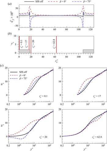
Figure 5 compares further time and spatially averaged quantities for the cases with the SJS off,  $\beta = 0^{\circ }$ and
 $\beta = 75^{\circ }$. Figure 5(a) shows the averaged scaled wall-shear stresses
 $\overline {C}_f$ along the spanwise direction. Consistently with the near-wall counter flow observed for
 $\beta = 75^{\circ }$ near the slots, the local wall-friction drag is reduced there. This result proves that the drag-reduction mechanism is different from other spanwise-forcing techniques, such as the oscillation wall (Quadrio & Ricco Reference Quadrio and Ricco2004) or the streamwise-travelling waves of spanwise wall velocity (Quadrio et al. Reference Quadrio, Ricco and Viotti2009), for which the wall-shear stress is never negative. As the case with
 $\beta = 75^{\circ }$ involves a significant oscillatory velocity component along the streamwise direction, the drag-reduction effect is akin to that reported by Zhou & Ball (Reference Zhou and Ball2008), who moved the wall obliquely with respect to the streamwise direction. They concluded that although forcing the flow purely along the spanwise direction led to the best performance, drag reduction was also found when most of the wall motion was along the streamwise direction. For
 $\beta = 0^{\circ }$, the wall-friction drag is more than six times larger than the uncontrolled value in the proximity of the slots, and the wall-shear stress is not reduced at any spanwise location. Along the central part of the jet wall, the trends of the wall-shear stress are flat and overlap in all three cases, indicating that the friction drag is unaffected along that portion of the wall because that region is too far from the SJS slots. Drag increase occurs over the step walls in both controlled cases.
Comparisons of time and spatially averaged quantities at different spanwise positions. (a) Distributions of averaged skin friction along the spanwise direction. (b) Profile positions. (c) Profiles of averaged streamwise velocity, covering the height range of a half-channel.

The profiles of the time-averaged streamwise velocity are shown in figure 5(c), and the respective spanwise locations are indicated in figure 5(b). Over the step wall at  $z_e^+ = 0.1$ and
 $17$, the large mean velocity in the controlled cases, which causes the local drag increase shown in figure 5(a), is limited only very close to the wall as the profiles show a good agreement with the uncontrolled profile at wall-normal distances
 $y^+>10$ from the step wall. The SJS with
 $\beta = 0^{\circ }$ create drag increase near the slot at
 $z_e^+ = 20$ by intensifying the mean streamwise velocity only up to
 $y^+=25$, while the reverse flow for
 $\beta = 75^{\circ }$ is confined up to
 $y^+=5$, i.e. in the viscous sublayer. At higher locations, the profiles for the controlled flows agree more closely to the uncontrolled profile, although a velocity deficit is found for
 $25< y^+<80$. In the middle of the jet wall at
 $z_e^+ = 62.8$, the three profiles overlap within the viscous sublayer, and the velocity deficit with respect to the uncontrolled case between
 $10< y^+<100$, is more pronounced than that at other spanwise locations, arguably because of the intense lift-up effect observed when the flow is time-averaged, as shown in figure 4(b). This deficit of mean streamwise velocity is indeed more intense for
 $\beta = 0^{\circ }$ than for
 $\beta = 75^{\circ }$ because the upward flow between the slots is more significant when the SJS are spanwise only, as the middle graph of figure 4(b) illustrates.
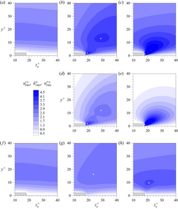
Figure 6 shows the contour plots of the root-mean-square (r.m.s.) values of the streamwise velocity fluctuations. Profiles in the top, middle and bottom rows refer to the total, periodic and turbulent fluctuations, respectively, as defined in (2.9). In figures 6(a,b,c) for the total fluctuations, two local peaks occur for  $\beta = 0^{\circ }$, the most energetic one located in the proximity of the slot. Only one local peak is computed for
 $\beta = 75^{\circ }$, at the slot. The positions of these local peaks are the same as those of the periodic fluctuations caused by the SJS, shown in figures 6(d,e). The periodic fluctuations are most intense for
 $\beta = 75^{\circ }$ because part of the SJS velocity component is aligned along the streamwise direction. The periodic forcing becomes weaker at locations further away from the SJS slots because the streamwise velocity fluctuates the most near the SJS slots, causing only one local peak. For
 $\beta = 0^{\circ }$, the streamwise velocity of SJS is zero at the SJS slots, so no additional streamwise velocity fluctuations is found. During the blowing phase, a large near-wall velocity against the main channel flow is generated near the slot exit. However, during the suction phase near the slot exit, the streamwise velocity component is enhanced near the wall. These opposite behaviours lead to the local peak of the fluctuation that is closer to the slot. The other peak is induced by the blowing SJS only because the influenced region by the blowing SJS is larger than that by the suctioning SJS. As the locations of influence of blowing and suctioning are different, the fluid motions lead to two local peaks of the periodic fluctuations. Moreover, it is evident that the lift-up effect of the SJS occurs as soon as they discharge from the orifices. The periodic fluctuations are more energetic than the turbulent fluctuations, although the latter grow with respect to the uncontrolled case, as depicted in figures 6(g,h).
Contours of root-mean-square values of the streamwise velocity fluctuations,  $u'^+_{rms}$,
 $\tilde {u}^+_{rms}$ and
 $u''^+_{rms}$, in the
 $y$–
 $z$ view. The local peak positions are denoted by the white crosses. The panels show: (a) SJS off,
 $u'^+_{rms}$; (b)
 $\beta = 0^{\circ }$,
 $u'^+_{rms}$; (c)
 $\beta = 75^{\circ }$,
 $u'^+_{rms}$; (d)
 $\beta = 0^{\circ }$,
 $\tilde {u}^+_{rms}$; (e)
 $\beta = 75^{\circ }$,
 $\tilde {u}^+_{rms}$; ( f) SJS off,
 $u''^+_{rms}$; (g)
 $\beta = 0^{\circ }$,
 $u''^+_{rms}$; (h)
 $\beta = 75^{\circ }$,
 $u''^+_{rms}$.

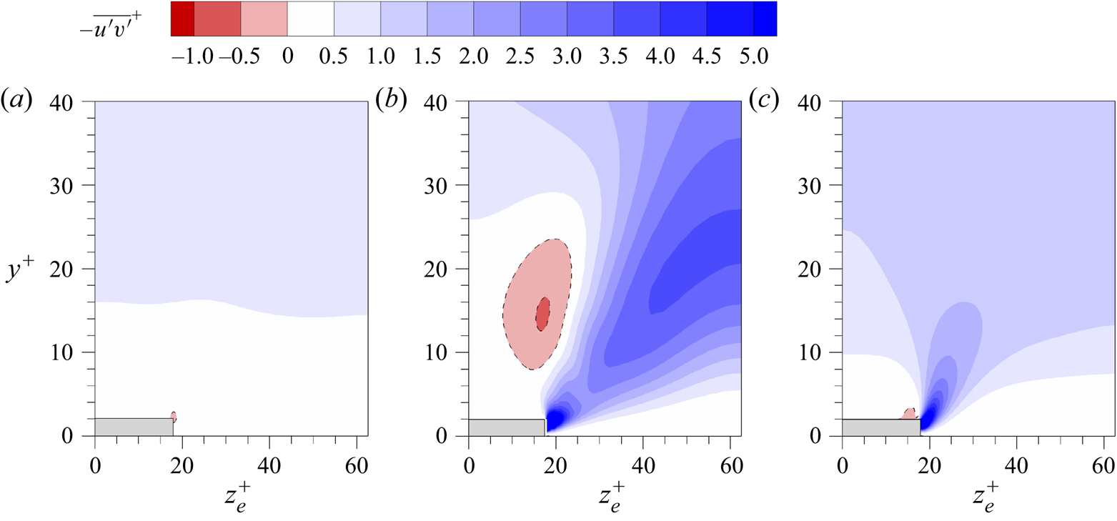
Figure 7 shows that the Reynolds shear stresses  $-\overline {u'v'}^+$, given by the total fluctuations, are increased by the SJS. In both controlled cases,
 $\beta = 0^{\circ }$ and
 $75^{\circ }$, larger Reynolds stress values than with the SJS off occur near the slots. The Reynolds stress values in the SJS cases are comparable near the slot, but for
 $\beta = 0^{\circ }$, large values are found above
 $y^+=15$ between the slots. The case for
 $\beta = 0^{\circ }$ also presents a region of Reynolds stress of opposite sign, centred at
 $y^+$=12 from the edge of the step wall. In the region where the Reynolds stress values are negative, the time and spatially averaged flow moves down towards the steps, as shown in figure 4. The low-speed region of streamwise velocity is generated by the blowing SJS and gives a negative
 $u'$, while when this part of flow is accelerated upwards, which has a positive
 $v'$, a region with negative
 $\overline {u'v'}$ is created. In the region where
 $\overline {u'v'}$ is positive, the flow motion in the wall-normal direction is opposite to that in the region of negative sign, although the flow motion is also in the streamwise direction.


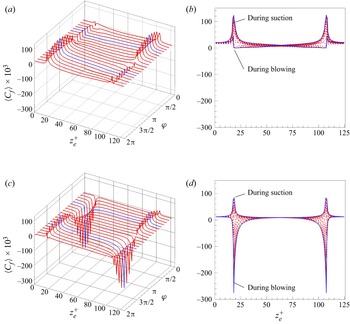
The phase and spatially ensemble averaged skin-friction coefficients are influenced significantly by the SJS, as shown in figure 8. Fluid is blown out from the left slot and is drawn in at the right slot from  $\varphi = 0$ to
 $\varphi = {\rm \pi}$, while the opposite occurs in the other half-period. In both cases,
 $\beta = 0 ^{\circ }$ and
 $\beta = 75^{\circ }$, and near the slots, the wall-friction drag is reduced during blowing and increased during suction. The drag is never negative for
 $\beta = 0 ^{\circ }$, while it is decreased significantly and becomes negative for
 $\beta = 75 ^{\circ }$. The integral of the reduced drag offsets the integral of the raised drag for
 $\beta = 75 ^{\circ }$, so an overall drag reduction is obtained.
Distributions of the phase and spatially ensemble averaged skin-friction coefficient. The blue lines denote the profiles at phases  $\varphi ={\rm \pi} / 2$ and
 $3 {\rm \pi}/2$. (a) Three-dimensional,
 $\beta = 0 ^{\circ }$; (b) two-dimensional,
 $\beta = 0 ^{\circ }$; (c) three-dimensional,
 $\beta = 75 ^{\circ }$; (d) two-dimensional,
 $\beta = 75 ^{\circ }$.

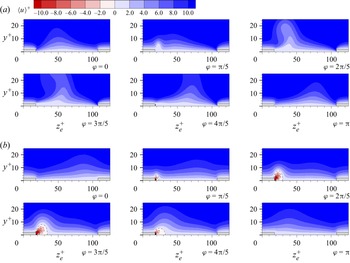
The phase and spatially ensemble averaged streamwise velocity  $\langle u \rangle ^+$ in the near-wall region is shown in figure 9 for half the period. The blowing from the left slot influences the streamwise velocity to larger wall-normal distances than the suction from the right slot. Fluid with small streamwise velocity is blown upwards by the left SJS, while fluid with large streamwise velocity is brought downwards by the right SJS. The former reduces drag, while the latter increases it. The SJS blowing with
 $\beta = 0^{\circ }$ influence the flow to larger wall-normal locations than the SJS blowing with
 $\beta = 75^{\circ }$. The counter flow is generated by the SJS with
 $\beta = 75^{\circ }$ during blowing, as depicted at
 $\varphi = 3{\rm \pi} /5$.
Contours of phase and spatially averaged streamwise velocities  $\langle u \rangle ^+$ in the
 $y$–
 $z$ plane at different phases for the cases (a)
 $\beta = 0^{\circ }$, (b)
 $\beta = 75^{\circ }$.

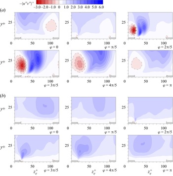
Figure 10 shows the contour plots of the Reynolds shear stresses  $-\langle u''v'' \rangle ^+$ given by the purely turbulent fluctuations for
 $\beta = 0^{\circ }$ and
 $\beta = 75^{\circ }$ from
 $\varphi = 0$ to
 $\varphi = {\rm \pi}$. The Reynolds shear stresses are enhanced by blowing, while the drag is decreased. Both positive and negative values of
 $-\langle u''v'' \rangle ^+$ are produced by the blowing region of the SJS for
 $\beta = 0^{\circ }$. The region with negative values of
 $-\langle u''v'' \rangle ^+$ is closer to the steps than the region with positive values. For
 $\beta = 75^{\circ }$, the positive values of
 $-\langle u''v'' \rangle ^+$ dominate the flow field, while the region with negative values is negligible. As shown by the contours of
 $\overline {u'v'}^+$ and
 $\langle u''v'' \rangle ^+$ in figures 7 and 10, large values of
 $\overline {u'v'}^+$ occur near the slots, while the values of
 $\langle u''v'' \rangle ^+$ are low, indicating that the periodic velocity fluctuations contribute the most to the total Reynolds shear stress there.
Contours of the Reynolds shear stress  $-\langle u''v'' \rangle ^+$ in the
 $y$–
 $z$ plane at different phases for the cases (a)
 $\beta = 0 ^{\circ }$, (b)
 $\beta = 75 ^{\circ }$.

The overall picture is therefore that the SJS cause drag reduction for  $\beta = 75^{\circ }$ through the intense near-wall counter flow being larger than the forward flow occurring in the near-wall region in the proximity of the SJS slots, despite the intensified Reynolds shear stresses. The drag-increasing case for
 $\beta = 0^{\circ }$ also enhances the Reynolds shear stresses, but it does not benefit from the counter flow because the SJS are aligned along the spanwise direction only.
3.3. Turbulent-flow structures
Instantaneous flows for the cases with  $\beta = 0^{\circ }$ and
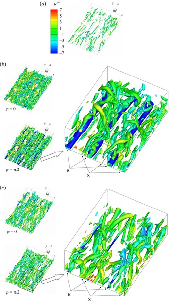
 $75^{\circ }$ are discussed in this subsection. Figure 11 shows the isosurfaces of
 $\lambda _2^+ = -2$ in the bottom half-channel at different phases. The
 $\lambda _2$ technique to detect the vortex cores was developed by Jeong & Hussain (Reference Jeong and Hussain1995). The flows altered by the SJS display more intense vortical structures than the case without SJS forcing, irrespective of whether the drag reduces or increases. The response of the flow to the forcing is therefore different from other spanwise forcing methods, such as streamwise-travelling waves of spanwise wall velocity (Quadrio et al. Reference Quadrio, Ricco and Viotti2009; Quadrio & Ricco Reference Quadrio and Ricco2011), which lead to a less intense and more sporadic population of near-wall vortical structures accompanied by a reduction of wall-friction drag. Vortical structures, shaped like elongated tubes near the SJS slots, are generated during blowing, at the phase
 $\varphi = {\rm \pi}/2$. At the phase
 $\varphi = 0$ and during suction, the vortical structures are broken by the main flow and the vortices are more apart than when
 $\varphi = {\rm \pi}/2$. Figure 11 shows that the diameter and the intensity of the weaker vortices, coloured in green and located in the bulk of the flow, are only slightly influenced by the SJS angle. In the
 $\beta =0^\circ$ case, intense elongated tubular structures appear near the wall and in the proximity of the SJS exits where blowing occurs. These structures are much weaker in the
 $\beta =75^\circ$ case.
Isosurfaces of  $\lambda _2^+ = -2$ at different phases for the cases with (a) SJS off, (b)
 $\beta = 0^{\circ }$, and (c)
 $\beta = 75^{\circ }$. The isosurfaces are coloured by
 $u'^+$, and ‘B’ and ‘S’ stand for blowing and suctioning slots, respectively.

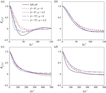
Two-point autocorrelations, defined as
 \begin{equation} R_{u''u''}(\Delta x_i) = \frac{\overline{u''(x_i+\Delta x_i)\,u''(x_i)}}{\overline{u''u''}}, \end{equation}
are computed for  $x_i=x,z$. Figure 12 shows the distributions of
 $R_{u''u''}(\Delta x)$ and
 $R_{u''u''}(\Delta z)$ at different heights for cases with SJS off,
 $\beta = 0 ^{\circ }$ and
 $\beta = 75 ^{\circ }$. Figure 12(a) shows that at
 $y^+=10$, for
 $\beta = 75 ^{\circ }$, the spanwise turbulent length scales are smallest, while for
 $\beta = 0 ^{\circ }$, the scales are largest, confirming quantitatively what is observed in the flow visualizations of figure 11. In figure 12(b), the
 $R_{u''u''}(\Delta z^+)$ values at higher locations (
 $y^+=100$) are similar for both SJS cases, as also shown by the green vortices in figure 11. Figure 12(c) shows that at
 $y^+=10$, the streamwise turbulent length scales are reduced slightly by SJS, and the case
 $\beta = 0 ^{\circ }$ shows the shortest scales when the SJS velocity amplitude reaches its maximum. Figure 12(d) shows that at
 $y^+=100$, the SJS increase the length scales the most when
 $\beta = 75 ^{\circ }$. The SJS influence the spanwise length scales more than the streamwise length scales.
Spanwise and streamwise two-point correlations of streamwise velocity fluctuations  $u''$, for: (a)
 $y^+ = 10$; (b)
 $y^+ = 100$; (c)
 $y^+ = 10$; (d)
 $y^+ = 100$.

3.4. Flow and power balance of the jet-sheet actuator
A model of the actuators that generate the SJS is presented in this subsection. The focus is on the flow inside the actuators, located underneath the channel walls, and on the power required to operate the SJS. As for the turbulent channel flow simulations, the channel half-height  $h^*$ and the centreline velocity
 $U^*_p$ of the laminar parabolic Poiseuille flow of the reference smooth channel case are used for scaling.
3.4.1. Flow in the cavity chambers
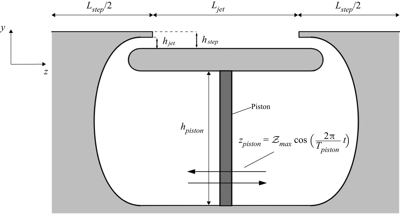
Figure 13 shows a schematic of the system. A piston separates two chambers of a cavity and oscillates sinusoidally along the spanwise direction, forcing the fluid in the compression chamber to discharge through the SJS opening and out into the channel. Simultaneously, the pressure drops in the suction chamber, causing the fluid to enter the SJS opening and to fill the chamber. The flows in the chambers alternate their behaviour every half-cycle, according to the motion of the piston. The parameters of the chambers and the simulation details are listed in table 2.
Schematic of the cavity chambers. The thickness of the piston is not to scale.

Simulation and chamber parameters, where  $\langle w\rangle _{{jet,max}}$ is the spatially averaged SJS velocity, and
 $\Delta t$ is the time step. The other quantities are defined in figure 13.

The in-house code SHEFFlow is used to compute the flow in the chambers and outside the SJS openings. The domain of the simulation consists of the chambers and half of the channel above them. The flow is assumed to be two-dimensional. Mirror boundary conditions are imposed at the half-channel boundary, and periodic boundary conditions are enforced at the sides of the computational domain. Figure 13 represents the purely spanwise case ( $\beta =0 ^{\circ }$). In the case of oblique SJS, the exits would require inclined vanes to drive the fluid out into the channel at an angle. The losses due to the three-dimensionality of the vanes are assumed small with respect to the rest of the losses, an approximation that is confirmed in § 3.4.4. The wall that separates the SJS and the channel has a finite thickness, which is smaller than the height of the exits. This finite thickness avoids a sharp wall end at the exit, which would create intense velocity gradients when the fluid leaves the chamber.
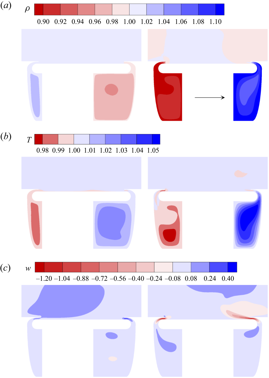
Figure 14 shows that the density and the temperature are not uniform inside the chambers. When the piston is in the neutral position ( $\varphi = {\rm \pi}/2$), the piston velocity is maximum. The fluid is then compressed in the right chamber, while in the left chamber the fluid expands. At
 $\varphi = 0$, the displacement is maximum and the density in the right chamber decreases by releasing the fluid inside the chamber to the channel, while in the left chamber, the fluid enters the chamber and the density increases. These compressibility effects cause a phase lag of about
 $\varphi =0.03{\rm \pi}$ between the pressure experienced by the piston and the velocity of the piston, rendering the power spent lower than that without delay.
Contours of (a) density, (b) temperature, and (c) spanwise velocity, at phases  $\varphi = 0$ (left) and
 $\varphi = {\rm \pi}/2$ (right). The horizontal arrow indicates the direction of piston motion.

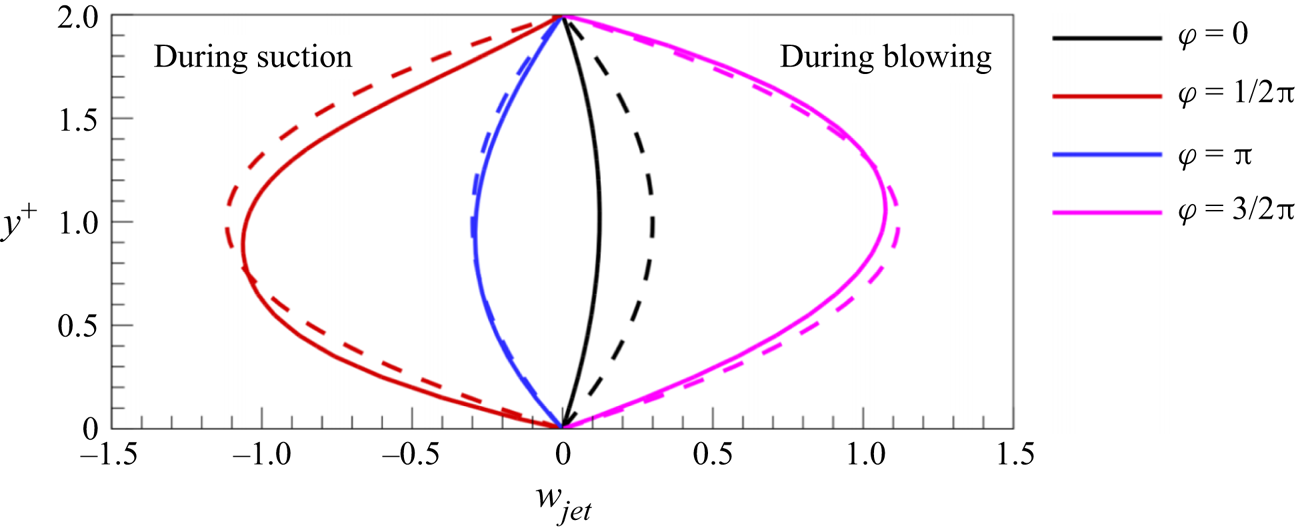
Figure 15 shows that the computed horizontal SJS velocity profiles are approximated well by parabolic profiles. The results of the two-dimensional simulation therefore validate the assumption of a parabolic SJS flow for the three-dimensional channel flow simulation, modelled by (2.4). The largest deviations from a symmetric profile occur when the mass flow rate is maximum during blowing or suction. When air exits a chamber and enters the channel, the peak of the maximum velocity is slightly larger than in the mid position at  $y^+=1$, while the contrary happens in the suction phase, during which the maximum velocity peak is lower than in the mid position. In the blowing phase, this small effect is caused by a localized region of low pressure at the tip of the step wall. This low pressure causes the air exiting the SJS aperture to move upwards, away from the jet wall. In the suction phase, the curvature of the chamber forces the air in the lower half of the SJS aperture to turn downwards.
Velocity profiles at the exit of the left cavity at different phases of the oscillation. The dashed lines represent the parabolic boundary condition given in (2.4), imposed in the three-dimensional channel flow simulations. The solid lines represent the velocity profiles obtained with the two-dimensional simulation.

3.4.2. Motion of the piston
The position of the piston is described by
 \begin{equation} z_{{piston}} = \mathcal{Z}_{{max}} \cos \left(\frac{2{\rm \pi}}{T_{{piston}}}\,t\right),\end{equation}
where  $T_{{piston}}$ is the period of oscillation of the piston, and
 $\mathcal {Z}_{{max}}$ is the maximum displacement travelled by the piston with respect to the central position. The period of oscillation
 $T_{{piston}}$ is the same as the period of oscillation
 $T_{{osc}}$ of the SJS boundary condition in the full three-dimensional simulation.
As the flow inside the chambers is compressible, an exact a priori relationship between the piston motion and the SJS velocity cannot be found without simulating the flow because the fluid density at the piston surfaces and the fluid density at the cavity exits are not known. Therefore, in order to obtain an estimate of the maximum displacement  $\mathcal {Z}_{{max}}$ as a function of the average SJS velocity, the incompressible mass conservation equation is used:
 \begin{equation} \int_A \boldsymbol{u} \boldsymbol{\cdot} \boldsymbol{n}\,\mathrm{d} A = 0, \end{equation}
where  $A$ is the surface of the chamber including the SJS orifices, and
 $\boldsymbol {n}$ is the normal unit vector perpendicular to
 $A$, pointing outwards. Since the vectors
 $\boldsymbol {n}$ for the piston surface and for the SJS exit surface point in the spanwise direction, (3.3) becomes
 \begin{equation} {-}w_{{piston}} (t)\,A_{{piston}}+ \int_{A_{{fluid}}} w_{{jet}} (y,t)\,\mathrm{d} A_{fluid} = 0, \end{equation}
where  $w_{{piston}}$ is the velocity of the piston,
 $w_{{jet}}$ is the velocity profile at the SJS exit,
 $A_{{piston}}$ is the surface of the piston, and
 $A_{\mathrm {fluid}}$ is the area of the SJS apertures. Writing (3.4) per unit depth, the surface integral becomes
 \begin{equation} {-}w_{{piston}} (t)\,h_{{piston}} + \int_0^{h_{{jet}}} w_{{jet}} (y,t)\, \mathrm{d}y = 0, \end{equation}
where  $h_{{piston}}$ is the height of the piston. The spatial mean velocity of the SJS, defined as
 \begin{equation} \langle w\rangle_{{jet}}(t)=\frac{1}{h_{{jet}}} \int_{h_{{jet}}} w_{{jet}} (y,t)\, \mathrm{d}y, \end{equation}
and  $w_{{piston}}$, found from differentiating (3.2), are substituted into (3.5) to find the maximum displacement of the piston:
 \begin{equation} \mathcal{Z}_{{max}} = \frac{T_{piston}}{2{\rm \pi}}\,\frac{h_{{jet}}}{h_{{piston}}}\, \langle W\rangle_{{jet,max}},\end{equation}
where  $\langle W\rangle _{{jet,max}}$ is the maximum spatial mean velocity of the SJS within a period. The boundary conditions for the SJS velocity in the three-dimensional simulation with the parameters given in table 2 result in amplitude
 $\mathcal {Z}_{{max}}=0.079$ and maximum piston velocity
 $W_{{piston,max}}= 0.031$.
3.4.3. Power balance of the cavity flow for  $\beta =0^\circ$

The first step to study the power balance of the SJS actuators is to calculate the power per unit depth required to move the piston,  $\mathcal {W}_{{piston}}$, in the two-dimensional configuration (
 $\beta =0^\circ$). This power is exerted by the force that the piston has to overcome at any time to generate the SJS, given by the difference of the integrated pressures on the two sides of the piston as a function of time. The power
 $\mathcal {W}_{{piston}}$ is
 \begin{equation} \mathcal{W}_{{piston}}(t) = w_{{piston}}(t)\int_{h_{{piston}}} \Delta p_{{piston}}(y,t)\,\mathrm{d}y, \end{equation}
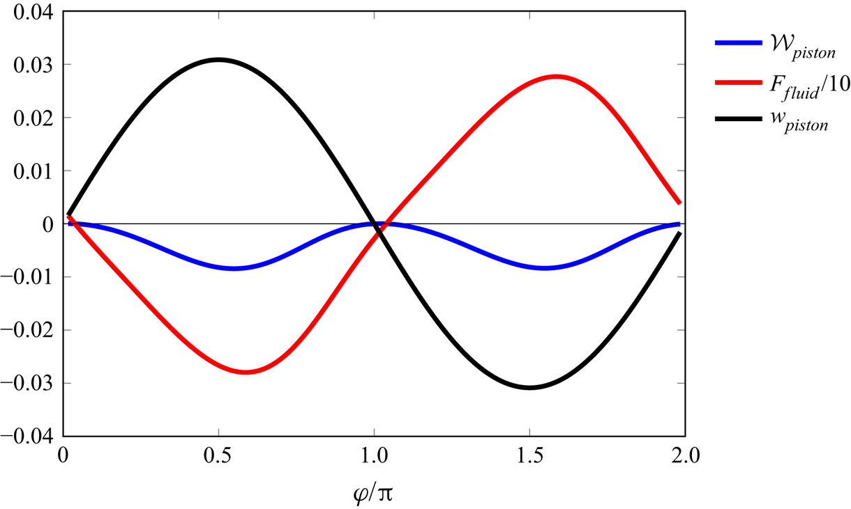
where  $\Delta p_{{piston}}$ is the difference between the pressures on the two sides of the piston. Figure 16 shows the piston velocity
 $w_{{piston}}(t)$, the force per unit depth of the cavity acting on the piston,
 \begin{equation} F_{{piston}} (t) = \int_{h_{{piston}}} \Delta p_{{piston}} (y,t)\,\mathrm{d}y, \end{equation}
and the power  $\mathcal {W}_{{piston}}$ during a period of oscillation. A phase lag of about
 $\varphi =0.1{\rm \pi}$, shown in figure 16, occurs between the integrated pressure
 $\Delta F_{{piston}}$ experienced by the piston and the velocity of the piston
 $w_{{piston}}(t)$. This phase lag causes the power spent to be lower than that if the maxima of the piston force and the piston velocity occurred at the same time. For the parameters given in table 2, the average power required to move the piston is
 $\overline {\mathcal {W}}_{{piston}}=8\times 10^{-3}$.
Ensemble average of the velocity of the piston, pressure difference, and power required to move the piston.

The power balance inside the cavity chambers is studied through the balance equation for the total power integrated over the control volume. The balance equation, derived in Appendix C following Panton (Reference Panton2013), reads
 \begin{align} & \underbrace{\frac{\mathrm{d}}{\mathrm{d} t} \int_V \rho \left(e + \frac{\vert \boldsymbol{u} \vert^2}{2} \right) \mathrm{d}V }_{\mathrm{d}\mathcal{E}/\mathrm{d}t}={-} \underbrace{\int_{A_{fluid}} p \boldsymbol{u} \boldsymbol{\cdot} \boldsymbol{n}\,\mathrm{d}A}_{\mathcal{P}_{fluid}} -\underbrace{\int_{A_{fluid}} \rho e \boldsymbol{u} \boldsymbol{\cdot} \boldsymbol{n}\,\mathrm{d}A}_{\mathcal{F}_{i-fluid}} \nonumber\\ &\quad -\underbrace{\int_{A_{fluid}} \rho\, \frac{\vert \boldsymbol{u} \vert^2}{2}\,\boldsymbol{u} \boldsymbol{\cdot} \boldsymbol{n}\,\mathrm{d}A}_{\mathcal{F}_{m-fluid}} -\underbrace{w_{{piston}}(t)\int_{A_{piston}} \Delta p_{{piston}}\,\mathrm{d}A}_{\mathcal{W}_{{piston}}} + \underbrace{\frac{1}{Re_p}\int_{A_{fluid}} (\boldsymbol{\underline{\tau}} \boldsymbol{\cdot} \boldsymbol{u}) \boldsymbol{\cdot} \boldsymbol{n}\,\mathrm{d}A}_{\mathcal{T}_{fluid}} \nonumber\\ &\quad +\underbrace{\frac{1}{Re_p} \int_A k\,\boldsymbol{\nabla} T \boldsymbol{\cdot} \boldsymbol{n}\,\mathrm{d}A}_{\mathcal{Q}}. \end{align}
Equation (3.10) expresses the following physical mechanisms. The power injected into the cavity chambers via the pressure work of the piston  $\mathcal {W}_{{piston}}$ partly generates the time rate of change of the integrated total energy,
 $\mathrm {d}\mathcal {E}/\mathrm {d}t$, is partly transferred to the channel as the fluid exhausts through the SJS apertures, via the flux of internal energy per unit time
 $\mathcal {F}_{i-fluid}$, the mechanical power flux
 $\mathcal {F}_{m-fluid}$, the pressure work
 $\mathcal {P}_{fluid}$ and the shear stress work
 $\mathcal {T}_{fluid}$ of the SJS, and is lost to the outside of the cavity chambers via the heat transfer
 $\mathcal {Q}$.
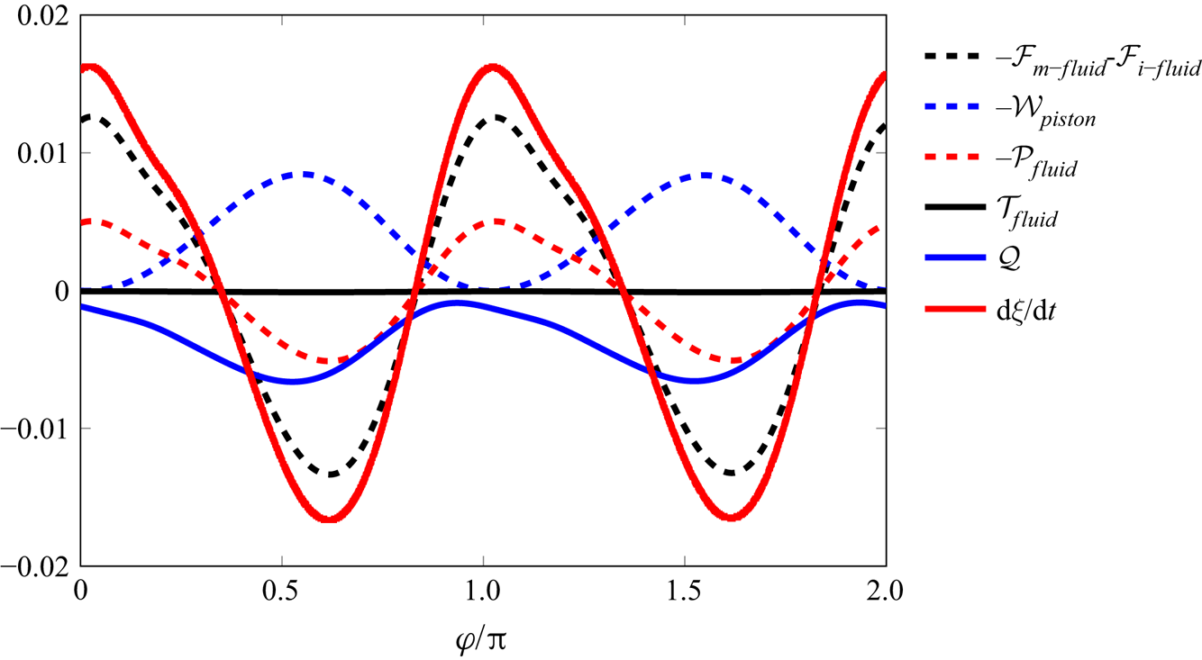
Figure 17 shows the time evolution of the terms of (3.10) during one period of oscillation. The kinetic energy term  $\mathrm {d}\mathcal {E}/\mathrm {d}t$ shows the most intense oscillations, while the power transferred via the shear stresses at the SJS apertures,
 $\mathcal {T}_{fluid}$, is found to be negligible. At any phase of the oscillation, the piston always injects power into the chambers, while heat is always extracted from the chambers. The flux terms and the pressure term related to the SJS instead oscillate between positive and negative values, being directly related to the SJS.
Time evolution of terms in the power equation (3.10). Positive values indicate power into the chambers, while negative values indicate power lost from the chambers.

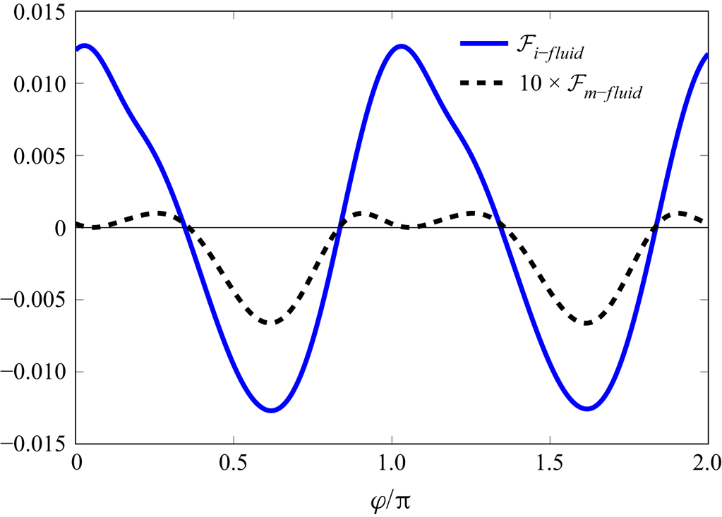
Figure 18 displays the time evolution of the flux terms  $\mathcal {F}_{m-fluid}$ and
 $\mathcal {F}_{i-fluid}$. The flux of internal energy per unit time
 $\mathcal {F}_{i-fluid}$ is much larger than the mechanical power flux
 $\mathcal {F}_{m-fluid}$ because the difference in temperature at the SJS exits is larger than the difference in the averaged velocities. Mechanical power is passed from the chambers to the channel for
 $47\,\%$ of an oscillating period, during
 $(0.31 {\rm \pi}, 0.86 {\rm \pi})$ and
 $(1.31 {\rm \pi}, 1.86 {\rm \pi})$. The time-averaged values of the fluxes of mechanical power and internal energy per unit time are
 $3.04 \times 10^{-4}$ and
 $1.84 \times 10^{-4}$, i.e. the mechanical part takes
 $62.3\,\%$ of the convective flux and is
 $3.8\,\%$ of the time average of
 $\mathcal {W}_{{piston}}$.
Time evolution of mechanical power flux  $\mathcal {F}_{m-fluid}$ and the flux of internal energy per unit time
 $\mathcal {F}_{i-fluid}$.

The terms in (3.10) are time-averaged to quantify further the balance of the SJS actuator. The averaged values are listed in table 3. For the convective flux and the pressure work, power flows into the two chambers when the value is negative and out of them when the value is positive. The channel flow thus receives power from the SJS in the three ways, i.e. through the flux of internal energy per unit time  $\overline {\mathcal {F}}_{i-fluid}$, the mechanical power flux
 $\overline {\mathcal {F}}_{m-fluid}$, and the pressure work term
 $\overline {\mathcal {P}}_{fluid}$. The last two types of power are relevant for flow control:
 $\overline {\mathcal {F}}_{m-fluid}$ and
 $\overline {\mathcal {P}}_{fluid}$ are
 $3.8\,\%$ and
 $1.7\,\%$ of
 $\overline {\mathcal {W}}_{{piston}}$, respectively. The effective power
 $\overline {\mathcal {P}}_{\mathrm {jet-sheet}}$ is
 \begin{equation} \overline{\mathcal{P}}_{{jet-sheet}} = \overline{\mathcal{F}}_{m-fluid} + \overline{\mathcal{P}}_{fluid}= 0.038 \times \overline{\mathcal{W}}_{{piston}} + 0.017 \times \overline{\mathcal{W}}_{{piston}}=0.054 \times \overline{\mathcal{W}}_{piston}. \end{equation}
The efficiency of the SJS actuator is therefore  $\overline {\mathcal {P}}_{{jet-sheet}}/\overline {\mathcal {W}}_{{piston}}=5.4\,\%$. A more conservative estimation of the power employed by distributed suction and blowing was utilized by Bewley, Moin & Temam (Reference Bewley, Moin and Temam2001), Chung & Talha (Reference Chung and Talha2011) and Stroh et al. (Reference Stroh, Frohnapfel, Schlatter and Hasegawa2015). They used the absolute values of the integrands that define
 $\overline {\mathcal {F}}_{m-fluid}$ and
 $\overline {\mathcal {P}}_{fluid}$, as defined in (3.12) and (3.13) below. If we adopt those authors’ definitions of power consumption,
 $$\begin{gather} \lvert \overline{\mathcal{F}}_{m-fluid} \rvert =\int_{T_{osc}} \int_{A_{fluid}} \left\lvert \rho\,\frac{\vert \boldsymbol{u} \vert^2}{2}\,\boldsymbol{u} \boldsymbol{\cdot}\boldsymbol{n} \right\rvert\mathrm{d}A\,\mathrm{d}t, \end{gather}$$
 $$\begin{gather}\lvert \overline{\mathcal{P}}_{fluid} \rvert = \int_{T_{osc}} \int_{A_{fluid}} \lvert p \boldsymbol{u} \boldsymbol{\cdot} \boldsymbol{n} \rvert\,\mathrm{d}A\, \mathrm{d}t, \end{gather}$$
then we find  $\lvert \overline {\mathcal {F}}_{m-fluid} \rvert =0.42 \times 10^{-3} = 0.052 \times \overline {\mathcal {W}}_{{piston}}$ and
 $\lvert \overline {\mathcal {P}}_{fluid} \rvert =6.22 \times 10^{-3} = 0.774 \times \overline {\mathcal {W}}_{{piston}}$.
Time-averaged terms in (3.10).

3.4.4. Power balance of the cavity flow for $\beta \neq 0^\circ$

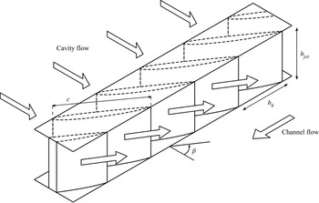
The analysis of the power efficiency of the cavity flow presented in § 3.4.3 is limited to the two-dimensional case with injection angle  $\beta =0^\circ$. To compute the power efficiency of the cavity flow for finite angles
 $\beta$, we estimate the power loss by considering the flow through a series of guide vanes placed between the cavity and the SJS exits, as shown in figure 19. For the power-loss estimation, it is useful to refer to studies on flows through guide vanes in low-speed wind tunnels. The Reynolds number
 $\mbox {{Re}}_c$ used in the analysis of guide vanes is typically based on the mean inlet velocity and the chord of the guide vanes; in our case, a sound estimate based on the maximum inlet velocity is
 $\mbox {{Re}}_c=25\,000$. According to Sahlin & Johansson (Reference Sahlin and Johansson1991) and Lindgren, Österlund & Johansson (Reference Lindgren, Österlund and Johansson1998), the guide-vane pressure-loss coefficient
 $\mathcal {K}$ at this chord Reynolds number for a
 $90^{\circ }$ turn and expansion ratios close to unity varies in the range
 \begin{equation} \mathcal{K} = \frac{\Delta H^*}{q^*_{{in}}}=0.08-0.12, \end{equation}
where  $\Delta H^* = (p^*_{{in}}+q^*_{{in}})- (p^*_{{out}}+q^*_{{out}})$; the subscripts ‘in’ and ‘out’ stand for the flow entering and exhausting from the vane, respectively, and
 $q^*_{{in}}=\rho _c^*\, \langle W\rangle _{{jet,max}}^{*2}/2=q^*_{{out}}$ because the expansion ratio is assumed to be unity. A
 $90^{\circ }$ turning vane represents the worst possible scenario for the power loss, and adequately models the SJS case with
 $\beta =75^{\circ }$, which leads to the maximum drag reduction. The estimate of the pressure coefficient translates to a 10 % decrease of the mechanical power flux
 $\overline {\mathcal {F}}_{m-fluid}$ injected into the channel. The overall efficiency of the device reduces to 5.2 %. Moreover, it means that the case with
 $\beta =75^{\circ }$ needs
 $1.11 \times \overline {\mathcal {W}}_{{piston}}$ to have the same amount of power at the SJS exits as the case with
 $\beta =0^{\circ }$.
Schematic of the guide vanes used to change the direction of the flow to angle  $\beta$.

It is also instructive to compare the power used to activate the piston with the power saved by drag reduction. From (2.13), the power spent per streamwise length used to drive the fluid in the channel is
 \begin{equation} \overline{\mathcal{P}}_{{channel}}^*=2\tau_w^*U_b^* (L^*_{jet} + L^*_{step})= [C_f] \rho_c^* U_b^{*3}(L^*_{jet} + L^*_{step}). \end{equation}
Using the channel half-height  $h^*$ and the centreline velocity
 $U_p^*$ for scaling, one finds
 \begin{equation} \overline{\mathcal{P}}_{{channel}}=[C_f] \left( \frac{U_b^*}{U_p^*} \right)^3 \frac{L^*_{jet} + L^*_{step}}{h^*}=16.97 \times 10^{{-}4}. \end{equation}
For  $\beta = 75^{\circ }$, the skin-friction coefficient is reduced by 10.5 %, which leads to the maximum power saved by the SJS actuation,
 $\overline {\mathcal {P}}_{{channel,SJSoff}} - \overline {\mathcal {P}}_{{channel,SJS75}}= 17.82 \times 10^{-5}$. The net power saved in this case is
 $\overline {\mathcal {P}}_{{channel,SJSoff}} - \overline {\mathcal {P}}_{{channel, SJS75}} - 1.11 \times \overline {\mathcal {W}}_{{piston}}= -8.75 \times 10^{-3}$, which means that the actuation power is larger than the saved power due to drag reduction.
4. Conclusions
Skin-friction drag reduction generated by wall-tangential synthetic jet sheets in a turbulent channel flow at  $\mbox {{Re}}_\tau = 180$ has been investigated by direct numerical simulations. The jet sheets eject from slots located below steps that are aligned along the streamwise direction. The effect of the jet-sheet angle with respect to the streamwise direction has been studied. Compared to the smooth channel flow, the friction drag decreases by
 $10.5\,\%$ and increases by
 $98.4\,\%$ for thin jet heights
 $h_{{jet}}^+=2$ and jet-sheet angles
 $75 ^{\circ }$ and
 $0 ^{\circ }$, respectively. Drag-reduction margins as large as
 $30\,\%$ are obtained for jet sheets exhausting from thicker slots and for distances between slots smaller than the spanwise length scale of the low-speed streaks. The drag reduction on the jet walls offsets the drag increase on the step walls for jet-sheet angle
 $\beta = 75 ^{\circ }$. The spatially averaged skin-friction coefficients fluctuate in time with a period that is half of the jet-sheet period.
In all the cases, there occurs an intense variation of the wall-shear stress along the spanwise direction. The phase-averaged results indicate that blowing decreases the drag, and suction increases it. When the jet sheets eject at a large angle, the time and spatially averaged results show that the friction drag decreases significantly near the slots. Although the jet sheets are synthetic and therefore their net mass flow rate is null, the global friction drag reduction is caused by a net negative wall-shear stress near the jet-sheet openings, which is due to the nonlinear interaction between the jet sheets and the streamwise mean flow.
The velocity fluctuations and the Reynolds stresses in the controlled cases are larger than those for the cases with jet sheets off. The total fluctuations are enhanced because the jet sheets add periodic perturbation into the flow and because the purely turbulent fluctuations are also enhanced. The growth of velocity fluctuations causes the total and purely turbulent Reynolds shear stresses to increase with respect to the reference case when the jet sheets are on, even when drag reduction occurs. Instantaneous flow visualizations also show that eddies are more intense when the flow is forced by the jet sheets. Low-speed and high-speed regions are elongated by the jet sheets when the jet-sheet velocity increases. For  $\beta = 0 ^{\circ }$, the vortices are closer to the channel centre than for
 $\beta = 75 ^{\circ }$. For
 $\beta = 0 ^{\circ }$, the spanwise length scales of the vortices are wider than those for
 $\beta = 75 ^{\circ }$, as shown by two-point autocorrelations.
A power balance analysis has also been carried out for the actuator by simulating the flow inside a cavity where a piston creates the air motion that generates the jet sheets. As air is compressed or expanded cyclically inside the chambers, the power input by the piston is transferred to the jet sheets, but also transformed into internal energy per unit time and lost via heat transfer instead of being used as kinetic energy of the jet sheets. During part of the cycle, the compressed air expands, transforming internal energy into kinetic energy. For the tested configurations, the power spent to generate the jet sheets is larger than that saved thanks to the reduction of wall friction. It would be interesting to test the actuator with a fluid that does not experience the compressibility effects of air, like water, in order to improve the power efficiency of the actuator.
It would also be of interest to investigate the flow at larger Reynolds numbers or when driven by a constant pressure gradient. Future research should be directed to discerning how the periodic jet-sheet flow interacts with the bulk turbulent flow to generate the counter flow, a mechanism recognized to be responsible for the drag-reduction effect. In view of technological applications, it would be relevant to study the persistence of the turbulent-flow modifications downstream of a finite section of the wall surfaces where the jet sheets are enforced.
Acknowledgements
We would like to thank the referees for their valuable comments. The research work was undertaken within the framework of the H2020 EU-China project ‘DRAGY: Drag Reduction in Turbulent Boundary Layer via Flow Control’ (grant agreement ID: 690623). F.X. acknowledges financial support from the CARDC studentship for his doctoral studies. The authors acknowledge the provision of computing resources on the High Performance Computing cluster ShARC at the University of Sheffield and the Sunway TaihuLight at the National Supercomputing Center in Wuxi, China.
Declaration of interests
The authors report no conflict of interest.
Appendix A. Validation of the numerical computations
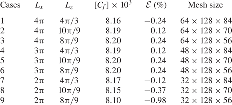
The computation of the fully developed turbulent channel flow at  $\mbox {{Re}}_\tau = 180$ is validated by several resolution checks. Table 4 shows the results of mesh independence. For case 1, the dimensions of the computational domain are
 $L_x = 4 {\rm \pi}$ and
 $L_z = 4 {\rm \pi}/3$ for the streamwise length and spanwise width, respectively. The reference mesh resolutions are
 $\Delta x^+ = 17.67$ and
 $\Delta z^+=8.98$ in the streamwise and spanwise directions, respectively, while
 $\Delta y_w^+ = 0.5$ is the distance of the first wall-normal grid point from the walls, and
 $\Delta y_c^+ = 5.56$ is the wall-normal grid spacing at the channel centre. The reference mesh has
 $128 \times 128 \times 84$ cells in the streamwise, wall-normal and spanwise directions, respectively.
Skin-friction coefficients and errors for different sizes of computational domain, using the same mesh resolution. Here,  $\Delta x^+ = 17.67$,
 $\Delta z^+=8.98$,
 $\Delta y_w^+ = 0.5$,
 $\Delta y_c^+ = 5.56$, and
 $\mathcal {E}=100 \times ([C_f] \times 10^3 - 8.18)/8.18$.

After the flow has reached its fully developed turbulent state, the skin-friction coefficient is computed to be  $[C_f]=8.16 \times 10^{-3}$ by averaging flow fields between
 $t^+ = 2187$ and
 $t^+ =4860$. This value is only
 $0.24\,\%$ different from
 $[C_f]=8.18 \times 10^{-3}$ from the DNS by Kim et al. (Reference Kim, Moin and Moser1987). The mean streamwise velocity, the root-mean-square of the velocity fluctuations, the Reynolds shear stresses, and the streamwise spectra of velocities are indistinguishable from the corresponding quantities reported by Kim et al. (Reference Kim, Moin and Moser1987), as shown in figure 20. Case
 $7$ is chosen as a compromise between a manageable computational cost and accuracy of the computation of the skin-friction coefficient. The comparisons of the mesh resolutions and the results are shown in table 5 for the smooth channel.
Comparisons of the flow quantities of Kim et al. (Reference Kim, Moin and Moser1987) and SHEFFlow. (a) Mean streamwise velocity profile. (b) Root-mean-square values of velocity fluctuations:  $u'^+_{rms}$, black solid line and squares;
 $v'^+_{rms}$, red dashed line and triangles;
 $w'^+_{rms}$, blue dot-dash line and circles. (c) Normalized viscous shear stress
 $\mu ({{\partial } \overline {u}}/{{\partial } y})/ \tau _w$, red dashed line and triangles; Reynolds shear stress
 $-\overline {u'v'}/ \tau _w$, black solid line and squares. (d) Streamwise spectra for
 $u,v,w$ at
 $y^+=30$ with:
 $E_{uu}$, black solid line and squares;
 $E_{vv}$, red dashed line and triangles;
 $E_{ww}$, blue dot-dash line and circles.

Skin-friction coefficients and errors for different mesh resolutions.

The mesh sensitivity was also studied for the controlled channel. Since the cases  $\beta = 75 ^{\circ }$ and
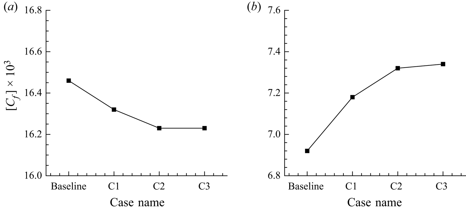
 $\beta = 0 ^{\circ }$ have large values of drag reduction and drag increase, they are chosen for the validation tests. The baseline mesh is similar to the resolution of the medium mesh. Figure 21 displays how the mesh is refined in the spanwise direction. Table 6 shows the skin-friction coefficients for different mesh resolutions. To study the mesh sensitivity, the baseline mesh is refined in three directions. Cases A, B and C are refined in the streamwise, wall-normal and spanwise directions, respectively. Comparing the results of the baseline case and case A, the differences of the skin-friction coefficients are 0.12 % and 0.43 % for
 $\beta = 0^{\circ }$ and
 $\beta = 75^{\circ }$, respectively. The differences between the baseline case and case B are 0.12 % and 0.58 % for
 $\beta = 0 ^{\circ }$ and
 $\beta = 75 ^{\circ }$, respectively. These differences are small, proving that the mesh values
 $\Delta x^+=8.84$,
 $\Delta y_w^+ = 0.2$ and
 $\Delta y_c^+ = 4.09$ are fine enough for computing the skin friction accurately. However, the results of the skin friction are very different between the baseline case and case C1, which means that the mesh resolution of the baseline case is not fine enough in the spanwise direction. As the mesh is refined in the spanwise direction, figure 22 shows a convergent trend of the skin frictions, the differences between cases C2 and C3 being negligible and 0.27 % for
 $\beta = 0^{\circ }$ and
 $\beta = 75^{\circ }$, respectively. According to these results, the mesh resolution of case C2 is therefore fine enough to resolve the flow.
Computational meshes for the study of mesh sensitivity: (a) baseline, (b) C1.

Skin-friction coefficients for the different meshes in table 6: (a)  $\beta = 0^\circ$, (b)
 $\beta = 75^\circ$.

Computational mesh resolutions and skin-friction coefficients for the study of mesh sensitivity at  $\beta = 0 ^{\circ }$ and
 $75 ^{\circ }$.

Appendix B. Dependence of drag reduction on system parameters
The effects of the SJS slot height, velocity, period of oscillation, and length of the jet wall on the drag-reduction performance are investigated. As each parameter is varied independently, the other parameters are kept the same as the optimal case studied in the main text.
B.1. Jet-sheet slot height
For the uncontrolled cases, the results show that the skin-friction coefficients are  $8.18 \times 10^{-3}$,
 $7.62 \times 10^{-3}$ and
 $7.54 \times 10^{-3}$ for
 $h^+_{jet}=2$,
 $4$ and
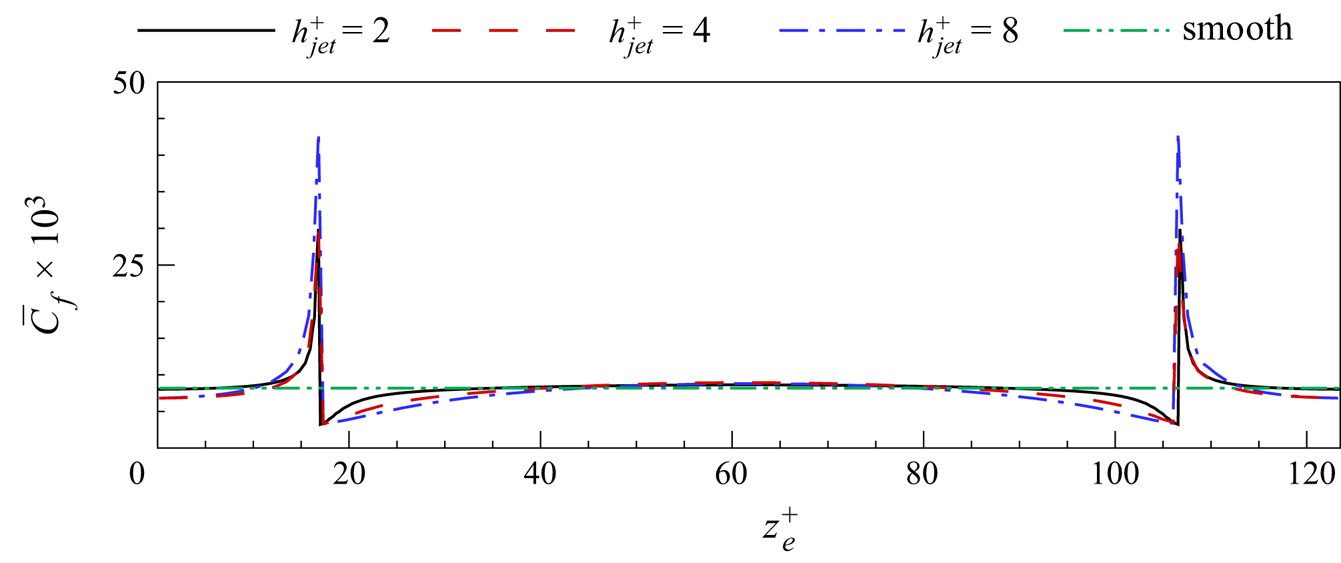
 $8$, respectively. The distributions of the time and spatially averaged skin-friction coefficients along the spanwise direction are shown in figure 23. The effect of
 $h_{{jet}}^+$ is concentrated around the step corner, reducing the drag on the jet wall and increasing the drag on the step wall. The case
 $h_{{jet}}^+ = 8$ produces the largest reduction in drag on the jet wall with respect to the smooth channel.
The time and spatially averaged skin-friction coefficients along the spanwise direction for different SJS heights for jet off cases.

The drag-reduction margins for SJS slot heights  $h^+_{jet}=2$,
 $4$,
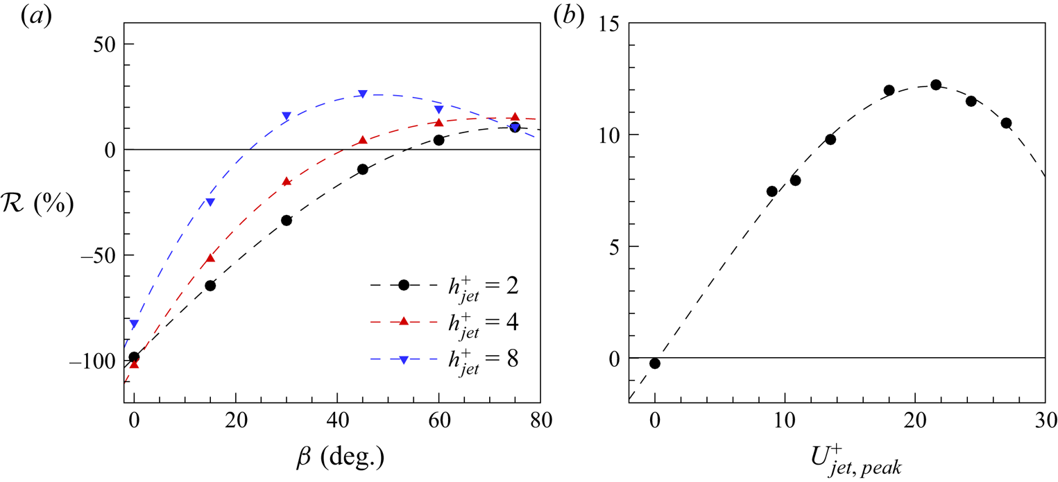
 $8$ are shown in figure 24(a). Increasing the slot height enhances the drag-reduction effect, and the largest drag reduction is achieved for
 $h^+_{jet}=8$ at a smaller optimal SJS angle than for
 $h^+_{jet}=2$, that is,
 $\mathcal {R}$=26.8 % for
 $h^+_{jet} = 8$ and
 $\beta = 45^\circ$. Larger values of
 $h^+_{jet}$ imply a larger mass flow rate for the SJS actuation, which leads to a more intense opposing streamwise component near the wall and thus larger drag reduction. Although
 $h^+_{jet}=4$ and
 $8$ lead to larger drag-reduction margins than
 $h^+_{jet}=2$, they require much higher actuation power. Therefore,
 $h^+_{jet}=2$ is studied in the main text.
Drag reduction for different (a) SJS slot heights, and (b) SJS velocities.

B.2. Jet-sheet velocity
The maximum SJS velocity is changed between  $U^+_{jet,max} = 0$ and
 $U^+_{jet,max} = 27$, and the drag-reduction margin is plotted in figure 24(b). The maximum drag-reduction margin
 $\mathcal {R} = 12.2\,\%$ is obtained for
 $U^+_{jet,max} = 21.6$.
B.3. Jet-sheet period of oscillation
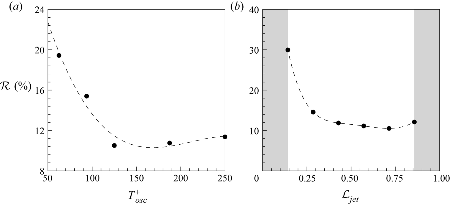
The effect of the actuation period is displayed in figure 25(a). For the tested cases, the maximum reduction is  $19.4\,\%$ for
 $T^+_{osc}=62.5$.
Drag reduction for different (a) SJS periods, and (b) lengths of jet walls.

B.4. Length of jet wall
Different  $\mathcal {L}_{jet} = L^+_{jet}/(L^+_{step} + L^+_{jet})$ values are tested by using the same number of devices in the channel and the same dimensions of the computational domain. As shown in figure 25(b), values of
 $\mathcal {L}$ that are too close to 0 and 1 are not investigated. Values too close to 0 would not be realistic because the distance between SJS would be too small, while values too close to 1 would render
 $L^+_{step}$ too short because there would not be enough space for the vanes under the steps to generate the SJS. The largest drag-reduction margin is
 $30.0\,\%$ for
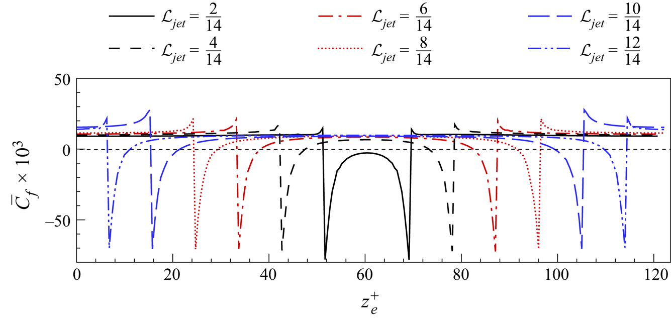
 $\mathcal {L}_{jet} = 2/14$. The spanwise distribution of the skin-friction coefficient is plotted in figure 26 for different
 $\mathcal {L}_{jet}$ values. The friction drag is reduced dramatically on the jet wall for
 $\mathcal {L}_{jet} = 2/14$ because the SJS are very close to each other and interact. The other cases of different
 $\mathcal {L}_{jet}$ values present almost the same drag-reduction margin on the jet wall. On the step wall, the friction drag is increased the most for
 $\mathcal {L}_{jet} = 10/14$.
Comparison of time and spatially averaged skin-friction distribution along the spanwise direction for different length ratios.

Appendix C. Power balance in the cavity chambers
The integral power balance of air inside the two cavity chambers is derived herein (Panton Reference Panton2013). The control volume is fixed in time and bounds the two cavity chambers, as shown in figure 13. We derive the integral mechanical power equation and the integral equation for the internal energy per unit time, and then we sum these two equations to find the integral equation for the total power.
C.1. Mechanical power in the cavity chambers
We start by performing the scalar product of the velocity  $\boldsymbol {u}$ and the compressible Navier–Stokes equations:
 \begin{equation} \rho\,\frac{{\rm D}}{{\rm D} t} \left(\frac{\vert \boldsymbol{u} \vert^2}{2}\right) ={-} \boldsymbol{u} \boldsymbol{\cdot} \boldsymbol{\nabla} p + \frac{1}{Re_p}\,\boldsymbol{u} \boldsymbol{\cdot} \left(\boldsymbol{\nabla} \boldsymbol{\cdot} \boldsymbol{\underline{\tau}}\right), \end{equation}
where  $D/D t$ denotes the material derivative, and
 $\boldsymbol {\underline {\tau }}$ is the stress tensor. By using vector and tensor identities, (C1) is written as
 \begin{equation} \rho\,\frac{{\rm D}}{{\rm D} t} \left(\frac{\vert \boldsymbol{u} \vert^2}{2}\right) = p (\boldsymbol{\nabla} \boldsymbol{\cdot} \boldsymbol{u}) -\boldsymbol{\nabla} \boldsymbol{\cdot} (p \boldsymbol{u}) + \frac{1}{Re_p}\, \boldsymbol{\nabla} \boldsymbol{\cdot} ( \boldsymbol{\underline{\tau}} \boldsymbol{\cdot} \boldsymbol{u}) - \frac{1}{Re_p}\,\boldsymbol{\underline{\tau}} : \boldsymbol{\nabla} \boldsymbol{u}, \end{equation}
where the symbol  $:$ is the contraction. By using the continuity equation, the left-hand side of (C2) expands as
 \begin{equation} \frac{{\partial}}{{\partial} t} \left(\rho\,\frac{\vert \boldsymbol{u} \vert^2}{2}\right)+ \boldsymbol{\nabla} \boldsymbol{\cdot} \left(\rho \boldsymbol{u}\,\frac{\vert \boldsymbol{u} \vert^2}{2} \right) = p (\boldsymbol{\nabla} \boldsymbol{\cdot} \boldsymbol{u}) - \boldsymbol{\nabla} \boldsymbol{\cdot} (p \boldsymbol{u}) + \frac{1}{Re_p}\, \boldsymbol{\nabla} \boldsymbol{\cdot} ( \boldsymbol{\underline{\tau}} \boldsymbol{\cdot} \boldsymbol{u}) - \frac{1}{Re_p}\,\boldsymbol{\underline{\tau}} : \boldsymbol{\nabla} \boldsymbol{u}. \end{equation}
Equation (C3) is integrated over a control volume  $V$, and by using the divergence theorem, one finds
 \begin{align} & \int_V \frac{{\partial}}{{\partial} t} \left(\rho\,\frac{\vert \boldsymbol{u} \vert^2}{2}\right) \mathrm{d}V + \int_A \rho\,\frac{\vert \boldsymbol{u} \vert^2}{2}\,\boldsymbol{u} \boldsymbol{\cdot} \boldsymbol{n} \,\mathrm{d}A = \int_V p (\boldsymbol{\nabla} \boldsymbol{\cdot} \boldsymbol{u})\,\mathrm{d}V - \int_A p \boldsymbol{u} \boldsymbol{\cdot} \boldsymbol{n}\,\mathrm{d}A \nonumber\\ &\quad +\frac{1}{Re_p}\int_A (\boldsymbol{\underline{\tau}} \boldsymbol{\cdot} \boldsymbol{u}) \boldsymbol{\cdot} \boldsymbol{n}\,\mathrm{d}A -\frac{1}{Re_p}\int_V \boldsymbol{\underline{\tau}} : \boldsymbol{\nabla} \boldsymbol{u}\,\mathrm{d}V, \end{align}
where  $A$ is the surface of the control volume
 $V$, and
 $\boldsymbol {n}$ is the unit vector pointing out of the surface
 $A$. Using the Reynolds transport theorem, (C4) is written as
 \begin{align} & \frac{\mathrm{d}}{\mathrm{d} t} \int_V \rho\,\frac{\vert \boldsymbol{u} \vert^2}{2}\,\mathrm{d}V ={-}\int_A \rho\,\frac{\vert \boldsymbol{u} \vert^2}{2}\,\boldsymbol{u} \boldsymbol{\cdot} \boldsymbol{n}\,\mathrm{d}A -\int_A p \boldsymbol{u} \boldsymbol{\cdot} \boldsymbol{n}\,\mathrm{d}A + \frac{1}{Re_p}\int_{A_{fluid}} (\boldsymbol{\underline{\tau}} \boldsymbol{\cdot} \boldsymbol{u}) \boldsymbol{\cdot} \boldsymbol{n}\,\mathrm{d}A \nonumber\\ &\quad +\frac{1}{Re_p}\int_{A_{solid}} (\boldsymbol{\underline{\tau}} \boldsymbol{\cdot} \boldsymbol{u}) \boldsymbol{\cdot} \boldsymbol{n}\,\mathrm{d}A + \int_V p (\boldsymbol{\nabla} \boldsymbol{\cdot} \boldsymbol{u})\,\mathrm{d}V-\frac{1}{Re_p} \int_V \boldsymbol{\underline{\tau}} : \boldsymbol{\nabla} \boldsymbol{u}\,\mathrm{d}V, \end{align}
where the term involving the stress tensor has been split into two terms, one involving the shear stresses at the fluid part of  $A$, and one involving the shear stresses at the solid part of
 $A$. The surface-integrated pressure work term in (C5) is split into two terms by introducing the work per unit time that is exchanged by the fluid at the SJS apertures, and the work per unit time performed by the piston against the fluid pressure over the piston area
 $A_{piston}$. The first term on the right-hand side of (C5) simplifies because only the fluid portion of
 $A$ at the SJS apertures contributes to the balance. Equation (C5) becomes
 \begin{align} & \underbrace{\frac{\mathrm{d}}{\mathrm{d} t} \int_V \rho\, \frac{\vert \boldsymbol{u} \vert^2}{2} \mathrm{d}V }_{\mathrm{d}\mathcal{E}_m/\mathrm{d}t} ={-}\underbrace{\int_{A_{fluid}} p \boldsymbol{u} \boldsymbol{\cdot} \boldsymbol{n}\,\mathrm{d}A }_{\mathcal{P}_{fluid}} -\underbrace{\int_{A_{fluid}} \rho\,\frac{\vert \boldsymbol{u} \vert^2}{2}\,\boldsymbol{u} \boldsymbol{\cdot} \boldsymbol{n}\,\mathrm{d}A }_{\mathcal{F}_{m-fluid}} + \underbrace{\frac{1}{Re_p} \int_{A_{fluid}} (\boldsymbol{\underline{\tau}} \boldsymbol{\cdot} \boldsymbol{u}) \boldsymbol{\cdot} \boldsymbol{n}\,\mathrm{d}A}_{\mathcal{T}_{fluid}} \nonumber\\ &\quad +\underbrace{\int_V p (\boldsymbol{\nabla} \boldsymbol{\cdot} \boldsymbol{u})\,\mathrm{d}V}_{\mathcal{C}} - \underbrace{\frac{1}{Re_p}\int_V \boldsymbol{\underline{\tau}} : \boldsymbol{\nabla} \boldsymbol{u}\,\mathrm{d}V}_{\mathcal{D}} - \underbrace{w_{{piston}}(t)\int_{A_{piston}} \Delta p_{{piston}}\,\mathrm{d}A}_{\mathcal{W}_{{piston}}}. \end{align}
The physical meanings of the terms in (C6) are as follows.
(i)
$\mathrm {d}\mathcal {E}_m/\mathrm {d}t$ is the time rate of change of the volume-integrated kinetic energy of the fluid inside the control volume.(ii)
$\mathcal {P}_{fluid}$ is the work per unit time performed by the fluid pressure as the fluid passes through the SJS apertures.(iii)
$\mathcal {F}_{m-fluid}$ is the flux of kinetic energy per unit time as the fluid passes through the SJS apertures.(iv)
$\mathcal {T}_{fluid}$ is the work per unit time performed by the fluid shear stresses as the fluid passes through the SJS apertures.(v)
$\mathcal {C}$ is the work per unit time performed to compress the fluid.(vi)
$\mathcal {D}$ is the dissipation per unit time of kinetic energy per unit time into heat due to viscous shear stresses.(vii)
$\mathcal {W}_{{piston}}$ is the work per unit time exerted by the piston on the fluid in the cavity chambers.


C.2. Internal energy per unit time in the cavity chambers
The equation of internal energy per unit time, from (5.10.3) in Panton (Reference Panton2013), reads
 \begin{equation} \rho\,\frac{{\rm D} e}{{\rm D} t} = \frac{{\partial} (\rho e)}{{\partial} t} + \boldsymbol{\nabla} \boldsymbol{\cdot}(\rho \boldsymbol{u} e) ={-} p (\boldsymbol{\nabla} \boldsymbol{\cdot} \boldsymbol{u}) + \frac{1}{Re_p}\,\boldsymbol{\nabla} \boldsymbol{\cdot} (k\,\boldsymbol{\nabla} T) + \frac{1}{Re_p}\,\boldsymbol{\underline{\tau}} : \boldsymbol{\nabla} \boldsymbol{u}, \end{equation}
where  $\rho e=\rho ^* e^*/(\rho _c^* U_p^{*2})$ is the scaled internal energy per unit volume,
 $T=T^*/T^*_c$ is the temperature scaled by the reference temperature of the channel flow
 $T^*_c$,
 $k= k^* \mu _c^* U_p^{*2}/T^*_c$ is the scaled thermal conductivity of air in the channel, and
 $\mu _c^*$ is the reference dynamic viscosity of air in the channel. The volume-integrated left-hand side of (C7) transforms as
 \begin{equation} \int_V \rho\,\frac{{\rm D} e}{{\rm D} t}\,\mathrm{d}V = \int_V \boldsymbol{\nabla} \boldsymbol{\cdot}(\rho \boldsymbol{u} e)\,\mathrm{d}V + \int_V \frac{{\partial} (\rho e)}{{\partial} t}\,\mathrm{d}V= \int_A \rho e \boldsymbol{u} \boldsymbol{\cdot} \boldsymbol{n}\,\mathrm{d}A + \frac{\mathrm{d}}{\mathrm{d} t} \int_V \rho e\,\mathrm{d}V \end{equation}
by expanding the material derivative and by using the divergence and the Reynolds transport theorem. By substituting (C8) into the volume-integrated (C7), and using the divergence theorem, one finds
 \begin{align} & \underbrace{\frac{\mathrm{d}}{\mathrm{d} t} \int_V \rho e\,\mathrm{d}V}_{\mathrm{d}\mathcal{E}_i/\mathrm{d}t} ={-} \underbrace{\int_{A_{fluid}} \rho e \boldsymbol{u} \boldsymbol{\cdot} \boldsymbol{n}\,\mathrm{d}A}_{\mathcal{F}_{i-fluid}} - \underbrace{\int_V p (\boldsymbol{\nabla} \boldsymbol{\cdot} \boldsymbol{u})\,\mathrm{d}V}_{\mathcal{C}} \nonumber\\ &\quad +\underbrace{\frac{1}{Re_p} \int_A k\,\boldsymbol{\nabla} T \boldsymbol{\cdot} \boldsymbol{n}\,\mathrm{d}A}_{\mathcal{Q}} + \underbrace{\frac{1}{Re_p} \int_V \boldsymbol{\underline{\tau}} : \boldsymbol{\nabla} \boldsymbol{u}\,\mathrm{d}V}_{\mathcal{D}}. \end{align}
The physical meanings of the terms in (C9) are as follows.
(i)
$\mathrm {d}\mathcal {E}_i/\mathrm {d}t$ is the time rate of change of the volume-integrated internal energy of the fluid inside the control volume.(ii)
$\mathcal {F}_{i-fluid}$ is the flux of internal energy per unit time as the fluid passes through the SJS apertures.(iii)
$\mathcal {Q}$ is the heat transfer through the surface of the control volume.


C.3. Total power balance in the cavity chambers
The balance equation for the integral total power, given by the sum of the integral mechanical power and the internal energy per unit time,  $\mathcal {E}=\mathcal {E}_m+\mathcal {E}_i$, is obtained by adding (C6) and (C9):
 \begin{align} & \underbrace{
\frac{\mathrm{d}}{\mathrm{d} t} \int_V \rho \left(e +
\frac{\vert \boldsymbol{u} \vert^2}{2} \right)
\mathrm{d}V}_{\mathrm{d}\mathcal{E}/\mathrm{d}t}
={-}\underbrace{ \int_{A_{fluid}} p \boldsymbol{u}
\boldsymbol{\cdot} \boldsymbol{n}\,\mathrm{d}A
}_{\mathcal{P}_{fluid}} -\underbrace{ \int_{A_{fluid}} \rho
e \boldsymbol{u} \boldsymbol{\cdot}
\boldsymbol{n}\,\mathrm{d}A }_{\mathcal{F}_{i-fluid}}
\nonumber\\ &\quad -\underbrace{ \int_{A_{fluid}}
\rho\,\frac{\vert \boldsymbol{u}
\vert^2}{2}\,\boldsymbol{u} \boldsymbol{\cdot}
\boldsymbol{n}\,\mathrm{d}A }_{\mathcal{F}_{m-fluid}}-
\underbrace{w_{{piston}}(t)\int_{A_{piston}} \Delta
p_{{piston}}\,\mathrm{d}A}_{\mathcal{W}_{{piston}}} +
\underbrace{\frac{1}{Re_p}\int_{A_{fluid}}
(\boldsymbol{\underline{\tau}} \boldsymbol{\cdot}
\boldsymbol{u}) \boldsymbol{\cdot}
\boldsymbol{n}\,\mathrm{d}A}_{\mathcal{T}_{fluid}}
\nonumber\\ &\quad
+\underbrace{\frac{1}{Re_p} \int_A
k\,\boldsymbol{\nabla} T \boldsymbol{\cdot}
\boldsymbol{n}\,\mathrm{d}A}_{\mathcal{Q}}.
\end{align}
The compression term  $\mathcal {C}$ and the dissipation term
 $\mathcal {D}$ cancel out because they both appear in (C6) and (C9) with opposite signs.