3.1. Derivation of the plane-average mean equation

We consider the plane-averaged streamwise Navier–Stokes equation

(3.1) \begin{equation} \langle a_u \rangle = -P_x+\nu \langle u_{yy}\rangle , \end{equation}

where $a_u \equiv u_t + u_j u_{x_j}$ (with sum over $j=1,2,3$ ) is the fluid particle acceleration comprised of Eulerian acceleration plus nonlinear advection, $u_{yy}$ is the second-order partial derivative of $u=u_1$ with respect to $y=x_2$ , $P_x$ is the $x{-}z$ plane-averaged pressure gradient (implicitly normalised by density and independent of $y$ ), $u_{x_j}$ is the partial derivative of streamwise velocity $u=u_1$ with respect to $x_{j}$ , $u_t$ is the partial derivative of $u=u_1$ with respect to time, $\nu$ is the kinematic viscosity, and the brackets represent averaging in a wall-parallel $x{-}z$ plane, i.e. $\langle A \rangle = ({1}/({L_x L_z})) \iint A \, \mathrm{d}x\,\mathrm{d}z$ . (The wall-parallel diffusion term averages to zero due to periodicity in the wall-parallel boundary conditions.) We now multiply both sides of (3.1) at arbitrary $y$ by $\nu \langle u_y \rangle (y) = \nu ({\partial }/{\partial y})\langle u \rangle (y)$ at a given $y$ , and integrate the equation in the $y$ direction from $y=0$ at the wall to some arbitrary $y$ :

(3.2) \begin{eqnarray} \nu \int _0^y \langle u_y \rangle \langle a_u \rangle \, \mathrm{d}y' &=& -\nu \int _0^y \langle u_y \rangle P_x \, \mathrm{d}y' + \frac {1}{2}\left [\nu ^2\langle u_y \rangle ^2(y,t) - \nu ^2\langle u_y \rangle ^2(y=0) \right ]\nonumber \\ \Rightarrow\quad \langle \tau _w\rangle ^2(t) &=& -2\nu \int _0^y \langle u_y \rangle \langle a_u \rangle \, \mathrm{d}y' -2\nu P_x \langle u \rangle (y,t) + \nu ^2\langle u_y \rangle ^2(y,t). \end{eqnarray}

We obtain this exact formula (3.2) for the time-fluctuating plane-averaged WSS as a sum of three different quantities that depend on wall-normal distance $y$ from the bottom wall. As the left-hand side of (3.2) is independent of $y$ , the $y$ -dependencies of the right-hand side terms cancel at every $y$ . When taking $y=0$ on the right-hand side, this relation reduces to the definition of the local WSS, i.e. $\tau _w (x,z,t) \equiv \nu\, u_y (x, y=0,z,t)$ , with vanishing shear-acceleration term and pressure-velocity term.

Figure 1.

Contributions to the square plane-average WSS: (a–c) the terms on the right-hand side of (3.2); (d) the $ \textit{Re}_\tau$ scaling of the pressure-velocity term. In each plot and in the following figures with line plots, darker lines represent data obtained from higher Reynolds numbers.

Defining the time average $ \overline {A} = \lim _{T\to \infty } ({1}/{T})\int _0^T A (t)\, \mathrm{d}t$ for any variable $A(t)$ , the time-averaged terms on the right-hand side of (3.2) are plotted in figures 1(a–c). When presented with superscript $+$ , the results are normalised by the usual inner units, i.e. the friction velocity $u_\tau$ defined from the space–time average WSS $u_\tau ^2 = \overline {\langle \tau _w \rangle }$ , and the viscous wall unit $\delta _\nu = \nu / u_\tau$ . From (3.2), the sum of the three quantities plotted in figures 1( $a{-}c$ ) equals $\overline {\langle \tau _w\rangle ^2}/u_{\tau }^{2}$ , which is very close to 1.

The term on the left-hand side of (3.2) comprises both the mean (time-averaged) and the time-fluctuating part of the plane-averaged WSS. The time fluctuation of $\langle \tau _w\rangle (t)$ in terms of rms is less than 5 % of its time-average value for all five Reynolds numbers. Therefore, the time-average squared WSS contain less than 0.25 % deviation, which is insignificant compared to the square of the time-average WSS ( $\overline {\langle \tau _w\rangle ^2}/u_{\tau }^{2}-1 \lt 0.0025$ ). Numerical integration in the wall-normal direction is performed with the cubic spline method, and the resulting numerical error is within 1 % of the square mean WSS.

3.2. Estimate of WSS and Reynolds number dependencies

The time-average square mean shear stress $\overline { \langle {u_y^+} \rangle ^2 } = \overline {\langle {u_y} \rangle ^2} \,{\delta _\nu ^2}/{u_\tau ^2}$ normalised by inner units shown in figure 1( $c$ ) is nearly equal to 1 at the wall, and reduces monotonically as $y$ increases further away from the wall. 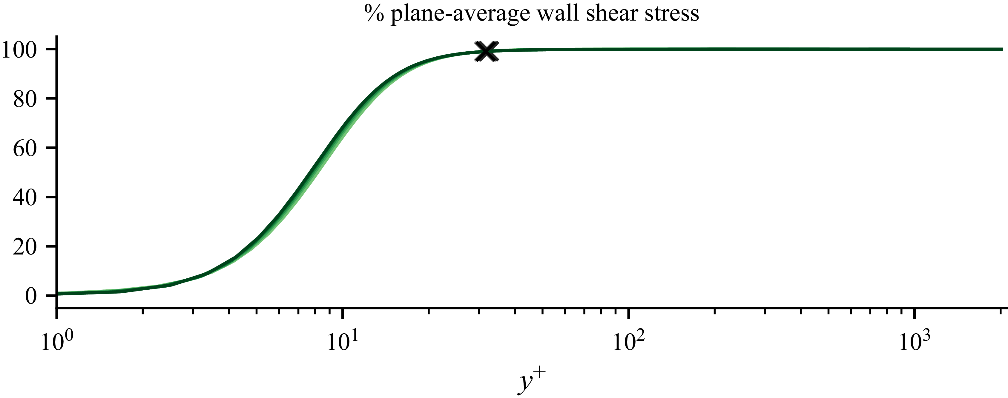At $y^+\approx {31}$ , $\overline { \langle {u_y^+} \rangle ^2}$ drops below 1 % of the time-average square WSS $\overline { \langle \tau _w\rangle ^2}/u_{\tau }^{4}$ for all five Reynolds numbers. Due to the exact balance in (3.2), the other two terms, namely the shear-acceleration and shear-pressure terms, contribute to 99 % of the mean square WSS. Similar to the $\delta _{99}$ definition for the turbulent boundary layer thickness, we may define a position $\delta _w = \delta _{1\,\%} \equiv 31 \delta _\nu$ as a cut-off wall-normal position. Changing the cut-off threshold, the 0.2 % cut-off position is approximately $54 \delta _\nu$ , for example. This cut-off position identifies the $y$ -location above which only the shear-acceleration term plotted in figure 1( $a$ ) and the pressure-velocity term plotted in figure 1( $b$ ) effectively (if not overwhelmingly) contribute to $\overline { \langle \tau _w\rangle ^2}$ . (Note that the local contribution from the molecular shear stress vanishes beyond this cut-off position, as plotted in figure 1( $c$ ).) The dominance of these two contributions to $\overline { \langle \tau _w\rangle ^2}$ is confirmed by figure 2, where we plot the percentage contribution to $\overline { \langle \tau _w\rangle ^2}$ from these two terms as a function of the upper $y$ limit of the integral. It is found that the corresponding curves for the five Reynolds numbers collapse rather well, but not perfectly. The cut-off position $\delta _w$ for estimating the mean square WSS, indicated as cross symbols in figure 2, collapses well for the five Reynolds numbers. By taking the definition of the buffer layer to reach up to the distance from the bottom wall where average turbulence production starts approximately balancing average turbulence dissipation (at $y^+\approx 60$ ; see e.g. figure 8 in Yin et al. Reference Yin, Hwang and Vassilicos2024), this result suggests that the viscous and buffer layers within a distance $\delta _w$ from the wall encode within them all the necessary information required to calculate the plane-average WSS (García García & Fariñas Alvariño (Reference García García and Fariñas Alvariño2022) make a similar claim for pipe flow in a different way). This does not mean that the plane-average WSS are not influenced by the flow far from the wall; it just means, as further explained below, that it can be calculated using information about the flow (specifically, the mean flow gradient and the mean streamwise fluid acceleration) within the viscous and buffer layers only, i.e. within a distance $\delta _w$ from the wall, where $\delta _w$ scales with $\delta _{\nu }$ .

To better appreciate this result, it may help to spell out the differences between (3.2) and the usual integrated mean momentum equation obtained by directly integrating (3.1) over  $y$ :

(3.3) \begin{equation} \langle \tau _w\rangle = -\int _{0}^{y} \langle a_u \rangle \, \mathrm{d}y' - P_x y +\nu \langle u_{y}\rangle (y,t). \end{equation}

The integrand $\langle u_y \rangle \langle a_u \rangle$ in the first term of the right-hand side of (3.2) decays to zero with increasing $y'$ , whereas the integrand $\langle a_u \rangle$ in the first term of the right-hand side of (3.3) does not. In particular, time averaging of both sides of (3.3) leads to $\overline {\langle \tau _w\rangle } = -\overline {\langle u v\rangle } (y) - \overline {P_x} y +\nu \overline {\langle u_{y}\rangle } (y)$ which makes it clear that $\int _{0}^{y} \overline {\langle a_u \rangle }\, \mathrm{d}y' = \overline {\langle u v\rangle } (y)$ does not tend to become independent of $y$ with increasing $y$ , as it would if $\overline {\langle a_u \rangle }$ decayed to $0$ fast enough with increasing $y'$ . Hence whilst the first term on the right-hand side of (3.2) does not grow with $y$ above $\delta _w$ , the first term on the right-hand side of (3.3) does, and this is particularly clear from the time-averaged form of (3.3) where $-\overline {\langle u v\rangle } (y)$ continues growing until $y$ reaches $y_{m} \sim \sqrt {\delta _{\nu } \delta }$ . Indeed, the wall distance $y_{m} \sim \sqrt {\delta _{\nu } \delta }$ where $-\overline {\langle u v\rangle }$ is maximal follows directly by assuming a log law for $\overline {\langle u \rangle }$ (see e.g. Afzal Reference Afzal1984; Panton Reference Panton2007; Lee & Moser Reference Lee and Moser2015; Hwang & Lee Reference Hwang and Lee2020). This length scale $\sqrt {\delta _{\nu } \delta }$ characterises the mesolayer (Afzal Reference Afzal1984), and at high enough Reynolds numbers is larger than $\delta _{w}$ , which scales with $\delta _{\nu }$ . Note that the linear dependence on $y$ of the pressure term on the right-hand side of (3.3) is essential for obtaining this mesolayer length scale, and that the dependence on $y$ of the pressure term on the right-hand side of (3.2) is much weaker than linear. Given these important differences between the integrated momentum equation (3.3) and our (3.2), it is necessary to integrate terms in (3.3) from the wall up to the channel centre to calculate the plane-average WSS, while relation (3.2) encodes all necessary information required to calculate the plane-average WSS within the viscous and buffer layers only.

Figure 2.

Percentage contribution from shear-acceleration plus shear-pressure-gradient to mean WSS. Results from five Reynolds numbers collapse rather well. The overlapping cross symbols indicate the $\delta _w$ in the estimate (3.5) that reaches $99\,\%$ of the mean square WSS for all five Reynolds numbers.

We now focus on the terms on the right-hand side of (3.2). While $\overline { \langle {u_y^+} \rangle ^2}$ shows little Reynolds number dependence close to the wall (figure 1 $c$ ), both the shear-acceleration and the pressure-velocity terms show significant Reynolds number effects (figures 1 $a,b$ ). The latter’s Reynolds number dependence can be estimated as follows. In a constant mass flux channel, the plane-average pressure gradient balances the sum of the plane integrals of WSS on the two walls instantaneously. By assuming that the plane-average pressure gradient does not correlate heavily in time with the plane-average velocity profile, one can estimate the mean pressure gradient as the squared friction velocity divided by the channel half-height, i.e.

(3.4) \begin{equation} -\nu\, \overline {P_x \langle u \rangle } /u_\tau ^4 \approx \ \frac {\nu \overline {\langle u \rangle } u_\tau ^2 }{ u_\tau ^4 \delta } =\ \frac {\overline {\langle u \rangle }}{u_\tau } \frac {\nu }{\delta u_\tau } =\ \frac {U^+(y^{+})}{Re_\tau }, \end{equation}

where $U^+(y^{+})$ is the mean velocity profile scaled in inner units, which may be assumed to be invariant with Reynolds number in the near-wall region. We therefore plot in figure 1( $d$ ) the pressure velocity term multiplied by $ \textit{Re}_\tau$ . The product collapses approximately for all five Reynolds numbers. The slight mismatch between the proposed scaling and the data from the current simulation may be due to two main possible causes: time correlations between the time fluctuations of the plane-average pressure gradient and the plane-average velocity, which, as we checked for R230, reduce with increasing computational domain size; and residual weak Reynolds number effects on the mean velocity profile. We note that the above balance would be exact in a constant pressure gradient channel (with $\approx$ replaced by $=$ ).

At high enough Reynolds number, we therefore have the following estimation of the time-average square mean WSS in terms of the product between the mean shear and the plane-average acceleration integrated from the wall to some finite distance from the wall, plus a correcting pressure-velocity term that is proportional to $1/Re_\tau$ (this estimate is acceptable even without time averaging):

(3.5) \begin{equation} \overline {\langle \tau _w\rangle ^2} \approx -2\nu \int _0^{\delta _w} \overline {\langle u_y \rangle \langle a_u \rangle } \, \mathrm{d}y' + O(1/Re_\tau ). \end{equation}

This result signifies the existence of a cut-off wall-normal distance $y = \delta _w$ that seems to scale with $\delta _\nu$ and beyond which there is no more additive contribution from the shear-acceleration term to $\overline {\langle \tau _w\rangle ^2}$ . The pressure-gradient contribution vanishes at a $1/Re_\tau$ rate at large Reynolds numbers. Once sufficient information regarding the plane-average acceleration and shear near the wall (viscous and buffer layers) is gathered, it is possible to estimate $\overline {\langle \tau _w\rangle ^2}$ exclusively based on near-wall data. Note, however, that $\delta _w /\delta _\nu$ may have a weak dependence on $ \textit{Re}_\tau$ that cannot be captured with the range of Reynolds numbers of our DNS data sets, which may imply that information regarding the plane-average acceleration and shear may also be required from above the buffer layer at some enormous value of $ \textit{Re}_\tau$ .

Figure 3.

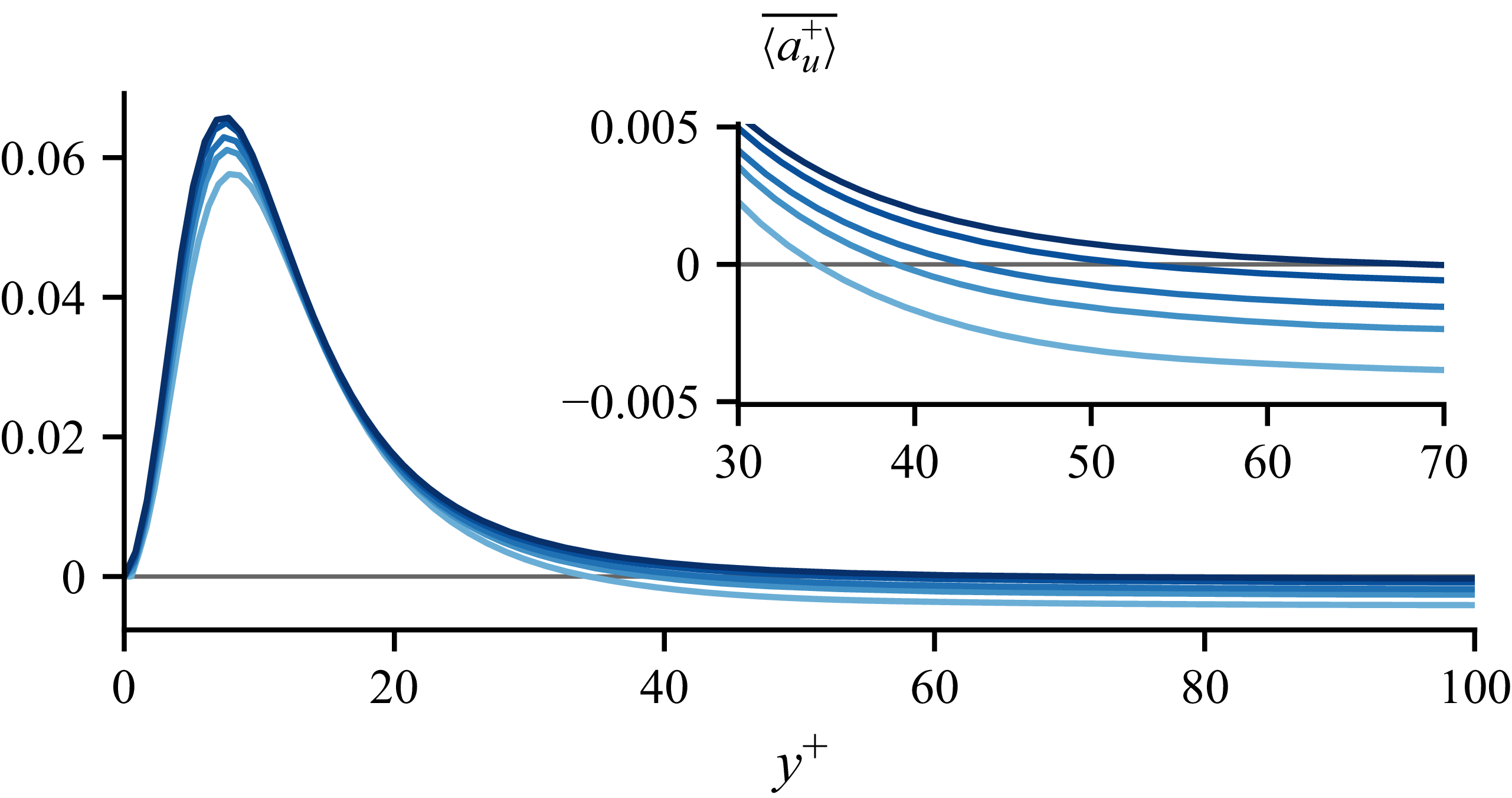
Mean acceleration profile.

As all indications to date are that the mean skin-friction coefficient has a weak dependence on $ \textit{Re}_\tau$ with increasing $ \textit{Re}_\tau$ , one may also expect $\overline {\langle \tau _w\rangle ^2}$ to have such an asymptotic dependence. This dependence may come either from a $ \textit{Re}_\tau$ dependence of $\delta _w /\delta _\nu$ , which is beyond our reach in this paper, or from the $ \textit{Re}_\tau$ dependence of the integrand in the integral on the right-hand side of (3.5), or both. The plane-average shear profile $ \langle u_y \rangle$ may be considered as almost fully scaling in inner units near the wall. (This is reminiscent of the law of the wall, which states that the time- and plane-average shear profile $\overline {\langle u_y \rangle }$ fully scales in inner units near the wall.) However, the plane-average acceleration $\langle a_u \rangle$ (figure 3) is composed of the plane-average Eulerian acceleration and the Reynolds shear stress gradient, the latter clearly depending on Reynolds number. Even in the minimal computational domain, the plane-average Eulerian acceleration is less than $1\,\%$ of the plane-average Reynolds shear stress gradient. The gradient of Reynolds shear stress is known to cross zero (local maximum of Reynolds shear stress) at a $y^+$ value that increases with Reynolds number. Reynolds number dependencies in magnitude and in zero-crossing location are clearly shown in figure 3, where we plot the wall-normal profile of $\overline {\langle a_u \rangle }$ in inner coordinates. If $\delta _w /\delta _\nu$ is independent of $ \textit{Re}_\tau$ , then all the information required to calculate $\overline {\langle \tau _w\rangle ^2}$ from the fluid flow can be found between the wall and the outer edge of the buffer layer for any Reynolds number. However, this thin near-wall region will then need to be Reynolds number dependent if $\overline {\langle \tau _w\rangle ^2}$ is Reynolds number dependent, and this Reynolds number dependence will reflect a dependence of this thin near-wall region on the outer flow.

4.1. Formula for the WSS variance and time-average statistics

We consider the fluctuating streamwise momentum equation (obtained by subtracting the plane-average streamwise momentum equation (3.1) from the total equation):

(4.2) \begin{equation} a_u' = -p_x'+\nu\, {\nabla} ^2 u'. \end{equation}

We first multiply the above equation by $\nu u_y'$ , average over the $x$ – $z$ plane, and integrate in the wall-normal direction from the wall to some arbitrary $y$ , and using (4.1), we obtain

(4.3) \begin{equation} \langle \tau _w'^2\rangle = -2\nu \int ^y_0 \langle u'_y a_u'\rangle \, \mathrm{d}y' -2\nu \int ^y_0 \langle u'_y p_x' \rangle \, \mathrm{d}y' + 2\nu ^2\int ^y_0 \langle u'_y u_{//}' \rangle \, \mathrm{d}y' + \nu ^2 \langle {u'_y} ^2\rangle , \end{equation}

where $a_u'$ is the fluctuating acceleration (see § 4.3), $p_x'$ is the fluctuating streamwise pressure gradient (implicitly normalised by the density), $u_{//}' = u_{xx}'+u_{zz}'$ is the sum of the second derivatives in the $x$ and $z$ directions of the streamwise velocity, and $\tau _w' \equiv \nu\, u_y'(y=0)$ is the fluctuating WSS that appears from the vertical momentum diffusion term. To the authors’ knowledge, this is the first exact relation describing the spatially fluctuating WSS directly using the Navier–Stokes equations. We note that an equation for the spanwise component of the WSS can be similarly derived from the fluctuating spanwise momentum equation. However, the relation between the streamwise and spanwise WSS is beyond the scope of the present study.

Figure 5.

Contributions to the variance of WSS in (4.3).

Figure 5. Long description

Panel A: A line graph shows the integral of the product of fluctuations in wall-normal velocity and wall shear stress against the wall-normal coordinate. The x-axis is labeled y+ and ranges from 0 to 200. The y-axis ranges from 0 to 0.2. Multiple lines in blue represent different Reynolds numbers. Panel B: A line graph shows the integral of the product of fluctuations in wall-normal velocity and pressure against the wall-normal coordinate. The x-axis is labeled y+ and ranges from 0 to 200. The y-axis ranges from -0.05 to 0.025. Multiple lines in green represent different Reynolds numbers. Panel C: A line graph shows the variance of wall-normal velocity fluctuations against the wall-normal coordinate. The x-axis is labeled y+ and ranges from 0 to 200. The y-axis ranges from 0 to 0.15. Multiple lines in red represent different Reynolds numbers. Panel D: A line graph shows the integral of the product of fluctuations in wall-normal velocity and streamwise velocity against the wall-normal coordinate. The x-axis is labeled y+ and ranges from 0 to 200. The y-axis ranges from -0.03 to 0. The line in black represents different Reynolds numbers.

The wall-normal profile of each time-averaged budget term on the right-hand side of (4.3) is plotted in figure 5 normalised in inner units. The major contribution to the WSS fluctuations far enough from the wall is the positive contribution from the integrated shear-acceleration covariance attenuated by the negative contribution from the integrated shear-pressure-gradient covariance at normalised wall distances $y^+$ below 100. The latter contribution turns from negative to positive at $y^+ \approx 100$ , but remains relatively minor at $y^+ \gt 100$ . The two terms on the right-hand side of (4.3) stemming from viscous diffusion diminish in magnitude with wall distance, and appear to quickly become negligible, as shown in figures 5( $c{,}d$ ). Whilst the profiles of these two viscous diffusion-related terms collapse rather well in inner units (except very near the wall for $\nu ^2 \langle {u'_y} ^2\rangle$ ), the two main contributions to $\langle \tau _w'^2\rangle$ display a significant increase in magnitude with increasing $ \textit{Re}_{\tau }$ in figures 5( $a{,}b$ ), where they are plotted in inner units. The magnitude of the negative integrated shear-pressure-gradient covariance increases at $y^+\approx 20$ with increasing Reynolds number, as opposed to the diminishing contribution of the plane-average pressure-velocity term to the mean WSS.

The major contribution to both the plane-average and the fluctuating WSS comes from an integral involving shear and acceleration, with some correction from the term involving pressure. We plot in figure 6 the time-averaged sum of the $y$ -integrated shear-acceleration covariance and the $y$ -integrated shear-pressure-gradient covariance as a percentage contribution to $\overline {\langle \tau _w'^2\rangle }$ . The percentage is given as a function of the upper $y$ limit of the integrals. The plotted percentage contributions of shear-acceleration and shear-pressure-gradient terms reach a plateau at some approximate $y^+\approx 30$ , similar to the observation made in figure 2. However, there is no plateau-reaching behaviour in figures 5( $a{,}b$ ) as there is in figures 1( $a{,}b$ ) so that both the shear-acceleration and the shear-pressure-gradient terms contribute significantly to the fluctuating WSS even beyond $y^+ \gt 200$ ; the percentage plotted in figure 6 does reach a plateau beyond $y^+\approx 30$ .

Figure 6.

Percentage contribution from shear-acceleration plus shear-pressure-gradient to the variance of WSS. Results from five Reynolds numbers again collapse rather well. The cross symbols that indicate $\delta _{w'}$ in the estimate (4.4) show more scatter with Reynolds number when compared to $\delta _{w}$ in the estimate (3.5) of the mean square WSS.

This observation stems from the approximate balance between fluctuating acceleration and fluctuating pressure far from the wall where fluctuating viscous diffusion is negligible (see § 4.2). As a result, we may expect the following estimate for the variance of the fluctuating WSS:

(4.4) \begin{equation} \overline {\langle {\tau _w'}^2\rangle } \approx -2\nu \int _0^{\delta _{w'}} \overline {\langle u_y' a_u' \rangle } \, \mathrm{d}y'-2\nu \int _0^{\delta _{w'}} \overline {\langle u_y' p_x' \rangle } \, \mathrm{d}y'. \end{equation}

This estimate parallels the estimate (3.5) for the mean WSS. For the Reynolds numbers accessible by our FD TCF data, the Navier–Stokes equations imply that one can predict the WSS mean and variance from statistics involving mean/fluctuating shear, acceleration and pressure gradient between the wall and the upper edge of the buffer region. Similar to the estimate (3.5), the choice of the upper limit $\delta _{w'}$ of the integral in $y$ depends on the threshold that we chose for deciding that the percentage in figure 6 is close enough to 100 %. Using cross symbols, we plot in figure 6 the upper limit $\delta _{w'}$ defined as the height where the sum of the shear-acceleration covariance and shear-pressure-gradient covariance reaches 99 % of the variance of fluctuating WSS, i.e. with 1 % difference, similar to the definition of $\delta _w$ in § 3.2. Comparing results in figures 2 and 6, the percentage contribution to the fluctuating WSS shows slightly larger variability with varying Reynolds numbers. This observation suggests that $\delta _{w'}$ in (4.4) has a slightly stronger dependence on $ \textit{Re}_\tau$ than $\delta _w$ in (3.5), as the values of $\delta _{w'}$ are slightly scattered between $29\delta _\nu$ and $34\delta _\nu$ . However, the Reynolds number dependence of $\overline {\langle {\tau _w'}^2\rangle }$ shown in figures 4( $a{,}c$ ) may also arise from the integrands in (4.4). Even so, (4.4) suggests that the variance of the fluctuating WSS is fully encoded within the buffer layer, i.e. that it is possible to obtain it from information within this layer.

In figures 7( $a$ ) and 7( $b$ ), we plot these two integrands in inner units as functions of $y^+$ . As the vertical axis is linear and the horizontal axis is logarithmic, we premultiply them by $y^+$ to ensure that the integral over $\log y^{+}$ is the same. Plotted in the same way in figure 7( $c$ ) is the spatial covariance between local shear and wall-parallel diffusion of streamwise fluctuating velocity, whose integral gives the difference between fluctuating WSS and local-in- $y$ streamwise shear (see (4.1)). The sum of the four covariances in figures 7( $a{-}d$ ) is zero at each $y^+$ , as they are exactly balanced by the streamwise momentum equation. It is not until the channel centre $y^+ = Re_\tau$ , the plane of symmetry, that the differential contribution from the shear-acceleration covariance becomes zero. The premultiplied shear-acceleration covariance (figure 5 $a$ ) and shear-pressure-gradient covariance (figure 5 $b$ ) beyond $y^+ = 30$ seem to cancel each other far enough from the wall, sharing similar positive/negative peak location at $y^+ \in [50,60]$ , as well as peak magnitudes. This observation is consistent with the integral estimate (4.4) and the integral profiles plotted in figure 5. Concerning Reynolds number dependence, a discussion that parallels the discussion at the end of § 3.2 could be repeated here for $\overline {\langle {\tau _w'}^2\rangle }$ and referring to figures 5( $a{,}b$ ), rather than $\overline {\langle \tau _w\rangle ^2}$ and referring to figure 3.

Figure 7.

Premultiplied integrand contribution to square fluctuating plane-average WSS.

Figure 7. Long description

Panel A: A line graph shows the premultiplied integrand contribution to the square fluctuating plane-average wall shear stress for different Reynolds numbers (R230, R360, R500, R950, R2000). The x-axis is labeled y+ on a logarithmic scale, and the y-axis is labeled -y+<u’_y a’_w>+. The lines show varying trends with peaks and troughs. Panel B: A line graph shows the premultiplied integrand contribution to the square fluctuating plane-average wall shear stress for different Reynolds numbers (R230, R360, R500, R950, R2000). The x-axis is labeled y+ on a logarithmic scale, and the y-axis is labeled -y+<u’_y p’_x>+. The lines show varying trends with peaks and troughs. Panel C: A line graph shows the premultiplied integrand contribution to the square fluctuating plane-average wall shear stress for different Reynolds numbers (R230, R360, R500, R950, R2000). The x-axis is labeled y+ on a logarithmic scale, and the y-axis is labeled y+<u’_y u’_yy>+. The lines show varying trends with peaks and troughs. Panel D: A line graph shows the premultiplied integrand contribution to the square fluctuating plane-average wall shear stress for different Reynolds numbers (R230, R360, R500, R950, R2000). The x-axis is labeled y+ on a logarithmic scale, and the y-axis is labeled y+<u’_y u’_ff>+. The lines show varying trends with peaks and troughs.

The observation that there is no plateau-reaching behaviour in figure 5 stems from the local balance between the fluctuating acceleration and fluctuating pressure gradient away from the wall (figures 7 $a{,}b$ ), which we discuss in § 4.2. The key contribution to the variance of WSS is the shear-acceleration correlation in the near-wall region as shown in figure 7( $a$ ). To better understand this correlation between fluctuating streamwise shear and fluctuating streamwise acceleration, in § 4.3 we decompose the fluctuating streamwise acceleration in a way which reveals cancellations caused by Taylor’s frozen eddies hypothesis, and in § 4.4 we explore the shear-acceleration covariance in detail, and reveal the origin of the near-wall peak in the shear-acceleration term.

4.2. Pressure and acceleration

The fluctuating acceleration, pressure gradient and viscous diffusion are related exactly by the fluctuating streamwise momentum equation (4.2). Approaching the wall as $y^+ \to 0$ , velocity and acceleration vanish, resulting in the balance $p_x' \approx \nu u_{yy}'$ in some typical sense sufficiently close to the wall. Further away from the wall, i.e where $y^+ \gg 1$ , the viscous diffusion, as the solenoidal part of the force (normalised by density) balancing the acceleration, becomes less and less dominant. We expect therefore $a_u' \approx -p_x'$ to typically hold away from the wall, thereby explaining the self-cancelling behaviour in figures 7( $a{,}b$ ), and the plateau behaviour in figure 6. To examine the validity of these two approximations, we plot in figures 8( $a$ ) and 8( $c$ ) the correlation coefficient between pressure gradient and vertical viscous diffusion of streamwise momentum, and the correlation coefficient between pressure gradient and streamwise acceleration, respectively. For zero-mean variables $A(x,y,z,t)$ and $B(x,y,z,t)$ fluctuating in space and time, we define a spatial correlation coefficient as

(4.5) \begin{equation} cor_{[A,B]}(y) = \overline {\left (\frac {\langle AB \rangle }{\sqrt {\langle {A}^2\rangle }\sqrt {\langle {B}^2\rangle }}\right )}. \end{equation}

Figure 8.

Pressure effect. ( $a$ , $c$ ) Correlation of streamwise pressure gradient, vertical viscous diffusion and acceleration. ( $b$ , $d$ ) Red indicates rms of pressure gradient fluctuation, and blue indicates ( $b$ ) rms of vertical viscous diffusion, ( $d$ ) rms of streamwise acceleration. All rms are normalised in inner units.

Inside the viscous sublayer and above the wall, the correlation coefficient between pressure gradient and vertical diffusion (figure 8 $a$ ) reduces quickly with distance from the wall. The correlation coefficient between pressure gradient and acceleration (figure 8 $c$ ) remains negative inside the viscous sublayer, showing very significant anti-correlation. These two observations combined indicate that inside the viscous sublayer $y^+\lt 10$ , both viscous diffusion and pressure gradient contribute to the acceleration, and the three quantities are comparable to each other in their rms (figures 8 $b{,}d$ ) and correlations. The respective rms values shown are consistent with the study of Yeo et al. (Reference Yeo, Kim and Lee2010) (see their figures 3 and 4). Significant deviations to the pressure-diffusion balance, which is actually exact at the wall, already occur extremely close to the wall as acceleration quickly develops.

In the range $10\lt y^+\lt 100$ , the rms of vertical diffusion quickly reduces, and the correlation between streamwise pressure gradient and acceleration quickly develops, attaining nearly $-1$ as an almost perfect anti-correlation. Note that this almost perfect anti-correlation can be found in isotropic turbulence even at moderate Reynolds number (e.g. see figure 4 in Tsinober et al. Reference Tsinober, Vedula and Yeung2001). Above $y^+\gt 100$ , the rms values of pressure and acceleration almost coincide. The self-cancellation between pressure gradient and acceleration, which explains the plateau behaviour in figure 6, is therefore supported by the almost perfect anti-correlation and coinciding rms values (figures 8 $c{,}d$ ), and also evidenced by the absence of viscous diffusion far from the wall (figures 8 $a{,}b$ ).

4.3. Taylor’s hypothesis

Among the four premultiplied covariances presented in figure 7, the shear-acceleration covariance provides the largest contribution to $\overline {\langle {\tau _w'}^2\rangle }$ . We investigate this primary contribution to the WSS fluctuation variance by applying the Reynolds decomposition and decomposing acceleration into five parts:

(4.6) \begin{equation} a_u' = u_t' + \langle u_j \rangle u_{x_j}' + u_j' u_{x_j}' + u_j' \langle u_{x_j} \rangle -\langle u_j' u_{x_j}' \rangle , \end{equation}

where $u_t'=({\partial }/{\partial t}) u'$ is the fluctuating acceleration in the Eulerian frame of reference, i.e. fixed with respect to the wall; $\langle u_j \rangle u_{x_j}' = \langle u \rangle u_{x}'+\langle w \rangle u_{z}'$ (with $u_{x}'$ and $u_{z}'$ standing for $({\partial }/{\partial x}) u'$ and $({\partial }/{\partial z}) u'$ , respectively) is the advection of the fluctuating velocity field by the mean field, with the mean wall-normal velocity $\langle v \rangle$ being zero in TCF (plane-averaging the continuity equation and integrating in the wall-normal direction from the wall leads to $\langle v \rangle =0$ ); $u_j' u_{x_j}'$ (with Einstein summation over $j=1,2,3$ , and $u_{x_j}'$ standing for $({\partial }/{\partial x_{j}}) u'$ ) is the self-advection of the fluctuating velocity field; $u_j' \langle u_{x_j} \rangle = v'\langle u_{y} \rangle$ (with $u_{x_j}$ standing for $({\partial }/{\partial x_{j}}) u$ ) is a term related to turbulent kinetic energy production, as it involves the interaction between the fluctuating velocity field and the mean shear; and finally $\langle u_j' u_{x_j}' \rangle$ is the plane-average Reynolds shear stress gradient, which does not correlate with fluctuating shear and therefore has no contribution in the fluctuating WSS. The premultiplied covariances between the fluctuating streamwise shear and each one of the four fluctuating components making up $a_u'$ in (4.6) are shown in figure 9. The sum of these four covariances is equal to the fluctuating shear-acceleration covariance in figure 7( $a$ ).

Figure 9.

Decomposed acceleration contributions.

Upon first observation, we notice that the magnitudes of the covariance of local shear with Eulerian acceleration (figure 9 $a$ ) and that with mean advection (figure 9 $b$ ) are opposite in sign and at least one order of magnitude larger than the overall covariance between shear and Lagrangian acceleration in figure 7( $a$ ), as if they almost cancel each other. It is therefore sensible to investigate whether and to what extent the local Eulerian acceleration of the fluctuating streamwise velocity is mainly due to local mean advection of that velocity, i.e. whether and to what extent Taylor’s frozen eddies hypothesis, $u_t' \approx - \langle u_j \rangle u_{x_j}'$ , holds.

Figure 10.

Taylor’s hypothesis tested with correlation coefficient and rms values. ( $a$ , $c$ ) Correlation of Eulerian acceleration and streamwise advection. ( $b$ , $d$ ) Here, red indicates rms of fluctuating Eulerian acceleration, and ( $b$ ) blue indicates rms of advection of fluctuating velocity by total velocity, ( $d$ ) blue indicates rms of mean advection of fluctuating velocity. All rms are normalised in inner units.

Figure 10. Long description

Panel A: A line graph shows the correlation coefficient between Eulerian acceleration and streamwise advection. The x-axis is labeled y+ on a logarithmic scale, and the y-axis ranges from -1.0 to -0.7. Multiple lines in varying shades of purple indicate different data sets. Panel B: A line graph displays the root mean square (rms) values of fluctuating Eulerian acceleration in red and the rms of advection of fluctuating velocity by total velocity in blue. The x-axis is labeled y+ on a logarithmic scale, and the y-axis ranges from 0 to 0.6. Panel C: Another line graph shows the correlation coefficient between Eulerian acceleration and streamwise advection, with the x-axis labeled y+ on a logarithmic scale and the y-axis ranging from -1.0 to -0.9. Multiple lines in varying shades of purple represent different data sets. Panel D: A line graph depicts the rms of mean advection of fluctuating velocity, with the x-axis labeled y+ on a logarithmic scale and the y-axis ranging from 0 to 0.6. Lines in varying shades of blue and red indicate different data sets.

In figure 10( $a$ ), we plot the spatial correlation coefficient between Eulerian acceleration $u_t'$ and sum of streamwise mean and self-advection $u_ju_{x_j}' = \langle u_j\rangle u_{x_j}' +u_j' u_{x_j}'$ , and in figure 10( $b$ ) we plot their respective rms values. Large negative correlation coefficients, reaching nearly $-1$ at channel centre, between the Eulerian acceleration and streamwise advection across the channel indicate strong anti-correlating behaviour far enough from the wall. This cancellation behaviour is further consolidated by their similar rms values far enough from the wall, e.g. $y^+ \gtrsim 50$ . In fact, the anti-correlation between the local Eulerian acceleration and the streamwise mean advection $\langle u \rangle u_x'$ is even stronger, as shown by the similar correlation coefficients in figure 10( $c$ ) and the rms peaks in figure 10( $d$ ), evidencing a large degree of applicability of Taylor’s hypothesis where this anti-correlation is large enough. The spanwise mean advection is very small due to the small plane-average spanwise velocity $\langle w\rangle$ , even in the current small computational domain. Removing the self-advection of fluctuating velocity field leads to stronger anti-correlation close to the wall. While the turbulent self-advection is relatively small compared to the mean advection, they still provide significant contributions to the overall shear-acceleration covariance, as shown by the magnitude of the covariance in figure 9( $c$ ) compared to that in figure 7( $a$ ).

It is noteworthy that Taylor’s frozen eddies hypothesis appears valid with correlation coefficients between $-0.85$ and $-1$ in figure 10( $c$ ) at all distances from the wall, which confirms previous correlation analyses by Piomelli et al. (Reference Piomelli, Balint and Wallace1989) and Geng et al. (Reference Geng, He, Wang, Xu, Lozano-Durán and Wallace2015). We can therefore conclude that the average convective nature of TCF testified by Taylor’s hypothesis is largely responsible for the cancellation between the covariance of local fluctuating shear with fluctuating Eulerian acceleration (figure 9 $a$ ) and the covariance of local fluctuating shear with mean advection (figure 9 $b$ ) in this region. In the definition of the correlation coefficient (4.5), the plane-average mean velocity appearing in the numerator is factored out by itself in the denominator. The choice of such plane-average velocity plays no role in the value of the coefficient. The mean streamwise velocity $\langle u \rangle$ may in fact differ from the actual convection velocity, especially in the near-wall region, as detailed by Geng et al. (Reference Geng, He, Wang, Xu, Lozano-Durán and Wallace2015). As far as covariances of fluctuating quantities are concerned, the choice of mean or convection velocity plays no role in the correlation analysis.

We have already noted that the shear-acceleration covariance in figure 7( $a$ ) provides the largest contribution to $\overline {\langle {\tau _w'}^2\rangle }$ . It has a peak close to $y^+ \approx 5$ . Among the four covariances in figure 9, only the covariance between local fluctuating shear and the turbulence production-related term displays a peak below $y^+\lt 10$ (figure 9 $d$ ). It is this peak that is reflected in the shear-acceleration covariance peak seen in figure 7( $a$ ). These two peaks not only share a similar $y^+$ location, they also display similar peak magnitudes, although the shear-acceleration covariance displays a Reynolds number dependence that is more pronounced than the shear-production covariance. We propose that it is the shear-production term in figure 9( $c$ ) that mainly determines the near-wall peak position and magnitude of the shear-acceleration covariance in figure 7( $a$ ), and that the other covariances in figures 9( $a{,}b{,}d$ ) contribute to the Reynolds number dependence.

Figure 11.

The PMI at $y^+\in [4,5]$ where the shear-production covariance $-\overline {\langle u_y\rangle \langle v'u_y'\rangle }$ maximises, for (a,c,e,g,i) $(v',u_y')$ and (b,d,f,h,j) $(v',u')$ , for cases ( $a,b$ ) R230, ( $c,d$ ) R360, ( $e,f$ ) R500, ( $g,h$ ) R950, ( $i,j$ ) R2000. All quantities are normalised by their respective rms values.

4.4. Origin of the near-wall peak

In TCF, $\langle v \rangle (y,t) = 0$ at all $y$ . Inside the $x$ – $z$ plane average of shear-production covariance $-\langle u_y\rangle \langle u_y'v' \rangle$ , one may consider the fluctuating local shear as a weight to the averaging of $v'$ . For the weighted average $-\langle u_y'v' \rangle$ to be positive within the viscous sublayer, there must e.g. be an increased chance for $u_y'$ to be large and positive wherever $v'$ is negative, i.e. the two quantities must be dependent in their joint probability density function (PDF) $P(v',u_y')$ . If they were independent of each other, then we would have $P(v',u_y') = P(v')\,P(u_y')$ , and then converting plane-averaging into expectations on the support of $v'$ and $u_y'$ gives

(4.7) \begin{align} -\langle v' u_y' \rangle = \int P(v',u_y')\, \mathrm{d}(v',u_y') =\int P(v')\,P(u_y')\, \mathrm{d}v'\,\mathrm{d}u_y' = -\langle v' \rangle \langle u_y' \rangle = 0. \end{align}

To demonstrate statistical dependence between two variables, we compare directly the joint PDF to the marginal PDFs in terms of pointwise mutual information (PMI) defined as

(4.8) \begin{equation} \mathrm{PMI}(v',u_y') \equiv \ln \left ( \frac {P(v',u_y')}{P(v')\,P(u_y')} \right ) = \ln \left ( \frac {P(v'|u_y')}{P(v')} \right ) = \ln \left ( \frac {P(u_y'|v')}{P(u_y')} \right ). \end{equation}

Given a set of values $(v',u_y')$ , if the PMI is positive, then $P(v',u_y') \gt P(v')\,P(u_y')$ and the probability density of the given values is greater than if the two variables were independent, hence they are statistically correlated. One may also interpret the PMI from a Bayesian point of view: the positive value of PMI indicates that the conditional probability of $v'$ provided a value of $u_y'$ is more probable than the marginal probability of $v'$ without such a condition, and vice versa.

We plot in figures 11( $a{,}c{,}e{,}g{,}i$ ) the PMI of the fluctuating wall-normal velocity and the fluctuating streamwise shear around $y^+\in [4,5]$ , where $-\overline {\langle u_y\rangle \langle v' u_y'\rangle }$ reaches its maximum in the viscous sublayer for five Reynolds numbers. A strong correlation with positive PMI is shown between the negative values $v'\lt 0$ and large positive values $u_y'\gt 0$ , which contribute to the positive peak in $-\overline {\langle u_y\rangle \langle v' u_y'\rangle }$ . To further elucidate the origin of this local statistical dependence, we plot in figures 11( $b{,}d{,}f{,}h{,}j$ ) the PMI for $(v',u')$ at the same wall-normal position. This time, the negative local $v'$ is only significantly correlated with large positive $u'$ (sweeps $u'\gt 0,\ v'\lt 0$ ), but not negative $u'$ values. It is known that in wall-bounded turbulence, ejections $(u'\lt 0,\ v'\lt 0)$ and sweeps $(u'\gt 0,\ v'\lt 0)$ make a dominant contribution to the Reynolds shear stress (see e.g. Pope Reference Pope2000). Here, we find that sweeps dominate the near-wall dynamics in the viscous sublayer, with very high statistical dependence in terms of PMI between large positive $u'$ and negative $v'$ . In the viscous sublayer very near the wall, high values of $u'$ imply high values of $u_y'$ , hence the PMI of $(v', u_y')$ may be a consequence of the PMI of $(v', u')$ at sweep events. Ejections also contribute to $-\overline {\langle u_y\rangle \langle v' u_y'\rangle }$ and its sign, but less significantly than sweeps, as seen in both PMIs. Negative values of $u'$ imply negative $u_y'$ in the viscous sublayer very near the wall, so ejections contribute to the positive value $-\overline {\langle u_y\rangle \langle v' u_y'\rangle }$ in the viscous sublayer. In conclusion, sweeps predominantly, but also ejections, dominate the shear-production covariance $-\overline {\langle u_y\rangle \langle v' u_y'\rangle }$ around $y^+\in [4,5]$ in the viscous sublayer, and in turn, the near-wall peak of the shear-acceleration covariance in figure 7( $a$ ).

Sweeps typically originate far away from the wall, so their size and strength should be, at least partially, characterised by outer units at sufficiently high Reynolds number. They can therefore impose some outer flow and Reynolds number dependence on the shear-acceleration covariance, and as a result, on the variance of the fluctuating WSS. Furthermore, with increasing Reynolds number, it is observed that the support of $u_y$ expands in figures 11( $a{,}c{,}e{,}g{,}i$ ), favouring increasing extreme events in the near-wall region. As the fluctuating velocities and their gradients become more intermittent and more extreme, the higher-order statistics will also start to show differences with increasing Reynolds number. We observe that the second-order statistical quantity $-\overline {\langle u_y\rangle \langle v' u_y'\rangle }$ is very weakly dependent on Reynolds number below $y^+\lt 10$ for our range of Reynolds numbers. On the contrary, the shear-self-advection covariance $-\overline {\langle u_y' (u_j' u_{x_j}')\rangle }$ as a third-order statistical quantity shows stronger variation with Reynolds number, which might be explained by increased intermittency in the region not very far from the wall (e.g. $y^+ \approx 10$ ).