


1. Introduction
Turbulent non-premixed flames are encountered in many combustion systems including industrial furnaces, internal combustion engines and gas turbine. In general, it is expected that increasing the overall rates of turbulent mixing promotes the thrust-to-weight ratio of combustors. However, excessive turbulent mixing may cause local extinction (Daou & Liñán Reference Daou and Liñán1998; Hewson & Kerstein Reference Hewson and Kerstein2002; Pantano Reference Pantano2004; Hawkes et al. Reference Hawkes, Sankaran, Sutherland and Chen2007b), leading to incomplete combustion and emission of hydrocarbon and carbon monoxide, which is undesirable. As the combustion chamber is of limited volume, flames inevitably interact with the wall of combustion chambers, which also has a strong effect on the extinction and emission behaviours of the combustion process. Improved understanding of turbulent non-premixed flames interacting with a wall is, therefore, needed for a better design of efficient, clean and reliable combustion devices.
Extinction in non-premixed flames appears as ‘flame holes’, the edges of which are called flame edges. Previous studies showed that flame edges play a significant role in flame behaviours (Williams Reference Williams1985; Buckmaster Reference Buckmaster2002; Mastorakos Reference Mastorakos2009). The earliest observation of flame edges was made by Phillips (Reference Phillips1965), who showed the tribrachial structures of flame edges and found that the propagation speed of flame edges is related to that of the corresponding stoichiometric premixed flame. Thereafter, many studies of flame edges have been performed experimentally in different flame configurations, including counterflow flames (Mastorakos, Taylor & Whitelaw Reference Mastorakos, Taylor and Whitelaw1992; Shay & Ronney Reference Shay and Ronney1998; Santoro, Liñán & Gomez Reference Santoro, Liñán and Gomez2000; Cha & Ronney Reference Cha and Ronney2006; Amantini et al. Reference Amantini, Frank, Bennett, Smooke and Gomez2007; Song et al. Reference Song, Wang, Boles, Matinyan, Prahanphap, Piotrowicz and Ronney2017) and jet flames (Hasselbrink & Mungal Reference Hasselbrink and Mungal1998; Upatnieks et al. Reference Upatnieks, Driscoll, Rasmussen and Ceccio2004; Kim et al. Reference Kim, Seo, Oh and Shin2005; Su, Sun & Mungal Reference Su, Sun and Mungal2006; Juddoo & Masri Reference Juddoo and Masri2011; Steinberg et al. Reference Steinberg, Boxx, Arndt, Frank and Meier2011). Despite the development of techniques for three-dimensional (3-D) measurements of turbulent flames (Trunk et al. Reference Trunk, Boxx, Heeger, Meier, Böhm and Dreizler2013; Sponfeldner et al. Reference Sponfeldner, Boxx, Hardalupas, Meier and Taylor2015), most experimental studies of flame edges were based on two-dimensional (2-D) measurements of radical species (such as OH, CH and CH $_2$O) by planar laser-induced fluorescence (PLIF) and velocity by particle image velocimetry (PIV) or stereoscopic/tomographic PIV. These experimental results may, however, rely on the planes where the measurements are taken (Juddoo & Masri Reference Juddoo and Masri2011). The out-of-plane motion in 3-D flames may also affect the interpretation of the 2-D results (Yoo, Sankaran & Chen Reference Yoo, Sankaran and Chen2009; Steinberg et al. Reference Steinberg, Boxx, Arndt, Frank and Meier2011; Steinberg, Driscoll & Swaminathan Reference Steinberg, Driscoll and Swaminathan2012; Sponfeldner et al. Reference Sponfeldner, Boxx, Hardalupas, Meier and Taylor2015; Wang et al. Reference Wang, Hawkes, Ren, Chen, Luo and Fan2021b). For example, a recent study by Wang et al. (Reference Wang, Hawkes, Ren, Chen, Luo and Fan2021b) showed that 2-D and 3-D turbulence–flame interactions can differ qualitatively in turbulent premixed flames, with the flame normal vector being misaligned (weakly aligned) with the most extensive strain rate in 3-D (2-D) cases.
Turbulent flames are inherently 3-D. It is challenging, but important, to attain the 3-D flow and scalar structures to better understand the structures and dynamics of flame edges using 3-D experimental measurements (Trunk et al. Reference Trunk, Boxx, Heeger, Meier, Böhm and Dreizler2013; Sponfeldner et al. Reference Sponfeldner, Boxx, Hardalupas, Meier and Taylor2015) or numerical simulations with high resolution. Direct numerical simulation (DNS) resolves all 3-D scales of turbulence and scalar fields and has been employed to understand flame edges in turbulent flames. Pantano (Reference Pantano2004) reported DNS of a spatially evolving planar turbulent jet with a four-step reduced methane mechanism, and a flame edge propagation speed based on the mixture fraction and radical species iso-surfaces was proposed. It was concluded that the flame edge speed is mainly controlled by the local scalar dissipation rate. Hawkes, Sankaran & Chen (Reference Hawkes, Sankaran and Chen2007a) conducted a DNS study of turbulent temporally evolving non-premixed plane jet flames with a detailed CO/H $_2$ mechanism. The physical mechanisms of extinction and reignition were identified by analysing the motions of flame edges and the scalar dissipation rate. Yoo et al. (Reference Yoo, Sankaran and Chen2009) performed DNS of a spatially developing turbulent lifted hydrogen jet flame and examined the behaviours of leading edges at the flame base. It was found that the stabilization mechanism at the flame base is auto-ignition and the flame base moves cyclically in the transverse and axial direction due to coherent flow structures. In a DNS study of local extinction and reignition of turbulent lifted flames, Karami et al. (Reference Karami, Hawkes, Talei and Chen2016) observed the scenario of extinction and reignition by tracking 30 individual flame holes as a function of time. The authors examined extinction and reignition separately and revealed the mechanisms of the growth and healing of flame holes. These DNS studies shed light on the characteristics of flame edges in free shear flows. However, the structures and dynamics of flame edges in flows bounded with a wall have not been reported.
The topic of flame–wall interactions has received considerable attention both experimentally (Boust et al. Reference Boust, Sotton, Labuda and Bellenoue2007; Mann et al. Reference Mann, Jainski, Euler, Böhm and Dreizler2014; Dreizler & Böhm Reference Dreizler and Böhm2015; Jainski et al. Reference Jainski, Rißmann, Böhm and Dreizler2017) and numerically (Westbrook, Adamczyk & Lavoie Reference Westbrook, Adamczyk and Lavoie1981; Poinsot, Haworth & Bruneaux Reference Poinsot, Haworth and Bruneaux1993; Bruneaux et al. Reference Bruneaux, Akselvoll, Poinsot and Ferziger1996; Wang & Trouvé Reference Wang and Trouvé2006; Gruber et al. Reference Gruber, Sankaran, Hawkes and Chen2010; Zhao, Wang & Chakraborty Reference Zhao, Wang and Chakraborty2018; Wang et al. Reference Wang, Chen, Luo, Hawkes, Chen and Fan2021a, Reference Wang, Wang, Luo, Hawkes, Chen and Fanc). Many studies of premixed flame–wall interactions have been reported, but non-premixed flame–wall interactions were rarely studied (Wang & Trouvé Reference Wang and Trouvé2006; Wang et al. Reference Wang, Chen, Luo, Hawkes, Chen and Fan2021a). The problem for non-premixed flame–wall studies is that non-premixed flames have no characteristic propagation speed. In particular, non-premixed flames generally do not propagate towards the wall and interact with the wall surface directly like a premixed one unless significant strain rates exist. Therefore, identifying the generic configurations of non-premixed flame–wall interactions is challenging. Considering that non-premixed flames are widely encountered in practical combustors, it is important to investigate flame–wall interactions of non-premixed combustion.
Flame–turbulence interactions can be characterized by the alignment between the flame normal (or scalar gradient) and principal strain rates. There have been many studies regarding the interactions of turbulence–scalar gradient in non-reacting flows (Ashurst et al. Reference Ashurst, Kerstein, Kerr and Gibson1987) or in reacting flows (Swaminathan & Grout Reference Swaminathan and Grout2006; Chakraborty & Swaminathan Reference Chakraborty and Swaminathan2007; Kim & Pitsch Reference Kim and Pitsch2007; Hamlington, Poludnenko & Oran Reference Hamlington, Poludnenko and Oran2011; Steinberg et al. Reference Steinberg, Driscoll and Swaminathan2012; Cifuentes et al. Reference Cifuentes, Dopazo, Martin and Jimenez2014; Sponfeldner et al. Reference Sponfeldner, Boxx, Hardalupas, Meier and Taylor2015; Wang, Hawkes & Chen Reference Wang, Hawkes and Chen2016). It was found that the scalar gradient has a tendency to align with the most compressive strain rate,  $\boldsymbol {e}_3$, in non-reacting flows (Kerr Reference Kerr1985; Ashurst et al. Reference Ashurst, Kerstein, Kerr and Gibson1987; Ruetsch & Maxey Reference Ruetsch and Maxey1991) or the reacting flows with sufficiently high Karlovitz number (
 $Ka$) (Chakraborty & Swaminathan Reference Chakraborty and Swaminathan2007; Hamlington et al. Reference Hamlington, Poludnenko and Oran2011; Wang et al. Reference Wang, Hawkes and Chen2016). For low
 $Ka$ flames, the flame-induced dilatation is dominant over turbulent strain, and results in the preferential alignment between the scalar gradient and the most extensive strain rate,
 $\boldsymbol {e}_1$ (Swaminathan & Grout Reference Swaminathan and Grout2006; Chakraborty & Swaminathan Reference Chakraborty and Swaminathan2007; Hartung et al. Reference Hartung, Hult, Kaminski, Rogerson and Swaminathan2008). To the best of the authors’ knowledge, there has been no effort devoted to the interactions of flame edges and turbulence under wall-bounded conditions.
In summary, although flame edge structures and dynamics in free shear flows have been reported and there are several DNS studies on non-premixed flame–wall configurations, there is a dearth of literature on DNS of flame edges in non-premixed flames bounded with a wall, which motivate this work. The objectives of the present work are as follows. First, DNS of two turbulent non-premixed jet flames impinging at a wall are described and the flame edge structures are presented. Second, the flame edge dynamics are explored in various regions to highlight the effect of wall on flame edges. Finally, the interactions between flame edges and turbulence in the near-wall region are examined. The DNS configuration is representative of those in real combustion systems. Note that our recent paper (Wang et al. Reference Wang, Chen, Luo, Hawkes, Chen and Fan2021a) focused on interactions of turbulence, chemical reactions and the wall using the same DNS database, and various results, including the mechanisms of flame extinction, the correlations of quenching distance and wall heat flux, and the effects of chemical reactions and wall on flow topologies, were presented. Although the present work builds on the results of Wang et al. (Reference Wang, Chen, Luo, Hawkes, Chen and Fan2021a), the focus here is, however, on the structures and dynamics of flame edges in flows bounded with a wall and the interactions of flame edges and turbulence. The remainder of this paper is organized as follows. Section 2 introduced the key parameters for the configurations, numerical approaches of the DNS and analytical tools. The results and discussions are presented in § 3. Finally, conclusions are summarized in § 4.
2. Numerical details
2.1. Configuration
Spatially developing turbulent non-premixed inclined slot-jet flames impinging at a flat wall are considered (Wang et al. Reference Wang, Chen, Luo, Hawkes, Chen and Fan2021a). The schematic of the configuration is demonstrated in figure 1. The jet is inclined to the wall with an angle of  $\theta =20 ^{\circ }$ to maximize the effect of flame–wall interactions. The jet width
 $H$ is 1.1 mm, and the width of the fuel slot
 $H_Z$ is 1.5 mm. The distance between the jet centre and the wall at the inlet is
 $y_0=2H$. The jet bulk velocity
 $U_j$ is
 $160\ \textrm {m}\,\textrm {s}^{-1}$. The coflow velocity at the inlet
 $U_c$ is not uniform and it is based on a laminar solution using the Blasius equation with a free stream velocity of
 $U_{c,\infty } = 40\ \textrm {m}\,\textrm {s}^{-1}$. The characteristic velocity
 $\Delta U$ is defined as
 $U_j-U_{c,\infty }$. The Reynolds number
 $Re_j$ based on
 $\Delta U$ and
 $H$ is 1910.
Schematic of the impinging slot-jet flame configuration.

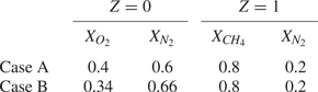
The fuel jet is composed of methane and nitrogen, whereas the oxidizer coflow consists of oxidizer and nitrogen. Two cases, i.e. case A and case B, with different fuel and oxidizer composition are simulated. The values of the composition for the two cases are provided in table 1. The two cases feature different levels of flame extinction and different behaviours of flame edges as will be examined later in the paper.
Stream compositions of the simulations.

The mean inflow velocity and mixture fraction profiles are based on hyperbolic tangent functions. Here, the mixture fraction,  $Z$, is based on the Bilger's definition (Bilger Reference Bilger1976). The inlet profiles of mean flow velocity magnitude
 $\bar {u}$ and mean mixture fraction
 $\bar {Z}$ are described as
 \begin{gather} {\bar{u}(y)}=U_j+\dfrac{U_c-U_j}{2}\left(1+{\tanh \left(\dfrac{(y-y_0)\cos\theta-H/2}{\delta_u}\right)} {\tanh \left(\dfrac{(y-y_0)\cos\theta + H/2}{\delta_u}\right)}\right), \end{gather}
 \begin{gather} \bar{Z}(y)=\dfrac{1}{2}\left(1-{\tanh\left(\dfrac{(y-y_0)\cos\theta-H_Z/2}{\delta_Z}\right)} {\tanh\left(\dfrac{(y-y_0)\cos\theta+H_Z/2}{\delta_Z}\right)}\right), \end{gather}
where  $\theta$ is the angle between the jet to the wall at the inlet,
 $\delta _u$ is the initial shear layer thickness with
 $\delta _u=H/15$ and
 $\delta _Z$ is the initial thickness of mixture fraction variation with
 $\delta _Z=H_Z/5$. Both the jet and coflow velocities have two components that are non-zero at the inlet, i.e. one in the
 $x$ direction and the other in the
 $y$ direction.
The effects of radiative heat transfer are ignored to simplify the physical problem and to focus on the flame edge dynamics. Note that this simplification may over-estimate the flame temperature and lead to lower levels of flame extinction (Chao, Law & T'ien Reference Chao, Law and T'ien1991). Although viewed as a questionable simplification, radiative heat transfer is neglected in the present work. The radiation effects will be investigated in our future work. The wall temperature  $T_w$ is constant during the simulations and its value is 573 K. The initial temperature for the jet is
 $T_j = 700\ \textrm {K}$, and that for the coflow is
 $T_c = 573\ \textrm {K}$, the same as
 $T_w$. A chemically inert wall boundary condition is considered. Note that surface reactions in conditions of high radical concentration very close to the wall at high temperatures may facilitate the adsorption/desorption processes on the wall and influence the flame behaviours (Vlachos, Schmidt & Aris Reference Vlachos, Schmidt and Aris1994; Popp & Baum Reference Popp and Baum1997). Recently, Narukawa et al. (Reference Narukawa, Minamoto, Shimura and Tanahashi2020) showed that surface reactions are limited to the wall surface and have a small effect on flame quantities such as propagation speeds. In the present work, the radical concentrations very close to the wall are low (Wang et al. Reference Wang, Chen, Luo, Hawkes, Chen and Fan2021a), and the flame edges should not be influenced much by surface reactions. Therefore, the contribution of surface reactions is expected to be minor, and it is not included in the DNS.
The simulations are initialized by laminar flamelet solutions, which are generated by FlameMaster (Pitsch Reference Pitsch1998). The stoichiometric scalar dissipation rate  $\chi _{st}$ of the flamelets is
 $0.7\chi _q$, where
 $\chi _q$ is the extinction scalar dissipation rate. The values of
 $\chi _q$ are
 $2300\ \textrm {s}^{-1}$ and
 $1220\ \textrm {s}^{-1}$ for cases A and B, respectively. The scalar dissipation rate
 $\chi$ is calculated as
 $\chi =2D|{\nabla } Z|^2$, where
 $D$ is the thermal diffusivity. The Damköhler number (
 $Da$) which measures the interactions of flame and large-scale turbulence is given as
 $Da=\chi _q \tau _j$, where
 $\tau _j$ is the flow time scale estimated as
 $\tau _j=H/\Delta {U}$. The values of
 $Da$ are 0.021 and 0.011 for cases A and B, respectively. Therefore, case A is expected to be more resilient to extinction than case B.
The jet turbulence is triggered by superimposing isotropic turbulent fluctuations on the inlet profile of the mean velocity, which are filtered outside of the jet. The isotropic velocity field is generated based on a kinetic energy spectrum function by Passot & Pouquet (Reference Passot and Pouquet1987). The inlet turbulent velocity,  $u'$, is 0.1
 $U_j$. The inlet turbulent integral length scale,
 $l_t$, is equal to the jet width
 $H$. Note that although the jet turbulence, which is away from the wall, develops quickly in the free shear region, the boundary layer turbulence has not developed yet. The near-wall turbulence is mainly characterized by the interactions of jet turbulence and the wall, and the structure of the near-wall turbulence differs from typical boundary layer turbulence characterized by hairpin vortex (Wang et al. Reference Wang, Wang, Luo, Hawkes, Chen and Fan2021c). This also has an effect on the choice of resolution for the DNS near the wall, which is explained in the following.
The domain size of the DNS cases is  $L_{x}=42H$ in the streamwise direction (
 $x$),
 $L_{y}=16H$ in the wall-normal direction (
 $y$) and
 $L_{z}=8H$ in the spanwise direction (
 $z$). The boundary conditions are non-reflecting in the
 $x$ direction and periodic in the
 $z$ direction. The boundary condition is no-slip isothermal wall at
 $y=0$ and non-reflecting outflow at
 $y=L_y$. Uniform grids are used in the
 $x$ and
 $z$ directions with
 $\Delta {x} = \Delta {z} = 29 \ \mathrm {\mu } \textrm {m}$. The grid in the
 $y$ direction is uniform with
 $\Delta {y} = 15 \ \mathrm {\mu } \textrm {m}$ when
 $y \le 4.2\ \textrm {mm}$, and gradually stretched outside of this region with a maximum relative stretch rate of 1.0 %. The stretch function is similar to that in Hawkes et al. (Reference Hawkes, Chatakonda, Kolla, Kerstein and Chen2012). There is at least 0.6 grid for the Kolmogorov scale
 ${\eta }$ in the whole domain for solving turbulence and more than 10 grids for solving flame structures, i.e.
 $\Delta {y}/\eta < {0.6}$. The Kolmogorov scale is estimated locally as
 $\eta = (\nu ^3/\epsilon )^{1/4}$, where
 $\nu$ is the viscosity and
 $\epsilon$ is the kinetic energy dissipation rate. In the present DNS, the resolution of turbulence in the free shear region is more demanding, where the Kolmogorov scale has the lowest values. In the near-wall region, boundary layer turbulence is not developed yet, and turbulence near the wall of the present DNS appears just due to the interactions between jet turbulence and the wall, which is well resolved using the DNS grids. For both cases, the grid number is
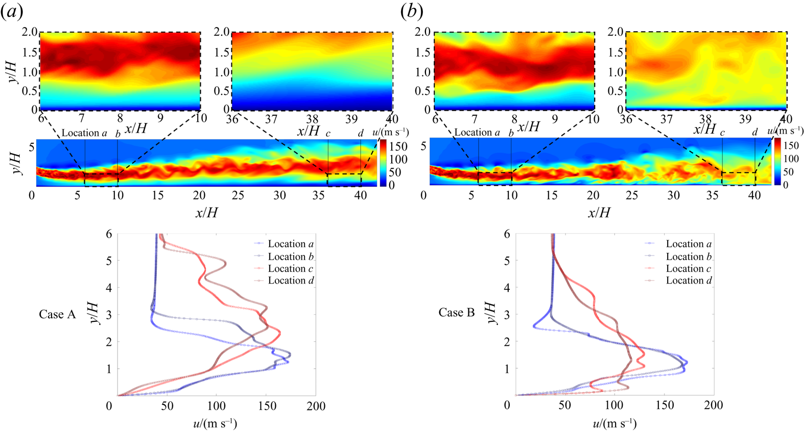
 $N_{x} \times N_{y} \times N_{z} = 1560 \times 560 \times 300$. To further verified the resolution in the near-wall region where the grids are demanding, the streamwise velocity contour in typical
 $x - y$ planes and the streamwise velocity profiles in the wall-normal direction at several representative locations for both cases are shown in figure 2. The DNS grids are also superimposed on the velocity profiles. It is clearly observed that the resolution is sufficient to resolve the large velocity gradient near the wall.
The streamwise velocity contour in typical  $x - y$ planes and the streamwise velocity profiles in the wall-normal direction at several representative locations for (a) case A and (b) case B. The DNS grids are also superimposed on the velocity profiles.

2.2. Numerical methods
The DNS code S3D is employed to solve the Navier–Stokes equations for compressible reacting flows (Chen et al. Reference Chen2009). A six-stage fourth-order explicit Runge–Kutta method and an eighth-order central differencing scheme are used for time integration and spatial derivatives, respectively (Kennedy & Carpenter Reference Kennedy and Carpenter1994; Kennedy, Carpenter & Lewis Reference Kennedy, Carpenter and Lewis2000). High-frequency oscillations are diminished by using a tenth-order filter (Kennedy & Carpenter Reference Kennedy and Carpenter1994).
The DNS used a 17 species and 73-step mechanism for methane combustion, among which four species (CH $_2$, CH
 $_2$(s), HCO and CH
 $_2$OH) are identified as quasi-steady-state species. The mechanism was validated in a steady counter-flow flame with CHEMKIN (Kee, Rupley & Miller Reference Kee, Rupley and Miller1989) by comparing the predictions from several mechanisms with different levels of complexity (Wang et al. Reference Wang, Chen, Luo, Hawkes, Chen and Fan2021a). The DNS advanced for more than 3
 $t_f$ after the flame achieved a statistically steady state to collect stationary statistics, where
 $t_f$ is the flow through time defined as
 $t_f = L_x/\Delta {U}$.
2.3. Characterization of flame edges
2.3.1. Flame edge detection
The flame edge is the line defined as the intersection of  $\phi =\phi ^*$ and
 $Z=Z_{st}$ iso-surfaces, where
 $\phi$ is a scalar for measuring the reaction progress,
 $\phi ^*$ is its critical value and
 $Z_{st}$ is the stoichiometric mixture fraction. The scalar
 $\phi$ can be a product mass fraction, a radical species mass fraction, or temperature. Here, we use the mass fraction of hydroxyl radical
 $Y_{OH}$ as the scalar to characterize flame edges. The critical value of hydroxyl radical
 $Y^*_{OH}$ is defined as 10 % of the global maximum value of
 $Y_{OH}$. The choice of the critical value has been discussed in Wang et al. (Reference Wang, Chen, Luo, Hawkes, Chen and Fan2021a). In order to extract the flame edges, a parallel implementation of the marching cubes algorithm was applied to triangulate the stoichiometric mixture fraction iso-surface, and then the flame edges were linearly interpolated based on the vertex where
 $Y_{OH}=Y^*_{OH}$.
2.3.2. Flame edge coordinates
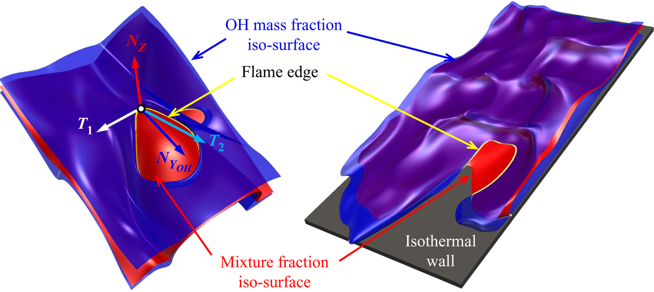
As shown in figure 3, the vector  $\boldsymbol {N}_Z$ represents the unit vector normal to the mixture fraction iso-surface pointing towards the oxidizer stream, which is defined as
 \begin{equation} \boldsymbol{N}_Z={-}\frac{\boldsymbol{\nabla} Z}{|\boldsymbol{\nabla} Z|}. \end{equation}
Schematics of canonical flame edge (left) and flame edge near the wall (right).

Similarly,  $\boldsymbol {N}_{OH}$ is the unit vector normal to the
 $Y_{OH}$ iso-surface pointing towards low values of
 $Y_{OH}$ defined as
 \begin{equation} \boldsymbol{N}_{Y_{OH}}={-}\frac{\boldsymbol{\nabla} Y_{OH}}{|\boldsymbol{\nabla} Y_{OH}|}. \end{equation}
The unit vector  $\boldsymbol {T}_1$ is normal to both
 $\boldsymbol {N}_Z$ and
 $\boldsymbol {N}_{Y_{OH}}$, and the unit vector
 $\boldsymbol {T}_2$ is normal to both
 $\boldsymbol {T}_1$ and
 $\boldsymbol {N}_Z$. These vectors are given by
 \begin{gather} \boldsymbol{T}_1=\frac{\boldsymbol{N}_{Y_{OH}} \times \boldsymbol{N}_Z}{|\boldsymbol{N}_{Y_{OH}} \times \boldsymbol{N}_Z|}, \end{gather}
 \begin{gather} \boldsymbol{T}_2=\frac{\boldsymbol{N}_Z \times (\boldsymbol{N}_{Y_{OH}} \times \boldsymbol{N}_Z)}{|\boldsymbol{N}_{Y_{OH}} \times \boldsymbol{N}_Z|}. \end{gather}
The numerator of  $\boldsymbol {T}_2$ can be expanded using Lagrange's formula as
 \begin{gather} \boldsymbol{N}_Z \times (\boldsymbol{N}_{Y_{OH}} \times \boldsymbol{N}_Z)=\boldsymbol{N}_{Y_{OH}}(\boldsymbol{N}_Z \boldsymbol{\cdot} \boldsymbol{N}_Z) - \boldsymbol{N}_Z(\boldsymbol{N}_{Y_{OH}} \boldsymbol{\cdot} \boldsymbol{N}_Z)=\boldsymbol{N}_{Y_{OH}} -\boldsymbol{N}_Z(\boldsymbol{N}_{Y_{OH}} \boldsymbol{\cdot}\boldsymbol{N}_Z), \end{gather}
whereas the denominator of  $\boldsymbol {T}_2$ is rewritten as
 \begin{equation} |\boldsymbol{N}_{Y_{OH}} \times \boldsymbol{N}_Z|=|\boldsymbol{N}_Z||\boldsymbol{N}_{Y_{OH}}| \sqrt{1-(\boldsymbol{N}_{Y_{OH}} \boldsymbol{\cdot} \boldsymbol{N}_Z)^2}= \sqrt{1-(\boldsymbol{N}_{Y_{OH}} \boldsymbol{\cdot} \boldsymbol{N}_Z)^2}. \end{equation}
Therefore,  $\boldsymbol {T}_2$ can be rewritten as
 \begin{equation} \boldsymbol{T}_2 = \frac{\boldsymbol{N}_{Y_{OH}} - \boldsymbol{N}_Z(\boldsymbol{N}_{Y_{OH}} \boldsymbol{\cdot} \boldsymbol{N}_Z)} {\sqrt{1-(\boldsymbol{N}_{Y_{OH}} \boldsymbol{\cdot} \boldsymbol{N}_Z)^2}}. \end{equation}
2.3.3. Flame edge speed
The displacement speed of mixture fraction and OH mass fraction is given as (Echekki & Chen Reference Echekki and Chen1998; Im & Chen Reference Im and Chen1999, Reference Im and Chen2001; Pantano Reference Pantano2004)
 \begin{gather} S_Z={-}\frac{1}{\rho |\boldsymbol{\nabla} Z|}\left(\frac{\partial}{\partial x_j}\left(\rho D \frac{\partial Z}{\partial x_j}\right)\right), \end{gather}
 \begin{gather} S_d={-}\frac{1}{\rho |\boldsymbol{\nabla} Y_{OH}|}\left(\dot\omega_{Y_{OH}}+\frac{\partial}{\partial x_j}\left(\rho D_{OH} \frac{\partial Y_{OH}}{\partial x_j}\right)\right), \end{gather}
respectively, where  $D$ and
 $D_{OH}$ are diffusivities of mixture fraction and OH radical, respectively.
The flame edge speed  $S_e$ is the projection of overall displacement velocity of the flame edge
 $\boldsymbol {V}_e$ on the iso-surface of
 $Z_{st}$:
 \begin{equation} S_e=\boldsymbol{V}_e \boldsymbol{\cdot} \boldsymbol{T}_2. \end{equation}
Combining (2.9) and (2.12),  $S_e$ is written as
 \begin{equation} S_e = \frac{ \boldsymbol{V}_e \boldsymbol{\cdot} \boldsymbol{N}_{Y_{OH}} + \boldsymbol{V}_e \boldsymbol{\cdot} \boldsymbol{N}_Z (\boldsymbol{N}_{Y_{OH}} \boldsymbol{\cdot} \boldsymbol{N}_Z)} {\sqrt{1-(\boldsymbol{N}_{Y_{OH}} \boldsymbol{\cdot} \boldsymbol{N}_Z)^2}} = \frac{S_d-kS_Z}{\sqrt{1-k^2},} \end{equation}
where  $k=\boldsymbol {N}_{Y_{OH}} \boldsymbol {\cdot } \boldsymbol {N}_Z$ (note that
 $\boldsymbol {V}_e \boldsymbol {\cdot } \boldsymbol {N}_Z = S_Z$ and
 $\boldsymbol {V}_e \boldsymbol {\cdot } \boldsymbol {N}_{Y_{OH}} = S_d$).
The displacement speed of OH mass fraction iso-surface in (2.11) can be decomposed into three components as follows (Chakraborty & Mastorakos Reference Chakraborty and Mastorakos2006; Hesse, Chakraborty & Mastorakos Reference Hesse, Chakraborty and Mastorakos2009; Wang, Hawkes & Chen Reference Wang, Hawkes and Chen2017a; Wang et al. Reference Wang, Hawkes, Chen, Zhou, Li and Aldén2017b):
 \begin{equation} S_d = S_{d,n} + S_{d,t} + S_{d,r}, \end{equation}
where  $S_{d,n}$,
 $S_{d,t}$ and
 $S_{d,r}$ are the normal diffusion, tangential diffusion and reaction components of
 $S_d$, respectively,
 \begin{gather} S_{d,n} ={-}\frac{\boldsymbol{N}_{Y_{OH}} \boldsymbol{\cdot} \boldsymbol{\nabla} (\rho D \boldsymbol{N}_{Y_{OH}}\boldsymbol{\cdot} \boldsymbol{\nabla} Y_{OH})}{\rho |\boldsymbol{\nabla} Y_{OH}|}, \end{gather}
 \begin{gather} S_{d,t} = D\kappa_{Y_{OH}}, \end{gather}
 \begin{gather} S_{d,r} ={-}\frac{\dot\omega_{Y_{OH}}}{\rho |\boldsymbol{\nabla} Y_{OH}|} , \end{gather}
where  $\kappa _{Y_{OH}}$ is the curvature of the OH mass fraction iso-surface defined as
 $\boldsymbol {\nabla } \boldsymbol {\cdot } \boldsymbol {N}_{Y_{OH}}$. Similarly, the displacement speed of stoichiometric mixture fraction iso-surface in (2.10) can be decomposed into two components as
 \begin{gather} S_{Z,n} ={-}\frac{\boldsymbol{N}_Z \boldsymbol{\cdot} \boldsymbol{\nabla} (\rho D \boldsymbol{N}_Z\boldsymbol{\cdot} \boldsymbol{\nabla} Z)}{\rho |\boldsymbol{\nabla} Z|}, \end{gather}
 \begin{gather} S_{Z,t} = D\kappa_Z, \end{gather}
where  $\kappa _Z$ is the curvature of the stoichiometric mixture fraction iso-surface defined as
 $\boldsymbol {\nabla } \boldsymbol {\cdot } \boldsymbol {N}_Z$.
The flame edge speed is weighted by density to account for the thermal expansion effects across the flame as
 \begin{equation} S_e^*/S_L=\frac{\rho S_e}{\rho_u S_L}, \end{equation}
where  $\rho _u$ is the unburnt gas density and
 $S_L$ is the reference laminar flame speed. The values of unburnt gas density and reference laminar flame speed are based on the stoichiometric condition obtained from adiabatic mixing of the oxidizer and fuel streams.
3. Results and discussion
In this section, the general characteristics of the burning/quenching scenarios in the impinging slot-jet flames are first examined. Then, the flame edge structures and dynamics are explored in various regions of the flames. Finally, the effects of wall on flame edges and the interactions between flame edges and turbulence in the near-wall region are reported.
3.1. General characteristics
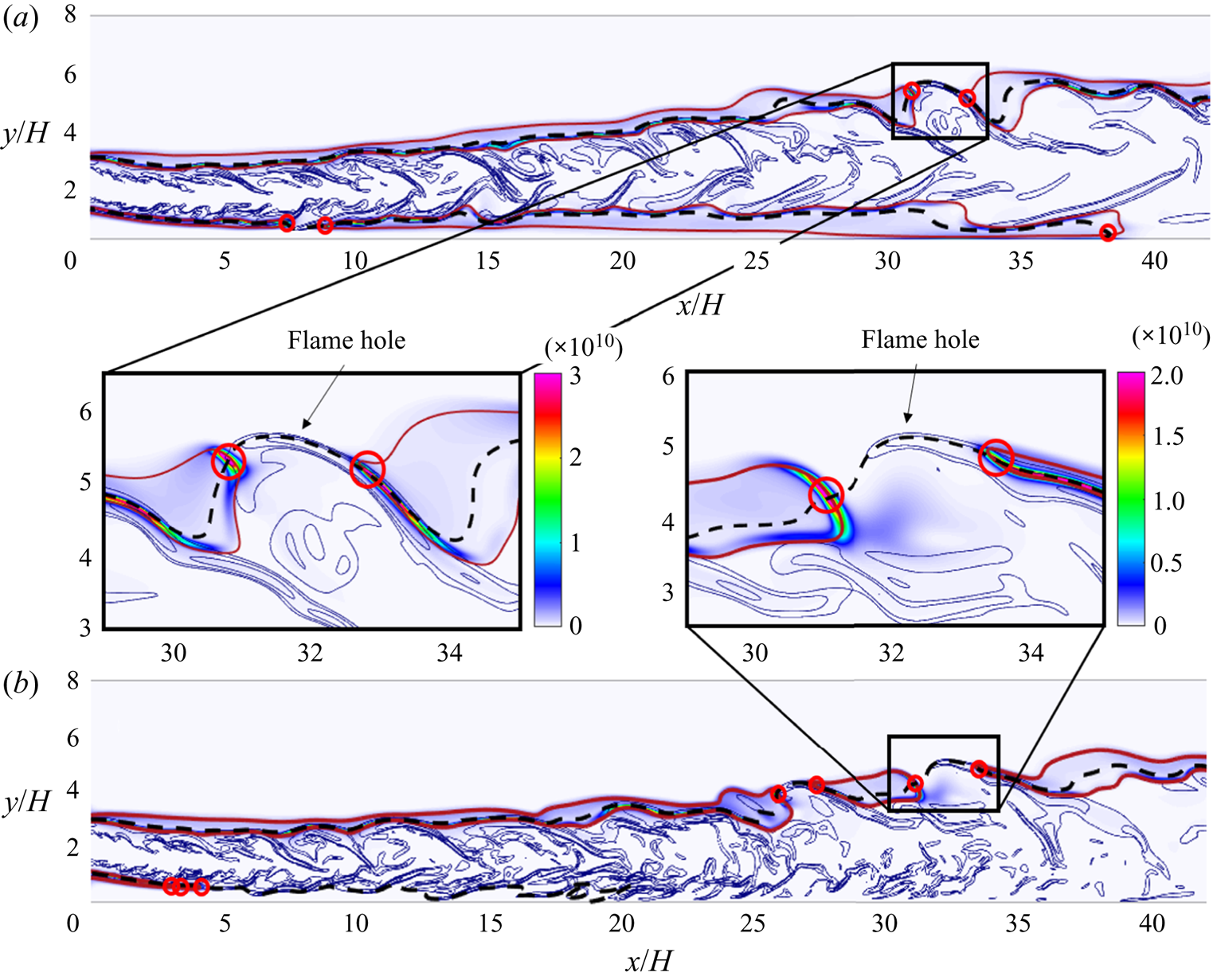
Figure 4 shows instantaneous distributions of heat release rate and scalar dissipation rate in a typical  $x - y$ plane for cases A and B. The red solid lines and black dashed lines indicate the iso-lines of
 $Y^*_{OH}$ and
 $Z_{st}$, respectively. The flame edges are highlighted in red circles. The quenching regions are shown in the inserts of figure 4. As can be seen, there are two flame branches for both cases, including an upper branch and a lower branch. Extinction happens in both cases, and flame quenching is more notable in case B than case A. In particular, for the upper branch of the flames, there are fewer flame holes in case A than in case B. For the lower branch of case A, local extinction occurs in the inclined region. Following that, burning continues along the
 $Z_{st}$ iso-surface and the flame quenches totally near the wall in the downstream region where the oxidizer is consumed completely. In contrast, for the lower branch of case B, the flame is extinguished totally in the inclined region where fuel and oxidizer are still available. More details of flame quenching statistics can be found in our previous work (Wang et al. Reference Wang, Chen, Luo, Hawkes, Chen and Fan2021a).
Instantaneous distributions of heat release rate ( $\textrm {J}\,\textrm {m}^{-3}\,\textrm {s}^{-1}$) at
 $t=247.5 \tau _j$ in a typical
 $x - y$ plane: (a) case A and (b) case B. Both contours are superimposed with stoichiometric mixture fraction (black dashed lines),
 $Y_{OH}=Y^*_{OH}$ (red solid lines) and scalar dissipation rate (thin blue solid lines). The identified flame edges are marked as the centres of the red circles.

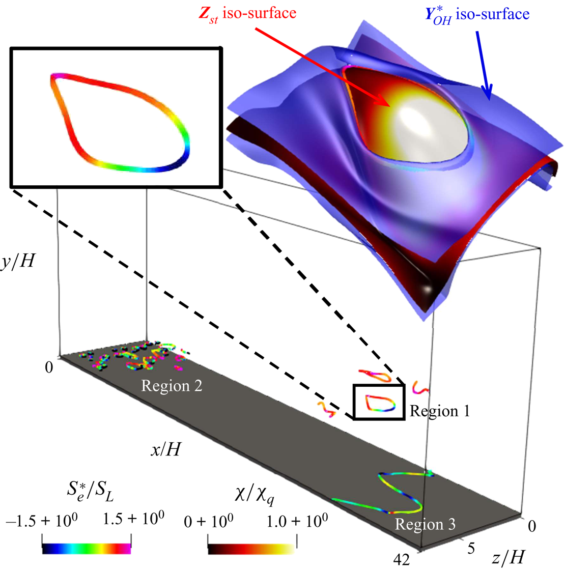
Figure 5 illustrates the instantaneous positions of flame edges coloured by  $S_e^*/S_L$ of case A. Three regions marked as regions 1, 2, and 3 are identified, where region 1 represents the downstream region of the upper flame branch and regions 2 and 3 indicate the upstream and downstream regions of the lower flame branch, respectively. Several observations can be made. First, the flame edges appear as enclosed curves in regions 1 and 2 and as open curves in region 3. Second, as can be seen in the top left of the figure, the propagation speed of flame edges is positive (negative) in upstream (downstream) of the flame hole. Finally, the scalar dissipation is much larger in the downstream regions of the flame hole, indicating that
 $S_e$ and
 $\chi$ are negatively correlated. Such a negative correlation of
 $S_e$ with
 $\chi$ will be further investigated in the next section. A similar figure can also be made for case B. However, only regions 1 and 2 can be identified. Region 3 disappears as the lower flame branch of case B totally extinguishes in the upstream region.
Instantaneous distributions of flame edges of case A. The top left shows the curves of flame edges coloured by  $S_e^*/S_L$ and the top right shows the mixture fraction iso-surface coloured by
 $\chi /\chi _q$ and OH mass fraction iso-surface coloured in blue.

3.2. Flame edge dynamics
Flame edges can retreat due to turbulence or heat loss (Chung Reference Chung2007), resulting in the growth of the flame hole. In contrast, flame edges with a positive propagation speed facilitate flame holes to heal. As the flame edge dynamics represent one of the most significant issues for turbulent non-premixed flames (Dold Reference Dold1989; Hartley & Dold Reference Hartley and Dold1991; Domingo & Vervisch Reference Domingo and Vervisch1996), in the following we investigate the structures of flame edges and explore the effects of scalar dissipation rate on flame edge dynamics.
Figure 6 shows the slices of logarithmic normalized scalar dissipation rate (6a), and normalized heat release rate (6b) in region 1 of case A, where the vorticity magnitude is also superimposed. As can be seen, the values of  $\chi$ at the downstream point of the flame edges around a flame hole are larger than those at the upstream point. The structures of upstream and downstream flame edges are tribrachial and monobrachial, respectively. Note that figure 5 shows the speed of upstream and downstream flame edges is positive and negative, respectively. Similar observations were made in previous experimental studies (Ko, Chung & Chung Reference Ko, Chung and Chung2002; Kim et al. Reference Kim, Seo, Oh and Shin2005), which found that a tribrachial flame edge is related to a positive propagation speed, whereas a monobrachial flame edge is characterized by a negative propagation speed.
Slices of (a) scalar dissipation rate and (b) heat release rate in region 1 of case A. Flame edges are marked with yellow circles. Both contours are superimposed with vorticity magnitude (thin black solid lines).

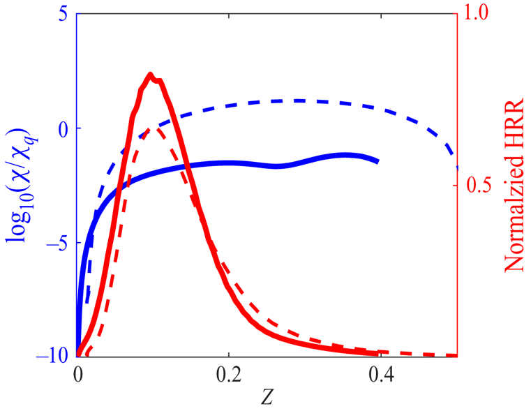
To further investigate the structures of flame edges, two lines, i.e. lines A and B, are identified in figure 6, which are perpendicular to the iso-lines of  $Z_{st}$. Figure 7 displays the profiles of
 $\log _{10}(\chi /\chi _q)$ and normalized heat release rate along the two lines as a function of mixture fraction. As can be seen, for both lines,
 $\log _{10}(\chi /\chi _q)$ increases as
 $Z$ increases. At the stoichiometric mixture fraction (
 $Z_{st}=0.1345$),
 $\chi$ is larger than
 $\chi _q$ for line B. On the other hand, the value of
 $\chi$ is always less than
 $\chi _q$ for line A. The value of the normalized heat release of point A is larger than that of point B. These are consistent with the observations of figure 5.
The profiles of scalar dissipation rate and heat release rate as a function of mixture fraction (line A, solid lines; line B, dashed lines). The heat release rate is normalized by its maximum value in the DNS.

The normal vectors of the  $Y^*_{OH}$ and
 $Z_{st}$ iso-lines,
 $\boldsymbol {N}_{Y_{OH}}$ and
 $\boldsymbol {N}_Z$, are marked on the flame edges in figure 6. As can be seen,
 $\boldsymbol {N}_{Y_{OH}}$ and
 $\boldsymbol {N}_Z$ are perpendicular and anti-aligned for the upstream and downstream of the flame edges, respectively. In general, the inner product of
 $\boldsymbol {N}_{Y_{OH}}$ and
 $\boldsymbol {N}_Z$, i.e.
 $k$, is expected to be zero under laminar or weakly turbulent conditions. For the downstream point B, owing to the effects of strong turbulent mixing,
 $\boldsymbol {N}_{Y_{OH}}$ and
 $\boldsymbol {N}_Z$ are anti-aligned. A similar observation was made by Karami et al. (Reference Karami, Hawkes, Talei and Chen2016). The joint probability density function (p.d.f.) of
 $k$ and logarithmic normalized scalar dissipation rate
 $\log _{10}(\chi /\chi _q)$ in region 1 for case A is shown in figure 8. The black dashed line indicates the conditional means of
 $k$. It is obvious that the value of
 $k$ is less than zero overall, and
 $k$ is negatively correlated with
 $\log _{10}(\chi /\chi _q)$. For low
 $\chi$, the value of
 $k$ is close to zero; whereas for high
 $\chi$, the value of
 $k$ approaches
 $-$1. Such a correlation of
 $\chi$ and
 $k$ confirms the discussion of figure 6, i.e. the anti-alignment behaviour of
 $\boldsymbol {N}_{Y_{OH}}$ and
 $\boldsymbol {N}_Z$ is more evident with increasing
 $\chi$.
Joint p.d.f. and conditional means (dashed line) of  $k$ and logarithmic normalized scalar dissipation rate in region 1 for case A.

The flame edge speed is an important quantity in flame edge dynamics. In order to show the effects of turbulent mixing on flame edge speed, the joint p.d.f.s of  $S_e^*/S_L$ and
 $\log _{10}(\chi /\chi _q)$ in various regions of cases A and B are examined in figure 9. The conditional means of
 $S_e^*/S_L$ are shown in black dashed lines. It is obvious that
 $S_e^*/S_L$ and
 $\log _{10}(\chi /\chi _q)$ are negatively correlated in various regions, except in region 3 of case A. In particular, in figure 9(a,b,d),
 $S_e^*/S_L$ decreases slowly with increasing
 $\log _{10}(\chi /\chi _q)$ at low
 $\chi$ conditions. When
 $\log _{10}(\chi /\chi _q)>0$,
 $S_e^*/S_L$ decreases evidently, and negative values of
 $S_e^*/S_L$ are prevalent, which is consistent with the phenomenon of flame edge retreating and flame holes expansion in high scalar dissipation rate conditions (Pantano & Pullin Reference Pantano and Pullin2004). In figure 9(e), the flame edge speed is mostly negative. The large negative flame edge speed in region 2 of case B is also consistent with the total extinction observed for the lower branch of case B.
Joint p.d.f.s and conditional means (dashed lines) of  $S_e^*/S_L$ and logarithmic normalized scalar dissipation rate.

In regions 1 and 2 of both case A and case B, the motions of flame edges are predominantly affected by turbulent mixing. In contrast, figure 9(c) shows  $S_e^*/S_L$ is rarely correlated with
 $\log _{10}(\chi /\chi _q)$ in region 3 of case A, which is positioned in the near-wall region. It is noted that the values of
 $\log _{10}(\chi /\chi _q)$ in region 3 are much lower than those in regions 1 and 2 of case A. The results indicate that the value of
 $\chi$ is so small that the motion of flame edges is not sensitive to
 $\chi$ near the wall. The factors that influence flame edge dynamics near the wall will be explored in the next section.
It is also seen that  $S_e^*$ is of the same order as
 $S_L$ in the present work, which contrasts some previous experimental studies showing large values of flame edge speed (Hasselbrink & Mungal Reference Hasselbrink and Mungal1998; Steinberg et al. Reference Steinberg, Boxx, Arndt, Frank and Meier2011; Juddoo & Masri Reference Juddoo and Masri2011). Note that the gas at the location of extinction in the flames is not pure fuel and oxidizer, but a partially reacted mixture. A density-weighted speed of flame edges is used to account for this effect in this paper (see (2.20)), which may explain the lower values of flame edge speed in the present work compared with the previous experiments. This treatment is similar to other DNS studies (Sripakagorn et al. Reference Sripakagorn, Mitarai, Kosaly and Pitsch2004; Wang, Hawkes & Chen Reference Wang, Hawkes and Chen2011; Karami et al. Reference Karami, Hawkes, Talei and Chen2015), and consistent results of flame edge speed are obtained in these studies.
3.3. The wall effects on flame edges
3.3.1. Combustion modes
There are two combustion modes, i.e. premixed and non-premixed. The flame index (FI) was first proposed by Yamashita, Shimada & Takeno (Reference Yamashita, Shimada and Takeno1996) and the normalized flame index (NFI) is used in this study:
 \begin{equation} \textrm{NFI} = \boldsymbol{N}_{Y_{F}} \boldsymbol{\cdot} \boldsymbol{N}_{Y_{O}}=\frac{\boldsymbol{\nabla} Y_F \boldsymbol{\cdot} \boldsymbol{\nabla} Y_O}{|\boldsymbol{\nabla} Y_F| |\boldsymbol{\nabla} Y_O|}, \end{equation}
where the subscripts ‘ $F$’ and ‘
 $O$’ denote fuel and oxidizer, respectively. A positive value of NFI indicates premixed combustion whereas a negative value implies non-premixed combustion.
Figure 10 displays the instantaneous distributions of NFI in a typical  $x - y$ plane of case A. The red solid lines and blue dashed lines indicate the
 $Z_{st}$ and
 $Y^*_{OH}$ iso-lines, respectively. As shown in the left bottom of figure 10, the upstream and downstream points of a flame hole are marked as ‘A’ and ‘B’, respectively. The point on flame edges close to the wall, shown in right bottom of figure 10, is marked as point ‘C’. It is seen that NFI of upstream and downstream points (A and B) of the flame hole are positive and negative, respectively. Therefore, partially premixed combustion occurs at point A. This is consistent with the study of Favier & Vervisch (Reference Favier and Vervisch2001), which showed the existence of a partial premixed zone around the flame hole in non-premixed flames. Figure 11 shows the p.d.f.s of NFI for various regions of flame edges in case A. As can be seen, there are two peaks of NFI for Region 1 and the most probable value of NFI is
 $-1$ for all regions. These results indicate both combustion modes exist in region 1 and non-premixed combustion is dominant in the entire flame as expected.
Instantaneous distributions of NFI in a typical  $x - y$ plane of case A.

The p.d.f.s of NFI for different regions of case A.

3.3.2. Flame edge speed
In flame–wall interactions, two quenching modes are widely encountered, i.e. HOQ and SWQ, according to the angle between the edge flame normal vector  $\boldsymbol {N}_Z$ and wall surface normal vector
 $\boldsymbol {N}_{wall}$. In this study, HOQ (SWQ) is characterized by
 $|\boldsymbol {N}_{Z}\boldsymbol {\cdot }\boldsymbol {N}_{wall}|\ge 0.5$ (
 $|\boldsymbol {N}_{Z}\boldsymbol {\cdot }\boldsymbol {N}_{wall}|<0.5$). Figure 12 shows the p.d.f. of
 $\boldsymbol {N}_{Z}\boldsymbol {\cdot }\boldsymbol {N}_{wall}$ for flame edges near the wall of case A (i.e. region 3 in figure 5). The p.d.f. of
 $\boldsymbol {N}_{Z}\boldsymbol {\cdot }\boldsymbol {N}_{wall}$ has two peaks at
 $\boldsymbol {N}_{Z}\boldsymbol {\cdot }\boldsymbol {N}_{wall}=1$ and
 $-1$, implying HOQ is dominant. There exist two types of HOQ and both are important. Specifically,
 $\boldsymbol {N}_{Z}\boldsymbol {\cdot }\boldsymbol {N}_{wall}=1$ (
 $-1$) indicates the edge flame normal is pointing upward (downward) as displayed in figure 13. Figure 12 also shows the p.d.f. of
 $\boldsymbol {N}_{Y_{OH}}\boldsymbol {\cdot }\boldsymbol {N}_{wall}$ for flame edges near the wall of case A. The most probable value of the p.d.f. is
 $-1$. Note that the iso-surface of
 $Y^*_{OH}$ is largely parallel to the wall in
 $x/H=28 \sim 38$ in the near-wall region (see figure 4), so that
 $\boldsymbol {N}_{Y_{OH}}$ and
 $\boldsymbol {N}_{wall}$ are mostly anti-aligned.
The p.d.f.s of  $\boldsymbol {N}_{Z}\boldsymbol {\cdot }\boldsymbol {N}_{wall}$ and
 $\boldsymbol {N}_{Y_{OH}}\boldsymbol {\cdot }\boldsymbol {N}_{wall}$ for flame edges near the wall of case A.

Schematics of HOQ configurations: (a)  $\boldsymbol {N}_{Z}\boldsymbol {\cdot }\boldsymbol {N}_{wall}\ge 0.5$; (b)
 $\boldsymbol {N}_{Z}\boldsymbol {\cdot }\boldsymbol {N}_{wall}\le -0.5$.

In the following, the effects of  $\boldsymbol {N}_{Z}\boldsymbol {\cdot }\boldsymbol {N}_{wall}$ on the speed of flame edges near the wall are analysed. Figure 14 shows the joint p.d.f. of
 $S_e^*/S_L$ and
 $\boldsymbol {N}_{Z}\boldsymbol {\cdot }\boldsymbol {N}_{wall}$. It is readily seen that
 $S_e^*/S_L$ increases with increasing
 $\boldsymbol {N}_{Z}\boldsymbol {\cdot }\boldsymbol {N}_{wall}$ and
 $S_e^*/S_L$ is negative (positive) when
 $\boldsymbol {N}_{Z}$ misaligns (aligns) with
 $\boldsymbol {N}_{wall}$. It is obvious that the correlation of
 $S_e^*/S_L$ and
 $\boldsymbol {N}_{Z}\boldsymbol {\cdot }\boldsymbol {N}_{wall}$ is much more evident than that of
 $S_e^*/S_L$ and
 $\log _{10}(\chi /\chi _q)$ as seen in figure 9(c). This indicates that, in the near-wall region, the flame edge orientation plays a more important role in flame edge speed than turbulent mixing, which is different from the situation when the flame edges are away from the wall, where turbulent mixing is controlling the flame edge propagation.
Joint p.d.f.s and conditional means (dashed line) of  $S_e^*/S_L$ and
 $\boldsymbol {N}_{Z}\boldsymbol {\cdot }\boldsymbol {N}_{wall}$ for flame edges near the wall of case A.

To further understand the effects of  $\boldsymbol {N}_{Z}\boldsymbol {\cdot }\boldsymbol {N}_{wall}$ on the speed of flame edges, the joint p.d.f.s of flame edge speed components (see (2.13)) and
 $\boldsymbol {N}_{Z}\boldsymbol {\cdot }\boldsymbol {N}_{wall}$ are presented in figure 15. The correlations of
 $1/\sqrt {1-k^2}$ and
 $-k/\sqrt {1-k^2}$ with
 $\boldsymbol {N}_{Z}\boldsymbol {\cdot }\boldsymbol {N}_{wall}$ are shown in figure 15(a,b). Note that
 $k$ and
 $\boldsymbol {N}_{Z}\boldsymbol {\cdot }\boldsymbol {N}_{wall}$ are negatively correlated (figure 16). Therefore,
 $1/\sqrt {1-k^2}$ and
 $-k/\sqrt {1-k^2}$ conditionally averaged on
 $\boldsymbol {N}_{Z}\boldsymbol {\cdot }\boldsymbol {N}_{wall}$ are close to functions of
 $f(x) = 1/\sqrt {1-x^2}$ and
 $f(x) = x/\sqrt {1-x^2}$, respectively. Figure 15(c,d) indicate that the conditional mean of
 $S_d^*/S_L$ is close to zero, whereas
 $S_Z^*/S_L$ is greater than zero generally and decreases with increasing
 $\boldsymbol {N}_{Z}\boldsymbol {\cdot }\boldsymbol {N}_{wall}$. Figure 15(e,f) present the results of the two terms of
 $S_e^*/S_L$, i.e.
 $S_d^*/S_L/\sqrt {1-k^2}$ and
 $-kS_Z^*/S_L/\sqrt {1-k^2}$. As can be seen, the conditional mean of
 $S_d^*/S_L/\sqrt {1-k^2}$ increases with increasing
 $\boldsymbol {N}_{Z}\boldsymbol {\cdot }\boldsymbol {N}_{wall}$ when
 $\boldsymbol {N}_{Z}\boldsymbol {\cdot }\boldsymbol {N}_{wall}\le -0.5$; it approaches zero when
 $\boldsymbol {N}_{Z}\boldsymbol {\cdot }\boldsymbol {N}_{wall}>-0.5$, which is due to the near-zero value of
 $S_d^*/S_L$. In general, a positive correlation of
 $-kS_Z^*/S_L/\sqrt {1-k^2}$ with
 $\boldsymbol {N}_{Z}\boldsymbol {\cdot }\boldsymbol {N}_{wall}$ is observed, and
 $-kS_Z^*/S_L/\sqrt {1-k^2}$ varies from negative to positive values as
 $\boldsymbol {N}_{Z}\boldsymbol {\cdot }\boldsymbol {N}_{wall}$ increases. Based on the analysis of figure 15, it is concluded that the variations of
 $S_e^*/S_L$ with
 $\boldsymbol {N}_{Z}\boldsymbol {\cdot }\boldsymbol {N}_{wall}$ are contributed by both
 $S_d^*/S_L/\sqrt {1-k^2}$ and
 $-kS_Z^*/S_L/\sqrt {1-k^2}$ when
 $\boldsymbol {N}_{Z}\boldsymbol {\cdot }\boldsymbol {N}_{wall}\le -0.5$, and
 $-kS_Z^*/S_L/\sqrt {1-k^2}$ dominates
 $S_e^*/S_L$ when
 $\boldsymbol {N}_{Z}\boldsymbol {\cdot }\boldsymbol {N}_{wall}\ge 0.5$.
Joint p.d.f.s and conditional means (dashed lines) of (a)  $1/\sqrt {1-k^2}$, (b)
 $-k/\sqrt {1-k^2}$, (c)
 $S_d^*/S_L$, (d)
 $S_Z^*/S_L$, (e)
 $S_d^*/S_L/\sqrt {1-k^2}$ and (f)
 $-kS_Z^*/S_L/\sqrt {1-k^2}$ and
 $\boldsymbol {N}_{Z}\boldsymbol {\cdot }\boldsymbol {N}_{wall}$ for flame edges near the wall of case A.

Joint p.d.f. and conditional means (dashed line) of  $k$ and
 $\boldsymbol {N}_{Z}\boldsymbol {\cdot }\boldsymbol {N}_{wall}$ for flame edges near the wall of case A.

3.3.3. Alignment statistics
The edge flame normal  $\boldsymbol {N}_{Z}$ is a key parameter that influences the dynamics of flame edges based on the above analysis. In the following, the behaviour of
 $\boldsymbol {N}_{Z}$ in the near-wall region is presented and the interactions between flame edges and turbulence are explored in terms of the alignment between the edge flame normal and the principal strain rates.
The strain rate tensor  $S_{ij}$ is used to characterize the small-scale flow structure, which is defined as
 \begin{equation} S_{ij} = \frac{1}{2} \left(\frac{\partial u_i}{\partial x_j}+\frac{\partial u_j}{\partial x_i} \right). \end{equation}
Three principal eigenvalues of  $S_{ij}$ are
 $\lambda _1$,
 $\lambda _2$ and
 $\lambda _3$ with the convention
 $\lambda _1 \ge \lambda _2 \ge \lambda _3$, which are the solutions of the following characteristic equation:
 \begin{equation} \lambda^3+P\lambda^2+Q\lambda+R=0, \end{equation}
where the invariants  $P$,
 $Q$ and
 $R$ are given as
 \begin{gather} P={-}S_{ii}, \end{gather}
 \begin{gather} Q=\tfrac{1}{2}(P^2-S_{ij}S_{ji}-W_{ij}W_{ji}) \end{gather}
and
 \begin{equation} R=\tfrac{1}{3}({-}P^3+3PQ-S_{ij}S_{jk}S_{ki}-3W_{ij}W_{jk}S_{ki}), \end{equation}
where  $W_{ij}=(\partial u_i /\partial x_j-\partial u_j /\partial x_i)/2$ is the rotation tensor.
 $\boldsymbol {e}_1$,
 $\boldsymbol {e}_2$ and
 $\boldsymbol {e}_3$ are the principal eigenvectors of
 $\lambda _1$,
 $\lambda _2$ and
 $\lambda _3$, respectively.
Figure 17(a–c) show the p.d.f.s of the components of  $\boldsymbol {e}_1$,
 $\boldsymbol {e}_2$ and
 $\boldsymbol {e}_3$, respectively, for flame edges near the wall of case A. It is readily observed that the most probable value of
 $\boldsymbol {e}_{1}$ is
 $(-1/\sqrt {2},-1/\sqrt {2},0)$, indicating the most extensive strain rate orients roughly 225
 $^{\circ }$ to the streamwise direction. The most probable value of
 $\boldsymbol {e}_{2}$ is
 $(0,0,-1)$, implying the intermediate strain rate generally orients with the spanwise direction. The most probable value of
 $\boldsymbol {e}_{3}$ is
 $(-1/\sqrt {2},1/\sqrt {2},0)$, denoting the most compressive strain rate orients 135
 $^{\circ }$ to the streamwise direction. For a better illustration of the principal strain rates near the wall, a schematic of
 $\boldsymbol {e}_1$ and
 $\boldsymbol {e}_3$ are shown in a typical
 $x - y$ plane of figure 18 (
 $\boldsymbol {e}_2$ is vertical to this plane and is not shown).
The p.d.f.s of the components of  $\boldsymbol {e}_j$ for flame edges near the wall of case A.

Orientations of  $\boldsymbol {e}_1$ and
 $\boldsymbol {e}_3$ near the wall of case A. Iso-surfaces of
 $\lambda _2=23\,000\,\textrm {s}^1$ (grey),
 $Z_{st}$ (red) and
 $Y_{OH}^*$ (blue) are also shown.

Next, the orientations of  $\boldsymbol {N}_{Z}$ are examined. In particular, the alignment characteristics between edge flame normals and principal strain rates are presented. Figure 19 shows the p.d.f.s of
 $|\boldsymbol {N}_Z \boldsymbol {\cdot } \boldsymbol {e}_j|$ conditioned on
 $\boldsymbol {N}_{Z}\boldsymbol {\cdot }\boldsymbol {N}_{wall}$ for flame edges near the wall of case A. It is interesting to find that the edge flame normal preferentially aligns with the most extensive, intermediate and most compressive strain rates when
 $\boldsymbol {N}_{Z}\boldsymbol {\cdot }\boldsymbol {N}_{wall}\le -0.5$,
 $-0.5<\boldsymbol {N}_{Z}\boldsymbol {\cdot }\boldsymbol {N}_{wall}<0.5$ and
 $\boldsymbol {N}_{Z}\boldsymbol {\cdot }\boldsymbol {N}_{wall}\ge 0.5$, respectively. Previous investigations (Swaminathan & Grout Reference Swaminathan and Grout2006; Chakraborty & Swaminathan Reference Chakraborty and Swaminathan2007; Hartung et al. Reference Hartung, Hult, Kaminski, Rogerson and Swaminathan2008) showed that, when dilatation induced by heat release rate dominates over the turbulent strain, the edge flame normal preferentially aligns with the most extensive strain rate. Therefore, in the following we examine the variation of the dilatation rate with
 $\boldsymbol {N}_{Z}\boldsymbol {\cdot }\boldsymbol {N}_{wall}$ for flame edges near the wall of case A in order to understand the preferential alignments between
 $\boldsymbol {N}_{Z}$ and
 $\boldsymbol {e}_{j}$ conditioned on
 $\boldsymbol {N}_{Z}\boldsymbol {\cdot }\boldsymbol {N}_{wall}$.
The p.d.f.s of  $|\boldsymbol {N}_Z \boldsymbol {\cdot } \boldsymbol {e}_j|$ for flame edges near the wall of case A.

Figure 20(a) shows the joint p.d.f.s of the normalized dilatation rate  $\boldsymbol {\nabla } \boldsymbol {\cdot } \boldsymbol {u} \times \delta _L/S_L$ and
 $\boldsymbol {N}_{Z}\boldsymbol {\cdot }\boldsymbol {N}_{wall}$. As can be seen, the mean dilatation rate reaches its peak value when
 $\boldsymbol {N}_{Z}\boldsymbol {\cdot }\boldsymbol {N}_{wall}=-1$, and decreases as
 $\boldsymbol {N}_{Z}\boldsymbol {\cdot }\boldsymbol {N}_{wall}$ increases. It is also noted that, when
 $-0.5<\boldsymbol {N}_{Z}\boldsymbol {\cdot }\boldsymbol {N}_{wall}< 0.5$, the value of
 $\boldsymbol {\nabla } \boldsymbol {\cdot } \boldsymbol {u} \times \delta _L/S_L$ is nearly zero. The dilatation rate becomes negative for
 $\boldsymbol {N}_{Z}\boldsymbol {\cdot }\boldsymbol {N}_{wall}=1$. Note that the dilatation rate is affected by heat release and/or heat loss, with the former acting as a source and the latter acting as a sink. The heat loss can be represented by the normalized wall heat flux corresponding to the flame edges in the near-wall region. Figure 20(b,c) show the means of normalized wall heat flux and heat release rate doubly conditioned on
 $\boldsymbol {\nabla } \boldsymbol {\cdot } \boldsymbol {u} \times \delta _L/S_L$ and
 $\boldsymbol {N}_{Z}\boldsymbol {\cdot }\boldsymbol {N}_{wall}$. The wall heat flux
 $\varPhi$ is defined as
 $\varPhi =-\lambda \,\textrm {d}T/{\textrm {d}y}$, which is normalized by flame power
 $\rho S_L c_p(T_2-T_1)$, where
 $c_p$ is the specific heat capacity. Here
 $T_1$ and
 $T_2$ are temperatures of product and reactant, respectively. The heat release rate is normalized by its maximum value. It is observed that for negative dilatation rate, the normalized wall heat flux is large. When
 $\boldsymbol {N}_{Z}\boldsymbol {\cdot }\boldsymbol {N}_{wall}\le -0.5$, the heat release rate is large, resulting in a net positive dilatation. Therefore, consistent with previous studies of low
 $Ka$ flames, the heat-release-induced dilatation is dominant over turbulent strain and the edge flame normal aligns with the most extensive strain rate. When
 $-0.5<\boldsymbol {N}_{Z}\boldsymbol {\cdot }\boldsymbol {N}_{wall}<0.5$, the heat release rate and dilatation are both reduced, the edge flame normal preferentially aligns with the intermediate strain rate. Finally, when
 $\boldsymbol {N}_{Z}\boldsymbol {\cdot }\boldsymbol {N}_{wall}\ge 0.5$, the heat loss by the cold wall effect is large enough to counteract the heat release by the chemical reactions and turbulent strain is prevalent. This situation is consistent with those of scalars in non-reacting flows or high
 $Ka$ flames, where the scalar gradient/flame normal preferentially aligns with the most compressive strain rate.
(a) Joint p.d.f. and conditional means (dashed line) of normalized dilatation rate ( $\boldsymbol {\nabla } \boldsymbol {\cdot } \boldsymbol {u} \times \delta _L /S_L$) and
 $\boldsymbol {N}_{Z}\boldsymbol {\cdot }\boldsymbol {N}_{wall}$ conditioned near the wall of case A. (b) The normalized wall heat flux and (c) heat release rate conditionally averaged on
 $\boldsymbol {\nabla } \boldsymbol {\cdot } \boldsymbol {u} \times \delta _L /S_L$ and
 $\boldsymbol {N}_{Z}\boldsymbol {\cdot }\boldsymbol {N}_{wall}$ for flame edges near the wall of case A.

4. Conclusions
In the present study, three-dimensional DNS of planar turbulent non-premixed slot-jet flames impinging at a wall have been analysed to understand the structures and dynamics of flame edges. General characteristics of quenching scenarios are explored and it has been found that extinction is more significant in case B than case A. Two flame branches have been identified in planar jet flames. For flame edges in upper branch flames, the flame edge structures change from tribrachial to monobrachial around a flame hole. The flame edge speed generally increases with increasing scalar dissipation rate when the flame edges are away from the wall.
The wall effects on flame edges have been shown. It was found that turbulent mixing is playing a significant role on the speed of flame edges in the shear layer region; the speed of flame edges in the near-wall region is primarily determined by the projection of edge flame normal in the wall-normal direction, i.e.  $\boldsymbol {N}_{Z}\boldsymbol {\cdot }\boldsymbol {N}_{wall}$. The flame edge speed increases with increasing
 $\boldsymbol {N}_{Z}\boldsymbol {\cdot }\boldsymbol {N}_{wall}$. Under the condition of
 $\boldsymbol {N}_{Z}\boldsymbol {\cdot }\boldsymbol {N}_{wall}\le -0.5$, flame edges are retreating with a negative propagation speed.
The alignment between the edge flame normal and principal strain rates near the wall was examined. When  $\boldsymbol {N}_{Z}\boldsymbol {\cdot }\boldsymbol {N}_{wall}\le -0.5$, the edge flame normal aligns with the most extensive strain rate, which is consistent with previous studies of high
 $Da$ or low
 $Ka$ flames. This is due to the fact that the heat-release-induced dilatation is dominant over the turbulent strain. When
 $-0.5<\boldsymbol {N}_{Z}\boldsymbol {\cdot }\boldsymbol {N}_{wall}<0.5$, the edge flame normal is aligned with the intermediate strain rate. When
 $\boldsymbol {N}_{Z}\boldsymbol {\cdot }\boldsymbol {N}_{wall}\ge 0.5$, the wall heat flux overtakes the effect of heat release on dilatation, resulting in the preferential alignment between the edge flame normal and the most compressive strain rate, consistent with previous studies of non-reacting flows or high
 $Ka$ flames.
Overall the DNS results provide insight into the physics of turbulent non-premixed flames interacting with a wall. The complex structures and dynamics of the flame edges are revealed and the interactions between flame edges and turbulence are explored in the non-premixed flames bounded with a wall. The findings improve our understanding of flame edges near the wall.
Funding
This work was supported by Natural Science Foundation of China (Grant Nos. 51836007 and 52022091).
Declaration of interests
The authors report no conflict of interest.