1 Introduction
Large-scale intense vortices are impressive and devastating coherent structures. They intrigue researchers because they have not yet revealed their secrets regarding their formation and evolution. The presence of asymmetric disturbances inside such vortices is a possible intensification mechanism driven by the differential rotation. A set of spiral rainbands, for instance, is frequently observed in most tropical cyclones. The evolutions of the eyewall and rainbands, as well as their mutual interactions, are believed to play an important role in the vortex dynamics and its intensification (Houze et al. Reference Houze, Chen, Lee, Rogers, Moore, Stossmeister, Bell, Cetrone, Zhao and Brodzik2006). According to wave analysis, spiral bands could be partly explained by vorticity wave dynamics (Guinn & Schubert Reference Guinn and Schubert1993; Reasor et al. Reference Reasor, Montgomery, Marks and Gamache2000; Wang Reference Wang2002b ; Chen, Brunet & Yau Reference Chen, Brunet and Yau2003; Corbosiero, Molinari & Aiyyer Reference Corbosiero, Molinari and Aiyyer2006; Judt & Chen Reference Judt and Chen2010).
In geophysical vortices, potential vorticity (PV) wave packets are emitted by PV anomalies generated, for instance, by latent heat release. These waves are stretched by the radial rotational-wind shear into spiral bands and have been recently coined vortex Rossby waves (Montgomery & Kallenbach Reference Montgomery and Kallenbach1997; Chen & Yau Reference Chen and Yau2001). These inwardly spiralling structures are localized areas of deep clouds in the lower and middle atmosphere, providing heavy rains, strong winds and thunderstorms. Like eyewalls, they are associated with local maxima of absolute vorticity, potential vorticity, convection, and upward and sometimes rotational winds, encountered in the vortex. Some rainbands are likely to evolve into a secondary eyewall (Qiu, Tan & Xiao Reference Qiu, Tan and Xiao2010; Didlake et al. Reference Didlake, Reasor, Rogers and Lee2018); conversely, an eyewall can generate spiral bands (Corbosiero et al. Reference Corbosiero, Molinari and Aiyyer2006).
Wave activity analysis in numerical hurricane-like vortex models shows that vortices only interact with vorticity waves and that the related modes are continuous (Chen et al. Reference Chen, Brunet and Yau2003). Basic-state vortex radial shear increases their radial wavenumbers, which slows down the radial propagation of the wave packets. The latter ceases at the stagnation radius where the radial group velocity vanishes. In the WKB approximation, this radius coincides with the phase-velocity critical radius where the phase angular speed is equal to the basic-vortex rotation frequency (Montgomery & Kallenbach Reference Montgomery and Kallenbach1997; Gao & Zhu Reference Gao and Zhu2016). These waves are thus confined to the near-vortex region and cannot propagate to infinity. They locally exchange kinetic energy and angular momentum with the vortex around the stagnation radius. They can nevertheless transport energy out of the vortex core, whereas wave momentum fluxes can cause an inward transport of angular momentum, intensifying the basic vortex (Montgomery & Enagonio Reference Montgomery and Enagonio1998; Corbosiero et al. Reference Corbosiero, Molinari and Aiyyer2006; Houze et al. Reference Houze, Chen, Lee, Rogers, Moore, Stossmeister, Bell, Cetrone, Zhao and Brodzik2006).
This article focuses on the nonlinear dynamics of continuous vorticity modes embedded in rapidly rotating vortices. Continuous modes are singular and neutral modes related to resonating and propagating waves. The aim of this paper is to make progress in understanding such waves in relation to vortex intensification. In particular, we wish to study wave packet/vortex interactions and the subsequent breaking through the nonlinear critical-layer (CL) theory. The vortical mode singularity is removed by introducing nonlinearity in the CL motion equations, which is relevant to large-Reynolds-number, large-scale atmospheric motions. This theory also sounds relevant for tropical cyclone or tornado intensification because, on the one hand, the nonlinear CL development time scale is faster than the intensification duration yet, on the other hand, this weakly nonlinear approach may give the right order of magnitude for the intensification; it indeed yields a higher intensification than the traditional quadratic order of the non-resonant interaction in numerical simulations that do not resolve the critical layer (Montgomery & Kallenbach Reference Montgomery and Kallenbach1997; Qiu et al. Reference Qiu, Tan and Xiao2010; Caillol Reference Caillol2015). When an asymmetric neutral mode is superimposed on the basic vortex, provided resonance occurs, a first linear stage starts, characterized by the formation of the CL and the beginning of the wave/mean-flow interaction (WMFI). Then, the nonlinear critical layer settles down in a transition stage where the WMFI continues in an unsteady but decelerated way. We assume the existence of a quasi-steady state when the wave packet has become weakly singular; it keeps on interacting with the vortex, but in a slower way, such that perturbation theory may be handled. The emergence of a final quasi-steady state is related to the smoothness of the radial eigenfunction. The weakly singular mode radial structure is indeed sufficiently smooth to enable it to resist shear and store part of the basic-vortex angular momentum, and subsequently to weaken the vortex in this asymptotic stage (Nolan & Farrell Reference Nolan and Farrell1999).
Caillol (Reference Caillol2017) described a slowly space–time evolving asymmetric, singular, helical and vorticity mode in a circular vortex with the same CL theory. This previous paper will be referred to as C17. This amplitude-modulated wave modelled a wave train whose envelope had an
 $O(\unicode[STIX]{x1D716}^{-1})$
vertical extent for a dimensionless wave amplitude
 $\unicode[STIX]{x1D716}$
. He derived the system of evolution equations governing the wave packet amplitude and the wave/vortex interaction-induced mean flow a long time after the interaction started. He observed that the wave packet always broke and noticed that considering a wave packet instead of a single steady mode enhanced the wave/vortex interaction. However, the vortex weakened in the long-time asymptotic stage. We here consider a more compact wave packet. The vertical envelope wavenumber is of order
 $O(\unicode[STIX]{x1D716}^{1/2})$
, and we expect to obtain a faster and stronger interaction in the quasi-steady stage. This regime usually corresponds to a balance between nonlinear effects and the dispersion characterized by a coherent structure (Leibovich Reference Leibovich1970; Kivshar & Malomed Reference Kivshar and Malomed1989; Derzho & Grimshaw Reference Derzho and Grimshaw2002; Shagalov, Reutov & Rybushkina Reference Shagalov, Reutov and Rybushkina2009).
In a cylindrical geometry, the modulated amplitude evolves slowly over height and time. Through the critical-layer coupling, we assume the same space–time scales for the CL-induced mean flow around
 $r_{c}$
. This mean flow cannot be neglected because it is of higher amplitude than the wave packet. Owing to the divergenceless-flow condition, the presence of a mean radial velocity is necessary, which makes the flow asymmetric and even more distorted in the neighbourhood of the CL than in the steady-state assumption. The stagnation line here is no longer axisymmetric but is given by a spiral located near
 $r_{c}$
that slowly varies in height and time in the same way as the wave modulation. To perform the analysis, we use a stressed radius-like coordinate that uniquely parameterizes each streamline (Davis Reference Davis1969; Caillol & Grimshaw Reference Caillol and Grimshaw2004). This variable takes into account the deformed motion that streamlines experience in the neighbourhood of the CL. Streamlines deviate from the critical radius with a spiralling departure proportional to the mean radial velocity. As a result, a secular azimuthal variable naturally arises to describe this spiralling motion. Secularity is required to deal with the CL-induced varying mean flow that thus evolves over the rotational direction as well. The preceding wave packet study in C17 involved a secular time scale, which did not have a true physical sense. In the present study, we argue that the existence of a three-dimensional mean flow coupled with the wave packet strongly affects the nonlinear wave dynamics. In past quasi-steady, three-dimensional CL analytical studies, however, the induced mean flow was not taken into account (Voronovich, Pelinovsky & Shrira Reference Voronovich, Pelinovsky and Shrira1998a
; Voronovich, Shrira & Stepanyants Reference Voronovich, Shrira and Stepanyants1998b
).
We assume that the critical layer forms in the outer vortex core where the mean absolute axial vorticity is smaller than the absolute inertial frequency of the circular vortex, which is relevant to large-scale rapidly rotating vortices (Caillol Reference Caillol2015). A weakly singular vortical mode with an azimuthal wavenumber
 $m$
generates a CL pattern characterized by
 $m$
intersecting helical cylinders winding and spiralling along the vortex axis. These cylinders are three-dimensional separatrices which bound two qualitatively distinct CL flows: the flow outside them spans a
 $2\unicode[STIX]{x03C0}$
azimuthal range whereas the flow inside them spans a
 $2\unicode[STIX]{x03C0}/m$
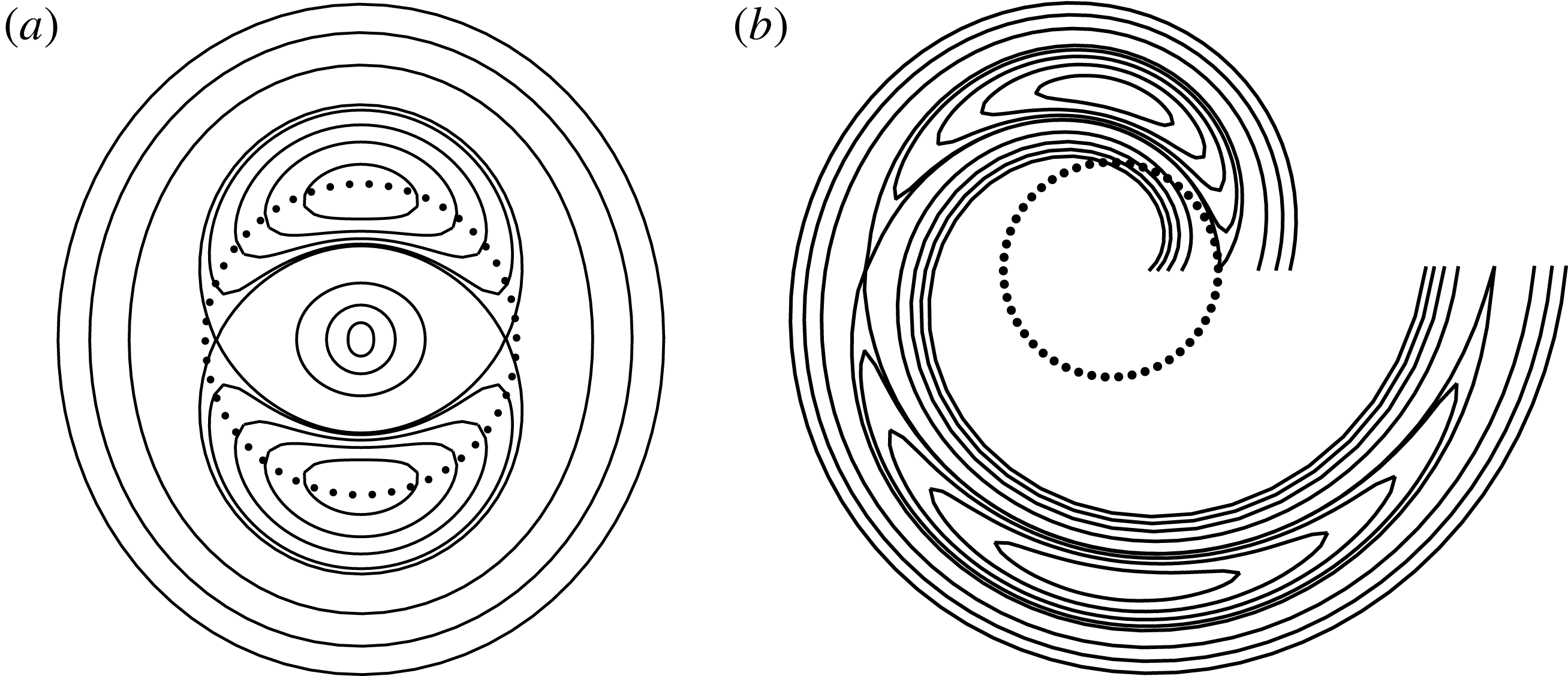
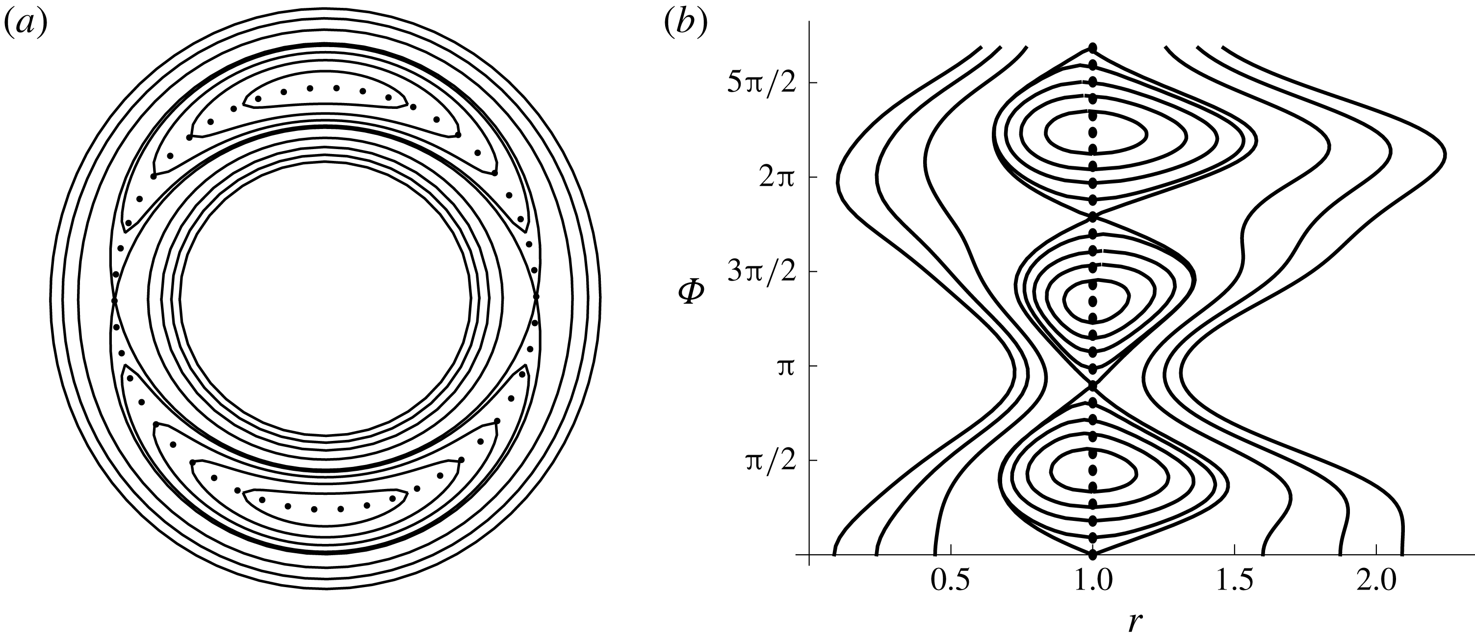
range (cf. figures 1–3). At each vortex height, a ‘cat’s eye’ pattern thus appears within these cylindrical cavities, exhibiting a recirculating flow.
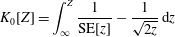
Sketch of a few streamline envelopes projected on a horizontal plane, spiralling around the critical radius
 $r_{c}$
(dotted line) on either side of the CL axis
 $r=r_{a}(\unicode[STIX]{x1D709},\unicode[STIX]{x1D6F7},\unicode[STIX]{x1D6E9})$
(dot–dashed line),
 $m=6$
.

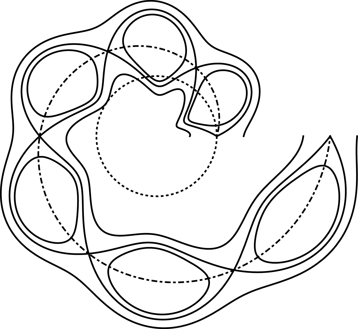
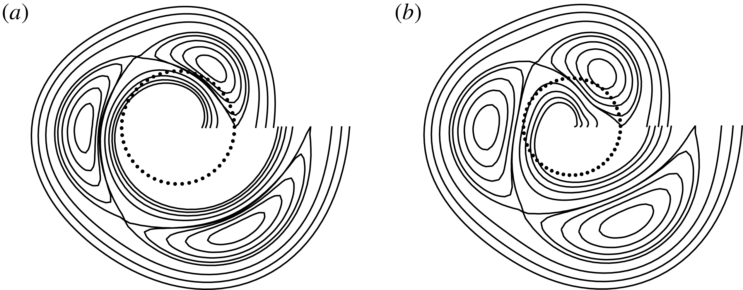
The vortex plus the wave packet
 $m=2$
and the various regions (bounded by dashed lines) in a horizontal plane: the core outer flow COF characterized by
 $\unicode[STIX]{x1D702}<0$
, the core inner flow CIF defined by
 $s=-$
and
 $Z>A$
, the cat’s eye flow CEF defined by
 $Z\leqslant A$
, the external inner flow EIF defined by
 $s=+$
and
 $Z>A$
, and the external outer flow EOF defined by
 $\unicode[STIX]{x1D702}>0$
. The CL involves CIF
 $+$
CEF
 $+$
EIF. The dotted line represents the critical radius
 $r_{c}$
and the dot–dashed line is the CL symmetry radius
 $r_{a}$
.

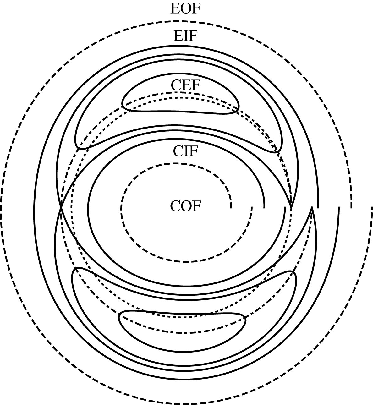
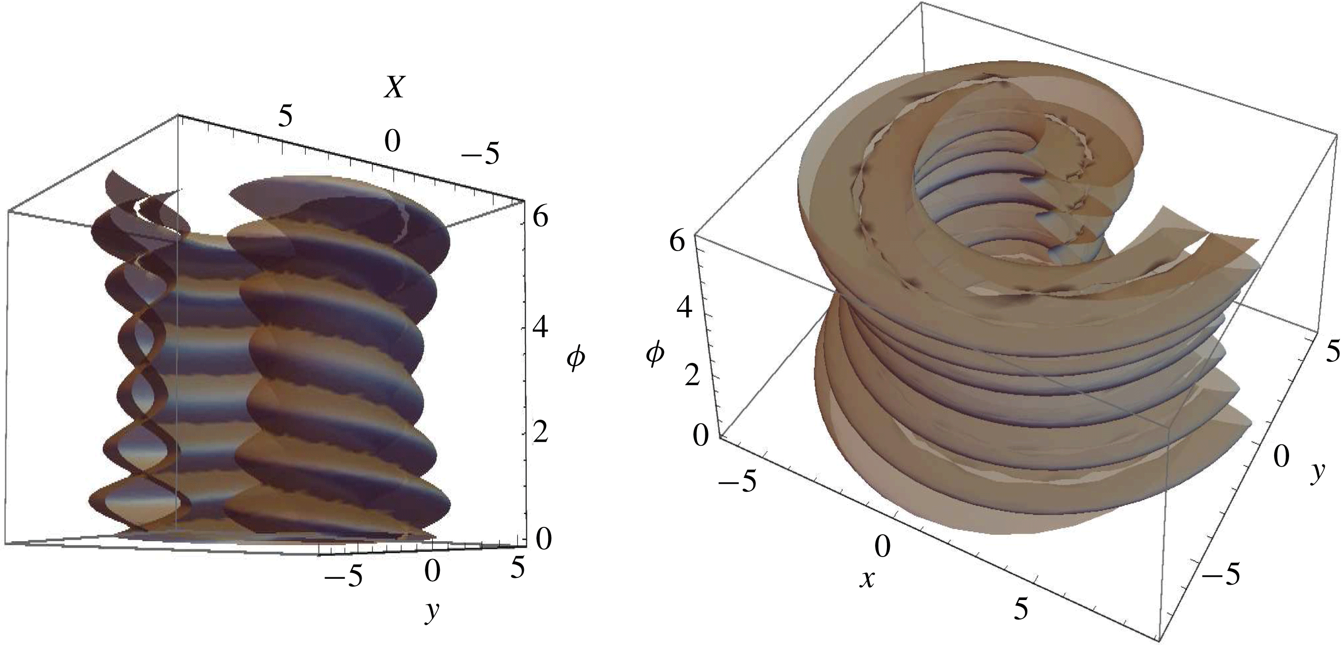
Separatrices
 $Z=A$
as functions of
 $x,y$
and
 $\unicode[STIX]{x1D6F7}$
,
 $m=2$
,
 $\unicode[STIX]{x1D716}=0.1$
,
 $\unicode[STIX]{x1D71B}=2$
,
 $r_{c}=2$
,
 ${\mathcal{U}}_{2}=1$
,
 ${\mho}_{0}=0.5$
,
 $A(\unicode[STIX]{x1D6F7})=[1+\cos (\unicode[STIX]{x1D6F7})/2]^{2}$
.

The extended three-dimensional Prandtl–Batchelor theorem predicts in the steady-state assumption a leading-order uniform axial vorticity inside the separatrices (Caillol Reference Caillol2014); this result is no longer valid here. A Galerkin method is required to integrate the motion equations within the cat’s eye. A unique inviscid CL solution is found at the non-trivial expansion order by first applying secularity conditions on both inviscid and viscous inner flows, then matching both outer and inner flows on the CL edges, and finally matching the inner flow on the separatrices (cf. figure 2). The second part of the study will be presented in a separate paper. We will derive the system of leading-order nonlinear PDEs that governs the slowly evolving amplitudes of the wave packet and CL-induced mean flow. The numerical resolution of the system will reveal a lot of information about the evolution of the wave packet and vortex in the quasi-steady stage.
The paper is hence organized as follows. Section 2 describes the general outer-flow perturbation and phase-averaged equations. Section 3 gives the low-order, outer-flow asymptotic solutions through Frobenius series. Section 4 formulates the CL motion and gives the two first inner-flow orders. Section 5 examines the low-order CL-induced mean flow. Section 6 describes the first non-trivial inner-flow order strongly altered by the presence of the leading-order mean radial velocity. Section 7 presents numerical results of § 6. Section 8 gives the conclusion.
2 Formulation and main assumptions
We consider the motion of an unbounded, axisymmetric, columnar and linearly stable vortex on the
 $f$
-plane in a slightly viscous, incompressible and dry atmosphere. We use the cylindrical coordinates (
 $r,\unicode[STIX]{x1D703},z$
), with the variable
 $z$
being related to the height of the vortex along its rotation axis and
 $(u,v,w)$
being the velocity vector in these coordinates. Quantities have been made dimensionless through characteristic velocity and length scales: the maximum rotational wind of the vortex
 $V_{mw}$
and the maximum wind radius
 $R_{mw}$
. The related Reynolds number is
 $Re=V_{mw}R_{mw}/\unicode[STIX]{x1D708}$
, where
 $\unicode[STIX]{x1D708}$
is the kinematic viscosity. The inertial force
 $\boldsymbol{f}_{i}$
due to the rotating framework is
 $\boldsymbol{f}_{i}=v/r\,(v\,\boldsymbol{e}_{r}-u\,\boldsymbol{e}_{\unicode[STIX]{x1D703}})$
. The geopotential (the Earth-rotation-driven centrifugal force and gravity) with pressure
 $p$
is inserted into the gradient force to form the variable
 $\unicode[STIX]{x1D6E4}$
, defined by
 $\unicode[STIX]{x1D6E4}=p+gz-Co^{2}/8r^{2}$
and erroneously called geopotential. A constant value of the Coriolis parameter
 $Co=(fR_{mw})/V_{mw}$
is used throughout the study. The dimensionless equations governing this motion are the momentum and mass conservation equations in the ground-based frame of reference:
 $$\begin{eqnarray}\displaystyle \left.\begin{array}{@{}c@{}}\displaystyle \unicode[STIX]{x2202}_{t}\boldsymbol{u}+\boldsymbol{u}\boldsymbol{\cdot }\unicode[STIX]{x1D735}\boldsymbol{u}+Co\,\boldsymbol{z}\times \boldsymbol{u}=\boldsymbol{f}_{i}-\unicode[STIX]{x1D735}\unicode[STIX]{x1D6E4}+\frac{1}{Re}\unicode[STIX]{x0394}\boldsymbol{u}+\boldsymbol{F},\\ \displaystyle \text{D}^{\ast }u+\frac{1}{r}\unicode[STIX]{x2202}_{\unicode[STIX]{x1D703}}v+\unicode[STIX]{x2202}_{z}w=0,\quad \text{D}^{\ast }\bullet =\unicode[STIX]{x2202}_{r}\bullet +\frac{1}{r}\bullet .\end{array}\right\} & & \displaystyle\end{eqnarray}$$
The velocities and geopotential are decomposed between the wave-phase-averaged flow and the asymmetric perturbations in the following form:
 $$\begin{eqnarray}\displaystyle \left.\begin{array}{@{}c@{}}\displaystyle u=\overline{U}(r,\unicode[STIX]{x1D6E9},\unicode[STIX]{x1D6F7})+\unicode[STIX]{x1D716}\,U_{r}(\unicode[STIX]{x1D709},r,\unicode[STIX]{x1D6E9},\unicode[STIX]{x1D6F7}),\quad v=\overline{V}(r,\unicode[STIX]{x1D6E9},\unicode[STIX]{x1D6F7})+\unicode[STIX]{x1D716}\,U_{\unicode[STIX]{x1D703}}(\unicode[STIX]{x1D709},r,\unicode[STIX]{x1D6E9},\unicode[STIX]{x1D6F7}),\\ \displaystyle w=\overline{W}(r,\unicode[STIX]{x1D6E9},\unicode[STIX]{x1D6F7})+\unicode[STIX]{x1D716}\,U_{z}(\unicode[STIX]{x1D709},r,\unicode[STIX]{x1D6E9},\unicode[STIX]{x1D6F7}),\quad \unicode[STIX]{x1D6E4}=\overline{\unicode[STIX]{x1D6E4}}(r,\unicode[STIX]{x1D6E9},\unicode[STIX]{x1D6F7})+\unicode[STIX]{x1D716}\,P(\unicode[STIX]{x1D709},r,\unicode[STIX]{x1D6E9},\unicode[STIX]{x1D6F7}),\end{array}\right\} & & \displaystyle\end{eqnarray}$$
where the wave phase is
 $\unicode[STIX]{x1D709}=kz+m\unicode[STIX]{x1D703}-\unicode[STIX]{x1D714}t$
, with
 $k$
and
 $m$
respectively the axial and azimuthal wavenumbers. The overbar notation defines the phase-averaged quantity
 $q$
,
 $\overline{q}=1/(2\unicode[STIX]{x03C0})\int _{0}^{2\unicode[STIX]{x03C0}}q\,\text{d}\unicode[STIX]{x1D709}$
. The secular variable
 $\unicode[STIX]{x1D6E9}=m\unicode[STIX]{x1D703}$
characterizes the spiral motion. The leading-order perturbation is namely an amplitude-modulated, free vortical mode whose small dimensionless amplitude is
 $\unicode[STIX]{x1D716}$
and whose real and slowly evolving frequency is
 $\unicode[STIX]{x1D714}$
. The dimensionless wave phase tilt is denoted by
 $\unicode[STIX]{x1D71B}=kr_{c}/m$
and is taken as
 $O(1)$
or smaller. The mode is neutral and singular in the nonlinear theory, while it is assumed stable in the linear theory provided certain conditions are satisfied in the basic-state vorticity profile (Caillol Reference Caillol2015). We consider that wave packets propagate episodically in the vortex when they are excited by convective pulses. The mode is then supposed to be generated by an initial, localized and short-time forcing: for example, an impulse or a step-like condition. We assume a quasi-steady asymptotic state, so the fast time
 $t$
only appears in the phase
 $\unicode[STIX]{x1D709}$
, with the WMFI evolving at the slow time scales
 $T_{i}=\unicode[STIX]{x1D716}^{i/2}t$
,
 $i=1,2$
, that are omitted in the notations. The quasi-steady-state assumption is not restrictive since it is often observed among large-scale vortices due to a balance between friction in the boundary layer and sea–air exchanges (Emanuel Reference Emanuel1985). However, for the sake of simplicity, these effects will not be modelled in the following equations. We will study the WMFI above the surface boundary layer in order to neglect the effects of the latter on the interaction and to neglect the mean radial flow of the inflow layer (Zhang et al.
Reference Zhang, Rogers, Nolan and Marks2011). We will simply introduce the body force
 $\boldsymbol{F}$
, which permits one to exclude viscous diffusion effects on the basic-state vortex evolution without altering the inner flow, to the benefit of the WMFI.
The critical layer imposes its own scalings. The wave packet must be advected by the leading-order
 $O(\unicode[STIX]{x1D716}^{1/2})$
CL-induced mean vertical velocity, which leads to a time scale
 $T_{2}$
faster than the usual time
 $T_{3}$
for the Korteweg–de-Vries equation (Leibovich Reference Leibovich1970). The amplitude modulation space and time variables are hence
 $$\begin{eqnarray}\displaystyle \unicode[STIX]{x1D6F7}=\unicode[STIX]{x1D716}^{1/2}\frac{m}{r_{c}}\,z\quad \text{and}\quad \unicode[STIX]{x1D70F}_{2}\equiv T_{2}. & & \displaystyle\end{eqnarray}$$
Note that for the larger wave envelope in C17, the scalings were slower
 $(\unicode[STIX]{x1D6F7}\equiv \unicode[STIX]{x1D716}z,\unicode[STIX]{x1D70F}_{3}\equiv T_{3})$
. In this multiple-scale approach, the various partial derivatives are computed in the following way:
 $$\begin{eqnarray}\displaystyle \unicode[STIX]{x2202}_{\unicode[STIX]{x1D703}}\bullet =m(\unicode[STIX]{x2202}_{\unicode[STIX]{x1D709}}\bullet +\unicode[STIX]{x2202}_{\unicode[STIX]{x1D6E9}}\bullet ),\quad \unicode[STIX]{x2202}_{z}\bullet =\unicode[STIX]{x1D716}^{1/2}\frac{m}{r_{c}}\unicode[STIX]{x2202}_{\unicode[STIX]{x1D6F7}}\bullet +\tilde{k}\,\unicode[STIX]{x2202}_{\unicode[STIX]{x1D709}}\bullet ,\quad \unicode[STIX]{x2202}_{t}\bullet =\unicode[STIX]{x1D716}^{1/2}\unicode[STIX]{x2202}_{T_{1}}\bullet +\unicode[STIX]{x1D716}\,\unicode[STIX]{x2202}_{T_{2}}\bullet -\tilde{\unicode[STIX]{x1D714}}\,\unicode[STIX]{x2202}_{\unicode[STIX]{x1D709}}\bullet . & & \displaystyle \nonumber\\ \displaystyle & & \displaystyle\end{eqnarray}$$
The modulation-modified wavenumber and frequency are
 $\tilde{k}=k-m/r_{c}\,\unicode[STIX]{x1D714}_{\unicode[STIX]{x1D6F7}}\,T_{1}$
and
 $\tilde{\unicode[STIX]{x1D714}}=\unicode[STIX]{x1D714}+\unicode[STIX]{x1D716}^{1/2}\unicode[STIX]{x1D714}_{T_{2}}\,T_{1}$
. In spite of the smaller vertical scale of the wave envelope with respect to C17, the chosen regime is still the nonlinear critical layer, and wave packet linear effects like dispersion do not prevail (Mallier & Maslowe Reference Mallier and Maslowe1999; Campbell Reference Campbell2004).
The system of equations (2.1) after the decomposition (2.2) yields two subsystems of equations: the first describing the evolution of the perturbations, equations (2.5a–d ), and the second the evolution of the mean flow, equations (2.6a–d ).
 $$\begin{eqnarray}\displaystyle \frac{\text{D}U_{r}}{\text{D}t} & = & \displaystyle \unicode[STIX]{x1D71A}U_{\unicode[STIX]{x1D703}}-\text{D}[P+\overline{U}U_{r}]-\left(\frac{U_{\unicode[STIX]{x1D703}}}{r}\unicode[STIX]{x2202}_{\unicode[STIX]{x1D703}}+U_{z}\,\unicode[STIX]{x2202}_{z}\right)\overline{U}+\frac{\unicode[STIX]{x1D716}}{r}(U_{\unicode[STIX]{x1D703}}^{2}-\overline{U_{\unicode[STIX]{x1D703}}^{2}})\nonumber\\ \displaystyle & & \displaystyle +\,\unicode[STIX]{x1D716}\text{D}^{\ast }[\overline{U_{r}^{2}}]+\unicode[STIX]{x1D716}\,\unicode[STIX]{x2202}_{z}\overline{U_{z}U_{r}}+\frac{1}{Re}\left[\unicode[STIX]{x0394}U_{r}-\frac{U_{r}}{r^{2}}-\frac{2}{r^{2}}\unicode[STIX]{x2202}_{\unicode[STIX]{x1D703}}U_{\unicode[STIX]{x1D703}}\right],\end{eqnarray}$$
 $$\begin{eqnarray}\displaystyle \frac{\text{D}U_{\unicode[STIX]{x1D703}}}{\text{D}t} & = & \displaystyle -Q_{z}U_{r}-\overline{U}\text{D}^{\ast }[U_{\unicode[STIX]{x1D703}}]-\frac{\unicode[STIX]{x2202}_{\unicode[STIX]{x1D703}}P}{r}-\left(\frac{U_{\unicode[STIX]{x1D703}}}{r}\unicode[STIX]{x2202}_{\unicode[STIX]{x1D703}}+U_{z}\,\unicode[STIX]{x2202}_{z}\right)\overline{V}+\frac{\unicode[STIX]{x1D716}}{r^{2}}\text{D}[r^{2}\overline{U_{r}U_{\unicode[STIX]{x1D703}}}]\nonumber\\ \displaystyle & & \displaystyle -\,\unicode[STIX]{x1D716}\,\frac{U_{\unicode[STIX]{x1D703}}}{r}U_{r}+\unicode[STIX]{x1D716}\,\unicode[STIX]{x2202}_{z}\overline{U_{z}U_{\unicode[STIX]{x1D703}}}+\frac{1}{Re}\left[\unicode[STIX]{x0394}U_{\unicode[STIX]{x1D703}}-\frac{U_{\unicode[STIX]{x1D703}}}{r^{2}}+\frac{2}{r^{2}}\unicode[STIX]{x2202}_{\unicode[STIX]{x1D703}}U_{r}\right],\end{eqnarray}$$
 $$\begin{eqnarray}\displaystyle \frac{\text{D}U_{z}}{\text{D}t} & = & \displaystyle Q_{\unicode[STIX]{x1D703}}U_{r}-\overline{U}\text{D}[U_{z}]-\unicode[STIX]{x2202}_{z}P-\left(\frac{U_{\unicode[STIX]{x1D703}}}{r}\unicode[STIX]{x2202}_{\unicode[STIX]{x1D703}}+U_{z}\,\unicode[STIX]{x2202}_{z}\right)\overline{W}+\unicode[STIX]{x1D716}\text{D}^{\ast }[\overline{U_{r}U_{z}}]\nonumber\\ \displaystyle & & \displaystyle +\,\unicode[STIX]{x1D716}\,\unicode[STIX]{x2202}_{z}\overline{U_{z}^{2}}+\frac{1}{Re}\unicode[STIX]{x0394}U_{z},\end{eqnarray}$$
 $$\begin{eqnarray}\displaystyle \text{D}^{\ast }U_{r}+\frac{1}{r}\unicode[STIX]{x2202}_{\unicode[STIX]{x1D703}}U_{\unicode[STIX]{x1D703}}+\unicode[STIX]{x2202}_{z}U_{z}=0. & & \displaystyle\end{eqnarray}$$
 $$\begin{eqnarray}\displaystyle & \displaystyle \frac{{\mathcal{D}}\overline{U}}{{\mathcal{D}}t}=\overline{V}(Co+\unicode[STIX]{x1D6FA})-\text{D}\left[\overline{\unicode[STIX]{x1D6E4}}+\frac{1}{2}\overline{U}^{2}\right]+\unicode[STIX]{x1D716}^{2}\left(\frac{\overline{U_{\unicode[STIX]{x1D703}}^{2}}}{r}-\text{D}^{\ast }[\overline{U_{r}^{2}}]\right)-\unicode[STIX]{x1D716}^{5/2}\frac{m}{r_{c}}\unicode[STIX]{x2202}_{\unicode[STIX]{x1D6F7}}\overline{U_{z}U_{r}}+\frac{\unicode[STIX]{x1D6E5}_{r}}{Re}\overline{U}, & \displaystyle \nonumber\\ \displaystyle & & \displaystyle\end{eqnarray}$$
 $$\begin{eqnarray}\displaystyle & \displaystyle \frac{{\mathcal{D}}\overline{V}}{{\mathcal{D}}t}=-Q_{z}\overline{U}-\frac{m}{r}\unicode[STIX]{x2202}_{\unicode[STIX]{x1D6E9}}\overline{\unicode[STIX]{x1D6E4}}-\frac{\unicode[STIX]{x1D716}^{2}}{r^{2}}\text{D}[r^{2}\overline{U_{r}U_{\unicode[STIX]{x1D703}}}]-\unicode[STIX]{x1D716}^{5/2}\frac{m}{r_{c}}\unicode[STIX]{x2202}_{\unicode[STIX]{x1D6F7}}\overline{U_{z}U_{\unicode[STIX]{x1D703}}}+\frac{\unicode[STIX]{x1D6E5}_{r}}{Re}\overline{V}+F_{\unicode[STIX]{x1D703}}, & \displaystyle\end{eqnarray}$$
 $$\begin{eqnarray}\displaystyle & \displaystyle \frac{{\mathcal{D}}\overline{W}}{{\mathcal{D}}t}=Q_{\unicode[STIX]{x1D703}}\overline{U}-\unicode[STIX]{x1D716}^{1/2}\frac{m}{r_{c}}\unicode[STIX]{x2202}_{\unicode[STIX]{x1D6F7}}[\overline{\unicode[STIX]{x1D6E4}}+\unicode[STIX]{x1D716}^{2}\overline{U_{z}^{2}}]-\unicode[STIX]{x1D716}^{2}\text{D}^{\ast }[\overline{U_{r}U_{z}}]+\frac{1}{Re}\left(\unicode[STIX]{x1D6E5}_{r}\overline{W}+\frac{\overline{W}}{r^{2}}\right), & \displaystyle\end{eqnarray}$$
 $$\begin{eqnarray}\displaystyle & \displaystyle \text{D}^{\ast }\overline{U}+m\frac{\unicode[STIX]{x2202}_{\unicode[STIX]{x1D6E9}}\overline{V}}{r}+\unicode[STIX]{x1D716}^{1/2}\frac{m}{r_{c}}\unicode[STIX]{x2202}_{\unicode[STIX]{x1D6F7}}\overline{W}=0. & \displaystyle\end{eqnarray}$$
 $\unicode[STIX]{x2202}_{\unicode[STIX]{x1D6E9}}\overline{U_{\unicode[STIX]{x1D703}}U_{r}},\unicode[STIX]{x2202}_{\unicode[STIX]{x1D6E9}}\overline{U_{\unicode[STIX]{x1D703}}^{2}},\ldots$
have been omitted in (2.5) and (2.6) because they appear at high orders and are negligible in this study. The system (2.5) is coupled with the following boundary conditions:
 $$\begin{eqnarray}\displaystyle \left.\begin{array}{@{}c@{}}\displaystyle r\rightarrow \infty ,\quad (U_{r},\,U_{\unicode[STIX]{x1D703}},\,U_{z},\,P)\rightarrow (0,0,0,0);\\ \displaystyle r\rightarrow 0,\quad U_{\unicode[STIX]{x1D703}}\rightarrow 0,\quad \text{and}\quad \text{if}~|m|\neq 1,\quad U_{r}\rightarrow 0.\end{array}\right\} & & \displaystyle\end{eqnarray}$$
The CL-induced mean flow expands in two spiralling helical diffusion boundary layers on either side of the CL, and vanishes far from
 $r_{c}$
. No boundary condition is specified in the vertical direction. The circular vortex is characterized by the mean angular rotation
 $\unicode[STIX]{x1D6FA}(r)=\overline{V}(r)/r$
, the absolute mean axial vorticity
 $Q_{z}(r)=1/r\text{D}[r\overline{V}(r)]+Co$
, the mean azimuthal vorticity
 $Q_{\unicode[STIX]{x1D703}}(r)=-\overline{W}^{\prime }(r)$
and the absolute inertial frequency
 $\unicode[STIX]{x1D71A}(r)=2\unicode[STIX]{x1D6FA}(r)+Co$
. The prime denotes the radial derivative of the phase-averaged quantities when it is not specified, otherwise D denotes the radial differential operator. We also have the different notations
 $$\begin{eqnarray}\displaystyle \left.\begin{array}{@{}c@{}}\displaystyle \frac{\text{D}}{\text{D}t}\bullet =\unicode[STIX]{x2202}_{t}\bullet +\unicode[STIX]{x1D716}\,\left[U_{r}\unicode[STIX]{x2202}_{r}+\frac{U_{\unicode[STIX]{x1D703}}}{r}\,\unicode[STIX]{x2202}_{\unicode[STIX]{x1D703}}+U_{z}\,\unicode[STIX]{x2202}_{z}\right]\bullet +\unicode[STIX]{x1D6FA}\,\unicode[STIX]{x2202}_{\unicode[STIX]{x1D703}}\bullet +\overline{W}\unicode[STIX]{x2202}_{z}\bullet ,\\ \displaystyle \unicode[STIX]{x0394}_{r}\bullet =\text{D}[\text{D}^{\ast }[\bullet ]]+\unicode[STIX]{x1D716}\frac{m^{2}}{r_{c}^{2}}\unicode[STIX]{x2202}_{\unicode[STIX]{x1D6F7}}^{2}\bullet ,\\ \displaystyle \frac{{\mathcal{D}}}{{\mathcal{D}}t}\bullet =\unicode[STIX]{x1D716}\,\unicode[STIX]{x2202}_{T_{2}}\bullet +m\unicode[STIX]{x1D6FA}\,\unicode[STIX]{x2202}_{\unicode[STIX]{x1D6E9}}\bullet +\unicode[STIX]{x1D716}^{1/2}\frac{m}{r_{c}}\overline{W}\unicode[STIX]{x2202}_{\unicode[STIX]{x1D6F7}}\bullet ,\\ \displaystyle \unicode[STIX]{x0394}\bullet =\text{D}^{\ast }[\text{D}[\bullet ]]+\frac{1}{r^{2}}\unicode[STIX]{x2202}_{\unicode[STIX]{x1D703}}^{2}\bullet +\unicode[STIX]{x2202}_{z}^{2}\bullet ,\quad \text{and}\quad \frac{1}{Re}=\unicode[STIX]{x1D706}\,\unicode[STIX]{x1D716}^{3/2}.\end{array}\right\} & & \displaystyle\end{eqnarray}$$
Here, we use the nonlinear CL theory, so we will assume that the Haberman parameter
 $\unicode[STIX]{x1D706}$
, the cubic ratio of the viscous CL thickness to the nonlinear CL thickness, is small:
 $\unicode[STIX]{x1D706}\ll 1$
when it is not indicated, which allows for a
 $\unicode[STIX]{x1D706}$
-expansion of the flow, dividing it into an inviscid part and a smaller viscous part, for instance, for the radial velocity
 $U=U_{r,i}+\unicode[STIX]{x1D706}U_{r,v}+o(\unicode[STIX]{x1D706})$
. The perturbations of velocity, geopotential and vorticity are expanded in terms of the square root of the wave packet amplitude, for instance, for the radial velocity
 $$\begin{eqnarray}\displaystyle U_{r}=U_{r}^{(0)}+\unicode[STIX]{x1D716}^{1/2}\,U_{r}^{(1)}+\unicode[STIX]{x1D716}\,U_{r}^{(2)}+\cdots \,, & & \displaystyle\end{eqnarray}$$
with the zeroth order characterizing the amplitude-modulated non-normal vorticity mode. Although large vertical and radial velocities may occur in tropical cyclones above the inflow layer, these are always smaller than the rotational velocities (Reasor et al.
Reference Reasor, Montgomery, Marks and Gamache2000) and we will thus assume that the basic-state vortex only contains a field of mean azimuthal velocity. The WMF interaction will nevertheless induce mean vertical and radial velocity fields. As a result, the mean radial, azimuthal and axial shear flows are expanded in terms of
 $\unicode[STIX]{x1D716}^{1/2}$
in the same way, such as the frequency
 $\unicode[STIX]{x1D714}(\unicode[STIX]{x1D6F7})=\unicode[STIX]{x1D714}_{0}+\unicode[STIX]{x1D716}^{1/2}\unicode[STIX]{x1D714}_{1}(\unicode[STIX]{x1D6F7})+\unicode[STIX]{x1D716}\,\unicode[STIX]{x1D714}_{2}(\unicode[STIX]{x1D6F7})+\cdots \,$
 $$\begin{eqnarray}\displaystyle & \displaystyle \overline{U}=\unicode[STIX]{x1D716}\,\overline{U}_{2}(r,\unicode[STIX]{x1D6E9},\unicode[STIX]{x1D6F7})+\unicode[STIX]{x1D716}^{3/2}\,\overline{U}_{3}(r,\unicode[STIX]{x1D6E9},\unicode[STIX]{x1D6F7})+\cdots \,, & \displaystyle\end{eqnarray}$$
 $$\begin{eqnarray}\displaystyle & \displaystyle \overline{V}=\overline{V}_{0}(r)+\unicode[STIX]{x1D716}^{1/2}\overline{V}_{1}(r,\unicode[STIX]{x1D6E9},\unicode[STIX]{x1D6F7})+\unicode[STIX]{x1D716}\,\overline{V}_{2}(r,\unicode[STIX]{x1D6E9},\unicode[STIX]{x1D6F7})+\unicode[STIX]{x1D716}^{3/2}\,\overline{V}_{3}(r,\unicode[STIX]{x1D6E9},\unicode[STIX]{x1D6F7})+\cdots \,, & \displaystyle\end{eqnarray}$$
 $$\begin{eqnarray}\displaystyle & \displaystyle \overline{W}=\unicode[STIX]{x1D716}^{1/2}\overline{W}_{1}(r,\unicode[STIX]{x1D6E9},\unicode[STIX]{x1D6F7})+\unicode[STIX]{x1D716}\,\overline{W}_{2}(r,\unicode[STIX]{x1D6E9},\unicode[STIX]{x1D6F7})+\unicode[STIX]{x1D716}^{3/2}\,\overline{W}_{3}(r,\unicode[STIX]{x1D6E9},\unicode[STIX]{x1D6F7})+\cdots \,, & \displaystyle\end{eqnarray}$$
 $$\begin{eqnarray}\displaystyle & \displaystyle Q_{z}=Q_{0}(r)+\unicode[STIX]{x1D716}^{1/2}Q_{z,1}(r,\unicode[STIX]{x1D6E9},\unicode[STIX]{x1D6F7})+\unicode[STIX]{x1D716}\,Q_{z,2}(r,\unicode[STIX]{x1D6E9},\unicode[STIX]{x1D6F7})+\cdots \,, & \displaystyle\end{eqnarray}$$
 $$\begin{eqnarray}\displaystyle & \displaystyle Q_{\unicode[STIX]{x1D703}}=\unicode[STIX]{x1D716}^{1/2}Q_{\unicode[STIX]{x1D703},1}(r,\unicode[STIX]{x1D6E9},\unicode[STIX]{x1D6F7})+\unicode[STIX]{x1D716}\,Q_{\unicode[STIX]{x1D703},2}(r,\unicode[STIX]{x1D6E9},\unicode[STIX]{x1D6F7})+\cdots \,. & \displaystyle\end{eqnarray}$$
 $O(1)$
phase-averaged rotational flow at the end of the transition stage, resulting from the strong interaction between the basic vortex and the wave packet. As
 $|r-r_{c}|\rightarrow \infty$
, the zeroth-order mean flow tends to the basic vortex. The body force is thus
 $F_{\unicode[STIX]{x1D703}}(r)=-Q_{0}^{\prime }(r)/Re$
. We also assume that the expansion of
 $Co$
is restricted to the first order:
 $Co=Co_{0}+\unicode[STIX]{x1D716}^{1/2}Co_{1}$
. The mean geopotential is determined by (2.6a
) and to the first orders are defined by the gradient wind balance
 $$\begin{eqnarray}\displaystyle & \displaystyle \overline{\unicode[STIX]{x1D6E4}}_{0}={\textstyle \frac{1}{8}}(\unicode[STIX]{x1D71A}_{0,c}^{2}-Co_{0}^{2})r_{c}^{2}+{\textstyle \frac{1}{4}}\int _{r_{c}}^{r}\unicode[STIX]{x1D71A}_{0}^{2}(r)-Co_{0}^{2}\,r\,\text{d}r, & \displaystyle\end{eqnarray}$$
 $$\begin{eqnarray}\displaystyle & \displaystyle \overline{\unicode[STIX]{x1D6E4}}_{1}=\overline{\unicode[STIX]{x1D6E4}}_{1}(r_{c})+{\textstyle \frac{1}{2}}\int _{r_{c}}^{r}\unicode[STIX]{x1D71A}_{0}\unicode[STIX]{x1D71A}_{1}-Co_{0}Co_{1}\,r\,\text{d}r, & \displaystyle\end{eqnarray}$$
 $$\begin{eqnarray}\displaystyle & \displaystyle \overline{\unicode[STIX]{x1D6E4}}_{2}=\overline{\unicode[STIX]{x1D6E4}}_{2}(r_{c})+{\textstyle \frac{1}{2}}\int _{r_{c}}^{r}\unicode[STIX]{x1D71A}_{0}\unicode[STIX]{x1D71A}_{2}+{\textstyle \frac{1}{2}}(\unicode[STIX]{x1D71A}_{1}^{2}-Co_{1}^{2})\,r\,\text{d}r. & \displaystyle\end{eqnarray}$$
3 The outer flow
In this section, we give the outer-flow asymptotic solution near
 $r_{c}$
, which will be useful to determine the CL flow in a unique way through matchings with the outer flow.
The spiralling motion shifts the CL symmetry axis from the critical radius; this difficulty is overcome here by introducing a coordinate
 $\unicode[STIX]{x1D702}$
which is constant along a streamline (Davis Reference Davis1969). As a result, the representation, in cylindrical coordinates, of a streamline is
 $$\begin{eqnarray}\displaystyle r=r_{c}+\unicode[STIX]{x1D702}+h(\unicode[STIX]{x1D702},\unicode[STIX]{x1D709},\unicode[STIX]{x1D6E9},\unicode[STIX]{x1D6F7}), & & \displaystyle\end{eqnarray}$$
where the deviation
 $h$
from axisymmetry is assumed to be of order
 $\unicode[STIX]{x1D716}$
(cf. figures 1 and 2). Owing to the decay of vorticity inside the CL occurring during the WMFI, we assume that the basic-vortex axial vorticity becomes zero on the CL axis
 $r_{a}=r(\unicode[STIX]{x1D702}=0)$
a long time after the beginning of the interaction, but before the quasi-steady stage starts:
 $$\begin{eqnarray}\displaystyle Q_{0}=0\quad \text{at}~r=r_{a}(\unicode[STIX]{x1D709},\unicode[STIX]{x1D6E9},\unicode[STIX]{x1D6F7})=r_{c}+h(0,\unicode[STIX]{x1D709},\unicode[STIX]{x1D6E9},\unicode[STIX]{x1D6F7}). & & \displaystyle\end{eqnarray}$$
3.1 The amplitude-modulated singular mode
The linearized, inviscid and stationary system (2.5) can be reduced to a single equation, the Howard–Gupta modal equation generalized to the
 $f$
-plane and related to the modal radial velocity
 $U_{r}^{(0)}$
(Howard & Gupta Reference Howard and Gupta1962). This is expressed as
 ${\mathcal{L}}_{0}(U_{r}^{(0)})=0$
, namely
 $$\begin{eqnarray}\displaystyle \text{D}[S(r)\text{D}^{\ast }U_{r}^{(0)}]+\unicode[STIX]{x2202}_{\unicode[STIX]{x1D709}}^{2}U_{r}^{(0)}+\left((r\text{D}-2)[S(r)Q_{0}(r)]+\frac{k^{2}r^{2}\unicode[STIX]{x1D71A}_{0}(r)}{m\unicode[STIX]{x1D714}_{0}^{D}(r)}S(r)Q_{0}(r)\right)\frac{m\,U_{r}^{(0)}}{\unicode[STIX]{x1D714}_{0}^{D}(r)r^{2}}=0. & & \displaystyle \nonumber\\ \displaystyle & & \displaystyle\end{eqnarray}$$
The superscript
 $D$
defines the Doppler-shifted frequency
 $$\begin{eqnarray}\displaystyle \unicode[STIX]{x1D714}^{D}(r)=\tilde{\unicode[STIX]{x1D714}}-m\unicode[STIX]{x1D6FA}(r)-\tilde{k}\,\overline{W}(r),\quad S(r)=\frac{r^{2}}{m^{2}+k^{2}r^{2}}. & & \displaystyle\end{eqnarray}$$
Equation (3.3) is singular at the critical radius
 $r_{c}$
where the Doppler-shifted frequency
 $\unicode[STIX]{x1D714}_{0}^{D}(r)$
vanishes (that is,
 $\unicode[STIX]{x1D714}_{0}=m\unicode[STIX]{x1D6FA}_{0,c}$
). But the solution is weakly singular around
 $r_{c}$
, at the end of the strong vortex/wave packet interaction, since the local equivalent Richardson number
 $J(r)=(kr/m)^{2}\,\unicode[STIX]{x1D71A}_{0}(r)Q_{0}(r)/[Q_{0}(r)-\unicode[STIX]{x1D71A}_{0}(r)]^{2}$
becomes small near the CL symmetry axis
 $r_{a}$
, as the zeroth-order mean axial vorticity vanishes at
 $r_{a}$
. The connection of this number with the linear stability of a rotating sheared flow is evoked in Caillol (Reference Caillol2014, Reference Caillol2015). The subscript
 $c$
characterizes the critical radius.
The neutral-mode radial velocity evaluated on the streamline
 $\unicode[STIX]{x1D702}$
is expressed by two Frobenius series of the variable
 $r-r_{c}=\unicode[STIX]{x1D702}+h(\unicode[STIX]{x1D702})$
:
 $$\begin{eqnarray}\displaystyle U_{r}^{(0)}=\left(\frac{a}{r_{c}}\unicode[STIX]{x1D719}_{a}[\unicode[STIX]{x1D702}+h(\unicode[STIX]{x1D702})]+\unicode[STIX]{x1D719}_{b}[\unicode[STIX]{x1D702}+h(\unicode[STIX]{x1D702})]\right)\,U_{0}(\unicode[STIX]{x1D6F7})\,\sin \unicode[STIX]{x1D709}+\frac{C}{r_{c}}\unicode[STIX]{x1D719}_{a}[\unicode[STIX]{x1D702}+h(\unicode[STIX]{x1D702})]U_{0}(\unicode[STIX]{x1D6F7})\,\cos \unicode[STIX]{x1D709}, & & \displaystyle \nonumber\\ \displaystyle & & \displaystyle\end{eqnarray}$$
where both Frobenius series
 $\unicode[STIX]{x1D719}_{a}$
and
 $\unicode[STIX]{x1D719}_{b}$
are expanded around
 $r_{c}$
in the following way:
 $$\begin{eqnarray}\displaystyle \unicode[STIX]{x1D719}_{a}(\unicode[STIX]{x1D702})=\unicode[STIX]{x1D702}+\mathop{\sum }_{n=2}^{\infty }a_{0,n}\unicode[STIX]{x1D702}^{n},\quad \unicode[STIX]{x1D719}_{b}(\unicode[STIX]{x1D702})=1+\mathop{\sum }_{n=2}^{\infty }b_{0,n}\unicode[STIX]{x1D702}^{n}+b_{0}\unicode[STIX]{x1D719}_{a}(\unicode[STIX]{x1D702})\ln \unicode[STIX]{x1D702}^{\ast }. & & \displaystyle\end{eqnarray}$$
The radius
 $\unicode[STIX]{x1D702}$
inside the logarithm is normalized by
 $\unicode[STIX]{x1D702}^{\ast }=\unicode[STIX]{x1D702}/\unicode[STIX]{x1D702}_{0}$
, where
 $\unicode[STIX]{x1D702}_{0}=r_{c}/\sqrt{2}$
. The complex logarithmic function in (3.6b
) induces an additional, in-phase quadrature term in (3.5) as
 $r<r_{c}$
, caused by the logarithmic phase shift
 $\unicode[STIX]{x1D719}$
defining
 $C$
as follows:
 $$\begin{eqnarray}\displaystyle r>r_{c},\quad C^{+}=0,\quad \text{and}\quad r<r_{c},\quad C^{-}=b_{0}r_{c}\unicode[STIX]{x1D719}(\unicode[STIX]{x1D706}). & & \displaystyle\end{eqnarray}$$
The superscript
 $s=-$
will be used to characterize the vortex core, where
 $r<r_{c}$
, and the superscript
 $s=+$
the outer core, where
 $r>r_{c}$
.
3.2 Order
 $\unicode[STIX]{x1D716}^{3/2}$
outer flow

The first-order inviscid disturbance is decomposed into five contributions. The radial velocity
 $U_{r,i}^{(1)}$
can be then written as
 $$\begin{eqnarray}\displaystyle U_{r,i}^{(1)}=U_{r,h}^{(1)}+U_{r,l}^{(1)}+U_{r,d}^{(1)}+U_{r,ad}^{(1)}+U_{r,\unicode[STIX]{x1D714}d}^{(1)}. & & \displaystyle\end{eqnarray}$$
The first term constitutes a CL feedback into the outer flow. It is required while matching the inner flow on the separatrices. The second term
 $U_{r,l}^{(1)}$
is generated by the advection of the mode by the first-order mean flow. The three next terms
 $U_{r,d}^{(1)}$
,
 $U_{r,ad}^{(1)}$
and
 $U_{r,\unicode[STIX]{x1D714}d}^{(1)}$
are respectively created by the vertical gradients of the modal amplitude
 $U_{0}$
, the phase jump
 $a$
and the frequency
 $\unicode[STIX]{x1D714}_{1}$
. The velocities
 $U_{r,h}^{(1)}$
and
 $U_{r,\unicode[STIX]{x1D714}d}^{(1)}$
are not
 $\unicode[STIX]{x1D6E9}$
-secular at the lowest expansion order near
 $\unicode[STIX]{x1D702}=0$
. So their secularity can be neglected in the study. Differentiation with respect to
 $\unicode[STIX]{x1D6E9}$
in the system (2.5) leads to the presence of coupled sine and cosine eigenfunctions. The dependence of
 $U_{r,i}^{(1)}$
on the phase
 $\unicode[STIX]{x1D709}$
is hence as follows:
 $$\begin{eqnarray}\displaystyle U_{r,i}^{(1)}(r,\unicode[STIX]{x1D709}) & = & \displaystyle \{[\unicode[STIX]{x1D719}_{l}^{(1,1)}(r)+\unicode[STIX]{x1D714}_{1,\unicode[STIX]{x1D6F7}}T_{1}\,\unicode[STIX]{x1D719}_{\unicode[STIX]{x1D714}d}^{(1,1)}(r)+a_{\unicode[STIX]{x1D6F7}}\unicode[STIX]{x1D719}_{ad}^{(1,1)}(r)]\,U_{0}+\unicode[STIX]{x1D719}_{d}^{(1,1)}U_{0,\unicode[STIX]{x1D6F7}}\}\sin \unicode[STIX]{x1D709}\nonumber\\ \displaystyle & & \displaystyle +\,\{[\unicode[STIX]{x1D719}_{l}^{(1,2)}(r)+a_{\unicode[STIX]{x1D6F7}}\unicode[STIX]{x1D719}_{ad}^{(1,2)}(r)]\,U_{0}+\unicode[STIX]{x1D719}_{d}^{(1,2)}(r)\,U_{0,\unicode[STIX]{x1D6F7}}\}\cos \unicode[STIX]{x1D709}+\unicode[STIX]{x1D719}_{h}^{(1)}(r)\,U_{0}\cos (2\unicode[STIX]{x1D709}).\nonumber\\ \displaystyle & & \displaystyle\end{eqnarray}$$
The feedback flow satisfies the homogeneous equation
 $$\begin{eqnarray}\displaystyle {\mathcal{L}}_{0}(U_{r,h}^{(1)})=0,\quad \text{with}~\unicode[STIX]{x1D719}_{h}^{(1)}(\unicode[STIX]{x1D702})=\frac{\unicode[STIX]{x1D6FE}_{h,1}}{r_{c}}\unicode[STIX]{x1D719}_{a}(\unicode[STIX]{x1D702})+\unicode[STIX]{x1D705}_{h,1}\unicode[STIX]{x1D719}_{b}(\unicode[STIX]{x1D702}). & & \displaystyle\end{eqnarray}$$
The other terms satisfy non-homogeneous linear equations. The second contribution
 $U_{r,l}^{(1)}$
satisfies the equation
 $$\begin{eqnarray}\displaystyle \left.\begin{array}{@{}c@{}}{\mathcal{L}}_{0}(U_{r,l}^{(1,1)})=-{\mathcal{L}}_{1,1}(U_{r}^{(0)})-{\mathcal{L}}_{1,\unicode[STIX]{x1D703}}(\boldsymbol{U}_{l}^{(1,2)},P_{l}^{(1,2)}),\\ {\mathcal{L}}_{0}(U_{r,l}^{(1,2)})=-{\mathcal{L}}_{1,2}(U_{\unicode[STIX]{x1D703}}^{(0)})-{\mathcal{L}}_{1,\unicode[STIX]{x1D703}}(\boldsymbol{U}_{l}^{(1,1)},P_{l}^{(1,1)}),\end{array}\right\} & & \displaystyle\end{eqnarray}$$
with the operators
 ${\mathcal{L}}_{1,1}$
,
 ${\mathcal{L}}_{1,2}$
and
 ${\mathcal{L}}_{1,\unicode[STIX]{x1D703}}$
defined by
 $$\begin{eqnarray}\displaystyle {\mathcal{L}}_{1,1}(U) & = & \displaystyle \left\{(r\text{D}-2)\left[S(r)\left(Q_{z,1}(r)-\frac{kr}{m}Q_{\unicode[STIX]{x1D703},1}(r)\right)\right]\right.\nonumber\\ \displaystyle & & \displaystyle +\left.kr\frac{S(r)\unicode[STIX]{x1D71A}_{0}(r)}{\unicode[STIX]{x1D714}_{0}^{D}(r)}\left(\frac{kr}{m}Q_{z,1}(r)+Q_{\unicode[STIX]{x1D703},1}(r)\right)-\frac{\unicode[STIX]{x1D714}_{1}^{D}(r)}{\unicode[STIX]{x1D714}_{0}^{D}(r)}(r\text{D}-2)[S(r)Q_{0}(r)]\right.\nonumber\\ \displaystyle & & \displaystyle +\left.\frac{k^{2}r^{2}}{m}\frac{S(r)\unicode[STIX]{x1D71A}_{0}(r)}{\unicode[STIX]{x1D714}_{0}^{D}(r)}\left[\frac{\unicode[STIX]{x1D71A}_{1}(r)}{\unicode[STIX]{x1D71A}_{0}(r)}-2\frac{\unicode[STIX]{x1D714}_{1}^{D}(r)}{\unicode[STIX]{x1D714}_{0}^{D}(r)}\right]Q_{0}(r)\right\}\frac{mU}{\unicode[STIX]{x1D714}_{0}^{D}(r)r^{2}},\end{eqnarray}$$
and
 $$\begin{eqnarray}\displaystyle {\mathcal{L}}_{1,2}(U) & = & \displaystyle \frac{km\unicode[STIX]{x1D71A}_{0}(r)}{r\unicode[STIX]{x1D714}_{0}^{D2}(r)}S(r)U\unicode[STIX]{x2202}_{\unicode[STIX]{x1D6E9}}\left[k\overline{V}_{1}(r)-\frac{m}{r}\overline{W}_{1}(r)\right]\nonumber\\ \displaystyle & & \displaystyle +\,\frac{m}{\unicode[STIX]{x1D714}_{0}^{D}(r)}\text{D}\left[\frac{S(r)}{r}U\unicode[STIX]{x2202}_{\unicode[STIX]{x1D6E9}}\left[k\overline{W}_{1}(r)+\frac{m}{r}\overline{V}_{1}(r)\right]\right]\end{eqnarray}$$
 $$\begin{eqnarray}\displaystyle {\mathcal{L}}_{1,\unicode[STIX]{x1D703}}(U,P) & = & \displaystyle \frac{m\unicode[STIX]{x1D71A}_{0}(r)}{\unicode[STIX]{x1D714}_{0}^{D2}(r)}\left[\unicode[STIX]{x1D6FA}_{0}(r)-\unicode[STIX]{x1D714}_{0}\frac{m}{r^{2}}S(r)\right]\unicode[STIX]{x2202}_{\unicode[STIX]{x1D6E9}}U_{\unicode[STIX]{x1D703}}-m\frac{\unicode[STIX]{x1D6FA}_{0}(r)}{\unicode[STIX]{x1D714}_{0}^{D}(r)}\unicode[STIX]{x2202}_{\unicode[STIX]{x1D6E9}}\unicode[STIX]{x2202}_{\unicode[STIX]{x1D709}}U_{r}\nonumber\\ \displaystyle & & \displaystyle +\,k\frac{m}{r}\frac{\unicode[STIX]{x1D71A}_{0}(r)}{\unicode[STIX]{x1D714}_{0}^{D2}(r)}S(r)\unicode[STIX]{x2202}_{\unicode[STIX]{x1D6E9}}[kP-m\unicode[STIX]{x1D6FA}_{0}(r)U_{z}]\nonumber\\ \displaystyle & & \displaystyle +\,\frac{m\text{D}}{\unicode[STIX]{x1D714}_{0}^{D}(r)}\left[S(r)\unicode[STIX]{x2202}_{\unicode[STIX]{x1D6E9}}\left(\frac{m}{r^{2}}P+\frac{\unicode[STIX]{x1D714}_{0}}{r}U_{\unicode[STIX]{x1D703}}+k\unicode[STIX]{x1D6FA}_{0}(r)U_{z}\right)\right].\end{eqnarray}$$
The first-order Doppler-shifted frequency is
 $\unicode[STIX]{x1D714}_{1}^{D}(r)=\unicode[STIX]{x1D714}_{1}-m\unicode[STIX]{x1D6FA}_{1}(r)-k\overline{W}_{1}(r)$
. The first-order equivalent Richardson number, derived from (3.12), is given at
 $r=r_{c}$
by
 $$\begin{eqnarray}\displaystyle J_{1,c}=\frac{\unicode[STIX]{x1D71B}}{\unicode[STIX]{x1D71A}_{0,c}}(\unicode[STIX]{x1D71B}Q_{z,1,c}+Q_{\unicode[STIX]{x1D703},1,c})-(1+2\unicode[STIX]{x1D71B}^{2})\unicode[STIX]{x1D714}_{1,c}^{D}\frac{r_{c}Q_{z,0,c}^{\prime }}{m\unicode[STIX]{x1D71A}_{0,c}^{2}}. & & \displaystyle\end{eqnarray}$$
The radial velocities
 $U_{r,d}^{(1)}$
,
 $U_{r,ad}^{(1)}$
and
 $U_{r,\unicode[STIX]{x1D714}d}^{(1)}$
satisfy the equations
 $$\begin{eqnarray}\displaystyle & \displaystyle \left.\begin{array}{@{}c@{}}{\mathcal{L}}_{0}(U_{r,d}^{(1,1)})=-{\mathcal{L}}_{1,\unicode[STIX]{x1D703}}(\boldsymbol{U}_{d}^{(1,2)},P_{d}^{(1,2)}),\\ {\mathcal{L}}_{0}(U_{r,d}^{(1,2)})=-{\mathcal{L}}_{1,d}(\unicode[STIX]{x1D719}^{(0)})U_{0,\unicode[STIX]{x1D6F7}}\cos \unicode[STIX]{x1D709}-{\mathcal{L}}_{1,\unicode[STIX]{x1D703}}(\boldsymbol{U}_{d}^{(1,1)},P_{d}^{(1,1)}),\end{array}\right\} & \displaystyle\end{eqnarray}$$
 $$\begin{eqnarray}\displaystyle & \displaystyle \left.\begin{array}{@{}c@{}}{\mathcal{L}}_{0}(U_{r,ad}^{(1,1)})=-{\mathcal{L}}_{1,\unicode[STIX]{x1D703}}(\boldsymbol{U}_{ad}^{(1,2)},P_{ad}^{(1,2)}),\\ {\mathcal{L}}_{0}(U_{r,ad}^{(1,2)})=-{\mathcal{L}}_{1,d}(\unicode[STIX]{x1D719}_{a})a_{\unicode[STIX]{x1D6F7}}U_{0}\cos \unicode[STIX]{x1D709}-{\mathcal{L}}_{1,\unicode[STIX]{x1D703}}(\boldsymbol{U}_{ad}^{(1,1)},P_{ad}^{(1,1)}),\end{array}\right\} & \displaystyle\end{eqnarray}$$
 $$\begin{eqnarray}\displaystyle & \displaystyle {\mathcal{L}}_{0}(U_{r,\unicode[STIX]{x1D714}d}^{(1)})=-\unicode[STIX]{x1D714}_{1,\unicode[STIX]{x1D6F7}}T_{1}{\mathcal{L}}_{1,d}(\unicode[STIX]{x1D719}^{(0)})U_{0}\sin \unicode[STIX]{x1D709}, & \displaystyle\end{eqnarray}$$
with
 $$\begin{eqnarray}\displaystyle {\mathcal{L}}_{1,d}(\unicode[STIX]{x1D719})=\frac{2km}{r_{c}}\left[\frac{m}{r}\frac{Q_{0}(r)}{\unicode[STIX]{x1D714}_{0}^{D}(r)}-\text{D}\right]\left[S^{2}(r)\left(\frac{m}{r}\frac{Q_{0}(r)}{\unicode[STIX]{x1D714}_{0}^{D}(r)}\unicode[STIX]{x1D719}(r)+\text{D}^{\ast }[\unicode[STIX]{x1D719}(r)]\right)\right]. & & \displaystyle\end{eqnarray}$$
The Frobenius series related to each radial velocity have the same structure:
 $$\begin{eqnarray}\displaystyle \unicode[STIX]{x1D719}_{j}^{(1,1)}(\unicode[STIX]{x1D702}) & = & \displaystyle \mathop{\sum }_{n=0}^{\infty }(b_{j,1,n}\ln ^{2}|\unicode[STIX]{x1D702}^{\ast }|+c_{j,1,n}\ln |\unicode[STIX]{x1D702}^{\ast }|+d_{j,1,n})\,\unicode[STIX]{x1D702}^{n}\nonumber\\ \displaystyle & & \displaystyle +\,\frac{\unicode[STIX]{x1D6FC}_{j,1}}{r_{c}}\unicode[STIX]{x1D719}_{a}+\unicode[STIX]{x1D6FD}_{j,1}\unicode[STIX]{x1D719}_{b},\quad j=l,d,ad~\text{and}~\unicode[STIX]{x1D714}d,\end{eqnarray}$$
and
 $$\begin{eqnarray}\displaystyle \unicode[STIX]{x1D719}_{j}^{(1,2)}(\unicode[STIX]{x1D702}) & = & \displaystyle \mathop{\sum }_{n=0}^{\infty }(e_{j,1,n}\ln ^{2}|\unicode[STIX]{x1D702}^{\ast }|+f_{j,1,n}\ln |\unicode[STIX]{x1D702}^{\ast }|+g_{j,1,n})\,\unicode[STIX]{x1D702}^{n}\nonumber\\ \displaystyle & & \displaystyle +\,\frac{\unicode[STIX]{x1D6FE}_{j,1}}{r_{c}}\unicode[STIX]{x1D719}_{a}+\unicode[STIX]{x1D705}_{j,1}\unicode[STIX]{x1D719}_{b},\quad j=l,d~\text{and}~ad.\end{eqnarray}$$
The coefficients of the first terms in the series (3.6), (3.20), (3.21) are given in appendix A. The integration of equations (3.11), (3.16) and (3.17) is simplified owing to the assumption of
 $\unicode[STIX]{x1D6E9}$
-secularity; any physical quantity in both outer and inner flows is a polynomial of the variable
 $\unicode[STIX]{x1D6E9}$
. As a result, the quantity
 $q(\unicode[STIX]{x1D6E9})$
can be written exactly in a finite Taylor expansion:
 $$\begin{eqnarray}\displaystyle q(\unicode[STIX]{x1D6E9})=q(0)+\unicode[STIX]{x2202}_{\unicode[STIX]{x1D6E9}}q(0)\,\unicode[STIX]{x1D6E9}+{\textstyle \frac{1}{2}}\unicode[STIX]{x2202}_{\unicode[STIX]{x1D6E9}}^{2}q(0)\,\unicode[STIX]{x1D6E9}^{2}+\cdots \,. & & \displaystyle\end{eqnarray}$$
From now on, any
 $n$
th-order
 $\unicode[STIX]{x1D6E9}$
-differentiation at
 $\unicode[STIX]{x1D6E9}=0$
of
 $q$
will be denoted by
 $\unicode[STIX]{x2202}_{\unicode[STIX]{x1D6E9}}^{n}q(0)$
.
4 Low-order inner flow
In this section, we describe the inner expansion, rescale the inner variables and solve the two first orders.
4.1 CL variables and equations
When the amplitude-modulated neutral mode is weakly singular, the local equivalent Richardson number at
 $r_{c}$
,
 $J_{c}$
is small and is assumed to be
 $O(\unicode[STIX]{x1D716}^{1/2})$
:
 $J_{c}=J_{1,c}\,\unicode[STIX]{x1D716}^{1/2}+O(\unicode[STIX]{x1D716})$
. The critical-layer width is then maximum and of order
 $O(\unicode[STIX]{x1D716}^{1/2})$
; we will thus take the inner radial scaling
 $r-r_{c}=\unicode[STIX]{x1D716}^{1/2}R$
. The outer-flow expansion following
 $R$
gives the way in which the inner expansion must proceed:
 $$\begin{eqnarray}\displaystyle & \displaystyle U=\unicode[STIX]{x1D716}\,\overline{U}_{2}(r_{a})+\unicode[STIX]{x1D716}\{U^{(0)}+\unicode[STIX]{x1D716}^{1/2}\ln \unicode[STIX]{x1D716}\,U^{(1)}+\unicode[STIX]{x1D716}^{1/2}\,U^{(2)}+\cdots \}, & \displaystyle\end{eqnarray}$$
 $$\begin{eqnarray}\displaystyle & \displaystyle V=\unicode[STIX]{x1D6FA}_{0}(r_{a})\,r+\unicode[STIX]{x1D716}^{1/2}\unicode[STIX]{x1D6FA}_{1}(r_{a})\,r+\unicode[STIX]{x1D716}^{1/2}\{V^{(0)}+\unicode[STIX]{x1D716}^{1/2}\ln \unicode[STIX]{x1D716}\,V^{(1)}+\unicode[STIX]{x1D716}^{1/2}\,V^{(2)}+\cdots \}, & \displaystyle\end{eqnarray}$$
 $$\begin{eqnarray}\displaystyle & \displaystyle W=\unicode[STIX]{x1D716}^{1/2}\overline{W}_{1}(r_{a})+\unicode[STIX]{x1D716}^{1/2}\{\unicode[STIX]{x1D716}^{1/2}\ln \unicode[STIX]{x1D716}\,W^{(1)}+\unicode[STIX]{x1D716}^{1/2}\,W^{(2)}+\cdots \}, & \displaystyle\end{eqnarray}$$
 $$\begin{eqnarray}\displaystyle & \displaystyle {\mathcal{P}}={\textstyle \frac{1}{8}}(\unicode[STIX]{x1D71A}_{0}^{2}(r_{c})-Co_{0}^{2})r^{2}+\unicode[STIX]{x1D716}\{{\mathcal{P}}^{(0)}+\unicode[STIX]{x1D716}^{1/2}\ln \unicode[STIX]{x1D716}\,{\mathcal{P}}^{(1)}+\unicode[STIX]{x1D716}^{1/2}\,{\mathcal{P}}^{(2)}+\cdots \}. & \displaystyle\end{eqnarray}$$
In order to simplify the CL equations, let us make the following rescaling using the zeroth-order mean flow evaluated at
 $r_{c}$
:
 $$\begin{eqnarray}\displaystyle \left.\begin{array}{@{}c@{}}\displaystyle X=\unicode[STIX]{x1D709}+\frac{\unicode[STIX]{x03C0}}{2}(1-s_{i}),\quad R=r_{c}{\mathcal{R}},\quad \unicode[STIX]{x1D70F}_{n}=m\unicode[STIX]{x1D71A}_{0,c}\unicode[STIX]{x1D716}^{n/2}t,\quad s_{i}=-\text{sgn}[m\unicode[STIX]{x1D71A}_{0,c}U_{0}],\\ \displaystyle V^{(n)}=\unicode[STIX]{x1D71A}_{0,c}r_{c}\,\hat{V}^{(n)},\quad W^{(n)}=\unicode[STIX]{x1D71B}\unicode[STIX]{x1D71A}_{0,c}r_{c}{\hat{W}}^{(n)},\quad U^{(n)}=s_{i}m\unicode[STIX]{x1D71A}_{0,c}r_{c}\hat{U} ^{(n)},\quad {\mathcal{P}}^{(n)}=s_{i}\unicode[STIX]{x1D71A}_{0,c}^{2}r_{c}^{2}\hat{{\mathcal{P}}}^{(n)},\\ \displaystyle \overline{V}_{n,c}={\mathcal{V}}_{n}\unicode[STIX]{x1D71A}_{0,c}r_{c},\quad \overline{W}_{n,c}=\unicode[STIX]{x1D71B}{\mathcal{W}}_{n}\unicode[STIX]{x1D71A}_{0,c}r_{c},\quad \overline{U}_{n,c}=m{\mathcal{U}}_{n}\unicode[STIX]{x1D71A}_{0,c}r_{c},\quad \overline{\unicode[STIX]{x1D6E4}}_{n,c}=\mathfrak{P}_{n}\unicode[STIX]{x1D71A}_{0,c}^{2}r_{c}^{2},\\ \displaystyle \overline{\unicode[STIX]{x1D6E4}}_{n,c}^{\prime }=\mathfrak{P}_{n}^{\prime }\unicode[STIX]{x1D71A}_{0,c}^{2}r_{c},\quad \unicode[STIX]{x1D714}_{n}=m{\mho}_{n}\unicode[STIX]{x1D71A}_{0,c},\quad Co_{n}={\mathcal{C}}o_{n}\unicode[STIX]{x1D71A}_{0,c},\quad \unicode[STIX]{x1D71A}_{n,c}={\mathcal{S}}_{n}\unicode[STIX]{x1D71A}_{0,c},\\ \displaystyle Q_{z,n,c}={\mathcal{Q}}_{z,n}\unicode[STIX]{x1D71A}_{0,c},\quad \overline{W}_{n,c}^{\prime }=-{\mathcal{Q}}_{\unicode[STIX]{x1D703},n}\unicode[STIX]{x1D71A}_{0,c},\quad r_{c}Q_{0,c}^{\prime }=\unicode[STIX]{x1D701}\unicode[STIX]{x1D71A}_{0,c},\quad r_{c}Q_{z,n,c}^{\prime }=\unicode[STIX]{x1D701}_{z,n}\unicode[STIX]{x1D71A}_{0,c},\\ \displaystyle r_{c}Q_{\unicode[STIX]{x1D703},n,c}^{\prime }=\unicode[STIX]{x1D701}_{\unicode[STIX]{x1D703},n}\unicode[STIX]{x1D71A}_{0,c},\quad r_{c}^{2}Q_{0,c}^{\prime \prime }=\unicode[STIX]{x1D701}^{\prime }\unicode[STIX]{x1D71A}_{0,c},\quad r_{c}^{2}Q_{z,n,c}^{\prime \prime }=\unicode[STIX]{x1D701}_{z,n}^{\prime }\unicode[STIX]{x1D71A}_{0,c},\quad r_{c}^{2}Q_{\unicode[STIX]{x1D703},n,c}^{\prime \prime }=\unicode[STIX]{x1D701}_{\unicode[STIX]{x1D703},n}^{\prime }\unicode[STIX]{x1D71A}_{0,c},\\ \displaystyle \unicode[STIX]{x1D706}^{\prime }=\frac{\unicode[STIX]{x1D706}}{U_{0}r_{c}},\quad A(\unicode[STIX]{x1D6F7},\unicode[STIX]{x1D70F}_{2})=\left|\frac{U_{0}(\unicode[STIX]{x1D6F7},\unicode[STIX]{x1D70F}_{2})}{m\unicode[STIX]{x1D71A}_{0,c}r_{c}}\right|.\end{array}\right\} & & \displaystyle \nonumber\\ \displaystyle & & \displaystyle\end{eqnarray}$$
In the following analysis, the hat is dropped with the understanding that we are dealing with the new variables. The rescaled wave amplitude
 $A(\unicode[STIX]{x1D6F7},\unicode[STIX]{x1D70F}_{2})$
is the solution of a nonlinear space–time evolution equation in the asymptotic quasi-steady regime, a long time after the CL formation, when the vorticity wave packet is slowly exchanging momentum and kinetic energy with the basic-state vortex. In this regime, where the zeroth-order mean axial vorticity is taken to be zero on the CL axis, the strength of the CL singularity is measured by the axial-vorticity radial gradient at
 $r_{c}$
(that is, the dimensionless number
 $\unicode[STIX]{x1D701}$
). The radius
 $r_{c}$
and
 $\unicode[STIX]{x1D701}$
are finite, but
 $r_{c}>1$
while
 $\unicode[STIX]{x1D701}$
is small, according to observations (Caillol Reference Caillol2015). If we consider the limit
 $r_{c}\rightarrow 0$
, we suppose a critical layer in the eye of the tropical cyclone or the tornado. The basic-vortex axial vorticity is nearly constant in the eye, so vorticity waves are strongly damped there. Taking this limit would imply
 $\unicode[STIX]{x1D701}\rightarrow 0$
; the CL interaction would be weaker since the leading-order CL equations would be postponed to a higher order. If we now consider the limit
 $r_{c}\rightarrow \infty$
, we suppose a critical layer far away from the eyewall, where the basic vorticity radial gradient is quasi-zero and vorticity waves are also strongly damped. Taking this limit would lead to
 $\unicode[STIX]{x1D701}\rightarrow 0$
and a weak WMFI as well, as the vorticity radial gradient decreases rapidly with
 $r$
and
 $r_{c}Q_{z,0}^{\prime }\rightarrow 0$
.
A general expression for the streamline radius
 ${\mathcal{R}}$
inside the critical layer is
 $$\begin{eqnarray}\displaystyle {\mathcal{R}}=s_{i}\unicode[STIX]{x1D70C}+H(\unicode[STIX]{x1D70C},X,\unicode[STIX]{x1D6E9},\unicode[STIX]{x1D6F7},\unicode[STIX]{x1D70F}_{2}), & & \displaystyle\end{eqnarray}$$
with the function
 $H$
being expanded in terms of
 $\unicode[STIX]{x1D716}^{1/2}$
:
 $H=\unicode[STIX]{x1D716}^{1/2}H_{2}+\unicode[STIX]{x1D716}H_{3}+O(\unicode[STIX]{x1D716}^{3/2})$
.
We undertake a change of radial variables
 $R\rightarrow \unicode[STIX]{x1D70C}.$
The radius
 $\unicode[STIX]{x1D70C}$
is a function of
 ${\mathcal{R}}$
,
 $X$
,
 $\unicode[STIX]{x1D6E9}$
,
 $\unicode[STIX]{x1D6F7}$
and
 $\unicode[STIX]{x1D70F}_{2}$
and its partial derivatives are
 $$\begin{eqnarray}\displaystyle \unicode[STIX]{x1D70C}_{{\mathcal{R}}}=\frac{1}{s_{i}+H_{\unicode[STIX]{x1D70C}}},\quad \unicode[STIX]{x1D70C}_{X}=-\frac{H_{X}}{s_{i}+H_{\unicode[STIX]{x1D70C}}},\quad \unicode[STIX]{x1D70C}_{\unicode[STIX]{x1D6E9}}=-\frac{H_{\unicode[STIX]{x1D6E9}}}{s_{i}+H_{\unicode[STIX]{x1D70C}}},\ldots & & \displaystyle\end{eqnarray}$$
The resulting system of inner equations is given in appendix B.
4.2 Zeroth- and first-order CL solutions
The zeroth-order inner equations lead to a simple solution as follows:
 $$\begin{eqnarray}\displaystyle U^{(0)}=-s_{i}A\sin X,\quad V^{(0)}=-s_{i}\unicode[STIX]{x1D70C},\quad {\mathcal{P}}^{(0)}={\textstyle \frac{1}{2}}[{\mathcal{S}}_{1}-{\mathcal{C}}_{0}{\mathcal{C}}_{1}-s_{i}\unicode[STIX]{x1D70C}]\unicode[STIX]{x1D70C}+s_{i}\mathfrak{P}_{2}. & & \displaystyle\end{eqnarray}$$
Two compatibility conditions arise from the inner angular and axial momentum equations
 $$\begin{eqnarray}\displaystyle V_{\unicode[STIX]{x1D6E9}}^{(2)}=0,\quad W_{\unicode[STIX]{x1D6E9}}^{(2)}=0. & & \displaystyle\end{eqnarray}$$
The first-order flow is straightforwardly deduced from the Frobenius series (3.6), (3.20) and (3.21):
 $$\begin{eqnarray}\displaystyle U^{(1)} & = & \displaystyle \frac{1}{2}[\unicode[STIX]{x1D701}(1+\unicode[STIX]{x1D71B}^{2})\unicode[STIX]{x1D70C}-s_{i}(c_{l,1,0}+c_{ad,1,0}a_{\unicode[STIX]{x1D6F7}})A-s_{i}c_{d,1,0}A_{\unicode[STIX]{x1D6F7}}]\,\sin X\nonumber\\ \displaystyle & & \displaystyle -\,\frac{s_{i}}{2}[(f_{l,1,0}+f_{ad,1,0}a_{\unicode[STIX]{x1D6F7}})A+f_{d,1,0}A_{\unicode[STIX]{x1D6F7}}]\cos X,\end{eqnarray}$$
 $$\begin{eqnarray}\displaystyle & & \displaystyle \frac{{\mathcal{P}}^{(1)}}{\unicode[STIX]{x1D70C}}+\frac{s_{i}}{2}\unicode[STIX]{x1D701}\frac{{\mho}_{0}}{\unicode[STIX]{x1D70C}}\{[(\unicode[STIX]{x1D6FD}_{l,1,\unicode[STIX]{x1D6E9}}+\unicode[STIX]{x1D6FD}_{ad,1,\unicode[STIX]{x1D6E9}}a_{\unicode[STIX]{x1D6F7}})A+\unicode[STIX]{x1D6FD}_{d,1,\unicode[STIX]{x1D6E9}}A_{\unicode[STIX]{x1D6F7}}]\sin X\nonumber\\ \displaystyle & & \displaystyle \quad +\,[(\unicode[STIX]{x1D705}_{l,1,\unicode[STIX]{x1D6E9}}+\unicode[STIX]{x1D705}_{ad,1,\unicode[STIX]{x1D6E9}}a_{\unicode[STIX]{x1D6F7}})A+\unicode[STIX]{x1D705}_{d,1,\unicode[STIX]{x1D6E9}}A_{\unicode[STIX]{x1D6F7}}]\cos X\}=W^{(1)}=V^{(1)}=\frac{\unicode[STIX]{x1D701}}{2}A\,\cos X.\end{eqnarray}$$
The resonance condition
 ${\mho}_{1}^{D}=0$
results from the solvability conditions of the inner momentum equations as follows:
 $$\begin{eqnarray}\displaystyle {\mho}_{1}={\mathcal{V}}_{1}+\unicode[STIX]{x1D71B}^{2}{\mathcal{W}}_{1}, & & \displaystyle\end{eqnarray}$$
in addition to two other conditions:
 $$\begin{eqnarray}\displaystyle V_{\unicode[STIX]{x1D6E9}}^{(4)} & = & \displaystyle W_{\unicode[STIX]{x1D6E9}}^{(4)}=\frac{\unicode[STIX]{x1D701}}{2}\{[(\unicode[STIX]{x1D6FD}_{l,1,\unicode[STIX]{x1D6E9}}+\unicode[STIX]{x1D6FD}_{ad,1,\unicode[STIX]{x1D6E9}}a_{\unicode[STIX]{x1D6F7}})A+\unicode[STIX]{x1D6FD}_{d,1,\unicode[STIX]{x1D6E9}}A_{\unicode[STIX]{x1D6F7}}]\cos X\nonumber\\ \displaystyle & & \displaystyle -\,[(\unicode[STIX]{x1D705}_{l,1,\unicode[STIX]{x1D6E9}}+\unicode[STIX]{x1D705}_{ad,1,\unicode[STIX]{x1D6E9}}a_{\unicode[STIX]{x1D6F7}})A+\unicode[STIX]{x1D705}_{d,1,\unicode[STIX]{x1D6E9}}A_{\unicode[STIX]{x1D6F7}}]\sin X\}.\end{eqnarray}$$
The inner flow inside the separatrices is denoted by the superscript
 $\odot$
, while the jump and the mean of a quantity
 $q$
on either side of
 $r_{c}$
are respectively denoted by
 $[q]_{-}^{+}=q^{+}-q^{-}$
and
 $\{q\}_{-}^{+}=(q^{+}+q^{-})/2$
. The leading-order flow matchings on the separatrices show that the flows are identical inside and outside the separatrices, so
 $U^{(n,\odot )}=U^{(n)},V^{(n,\odot )}=V^{(n)},\ldots$
, with
 $n=0,1$
. A first consequence is the absence of a jump for the mean flow at
 $r_{c}$
:
 $[{\mathcal{V}}_{1}]_{-}^{+}=[{\mathcal{W}}_{1}]_{-}^{+}=[{\mathcal{U}}_{2}]_{-}^{+}=[\mathfrak{P}_{2}]_{-}^{+}=0$
. Continuity of the pressure leads to
 $$\begin{eqnarray}\displaystyle [(\unicode[STIX]{x1D6FD}_{l,1,\unicode[STIX]{x1D6E9}}+\unicode[STIX]{x1D6FD}_{ad,1,\unicode[STIX]{x1D6E9}}a_{\unicode[STIX]{x1D6F7}})A+\unicode[STIX]{x1D6FD}_{d,1,\unicode[STIX]{x1D6E9}}A_{\unicode[STIX]{x1D6F7}}]_{-}^{+}=0,\quad [(\unicode[STIX]{x1D705}_{l,1,\unicode[STIX]{x1D6E9}}+\unicode[STIX]{x1D705}_{ad,1,\unicode[STIX]{x1D6E9}}a_{\unicode[STIX]{x1D6F7}})A+\unicode[STIX]{x1D705}_{d,1,\unicode[STIX]{x1D6E9}}A_{\unicode[STIX]{x1D6F7}}]_{-}^{+}=0. & & \displaystyle \nonumber\\ \displaystyle & & \displaystyle\end{eqnarray}$$
Continuity of the radial velocity implies
 $$\begin{eqnarray}\displaystyle [(c_{l,1,0}+c_{ad,1,0}a_{\unicode[STIX]{x1D6F7}})A+c_{d,1,0}A_{\unicode[STIX]{x1D6F7}}]_{-}^{+}=0, & & \displaystyle\end{eqnarray}$$
and
 $$\begin{eqnarray}\displaystyle [(f_{l,1,0}+f_{ad,1,0}a_{\unicode[STIX]{x1D6F7}})A+f_{d,1,0}A_{\unicode[STIX]{x1D6F7}}]_{-}^{+}=0. & & \displaystyle\end{eqnarray}$$
5 Low-order CL-induced mean flow
In this section, we characterize the
 $O(\unicode[STIX]{x1D716}^{1/2})$
and
 $O(\unicode[STIX]{x1D716})$
induced mean flows in the CL neighbourhood by analysing the phase-averaged system (2.6). We assume a CL confined in a ring between
 $r=r_{B}^{-}<r_{a}$
and
 $r=r_{B}^{+}>r_{a}$
. The thickness of the CL is defined at leading order by
 $\unicode[STIX]{x1D6FF}_{cl}=r_{B}^{+}-r_{B}^{-}=s_{i}r_{c}(\unicode[STIX]{x1D70C}_{B}^{+}-\unicode[STIX]{x1D70C}_{B}^{-})\,\unicode[STIX]{x1D716}^{1/2}+o(\unicode[STIX]{x1D716})$
.
5.1 First-order mean flow
From (2.6d
), (2.6c
) and (2.6b
), respectively, we get independence of
 $\unicode[STIX]{x1D6E9}$
for the
 $O(\unicode[STIX]{x1D716}^{1/2})$
induced mean velocities and geopotential at
 $r\simeq r_{a}\simeq r_{c}$
:
 $$\begin{eqnarray}\displaystyle \overline{V}_{1,\unicode[STIX]{x1D6E9}}(r)=0,\quad \overline{W}_{1,\unicode[STIX]{x1D6E9}}(r)=0,\quad \overline{\unicode[STIX]{x1D6E4}}_{1,\unicode[STIX]{x1D6E9}}(r)=0. & & \displaystyle\end{eqnarray}$$
While differentiating (2.6b
) and (2.6c
) with respect to
 $r$
, we obtain the same result for the mean vorticities:
 $$\begin{eqnarray}\displaystyle Q_{z,1,\unicode[STIX]{x1D6E9}}(r)=0,\quad Q_{\unicode[STIX]{x1D703},1,\unicode[STIX]{x1D6E9}}(r)=0. & & \displaystyle\end{eqnarray}$$
However, the mean vorticity radial gradient is dependent on
 $\unicode[STIX]{x1D6E9}$
at the singularity
 $r=r_{c}$
. After differentiating (2.6b
) and (2.6c
) a second time with respect to
 $r$
, and simplifying using the above independence from
 $\unicode[STIX]{x1D6E9}$
for the first-order flow, we get
 $$\begin{eqnarray}\displaystyle \left.\begin{array}{@{}c@{}}\displaystyle m\unicode[STIX]{x1D6FA}_{0}\overline{V}_{1,\unicode[STIX]{x1D6E9}}^{\prime \prime }(r)=-\frac{\unicode[STIX]{x1D716}^{3/2}}{r^{2}}\text{D}^{3}[r^{2}\overline{U_{r}U_{\unicode[STIX]{x1D703}}}]-2\unicode[STIX]{x1D716}^{3/2}\text{D}^{2}\left[\frac{1}{r}\overline{U_{r}U_{\unicode[STIX]{x1D703}}}\right],\\ \displaystyle m\unicode[STIX]{x1D6FA}_{0}\overline{W}_{1,\unicode[STIX]{x1D6E9}}^{\prime \prime }(r)=-\unicode[STIX]{x1D716}^{3/2}\text{D}^{2}[\text{D}^{\ast }[\overline{U_{r}U_{z}}]].\end{array}\right\} & & \displaystyle\end{eqnarray}$$
The right-hand sides of equation (5.3) are made up of the divergence of the vorticity radial gradient mean radial wave flux, which is singular at
 $r=r_{c}$
. The CL flow smooths this singularity out, so we have to compute the flux expressed with the inner variables. The triple radial gradient is
 $O(\unicode[STIX]{x1D716}^{-3/2})$
inside the CL; as a result, some nonlinear inner terms on the right-hand side are
 $O(1)$
. Next, rescaling and taking at the left-hand side of (5.3) the upper CL limit
 $r\rightarrow r_{a}^{+}$
of the outer flow, corresponding on the right-hand side to the inner boundary
 $\unicode[STIX]{x1D70C}_{B}^{+}$
, we then have
 $$\begin{eqnarray}\displaystyle {\mho}_{0}\unicode[STIX]{x1D701}_{z,1,\unicode[STIX]{x1D6E9}}^{+}=-\overline{[U^{(0)}V_{\unicode[STIX]{x1D70C}\unicode[STIX]{x1D70C}\unicode[STIX]{x1D70C}}^{(2)}](\unicode[STIX]{x1D70C}_{B}^{+},X)},\quad {\mho}_{0}\unicode[STIX]{x1D701}_{\unicode[STIX]{x1D703},1,\unicode[STIX]{x1D6E9}}^{+}=\unicode[STIX]{x1D71B}\overline{[U^{(0)}W_{\unicode[STIX]{x1D70C}\unicode[STIX]{x1D70C}\unicode[STIX]{x1D70C}}^{(2)}](\unicode[STIX]{x1D70C}_{B}^{+},X)}. & & \displaystyle\end{eqnarray}$$
Taking the lower limit yields similar relations, so the spiralling part of the first-order axial-vorticity radial gradient admits a jump across the CL since
 $$\begin{eqnarray}\displaystyle {\mho}_{0}[\unicode[STIX]{x1D701}_{z,1,\unicode[STIX]{x1D6E9}}]_{-}^{+}=-\{\overline{[U^{(0)}V_{\unicode[STIX]{x1D70C}\unicode[STIX]{x1D70C}\unicode[STIX]{x1D70C}}^{(2)}](\unicode[STIX]{x1D70C}_{B}^{+},X)}-\overline{[U^{(0)}V_{\unicode[STIX]{x1D70C}\unicode[STIX]{x1D70C}\unicode[STIX]{x1D70C}}^{(2)}](\unicode[STIX]{x1D70C}_{B}^{-},X)}\}, & & \displaystyle\end{eqnarray}$$
with a similar relation for the azimuthal vorticity radial gradient
 $\unicode[STIX]{x1D701}_{\unicode[STIX]{x1D703},1,\unicode[STIX]{x1D6E9}}$
.
Section 7.1 will show that the
 $\unicode[STIX]{x1D6E9}$
-secular equations can be written on either side of the CL in the general way
 $$\begin{eqnarray}\displaystyle {\mho}_{0}\unicode[STIX]{x1D701}_{z,1,\unicode[STIX]{x1D6E9}}^{s}=\unicode[STIX]{x1D6F4}_{q^{\prime }}^{s},\quad {\mho}_{0}\unicode[STIX]{x1D701}_{\unicode[STIX]{x1D703},1,\unicode[STIX]{x1D6E9}}^{s}=-\unicode[STIX]{x1D71B}\unicode[STIX]{x1D6F4}_{q^{\prime }}^{s}. & & \displaystyle\end{eqnarray}$$
As the zeroth-order flow must remain steady in the quasi-steady regime, in addition to the laminar force
 $F$
, we must assume the existence of an eddy force with azimuthal and axial components that prevents the basic-state vortex from being dependent on
 $\unicode[STIX]{x1D6E9}$
:
 $$\begin{eqnarray}\displaystyle & \displaystyle {\mho}_{0}{\mathcal{Q}}_{z,0,\unicode[STIX]{x1D6E9}}^{\prime \prime }=-s_{i}\,\overline{[U^{(0)}V_{\unicode[STIX]{x1D70C}\unicode[STIX]{x1D70C}\unicode[STIX]{x1D70C}\unicode[STIX]{x1D70C}}^{(2)}](\unicode[STIX]{x1D70C}_{B}^{+},X)}+F_{ed}^{+}=-s_{i}\,\overline{[U^{(0)}V_{\unicode[STIX]{x1D70C}\unicode[STIX]{x1D70C}\unicode[STIX]{x1D70C}\unicode[STIX]{x1D70C}}^{(2)}](\unicode[STIX]{x1D70C}_{B}^{-},X)}+F_{ed}^{-}=0, & \displaystyle\end{eqnarray}$$
 $$\begin{eqnarray}\displaystyle & \displaystyle {\mho}_{0}{\mathcal{Q}}_{\unicode[STIX]{x1D703},0,\unicode[STIX]{x1D6E9}}^{\prime \prime }=s_{i}\unicode[STIX]{x1D71B}\,\overline{[U^{(0)}W_{\unicode[STIX]{x1D70C}\unicode[STIX]{x1D70C}\unicode[STIX]{x1D70C}\unicode[STIX]{x1D70C}}^{(2)}](\unicode[STIX]{x1D70C}_{B}^{+},X)}-\unicode[STIX]{x1D71B}F_{ed}^{+}=s_{i}\unicode[STIX]{x1D71B}\,\overline{[U^{(0)}W_{\unicode[STIX]{x1D70C}\unicode[STIX]{x1D70C}\unicode[STIX]{x1D70C}\unicode[STIX]{x1D70C}}^{(2)}](\unicode[STIX]{x1D70C}_{B}^{-},X)}-\unicode[STIX]{x1D71B}F_{ed}^{-}=0. & \displaystyle \nonumber\\ \displaystyle & & \displaystyle\end{eqnarray}$$
The ratio of between the eddy force azimuthal and axial components is
 $-\unicode[STIX]{x1D71B}$
and the forcing
 $F_{ed}$
is undistorted.
5.2 Second-order mean flow
Next, from (2.6b–d
), we get the rescaled equations of the
 $O(\unicode[STIX]{x1D716})$
induced mean flow at
 $r_{a}$
:
 $$\begin{eqnarray}\displaystyle \mathfrak{P}_{2,\unicode[STIX]{x1D6E9}}+{\mho}_{0}{\mathcal{V}}_{2,\unicode[STIX]{x1D6E9}}=0,\quad \mathfrak{P}_{1,\unicode[STIX]{x1D6F7}}+\unicode[STIX]{x1D71B}{\mho}_{0}{\mathcal{W}}_{2,\unicode[STIX]{x1D6E9}}=0,\quad {\mathcal{U}}_{2}^{\prime }+{\mathcal{U}}_{2}+\unicode[STIX]{x1D71B}{\mathcal{W}}_{1,\unicode[STIX]{x1D6F7}}+{\mathcal{V}}_{2,\unicode[STIX]{x1D6E9}}=0. & & \displaystyle \nonumber\\ \displaystyle & & \displaystyle\end{eqnarray}$$
Note that the geopotential axial gradient in (2.6c
) generates a vertical wind at low orders. However, this motion is not relevant to the wave packet dynamics. The mean geopotential is therefore assumed uniform to the first order at
 $r_{a}$
: as a result,
 $\mathfrak{P}_{1,\unicode[STIX]{x1D6F7}}=\mathfrak{P}_{2,\unicode[STIX]{x1D6E9}}=\mathfrak{P}_{2,\unicode[STIX]{x1D6F7}}=\mathfrak{P}_{3,\unicode[STIX]{x1D6E9}}=0$
. We thus obtain the
 $\unicode[STIX]{x1D6E9}$
-independence of the second-order mean velocities:
 $$\begin{eqnarray}\displaystyle {\mathcal{V}}_{2,\unicode[STIX]{x1D6E9}}=0,\quad {\mathcal{W}}_{2,\unicode[STIX]{x1D6E9}}=0, & & \displaystyle\end{eqnarray}$$
while the radial-velocity radial gradient at
 $r_{a}$
is given by
 $$\begin{eqnarray}\displaystyle {\mathcal{U}}_{2}^{\prime }=-{\mathcal{U}}_{2}-\unicode[STIX]{x1D71B}{\mathcal{W}}_{1,\unicode[STIX]{x1D6F7}}. & & \displaystyle\end{eqnarray}$$
After
 $r$
-differentiating equation (2.6b
), and simplifying with (2.6d
) and (2.11c
), we obtain the
 $\unicode[STIX]{x1D6E9}$
-secular equation for the axial vorticity
 ${\mathcal{Q}}_{z,2}$
evaluated at
 $r\simeq r_{a}$
:
 $$\begin{eqnarray}\displaystyle m\unicode[STIX]{x1D6FA}_{0}(r)Q_{z,2,\unicode[STIX]{x1D6E9}}(r) & = & \displaystyle \frac{m}{r_{c}}Q_{0}(r)\overline{W}_{1,\unicode[STIX]{x1D6F7}}(r)-m[\unicode[STIX]{x1D6FA}_{1}(r)\,Q_{z,1}(r)]_{\unicode[STIX]{x1D6E9}}-Q_{0}^{\prime }(r)\overline{U}_{2}(r)\nonumber\\ \displaystyle & & \displaystyle -\,\frac{\unicode[STIX]{x1D716}}{r^{2}}\{\text{D}[r^{2}\overline{U_{r}D^{\ast }[U_{\unicode[STIX]{x1D703}}]}]-\text{D}[\overline{(r^{2}\unicode[STIX]{x2202}_{z}U_{z}+mr\unicode[STIX]{x2202}_{\unicode[STIX]{x1D6E9}}U_{\unicode[STIX]{x1D703}})U_{\unicode[STIX]{x1D703}}}]\}\nonumber\\ \displaystyle & & \displaystyle +\,\frac{\unicode[STIX]{x1D716}}{r^{3}}\text{D}[r^{2}\overline{U_{r}U_{\unicode[STIX]{x1D703}}}]-\frac{m}{r_{c}}\unicode[STIX]{x1D716}^{3/2}\unicode[STIX]{x2202}_{\unicode[STIX]{x1D6F7}}\text{D}^{\ast }[\overline{U_{z}U_{\unicode[STIX]{x1D703}}}].\end{eqnarray}$$
The two first terms on the right-hand side are negligible since
 $Q_{0}(r)\simeq 0$
,
 $\overline{V}_{1,\unicode[STIX]{x1D6E9}}(r)=0$
and
 $Q_{z,1,\unicode[STIX]{x1D6E9}}(r)=0$
. The fourth term on the right-hand side is
 $O(1)$
, since the double radial gradient is
 $O(\unicode[STIX]{x1D716}^{-1})$
inside the CL, whereas the three following terms are negligible. Finally, two terms remain on the right-hand side: the third term is the divergence of the radial flux of the axial vorticity
 $Q_{0}$
multiplied by the velocity
 $\overline{U}_{2}$
and the fourth term is the divergence of the leading-order mean radial wave flux of the axial vorticity. Next, introducing the inner variables in the flux divergence and taking the limit
 $\unicode[STIX]{x1D70C}\rightarrow \unicode[STIX]{x1D70C}_{B}^{+}$
, then taking the upper CL limit
 $r\rightarrow r_{a}^{+}$
for the other terms, and rescaling, we have
 $$\begin{eqnarray}\displaystyle {\mho}_{0}{\mathcal{Q}}_{z,2,\unicode[STIX]{x1D6E9}}^{+}=-\unicode[STIX]{x1D701}{\mathcal{U}}_{2}-s_{i}\,\overline{[U^{(0)}V_{\unicode[STIX]{x1D70C}\unicode[STIX]{x1D70C}}^{(2)}](\unicode[STIX]{x1D70C}_{B}^{+},X)}. & & \displaystyle\end{eqnarray}$$
As for the mean azimuthal vorticity, the
 $\unicode[STIX]{x1D6E9}$
-gradient of the vorticity
 $Q_{\unicode[STIX]{x1D703},2}$
is generated by the divergence of the leading-order mean radial wave flux of the azimuthal vorticity and the vertical gradient of the leading-order mean geopotential radial gradient, so we have, after
 $r$
-differentiating (2.6c
), simplifying with (2.11b
), and rescaling as
 $r\rightarrow r_{a}^{+}$
,
 $$\begin{eqnarray}\displaystyle {\mho}_{0}{\mathcal{Q}}_{\unicode[STIX]{x1D703},2,\unicode[STIX]{x1D6E9}}^{+}={\mathcal{V}}_{1,\unicode[STIX]{x1D6F7}}+s_{i}\unicode[STIX]{x1D71B}\overline{[U^{(0)}W_{\unicode[STIX]{x1D70C}\unicode[STIX]{x1D70C}}^{(2)}](\unicode[STIX]{x1D70C}_{B}^{+},X)}. & & \displaystyle\end{eqnarray}$$
Section 7.1 will show that the second-order mean vorticity
 $\unicode[STIX]{x1D6E9}$
-secular equation can be written on either side of the CL in the general way
 $$\begin{eqnarray}\displaystyle {\mho}_{0}{\mathcal{Q}}_{z,2,\unicode[STIX]{x1D6E9}}^{s}=\unicode[STIX]{x1D6F4}_{q}^{s}-\unicode[STIX]{x1D701}{\mathcal{U}}_{2},\quad {\mho}_{0}{\mathcal{Q}}_{\unicode[STIX]{x1D703},2,\unicode[STIX]{x1D6E9}}^{s}={\mathcal{V}}_{1,\unicode[STIX]{x1D6F7}}-\unicode[STIX]{x1D71B}\unicode[STIX]{x1D6F4}_{q}. & & \displaystyle\end{eqnarray}$$
Section 7.1 will also prove that, for a symmetric CL extent such as
 $\unicode[STIX]{x1D70C}_{B}^{-}=-\unicode[STIX]{x1D70C}_{B}^{+}$
, we have
 $\unicode[STIX]{x1D6F4}_{q}^{-}=\unicode[STIX]{x1D6F4}_{q}^{+}$
. The second-order mean vorticity
 $\unicode[STIX]{x1D6E9}$
-gradient thus admits no jump across the CL. Taking the mean radial eddy vorticity flux-driven forcings into account in the inner equations then comes down to considering altered zeroth-order mean vorticity radial gradients at
 $r_{c}$
such as
 $$\begin{eqnarray}\displaystyle {\mho}_{0}{\mathcal{Q}}_{z,2,\unicode[STIX]{x1D6E9}}=-\hat{\unicode[STIX]{x1D701}}\,{\mathcal{U}}_{2},\quad {\mho}_{0}{\mathcal{Q}}_{\unicode[STIX]{x1D703},2,\unicode[STIX]{x1D6E9}}={\mathcal{V}}_{1,\unicode[STIX]{x1D6F7}}-\hat{\unicode[STIX]{x1D701}}_{\unicode[STIX]{x1D703},0}\,{\mathcal{U}}_{2}, & & \displaystyle\end{eqnarray}$$
with the modifications of the vorticity radial gradients given by
 $$\begin{eqnarray}\displaystyle \hat{\unicode[STIX]{x1D701}}=\unicode[STIX]{x1D701}-\frac{\unicode[STIX]{x1D6F4}_{q}}{{\mathcal{U}}_{2}},\quad \hat{\unicode[STIX]{x1D701}}_{\unicode[STIX]{x1D703},0}=\unicode[STIX]{x1D71B}\frac{\unicode[STIX]{x1D6F4}_{q}}{{\mathcal{U}}_{2}}. & & \displaystyle\end{eqnarray}$$
As the first-order vorticity radial gradient and the second-order vorticity vary following the azimuthal coordinate under the effect of the wave packet, they therefore evolve with the wave modulation. To prevent the viscous diffusion from damping these corrections, the definition of the rescaled force
 $\boldsymbol{F}$
near
 $r_{c}$
has to be slightly modified and an axial component has to be added:
 $$\begin{eqnarray}\displaystyle F_{\unicode[STIX]{x1D703}}=s_{i}\unicode[STIX]{x1D706}^{\prime }\left({\mathcal{Q}}_{z,0}^{\prime }(r)-\frac{\unicode[STIX]{x1D6F4}_{q}}{{\mathcal{U}}_{2}}\right)A\unicode[STIX]{x1D716}^{3/2},\quad F_{z}=s_{i}\unicode[STIX]{x1D706}^{\prime }\frac{\unicode[STIX]{x1D6F4}_{q}}{{\mathcal{U}}_{2}}A\unicode[STIX]{x1D716}^{3/2}. & & \displaystyle\end{eqnarray}$$
5.3 Evolution equations of the first-order mean velocity at
$r_{a}$

We now determine the
 $\unicode[STIX]{x1D70F}_{2}$
-evolution equations of
 ${\mathcal{V}}_{1}$
and
 ${\mathcal{W}}_{1}$
, knowing that these velocities are inviscidly undistorted and that they do not depend on
 $\unicode[STIX]{x1D6E9}$
. The
 $O(\unicode[STIX]{x1D716}^{3/2})$
momentum equations (2.6b
) and (2.6c
) evaluated at
 $r$
near
 $r_{a}$
are
 $$\begin{eqnarray}\displaystyle & \displaystyle \overline{V}_{1,T_{2}}+m\unicode[STIX]{x1D6FA}_{0}\overline{V}_{3,\unicode[STIX]{x1D6E9}}+\frac{m}{r_{c}}\overline{W}_{1}\overline{V}_{1,\unicode[STIX]{x1D6F7}}=-\frac{\unicode[STIX]{x1D716}^{1/2}}{r^{2}}\text{D}[r^{2}\overline{U_{r}U_{\unicode[STIX]{x1D703}}}]-Q_{z,1}\overline{U}_{2}-m\unicode[STIX]{x1D6FA}_{1}\overline{V}_{2,\unicode[STIX]{x1D6E9}}-\frac{m}{r}\overline{\unicode[STIX]{x1D6E4}}_{3,\unicode[STIX]{x1D6E9}}, & \displaystyle \nonumber\\ \displaystyle & & \displaystyle\end{eqnarray}$$
 $$\begin{eqnarray}\displaystyle & \displaystyle \overline{W}_{1,T_{2}}+m\unicode[STIX]{x1D6FA}_{0}\overline{W}_{3,\unicode[STIX]{x1D6E9}}+\frac{m}{r_{c}}\overline{W}_{1}\overline{W}_{1,\unicode[STIX]{x1D6F7}}=-\frac{\unicode[STIX]{x1D716}^{1/2}}{r}\text{D}[r\overline{U_{r}U_{z}}]+Q_{\unicode[STIX]{x1D703},1}\overline{U}_{2}-m\unicode[STIX]{x1D6FA}_{1}\overline{W}_{2,\unicode[STIX]{x1D6E9}}-\frac{m}{r_{c}}\overline{\unicode[STIX]{x1D6E4}}_{2,\unicode[STIX]{x1D6F7}}. & \displaystyle \nonumber\\ \displaystyle & & \displaystyle\end{eqnarray}$$
The divergences of the mean radial wave momentum fluxes on the right-hand side of (5.19) and (5.20) are
 $O(1)$
inside the CL. Introducing the inner variables in these terms, taking the limit
 $r\rightarrow r_{a}^{s}$
otherwise, assuming a uniform pressure at
 $r_{a}$
, rescaling, and eliminating
 ${\mathcal{V}}_{2,\unicode[STIX]{x1D6E9}}$
and
 ${\mathcal{W}}_{2,\unicode[STIX]{x1D6E9}}$
, we finally obtain
 $$\begin{eqnarray}\displaystyle & \displaystyle {\mathcal{V}}_{1,\unicode[STIX]{x1D70F}_{2}}+\unicode[STIX]{x1D71B}{\mathcal{W}}_{1}{\mathcal{V}}_{1,\unicode[STIX]{x1D6F7}}=\unicode[STIX]{x1D6F4}_{v}^{s}-{\mathcal{Q}}_{z,1}^{s}{\mathcal{U}}_{2}-{\mho}_{0}{\mathcal{V}}_{3,\unicode[STIX]{x1D6E9}}^{s}, & \displaystyle\end{eqnarray}$$
 $$\begin{eqnarray}\displaystyle & \displaystyle {\mathcal{W}}_{1,\unicode[STIX]{x1D70F}_{2}}+\unicode[STIX]{x1D71B}{\mathcal{W}}_{1}{\mathcal{W}}_{1,\unicode[STIX]{x1D6F7}}=\unicode[STIX]{x1D6F4}_{v}^{s}+\frac{{\mathcal{Q}}_{\unicode[STIX]{x1D703},1}^{s}}{\unicode[STIX]{x1D71B}}{\mathcal{U}}_{2}-{\mho}_{0}{\mathcal{W}}_{3,\unicode[STIX]{x1D6E9}}^{s}, & \displaystyle\end{eqnarray}$$
where
 $$\begin{eqnarray}\displaystyle \unicode[STIX]{x1D6F4}_{v}^{s}=-\overline{[U^{(0)}V_{\unicode[STIX]{x1D70C}}^{(2)}](\unicode[STIX]{x1D70C}_{B}^{s},X)}. & & \displaystyle\end{eqnarray}$$
Let us decompose
 ${\mathcal{Q}}_{z,1}$
into an undistorted term and a distorted term so that we can separate the first- and third-order velocity evolutions in (5.21) and (5.22):
 $$\begin{eqnarray}\displaystyle {\mathcal{Q}}_{z,1}^{s}=\{{\mathcal{Q}}_{z,1}\}_{-}^{+}+{\mathcal{Q}}_{z,1,d}^{s},\quad \text{with}~{\mathcal{Q}}_{z,1,d}^{s}=\frac{s}{2}[{\mathcal{Q}}_{z,1}]_{-}^{+}. & & \displaystyle\end{eqnarray}$$
By considering a symmetric CL thickness,
 $\unicode[STIX]{x1D70C}_{B}^{-}=-\unicode[STIX]{x1D70C}_{B}^{+}$
, § 7.1 will show that
 $\{\unicode[STIX]{x1D6F4}_{v}\}_{-}^{+}=0$
, so
 $\unicode[STIX]{x1D6F4}_{v}=\unicode[STIX]{x1D6F4}_{v,d}$
. The third-order terms
 ${\mho}_{0}{\mathcal{V}}_{3,\unicode[STIX]{x1D6E9}}^{s}$
and
 ${\mho}_{0}{\mathcal{W}}_{3,\unicode[STIX]{x1D6E9}}^{s}$
are defined so that they can remove the distorted terms in (5.21) and (5.22), and thus we get
 $$\begin{eqnarray}\displaystyle {\mho}_{0}{\mathcal{V}}_{3,\unicode[STIX]{x1D6E9}}^{s}=\unicode[STIX]{x1D6F4}_{v}^{s}-{\mathcal{Q}}_{z,1,d}^{s}\,{\mathcal{U}}_{2},\quad {\mho}_{0}{\mathcal{W}}_{3,\unicode[STIX]{x1D6E9}}^{s}=\unicode[STIX]{x1D6F4}_{v}^{s}+\frac{{\mathcal{Q}}_{\unicode[STIX]{x1D703},1,d}^{s}}{\unicode[STIX]{x1D71B}}\,{\mathcal{U}}_{2}. & & \displaystyle\end{eqnarray}$$
As was done in the preceding subsection, the contribution of the mean wave momentum flux is included inside the first-order mean vorticity. The modified vorticities at
 $r_{c}$
are then denoted in the following way:
 $$\begin{eqnarray}\displaystyle \hat{{\mathcal{Q}}}_{z,1}={\mathcal{Q}}_{z,1}-\frac{\unicode[STIX]{x1D6F4}_{v}}{{\mathcal{U}}_{2}},\quad \hat{{\mathcal{Q}}}_{\unicode[STIX]{x1D703},1}={\mathcal{Q}}_{\unicode[STIX]{x1D703},1}+\unicode[STIX]{x1D71B}\frac{\unicode[STIX]{x1D6F4}_{v}}{{\mathcal{U}}_{2}}. & & \displaystyle\end{eqnarray}$$
The evolution equations of the CL-induced velocity
 $({\mathcal{V}}_{1},{\mathcal{W}}_{1})$
are therefore
 $$\begin{eqnarray}\displaystyle {\mathcal{V}}_{1,\unicode[STIX]{x1D70F}_{2}}+\unicode[STIX]{x1D71B}{\mathcal{W}}_{1}{\mathcal{V}}_{1,\unicode[STIX]{x1D6F7}}=-\{{\mathcal{Q}}_{z,1}\}_{-}^{+}{\mathcal{U}}_{2},\quad {\mathcal{W}}_{1,\unicode[STIX]{x1D70F}_{2}}+\unicode[STIX]{x1D71B}{\mathcal{W}}_{1}{\mathcal{W}}_{1,\unicode[STIX]{x1D6F7}}=\frac{\{{\mathcal{Q}}_{\unicode[STIX]{x1D703},1}\}_{-}^{+}}{\unicode[STIX]{x1D71B}}{\mathcal{U}}_{2}. & & \displaystyle\end{eqnarray}$$
The first-order mean velocity at
 $r_{a}$
(that is,
 ${\mathcal{V}}_{1},{\mathcal{W}}_{1}$
) is vertically advected by
 ${\mathcal{W}}_{1}$
and is driven by the undistorted divergence of its radial flux generated by
 ${\mathcal{U}}_{2}$
. The forcing
 $\unicode[STIX]{x1D6F4}_{v}$
is absent since it is antisymmetric and it appears in the definitions of
 ${\mathcal{V}}_{3}$
and
 ${\mathcal{W}}_{3}$
. Jointly with the distorted mean vorticities, it generates a
 $\unicode[STIX]{x1D6E9}$
-secular growth of the third-order mean velocities. In C17, the latter have a
 $\unicode[STIX]{x1D70F}_{2}$
-linear growth.
6 The second-order inner flow
This section gives the analytical expressions for the leading-order non-trivial inviscid flow in the critical layer. The azimuthal velocity
 $V^{(2)}$
defined through the streamfunction-like function
 $\unicode[STIX]{x1D713}^{(2)}$
is the solution of the azimuthal momentum equation (6.2):
 $$\begin{eqnarray}\displaystyle V^{(2)}={\textstyle \frac{1}{2}}\unicode[STIX]{x1D70C}^{2}-s_{i}{\mathcal{S}}_{1}\unicode[STIX]{x1D70C}+{\mathcal{V}}_{2}+\unicode[STIX]{x1D713}_{\unicode[STIX]{x1D70C}}^{(2)}, & & \displaystyle\end{eqnarray}$$
the vertical momentum equation (6.3) follows.
 $$\begin{eqnarray}\displaystyle & & \displaystyle A\sin X\unicode[STIX]{x1D713}_{\unicode[STIX]{x1D70C}\unicode[STIX]{x1D70C}}^{(2)}+\unicode[STIX]{x1D70C}\,\unicode[STIX]{x1D713}_{\unicode[STIX]{x1D70C}X}^{(2)}-\unicode[STIX]{x1D713}_{X}^{(2)}=({\mathcal{U}}_{2}-{\mho}_{0}H_{2,\unicode[STIX]{x1D6E9}})(\unicode[STIX]{x1D713}_{\unicode[STIX]{x1D70C}\unicode[STIX]{x1D70C}}^{(2)}-s_{i}{\mathcal{Q}}_{z,1})+\,s_{i}{\mho}_{0}[V^{(5)}-{\mathcal{V}}_{3}]_{\unicode[STIX]{x1D6E9}}\nonumber\\ \displaystyle & & \displaystyle \qquad +\,s_{i}\unicode[STIX]{x1D6F4}_{v}+[{\mathcal{P}}^{(2)}-s_{i}\mathfrak{P}_{3}]_{\unicode[STIX]{x1D6E9}}+\left[(1-2{\mho}_{0})\unicode[STIX]{x1D70C}-\frac{s_{i}}{2}({\mathcal{S}}_{1}-{\mathcal{C}}_{0}{\mathcal{C}}_{1})\right]H_{2,\unicode[STIX]{x1D6E9}}\nonumber\\ \displaystyle & & \displaystyle \qquad +\,\unicode[STIX]{x1D706}^{\prime }(\unicode[STIX]{x1D713}_{i,\unicode[STIX]{x1D70C}\unicode[STIX]{x1D70C}\unicode[STIX]{x1D70C}}^{(2)}-\hat{\unicode[STIX]{x1D701}})A+\unicode[STIX]{x1D6F1}_{2,X}(X),\end{eqnarray}$$
 $$\begin{eqnarray}\displaystyle & & \displaystyle A\sin XW_{\unicode[STIX]{x1D70C}}^{(2)}+\unicode[STIX]{x1D70C}\,W_{X}^{(2)}-\unicode[STIX]{x1D713}_{X}^{(2)}=({\mathcal{U}}_{2}-{\mho}_{0}H_{2,\unicode[STIX]{x1D6E9}})\left(W_{\unicode[STIX]{x1D70C}}^{(2)}+s_{i}\frac{{\mathcal{Q}}_{\unicode[STIX]{x1D703},1}}{\unicode[STIX]{x1D71B}}\right)\nonumber\\ \displaystyle & & \displaystyle \qquad +\,s_{i}{\mho}_{0}[W^{(5)}-{\mathcal{W}}_{3}]_{\unicode[STIX]{x1D6E9}}+s_{i}\unicode[STIX]{x1D6F4}_{v}+\frac{{\mathcal{V}}_{1,\unicode[STIX]{x1D6F7}}}{\unicode[STIX]{x1D71B}}\unicode[STIX]{x1D70C}+\unicode[STIX]{x1D706}^{\prime }\left(W_{i,\unicode[STIX]{x1D70C}\unicode[STIX]{x1D70C}}^{(2)}+\frac{\hat{\unicode[STIX]{x1D701}}_{\unicode[STIX]{x1D703},0}}{\unicode[STIX]{x1D71B}}\right)A+\unicode[STIX]{x1D6F1}_{2,X}(X).\end{eqnarray}$$
The geopotential
 ${\mathcal{P}}^{(2)}$
and the radial velocity
 $U^{(2)}$
are expressed as functions of
 $\unicode[STIX]{x1D713}^{(2)}$
and
 $W^{(2)}$
via the radial momentum and mass conservation equations
 $$\begin{eqnarray}\displaystyle {\mathcal{P}}^{(2)}(\unicode[STIX]{x1D70C},X) & = & \displaystyle \frac{1}{2}\unicode[STIX]{x1D70C}^{3}-\frac{s_{i}}{4}(3{\mathcal{S}}_{1}+{\mathcal{C}}_{0}{\mathcal{C}}_{1})\unicode[STIX]{x1D70C}^{2}+\left[\frac{1}{4}({\mathcal{S}}_{1}^{2}-{\mathcal{C}}_{1}^{2})+{\mathcal{V}}_{2}-H_{2}\right]\unicode[STIX]{x1D70C}\nonumber\\ \displaystyle & & \displaystyle +\,\frac{s_{i}}{2}({\mathcal{S}}_{1}-{\mathcal{C}}_{0}{\mathcal{C}}_{1})H_{2}+\unicode[STIX]{x1D713}^{(2)}+\unicode[STIX]{x1D6F1}_{2}(X)+s_{i}\mathfrak{P}_{3},\end{eqnarray}$$
 $$\begin{eqnarray}\displaystyle U_{\unicode[STIX]{x1D70C}}^{(2)}(\unicode[STIX]{x1D70C},X)={\mathcal{U}}_{2}^{\prime }+A\,\sin X-\unicode[STIX]{x1D713}_{\unicode[STIX]{x1D70C}X}^{(2)}-\unicode[STIX]{x1D71B}^{2}W_{X}^{(2)}. & & \displaystyle\end{eqnarray}$$
Equations (6.2)–(6.5) are valid inside and outside the separatrices, but yield distinct solutions. Note that the forcing
 $\unicode[STIX]{x1D6F4}_{v}$
appearing in both equations (6.2) and (6.3) results from respectively substituting the evolution equations (5.21) and (5.22) for
 ${\mathcal{V}}_{1,\unicode[STIX]{x1D70F}_{2}}$
and
 ${\mathcal{W}}_{1,\unicode[STIX]{x1D70F}_{2}}$
; it vanishes inside the separatrices since the related forcing there is equal to the mean
 $\{\unicode[STIX]{x1D6F4}_{v}\}_{-}^{+}=0$
.
6.1 Outside the separatrices
The CL flow is decomposed between a
 $\unicode[STIX]{x1D6E9}$
-dependent spiralling contribution and a purely oscillating one. For instance, for the fifth-order velocity
 $V^{(5)}$
, we have
 $$\begin{eqnarray}\displaystyle V^{(5)}=V_{sp}^{(5)}(\unicode[STIX]{x1D70C},X,\unicode[STIX]{x1D6E9})+V_{os}^{(5)}(\unicode[STIX]{x1D70C},X). & & \displaystyle\end{eqnarray}$$
The matchings of
 $V_{sp}^{(5)}$
and
 $W_{sp}^{(5)}$
on the CL edges as
 $\unicode[STIX]{x1D70C}\rightarrow \unicode[STIX]{x1D70C}_{B}^{\pm }$
give the asymptotic behaviours
 $$\begin{eqnarray}\displaystyle V_{sp}^{(5)} & \rightarrow & \displaystyle {\textstyle \frac{1}{2}}\unicode[STIX]{x1D701}_{z,1,sp}\unicode[STIX]{x1D70C}^{2}+s_{i}[{\mathcal{Q}}_{z,2,sp}+(\hat{\unicode[STIX]{x1D701}}+2)H_{2}]\unicode[STIX]{x1D70C}+\hat{\unicode[STIX]{x1D701}}[(\unicode[STIX]{x1D6FD}_{l,1}A+\unicode[STIX]{x1D6FD}_{d,1}A_{\unicode[STIX]{x1D6F7}}+\unicode[STIX]{x1D6FD}_{ad,1}a_{\unicode[STIX]{x1D6F7}}A)\cos X\nonumber\\ \displaystyle & & \displaystyle -\,(\unicode[STIX]{x1D705}_{l,1}A+\unicode[STIX]{x1D705}_{d,1}A_{\unicode[STIX]{x1D6F7}}+\unicode[STIX]{x1D705}_{ad,1}a_{\unicode[STIX]{x1D6F7}}A)\sin X]\ln |\unicode[STIX]{x1D70C}^{\ast }|\nonumber\\ \displaystyle & & \displaystyle +\,{\mathcal{V}}_{3,sp}+V_{5,sp}(X)+s_{i}\hat{\unicode[STIX]{x1D701}}A\frac{\cos X}{\unicode[STIX]{x1D70C}}\,H_{2}+O(\unicode[STIX]{x1D70C}^{-2}),\end{eqnarray}$$
 $$\begin{eqnarray}\displaystyle W_{sp}^{(5)} & \rightarrow & \displaystyle -\frac{1}{2}\frac{\unicode[STIX]{x1D701}_{\unicode[STIX]{x1D703},1,sp}}{\unicode[STIX]{x1D71B}}\unicode[STIX]{x1D70C}^{2}-s_{i}({\mathcal{Q}}_{\unicode[STIX]{x1D703},2,sp}+\hat{\unicode[STIX]{x1D701}}_{\unicode[STIX]{x1D703},0}H_{2})\frac{\unicode[STIX]{x1D70C}}{\unicode[STIX]{x1D71B}}+\hat{\unicode[STIX]{x1D701}}[(\unicode[STIX]{x1D6FD}_{l,1}A+\unicode[STIX]{x1D6FD}_{d,1}A_{\unicode[STIX]{x1D6F7}}+\unicode[STIX]{x1D6FD}_{ad,1}a_{\unicode[STIX]{x1D6F7}}A)\cos X\nonumber\\ \displaystyle & & \displaystyle -\,(\unicode[STIX]{x1D705}_{l,1}A+\unicode[STIX]{x1D705}_{d,1}A_{\unicode[STIX]{x1D6F7}}+\unicode[STIX]{x1D705}_{ad,1}a_{\unicode[STIX]{x1D6F7}}A)\sin X]\ln |\unicode[STIX]{x1D70C}^{\ast }|\nonumber\\ \displaystyle & & \displaystyle +\,{\mathcal{W}}_{3,sp}+W_{5,sp}(X)+s_{i}\hat{\unicode[STIX]{x1D701}}A\frac{\cos X}{\unicode[STIX]{x1D70C}}\,H_{2}+O(\unicode[STIX]{x1D70C}^{-2}),\end{eqnarray}$$
with the expressions of
 $V_{5,sp}$
and
 $W_{5,sp}$
being given in appendix C.
The radial advections
 ${\mathcal{U}}_{2}\,\unicode[STIX]{x1D713}_{\unicode[STIX]{x1D70C}\unicode[STIX]{x1D70C}}^{(2)}$
and
 ${\mathcal{U}}_{2}\,W_{\unicode[STIX]{x1D70C}}^{(2)}$
, the spiralling motions
 ${\mathcal{P}}_{sp}^{(2)}$
,
 $V_{sp}^{(5)}$
and
 $W_{sp}^{(5)}$
, and the forcing
 $\unicode[STIX]{x1D6F4}_{v}$
bring about a secularity with respect to the phase
 $X$
in the angular and axial momentum equations (6.2) and (6.3), which makes their integration difficult. The second-order outer flow gives a spiralling shift
 $h_{2}(\unicode[STIX]{x1D702})=\overline{U}_{2}(\unicode[STIX]{x1D702})/[m\unicode[STIX]{x1D6FA}_{0}(\unicode[STIX]{x1D702})]\unicode[STIX]{x1D6E9}$
. This deformation can be found heuristically. Indeed, an air particle located on a streamline
 $\unicode[STIX]{x1D702}$
undergoes a radius variation
 $\unicode[STIX]{x1D6FF}r$
after a time interval
 $\unicode[STIX]{x1D6FF}t$
, such that
 $\unicode[STIX]{x1D6FF}r=\unicode[STIX]{x1D716}\unicode[STIX]{x1D6FF}h_{2}(\unicode[STIX]{x1D702})=\unicode[STIX]{x1D716}\overline{U}_{2}(\unicode[STIX]{x1D702})\unicode[STIX]{x1D6FF}t$
, while it rotates by an angle
 $\unicode[STIX]{x1D6FF}\unicode[STIX]{x1D703}=\unicode[STIX]{x1D6FA}_{0}(\unicode[STIX]{x1D702})\unicode[STIX]{x1D6FF}t$
. An expression for
 $H_{2}$
can be determined by removing the advection terms in (6.2) and (6.3) as
 $$\begin{eqnarray}\displaystyle H_{2}(\unicode[STIX]{x1D6E9})=\frac{{\mathcal{U}}_{2}}{{\mho}_{0}}\unicode[STIX]{x1D6E9}, & & \displaystyle\end{eqnarray}$$
which can be easily matched with
 $h_{2}$
as
 $\unicode[STIX]{x1D702}\rightarrow 0$
:
 $H_{2}=h_{2}(0)$
in rescaled variables. The deformation
 $H_{2}$
has been found a second time in appendix F by integrating the streamline equations. Note that inside the separatrices we have
 $H_{2}^{\odot }=H_{2}$
.
The remaining secularity must be eliminated by determining
 $V_{sp}^{(5)}$
and
 $W_{sp}^{(5)}$
properly. Let us now define
 $V_{sp}^{(5)}$
and
 $W_{sp}^{(5)}$
as
 $$\begin{eqnarray}\displaystyle & \displaystyle V_{sp}^{(5)}=ss_{i}\unicode[STIX]{x1D701}_{z,1,sp}\,{\mathcal{K}}_{0,\unicode[STIX]{x1D70C}^{-1}}A^{1/2}+s_{i}({\mathcal{Q}}_{z,2,sp}+2H_{2})\unicode[STIX]{x1D70C}+{\mathcal{V}}_{3,sp}+V_{5,sp}(X)+\unicode[STIX]{x1D713}_{sp,\unicode[STIX]{x1D70C}}^{(5)}, & \displaystyle\end{eqnarray}$$
 $$\begin{eqnarray}\displaystyle & \displaystyle W_{sp}^{(5)}=-ss_{i}\frac{\unicode[STIX]{x1D701}_{\unicode[STIX]{x1D703},1,sp}}{\unicode[STIX]{x1D71B}}\,{\mathcal{K}}_{0,\unicode[STIX]{x1D70C}^{-1}}A^{1/2}-s_{i}[{\mathcal{Q}}_{\unicode[STIX]{x1D703},2,sp}+(\hat{\unicode[STIX]{x1D701}}\unicode[STIX]{x1D71B}+\hat{\unicode[STIX]{x1D701}}_{\unicode[STIX]{x1D703},0})H_{2}]\frac{\unicode[STIX]{x1D70C}}{\unicode[STIX]{x1D71B}}+{\mathcal{W}}_{3,sp}+W_{5,sp}(X)+\unicode[STIX]{x1D713}_{sp,\unicode[STIX]{x1D70C}}^{(5)}. & \displaystyle \nonumber\\ \displaystyle & & \displaystyle\end{eqnarray}$$
The unknown function
 ${\mathcal{K}}_{0}\,A^{1/2}$
must tend to
 $|\unicode[STIX]{x1D70C}|\gg 1$
as
 $\unicode[STIX]{x1D70C}\rightarrow \unicode[STIX]{x1D70C}_{B}^{\pm }.$
Substituting the velocities (6.10) and (6.11) into (6.2) and (6.3) simplifies the momentum equations to
 $$\begin{eqnarray}\displaystyle & & \displaystyle A\sin X\unicode[STIX]{x1D713}_{\unicode[STIX]{x1D70C}\unicode[STIX]{x1D70C}}^{(2)}+\unicode[STIX]{x1D70C}\,\unicode[STIX]{x1D713}_{\unicode[STIX]{x1D70C}X}^{(2)}-\unicode[STIX]{x1D713}_{X}^{(2)}=s_{i}{\mho}_{0}[\unicode[STIX]{x1D713}_{sp,\unicode[STIX]{x1D70C}}^{(5)}+V_{5,sp}]_{\unicode[STIX]{x1D6E9}}-\hat{\unicode[STIX]{x1D701}}\,{\mathcal{U}}_{2}\unicode[STIX]{x1D70C}\nonumber\\ \displaystyle & & \displaystyle \quad +\,s\unicode[STIX]{x1D6F4}_{q^{\prime }}{\mathcal{K}}_{0,\unicode[STIX]{x1D70C}^{-1}}A^{1/2}+s_{i}\unicode[STIX]{x1D6F4}_{v}+\unicode[STIX]{x1D706}^{\prime }(\unicode[STIX]{x1D713}_{i,\unicode[STIX]{x1D70C}\unicode[STIX]{x1D70C}\unicode[STIX]{x1D70C}}^{(2)}-\hat{\unicode[STIX]{x1D701}})A+\unicode[STIX]{x1D6F1}_{2,\unicode[STIX]{x1D6E9}}+\unicode[STIX]{x1D6F1}_{2,X},\end{eqnarray}$$
 $$\begin{eqnarray}\displaystyle & & \displaystyle A\sin XW_{\unicode[STIX]{x1D70C}}^{(2)}+\unicode[STIX]{x1D70C}\,W_{X}^{(2)}-\unicode[STIX]{x1D713}_{X}^{(2)}=s_{i}{\mho}_{0}[\unicode[STIX]{x1D713}_{sp,\unicode[STIX]{x1D70C}}^{(5)}+W_{5,sp}]_{\unicode[STIX]{x1D6E9}}-\hat{\unicode[STIX]{x1D701}}\,{\mathcal{U}}_{2}\unicode[STIX]{x1D70C}\nonumber\\ \displaystyle & & \displaystyle \quad +\,s\unicode[STIX]{x1D6F4}_{q^{\prime }}{\mathcal{K}}_{0,\unicode[STIX]{x1D70C}^{-1}}A^{1/2}+s_{i}\unicode[STIX]{x1D6F4}_{v}+\unicode[STIX]{x1D706}^{\prime }\left(W_{i,\unicode[STIX]{x1D70C}\unicode[STIX]{x1D70C}}^{(2)}+\frac{\unicode[STIX]{x1D6F4}_{q}}{{\mathcal{U}}_{2}}\right)A+\unicode[STIX]{x1D6F1}_{2,X}.\end{eqnarray}$$
A small equivalent Richardson number at
 $r_{a}$
enables one to uncouple the axial motion. The vertical motion is thus absent from (6.12), which models the leading-order, non-trivial dynamics inside a two-dimensional, cylindrical, steady and unstratified critical layer (Haberman (Reference Haberman1972), Caillol & Maslowe (Reference Caillol and Maslowe2007), Caillol (Reference Caillol2014)). However, this equation possesses extra terms, owing to the spiralling motion generated by the mean radial velocity
 ${\mathcal{U}}_{2}$
, which makes this CL flow more complex. Solving (6.12) gives the second-order azimuthal velocity, then the resolution of (6.13) yields the axial velocity. To solve (6.12), a second change of radial variables
 $(\unicode[STIX]{x1D70C},X)\rightarrow (Z,x)$
is performed where
 $$\begin{eqnarray}\displaystyle Z={\textstyle \frac{1}{2}}\unicode[STIX]{x1D70C}^{2}+A\cos X. & & \displaystyle\end{eqnarray}$$
Each streamline is described by a unique value of the variable
 $Z$
, but one value of
 $Z$
yields two streamlines located on either side of the CL axis, each one characterized by
 $s=\pm$
(cf. figure 2). The variable
 $Z$
increases from
 $Z=-A$
in the cat’s eye centre to
 $Z=A$
on the separatrices, to reach large values on the edges of the CL. See in figure 3 the two helical and spiralling sheets corresponding to the outer and inner separatrices for a
 $m=2$
CL and for an arbitrary profile
 $A(\unicode[STIX]{x1D6F7})$
. Inside the frame
 $(\unicode[STIX]{x1D70C},X)$
, the relationship (6.14) characterizes the classic cat’s eye CL pattern. Inside the standard frame
 $(r,\unicode[STIX]{x1D703})$
, the CL pattern is even more deformed with respect to the tangential basic flow; the symmetry with respect to the axis
 $r=r_{a}$
is lost. The CL thickness
 $\unicode[STIX]{x1D6FF}_{cl}$
scales as
 $\unicode[STIX]{x1D6FF}_{cl}=4r_{c}\,\unicode[STIX]{x1D70E}(A\unicode[STIX]{x1D716})^{1/2}$
, with
 $1\ll \unicode[STIX]{x1D70E}\ll \unicode[STIX]{x1D716}^{-1/2}$
;
 $\unicode[STIX]{x1D70E}$
is the ratio of the CL thickness over the cat’s eye thickness, whose value remains undetermined by the nonlinear CL theory. The radius
 $\unicode[STIX]{x1D70C}$
expressed with the variables
 $(Z,x)$
is denoted
 $Z_{\unicode[STIX]{x1D70C}}(Z,x)=ss_{i}[2(Z-A\cos x)]^{1/2}$
. The absolute value of
 $\unicode[STIX]{x1D70C}$
on the separatrix is denoted
 $\unicode[STIX]{x1D70C}^{X}(x)=\sqrt{2A}[1-\cos x]^{1/2}$
. We use the superscript
 $^{\ast }$
to indicate normalization with respect to
 $A$
of
 $\unicode[STIX]{x1D70C}^{X}$
and
 $Z$
:
 $\unicode[STIX]{x1D70C}^{X\ast }=\unicode[STIX]{x1D70C}^{X}/A^{1/2}$
and
 $Z^{\ast }=Z/A$
.
Differentiating (6.12) with respect to
 $\unicode[STIX]{x1D70C}$
and introducing the variables
 $Z$
and
 $x$
, we get
 $$\begin{eqnarray}\displaystyle Z_{\unicode[STIX]{x1D70C}}\,\unicode[STIX]{x1D713}_{\unicode[STIX]{x1D70C}\unicode[STIX]{x1D70C}x}^{(2)}=s_{i}{\mho}_{0}\unicode[STIX]{x1D713}_{sp,\unicode[STIX]{x1D70C}\unicode[STIX]{x1D70C}\unicode[STIX]{x1D6E9}}^{(5)}-\hat{\unicode[STIX]{x1D701}}\,{\mathcal{U}}_{2}+s\unicode[STIX]{x1D6F4}_{q^{\prime }}{\mathcal{K}}_{0}A^{1/2}+\unicode[STIX]{x1D706}^{\prime }Z_{\unicode[STIX]{x1D70C}}\,\unicode[STIX]{x1D713}_{i,\unicode[STIX]{x1D70C}\unicode[STIX]{x1D70C}\unicode[STIX]{x1D70C}Z}^{(2)}\,A. & & \displaystyle\end{eqnarray}$$
The average over
 $x$
at constant
 $Z$
of the quantity
 $q$
is defined by
 $\langle q(Z)\rangle =1/(2\unicode[STIX]{x03C0})\int _{0}^{2\unicode[STIX]{x03C0}}q(Z,x)\,\text{d}x$
. Let us decompose
 $\unicode[STIX]{x1D713}_{sp,\unicode[STIX]{x1D70C}}^{(5)}$
between its
 $x$
-averaged and oscillating parts:
 $$\begin{eqnarray}\displaystyle \unicode[STIX]{x1D713}_{sp,\unicode[STIX]{x1D70C}}^{(5)}=\langle \unicode[STIX]{x1D713}_{sp,\unicode[STIX]{x1D70C}}^{(5)}\rangle +\unicode[STIX]{x1D6FF}\!\unicode[STIX]{x1D713}_{sp,\unicode[STIX]{x1D70C}}^{(5)}H_{2}. & & \displaystyle\end{eqnarray}$$
Using the antisymmetry property of the forcing generated by the mean radial wave flux of the axial-vorticity radial gradient
 $\unicode[STIX]{x1D6F4}_{q^{\prime }}^{-}=-\unicode[STIX]{x1D6F4}_{q^{\prime }}^{+}$
(cf. § 7), the inviscid secularity condition applied to (6.15) yields
 $\langle \unicode[STIX]{x1D713}_{sp,\unicode[STIX]{x1D70C}}^{(5)}\rangle$
as follows:
 $$\begin{eqnarray}\displaystyle \unicode[STIX]{x2202}_{Z}\langle \unicode[STIX]{x1D713}_{sp,\unicode[STIX]{x1D70C}}^{(5)}\rangle =s_{i}\left(\hat{\unicode[STIX]{x1D701}}-\frac{\unicode[STIX]{x1D6F4}_{q^{\prime }}^{+}}{{\mathcal{U}}_{2}}A^{1/2}{\mathcal{K}}_{0}[Z^{\ast }]\right)\left\langle \frac{H_{2}}{Z_{\unicode[STIX]{x1D70C}}}\right\rangle . & & \displaystyle\end{eqnarray}$$
Equation (6.15), after the
 $\unicode[STIX]{x1D713}_{sp,\unicode[STIX]{x1D70C}}^{(5)}$
substitution, admits the general inviscid solution
 $$\begin{eqnarray}\displaystyle \unicode[STIX]{x1D713}_{i,\unicode[STIX]{x1D70C}\unicode[STIX]{x1D70C}}^{(2)}(Z,x)={\mathcal{F}}_{2}(Z^{\ast })+s_{i}\int _{\unicode[STIX]{x03C0}}^{x}\unicode[STIX]{x2202}_{Z}\unicode[STIX]{x1D6FF}\unicode[STIX]{x1D713}_{sp,\unicode[STIX]{x1D70C}}^{(5)}(Z,x_{1})+s\,\unicode[STIX]{x1D6EF}(Z^{\ast })\,G_{5}(Z^{\ast },x_{1})A^{-1/2}\,\text{d}x_{1}\,{\mathcal{U}}_{2}, & & \displaystyle\end{eqnarray}$$
where
 $$\begin{eqnarray}\displaystyle \unicode[STIX]{x1D6EF}(Z^{\ast })=\hat{\unicode[STIX]{x1D701}}-\frac{\unicode[STIX]{x1D6F4}_{q^{\prime }}^{+}}{{\mathcal{U}}_{2}}A^{1/2}{\mathcal{K}}_{0}[Z^{\ast }]\quad \text{and}\quad G_{5}(Z^{\ast },x)=\text{S}\text{M}[Z^{\ast }]-[2(Z^{\ast }-\cos x)]^{-1/2}. & & \displaystyle \nonumber\\ \displaystyle & & \displaystyle\end{eqnarray}$$
All the mathematical functions needed in the paper are defined in appendix H.
The viscous secularity condition applied to (6.15), namely
 $\unicode[STIX]{x2202}_{Z}\langle \unicode[STIX]{x1D713}_{i,\unicode[STIX]{x1D70C}\unicode[STIX]{x1D70C}\unicode[STIX]{x1D70C}}^{(2)}\rangle =0$
, as well as the inner axial-vorticity matching with the outer flow permit one to define
 ${\mathcal{F}}_{2}$
:
 $$\begin{eqnarray}\displaystyle {\mathcal{F}}_{2}(Z^{\ast })=ss_{i}\hat{\unicode[STIX]{x1D701}}\,{\mathcal{K}}_{0}[Z^{\ast }]\,A^{1/2}+s_{i}\hat{{\mathcal{Q}}}_{z,1},\quad \text{where}~{\mathcal{K}}_{0}[Z]=\sqrt{2Z}+K_{0}[Z]. & & \displaystyle\end{eqnarray}$$
From (6.7)–(6.8) and (6.10)–(6.11), the matching on the CL edges requires the following asymptotic behaviour for
 $\unicode[STIX]{x1D713}_{sp,\unicode[STIX]{x1D70C}}^{(5)}$
:
 $$\begin{eqnarray}\displaystyle \unicode[STIX]{x1D713}_{sp,\unicode[STIX]{x1D70C}}^{(5)}(\unicode[STIX]{x1D70C},X)\rightarrow s_{i}\hat{\unicode[STIX]{x1D701}}\left(\unicode[STIX]{x1D70C}+A\frac{\cos X}{\unicode[STIX]{x1D70C}}\right)H_{2}-\frac{1}{2}\frac{\unicode[STIX]{x1D6F4}_{q^{\prime }}}{{\mathcal{U}}_{2}}\,\cos X\,AH_{2}\quad \text{as}~\unicode[STIX]{x1D70C}\rightarrow \unicode[STIX]{x1D70C}_{B}^{\pm }. & & \displaystyle\end{eqnarray}$$
According to (6.17), the
 $x$
-average of
 $\unicode[STIX]{x1D713}_{sp,\unicode[STIX]{x1D70C}}^{(5)}$
asymptotes as
 $$\begin{eqnarray}\displaystyle \langle \unicode[STIX]{x1D713}_{sp,\unicode[STIX]{x1D70C}}^{(5)}(Z)\rangle & \rightarrow & \displaystyle s_{i}\hat{\unicode[STIX]{x1D701}}\,\left(\unicode[STIX]{x1D70C}+A\frac{\cos X}{\unicode[STIX]{x1D70C}}+O(\unicode[STIX]{x1D70C}^{-3})\right)H_{2}\nonumber\\ \displaystyle & & \displaystyle -\,\frac{\unicode[STIX]{x1D6F4}_{q^{\prime }}}{{\mathcal{U}}_{2}}\left(\frac{1}{2}\unicode[STIX]{x1D70C}^{2}+A\cos X+O(\unicode[STIX]{x1D70C}^{-2})\right)H_{2}\quad \text{as}~\unicode[STIX]{x1D70C}\rightarrow \unicode[STIX]{x1D70C}_{B}^{\pm }.\end{eqnarray}$$
As a result, the expression for
 $\unicode[STIX]{x1D6FF}\!\unicode[STIX]{x1D713}_{sp,\unicode[STIX]{x1D70C}}^{(5)}$
is first determined as
 $$\begin{eqnarray}\displaystyle \unicode[STIX]{x1D6FF}\!\unicode[STIX]{x1D713}_{sp,\unicode[STIX]{x1D70C}}^{(5)}=\frac{1}{2}\frac{\unicode[STIX]{x1D6F4}_{q^{\prime }}}{{\mathcal{U}}_{2}}\,A\cos x. & & \displaystyle\end{eqnarray}$$
Second, we deduce that the critical layer generates a small distorted and spiralling mean outer flow near
 $r_{c}$
that opposes the
 $\unicode[STIX]{x1D6E9}$
-gradient of the mean vorticity radial gradient
 $(\unicode[STIX]{x1D701}_{z,1},\unicode[STIX]{x1D701}_{\unicode[STIX]{x1D703},1})$
:
 $$\begin{eqnarray}\displaystyle \frac{\overline{V}(r,\unicode[STIX]{x1D6E9})}{\unicode[STIX]{x1D71A}_{c}r_{c}}=\frac{\overline{W}(r,\unicode[STIX]{x1D6E9})}{\unicode[STIX]{x1D71B}\unicode[STIX]{x1D71A}_{c}r_{c}}=-\frac{1}{2}\frac{\unicode[STIX]{x1D6F4}_{q^{\prime }}}{{\mathcal{U}}_{2}}\left(\frac{r}{r_{c}}-1\right)^{2}H_{2}(\unicode[STIX]{x1D6E9})\,\unicode[STIX]{x1D716}^{1/2}; & & \displaystyle\end{eqnarray}$$
the resulting vorticity radial gradient
 $(\hat{\unicode[STIX]{x1D701}}_{z,1},\hat{\unicode[STIX]{x1D701}}_{\unicode[STIX]{x1D703},1})$
is thus
 $\unicode[STIX]{x1D6E9}$
-independent.
The vorticity
 $\unicode[STIX]{x1D713}_{i,\unicode[STIX]{x1D70C}\unicode[STIX]{x1D70C}}^{(2)}$
is invariant under the transformations
 ${\mathcal{U}}_{2}\rightarrow -{\mathcal{U}}_{2}$
and
 $x\rightarrow 2\unicode[STIX]{x03C0}-x$
. As a result, the CL study can be restricted to positive values of
 ${\mathcal{U}}_{2}$
. The function
 ${\mathcal{F}}_{2}$
in (6.20) is similar to that used previously (Caillol & Maslowe Reference Caillol and Maslowe2007; Caillol Reference Caillol2012, Reference Caillol2014) because it was again derived from the secularity condition applied to the viscous axial-vorticity equation. However, the axial-vorticity radial gradient
 $\hat{\unicode[STIX]{x1D701}}$
and the induced mean vorticity
 $\hat{{\mathcal{Q}}}_{z,1}$
are now corrected by the mean radial wave fluxes. In quasi-steady, three-dimensional helical or two-dimensional critical layers, each isoaxial-vorticity contour has been defined so far by a unique value of the variable
 $Z$
(Maslowe Reference Maslowe1986; Caillol & Grimshaw Reference Caillol and Grimshaw2007, Reference Caillol and Grimshaw2012; Caillol Reference Caillol2014, C17). Here, streamlines do not coincide with isovorticity lines because the CL flow has stronger three-dimensional features. The mean velocity
 ${\mathcal{U}}_{2}$
considerably alters the inner axial vorticity. The expression obtained in C17 is slightly different because it was derived from the inviscid secularity condition appearing at the next-order axial-vorticity equation. The chosen inner variables did not define weakly spiralling streamlines. As the leading-order mean radial velocity was
 $O(\unicode[STIX]{x1D716}^{3/2})$
, the present formulation applied to that study would imply taking
 $H_{2}=0$
and defining a first spiralling deviation:
 $H_{3}(\unicode[STIX]{x1D6E9})={\mathcal{U}}_{3}/{\mho}_{0}\unicode[STIX]{x1D6E9}$
. The same function
 ${\mathcal{F}}_{2}$
in (6.20) would be then deduced, but the integral in (6.18) would appear in the expression for the
 $O(\unicode[STIX]{x1D716})$
axial vorticity. The mean flow at
 $r_{c}$
would, however, be modified in the same way:
 $\hat{\unicode[STIX]{x1D701}}=\unicode[STIX]{x1D701}-\unicode[STIX]{x1D6F4}_{q}/{\mathcal{U}}_{3}$
,
 $\hat{{\mathcal{Q}}}_{z,1}={\mathcal{Q}}_{z,1}-\unicode[STIX]{x1D6F4}_{v}/{\mathcal{U}}_{3}$
.
The function
 $G_{5}$
is singular on the separatrices and indeed the average
 $\langle 1/Z_{\unicode[STIX]{x1D70C}}\rangle$
is infinite there. The streamlines therefore need to be regularized near the meeting points of the separatrices. To do so, we consider that the corner angle made by both separatrices is equal to
 $180^{\circ }$
at this meeting point. For phases close to
 $0\,[2\unicode[STIX]{x03C0}]$
(that is, for
 $|x|\leqslant \unicode[STIX]{x1D707}$
or
 $|2\unicode[STIX]{x03C0}-x|\leqslant \unicode[STIX]{x1D707}$
, with
 $\unicode[STIX]{x1D707}\ll 1$
), and for
 $|Z-A|\ll 1$
, we assume that the inner radius
 $\unicode[STIX]{x1D70C}$
has the following behaviour:
 $$\begin{eqnarray}\displaystyle \unicode[STIX]{x1D70C}=ss_{i}\sqrt{2}[Z-A(1-b\,x^{1+\unicode[STIX]{x1D6FE}})]^{1/2},\quad \text{with}~b=(1-\cos \unicode[STIX]{x1D707})\unicode[STIX]{x1D707}^{-(1+\unicode[STIX]{x1D6FE})}\simeq \frac{\unicode[STIX]{x1D707}^{1-\unicode[STIX]{x1D6FE}}}{2}. & & \displaystyle\end{eqnarray}$$
Regularization requires an exponent
 $\unicode[STIX]{x1D6FE}\leqslant 0$
. Integrating
 $\unicode[STIX]{x1D713}_{i,\unicode[STIX]{x1D70C}\unicode[STIX]{x1D70C}}^{(2)}$
over
 $\unicode[STIX]{x1D70C}$
yields the second-order azimuthal velocity
 $$\begin{eqnarray}\displaystyle \unicode[STIX]{x1D713}_{i,\unicode[STIX]{x1D70C}}^{(2)}(Z,x) & = & \displaystyle \hat{\unicode[STIX]{x1D701}}\left(\int _{\infty }^{Z^{\ast }}\frac{K_{0}[z]\,\text{d}z\,A}{[2(z-\cos x)]^{1/2}}+[Z(Z-A\cos x)]^{1/2}+A\cos x\ln [\unicode[STIX]{x1D6EC}(Z,x)]\right)\nonumber\\ \displaystyle & & \displaystyle +\,ss_{i}\int _{\infty }^{Z^{\ast }}\int _{\unicode[STIX]{x03C0}}^{x}G_{5}(z,x_{1})\,\text{d}x_{1}\frac{\unicode[STIX]{x1D6EF}(z)\,\text{d}z}{Z_{\unicode[STIX]{x1D70C}}(Az,x)}A^{1/2}{\mathcal{U}}_{2}+s_{i}\hat{{\mathcal{Q}}}_{z,1}Z_{\unicode[STIX]{x1D70C}}+V_{2}(x),\end{eqnarray}$$
with
 $$\begin{eqnarray}\displaystyle \left.\begin{array}{@{}c@{}}\unicode[STIX]{x1D6EC}(Z,x)=\sqrt{Z}+\sqrt{Z-A\cos x}\quad \text{and}\\ \displaystyle V_{2}(x)=-\left[a+1-\frac{\hat{\unicode[STIX]{x1D701}}}{2}(1+3\unicode[STIX]{x1D71B}^{2})-\unicode[STIX]{x1D71B}\hat{\unicode[STIX]{x1D701}}_{\unicode[STIX]{x1D703},0}\right]\frac{A\cos x}{1+\unicode[STIX]{x1D71B}^{2}}.\end{array}\right\} & & \displaystyle\end{eqnarray}$$
The solvability condition (4.9) implies
 $\unicode[STIX]{x1D713}_{\unicode[STIX]{x1D70C}\unicode[STIX]{x1D6E9}}^{(2)}=0$
, which leads to
 $A_{\unicode[STIX]{x1D6E9}}=a_{\unicode[STIX]{x1D6E9}}={\mathcal{U}}_{2,\unicode[STIX]{x1D6E9}}=0$
. The leading-order induced mean flow at
 $r_{a}$
:
 ${\mathcal{V}}_{1},{\mathcal{W}}_{1},{\mathcal{Q}}_{z,1},{\mathcal{Q}}_{\unicode[STIX]{x1D703},1},\mathfrak{P}_{1}$
,
 ${\mathcal{V}}_{2}$
,
 ${\mathcal{W}}_{2}$
,
 $\mathfrak{P}_{2}$
and
 ${\mathcal{U}}_{2}$
, the phase jump
 $a$
and the wave amplitude
 $A$
are therefore independent of
 $\unicode[STIX]{x1D6E9}$
. The mean velocity is thus very weakly spiralling since it starts to depend on
 $\unicode[STIX]{x1D6E9}$
at the third order, whereas the mean vorticity becomes dependent on
 $\unicode[STIX]{x1D6E9}$
at the second order and the mean vorticity radial gradient at the first order.
Integrating once again over
 $\unicode[STIX]{x1D70C}$
gives
 $\unicode[STIX]{x1D713}^{(2)}$
as follows
 $$\begin{eqnarray}\displaystyle \unicode[STIX]{x1D713}_{i}^{(2)}(Z,x) & = & \displaystyle \hat{\unicode[STIX]{x1D701}}\left(\frac{ss_{i}}{6}(2Z)^{3/2}+\{Z_{\unicode[STIX]{x1D70C}}\ln [\unicode[STIX]{x1D6EC}(Z,x)]-ss_{i}\sqrt{2Z}\}A\cos x\right)\nonumber\\ \displaystyle & & \displaystyle +\,\hat{\unicode[STIX]{x1D701}}\left(Z_{\unicode[STIX]{x1D70C}}\!\int _{\infty }^{Z^{\ast }}\frac{K_{0}[z]\,\text{d}z}{\sqrt{2(z-\cos x)}}-ss_{i}\int _{\infty }^{Z^{\ast }}K_{0}[z]\,\text{d}z\,A^{1/2}\right)A\nonumber\\ \displaystyle & & \displaystyle -\,\frac{s_{i}}{2}\unicode[STIX]{x1D6F4}_{q^{\prime }}\ln Z^{\ast }\,A\sin x+ss_{i}\left(Z_{\unicode[STIX]{x1D70C}}\int _{\infty }^{Z^{\ast }}\int _{\unicode[STIX]{x03C0}}^{x}G_{5}(z,x_{1})\,\text{d}x_{1}\frac{\unicode[STIX]{x1D6EF}(z)\,\text{d}z}{Z_{\unicode[STIX]{x1D70C}}(Az,x)}\right.\nonumber\\ \displaystyle & & \displaystyle -\,\int _{\infty }^{Z^{\ast }}\left(\hat{\unicode[STIX]{x1D701}}-\frac{\unicode[STIX]{x1D6F4}_{q^{\prime }}^{+}}{{\mathcal{U}}_{2}}A^{1/2}K_{0}[z]\right)\int _{\unicode[STIX]{x03C0}}^{x}G_{5}(z,x_{1})\,\text{d}x_{1}\,\text{d}z\nonumber\\ \displaystyle & & \displaystyle +\left.\frac{\unicode[STIX]{x1D6F4}_{q^{\prime }}^{+}}{{\mathcal{U}}_{2}}A^{1/2}\int _{\infty }^{Z^{\ast }}\sqrt{2z}\int _{\unicode[STIX]{x03C0}}^{x}G_{5}(z,x_{1})\,\text{d}x_{1}+\frac{\sin x}{2z}\,\text{d}z\right)A^{1/2}{\mathcal{U}}_{2}\nonumber\\ \displaystyle & & \displaystyle +\,s_{i}\hat{{\mathcal{Q}}}_{z,1}(Z-A\cos x)+V_{2}(x)Z_{\unicode[STIX]{x1D70C}}.\end{eqnarray}$$
The matchings of (6.12) and (6.13) on the edges of the CL give two distinct expressions for the integration function
 $\unicode[STIX]{x1D6F1}_{2}$
:
 $$\begin{eqnarray}\displaystyle \unicode[STIX]{x1D6F1}_{2,X} & = & \displaystyle s_{i}\{\hat{{\mathcal{Q}}}_{z,1}\sin X-{\textstyle \frac{1}{2}}\unicode[STIX]{x1D6F4}_{q^{\prime }}\ln (4A)\cos X\}A-s_{i}{\mho}_{0}V_{5,sp,\unicode[STIX]{x1D6E9}}(X)-\unicode[STIX]{x1D6F1}_{2,\unicode[STIX]{x1D6E9}}\nonumber\\ \displaystyle & = & \displaystyle s_{i}\{\hat{{\mathcal{Q}}}_{z,1}\sin X-{\textstyle \frac{1}{2}}\unicode[STIX]{x1D6F4}_{q^{\prime }}\ln (4A)\cos X\}A-s_{i}{\mho}_{0}W_{5,sp,\unicode[STIX]{x1D6E9}}(X).\end{eqnarray}$$
Pressure matching on the edges of the CL gives a third expression. Equating the three expressions comes down to determining the
 $\unicode[STIX]{x1D6E9}$
-gradients of the first-order coefficients
 $\unicode[STIX]{x1D6FD}$
and
 $\unicode[STIX]{x1D705}$
. From the definitions of the Frobenius series terms in appendix A, the third expression for
 $\unicode[STIX]{x1D6F1}_{2}$
is
 $$\begin{eqnarray}\displaystyle \unicode[STIX]{x1D6F1}_{2}(X) & = & \displaystyle -s_{i}\left\{\hat{{\mathcal{Q}}}_{z,1}\cos X+\frac{\unicode[STIX]{x1D6F4}_{q^{\prime }}}{2}[\ln (4A)-2]\sin X\right\}A\nonumber\\ \displaystyle & & \displaystyle +\,s_{i}{\mho}_{0}\unicode[STIX]{x2202}_{\unicode[STIX]{x1D6E9}}\left[\left(\unicode[STIX]{x1D6FC}_{l,1}-\unicode[STIX]{x1D717}\unicode[STIX]{x1D6FD}_{l,1}+\unicode[STIX]{x1D71B}\hat{\unicode[STIX]{x1D701}}_{\unicode[STIX]{x1D703},1}+(1-\unicode[STIX]{x1D71B}\hat{\unicode[STIX]{x1D701}}_{\unicode[STIX]{x1D703},0})\frac{\hat{\unicode[STIX]{x1D701}}_{z,1}}{\hat{\unicode[STIX]{x1D701}}}\right.\right.\nonumber\\ \displaystyle & & \displaystyle +\,\frac{{\mho}_{0}^{2}}{6\hat{\unicode[STIX]{x1D701}}}\unicode[STIX]{x2202}_{\unicode[STIX]{x1D6E9}}^{2}\{\hat{\unicode[STIX]{x1D701}}\unicode[STIX]{x1D71B}\unicode[STIX]{x1D701}_{\unicode[STIX]{x1D703},1}^{\prime \prime }+[3(1-\hat{\unicode[STIX]{x1D701}}_{\unicode[STIX]{x1D703},0}\unicode[STIX]{x1D71B})-2\hat{\unicode[STIX]{x1D701}}\unicode[STIX]{x1D71B}^{2}]\unicode[STIX]{x1D701}_{z,1}^{\prime \prime }\}(0)\nonumber\\ \displaystyle & & \displaystyle -\left.\frac{{\mho}_{0}^{4}}{120\hat{\unicode[STIX]{x1D701}}}\unicode[STIX]{x2202}_{\unicode[STIX]{x1D6E9}}^{4}\{\hat{\unicode[STIX]{x1D701}}\unicode[STIX]{x1D71B}\unicode[STIX]{x1D701}_{\unicode[STIX]{x1D703},1}^{IV}+[5(1-\hat{\unicode[STIX]{x1D701}}_{\unicode[STIX]{x1D703},0}\unicode[STIX]{x1D71B})-4\hat{\unicode[STIX]{x1D701}}\unicode[STIX]{x1D71B}^{2}]\unicode[STIX]{x1D701}_{z,1}^{IV}\}(0)\right)A\nonumber\\ \displaystyle & & \displaystyle +\left.(\unicode[STIX]{x1D6FC}_{d,1}-\unicode[STIX]{x1D717}\unicode[STIX]{x1D6FD}_{d,1})A_{\unicode[STIX]{x1D6F7}}+(\unicode[STIX]{x1D6FC}_{ad,1}-\unicode[STIX]{x1D717}\unicode[STIX]{x1D6FD}_{ad,1})a_{\unicode[STIX]{x1D6F7}}A\right]\frac{\sin X}{1+\unicode[STIX]{x1D71B}^{2}}\nonumber\\ \displaystyle & & \displaystyle +\,s_{i}{\mho}_{0}\unicode[STIX]{x2202}_{\unicode[STIX]{x1D6E9}}\left[\left(\unicode[STIX]{x1D6FE}_{l,1}-\unicode[STIX]{x1D717}\unicode[STIX]{x1D705}_{l,1}-\frac{{\mho}_{0}}{\hat{\unicode[STIX]{x1D701}}}\left(\frac{\hat{\unicode[STIX]{x1D701}}}{2}\unicode[STIX]{x1D71B}^{2}+\unicode[STIX]{x1D71B}\hat{\unicode[STIX]{x1D701}}_{\unicode[STIX]{x1D703},0}-1\right)\unicode[STIX]{x1D701}_{z,1,\unicode[STIX]{x1D6E9}}^{\prime }+\frac{{\mho}_{0}}{2}\unicode[STIX]{x1D71B}\unicode[STIX]{x1D701}_{\unicode[STIX]{x1D703},1,\unicode[STIX]{x1D6E9}}^{\prime }\right.\right.\nonumber\\ \displaystyle & & \displaystyle -\left.\frac{{\mho}_{0}^{3}}{24\hat{\unicode[STIX]{x1D701}}}\unicode[STIX]{x2202}_{\unicode[STIX]{x1D6E9}}^{3}\{\hat{\unicode[STIX]{x1D701}}\unicode[STIX]{x1D71B}\unicode[STIX]{x1D701}_{\unicode[STIX]{x1D703},1}^{\prime \prime \prime }+[4(1-\hat{\unicode[STIX]{x1D701}}_{\unicode[STIX]{x1D703},0}\unicode[STIX]{x1D71B})-3\hat{\unicode[STIX]{x1D701}}\unicode[STIX]{x1D71B}^{2}]\unicode[STIX]{x1D701}_{z,1}^{\prime \prime \prime }\}(0)\right)A\nonumber\\ \displaystyle & & \displaystyle +\left.(\unicode[STIX]{x1D6FE}_{d,1}-\unicode[STIX]{x1D717}\unicode[STIX]{x1D705}_{d,1})A_{\unicode[STIX]{x1D6F7}}+(\unicode[STIX]{x1D6FE}_{ad,1}-\unicode[STIX]{x1D717}\unicode[STIX]{x1D705}_{ad,1})a_{\unicode[STIX]{x1D6F7}}A\right]\frac{\cos X}{1+\unicode[STIX]{x1D71B}^{2}}+O(\unicode[STIX]{x2202}_{\unicode[STIX]{x1D6E9}}^{6}),\end{eqnarray}$$
with
 $\unicode[STIX]{x1D717}=\hat{\unicode[STIX]{x1D701}}(2+3\unicode[STIX]{x1D71B}^{2})+\unicode[STIX]{x1D71B}\hat{\unicode[STIX]{x1D701}}_{\unicode[STIX]{x1D703},0}-1$
.
The double radial gradients of the first-order mean vorticity (
 $\unicode[STIX]{x1D701}_{z,1}^{\prime }$
,
 $\unicode[STIX]{x1D701}_{\unicode[STIX]{x1D703},1}^{\prime }$
) cannot be calculated here because they are deduced from the next-order radial wave fluxes. The higher gradients
 $\unicode[STIX]{x1D701}_{z,1}^{\prime \prime }$
,
 $\unicode[STIX]{x1D701}_{\unicode[STIX]{x1D703},1}^{\prime \prime }$
,
 $\unicode[STIX]{x1D701}_{z,1}^{\prime \prime \prime }$
,
 $\unicode[STIX]{x1D701}_{\unicode[STIX]{x1D703},1}^{\prime \prime \prime },\ldots$
are calculated through higher-order wave fluxes. As the
 $\unicode[STIX]{x1D6E9}$
-dependence increases algebraically with the order,
 $\unicode[STIX]{x1D701}_{z,1}^{\prime }$
and
 $\unicode[STIX]{x1D701}_{\unicode[STIX]{x1D703},1}^{\prime }$
are then assumed to have a quadratic dependence on
 $\unicode[STIX]{x1D6E9}$
. For higher-order mean-flow radial derivatives, the mean flow
 $\unicode[STIX]{x1D6E9}$
-expansion is carried out up to the fifth power and is assumed to converge rapidly. Supposing the first-order coefficients
 $\unicode[STIX]{x1D6FC}$
,
 $\unicode[STIX]{x1D6FD}$
,
 $\unicode[STIX]{x1D6FE}$
and
 $\unicode[STIX]{x1D705}$
linear in
 $\unicode[STIX]{x1D6E9}$
, we deduce that
 $\unicode[STIX]{x1D6F1}_{2}$
is
 $\unicode[STIX]{x1D6E9}$
-independent and the velocities
 $V_{5,sp}$
and
 $W_{5,sp}$
are linear in
 $\unicode[STIX]{x1D6E9}$
too. The outer flow asymptotic solution of § 3.2 then imposes
 $$\begin{eqnarray}\displaystyle \unicode[STIX]{x2202}_{\unicode[STIX]{x1D6E9}}^{4}\unicode[STIX]{x1D701}_{z,1}^{\prime \prime }(0)=\unicode[STIX]{x2202}_{\unicode[STIX]{x1D6E9}}^{4}\unicode[STIX]{x1D701}_{\unicode[STIX]{x1D703},1}^{\prime \prime }(0)=\unicode[STIX]{x2202}_{\unicode[STIX]{x1D6E9}}^{5}\unicode[STIX]{x1D701}_{z,1}^{\prime \prime \prime }(0)=\unicode[STIX]{x2202}_{\unicode[STIX]{x1D6E9}}^{5}\unicode[STIX]{x1D701}_{\unicode[STIX]{x1D703},1}^{\prime \prime \prime }(0)=0. & & \displaystyle\end{eqnarray}$$
Introducing the expressions (C 1) and (C 2) of
 $V_{5,sp}$
and
 $W_{5,sp}$
from appendix C in the equality (6.29), the sums of the
 $\unicode[STIX]{x1D6E9}$
-gradients of the coefficients
 $\unicode[STIX]{x1D6FD}$
and
 $\unicode[STIX]{x1D705}$
appear as functions of the successive
 $\unicode[STIX]{x1D6E9}$
-derivatives of the mean flow
 $$\begin{eqnarray}\displaystyle & & \displaystyle \hat{\unicode[STIX]{x1D701}}(\hat{\unicode[STIX]{x1D701}}\unicode[STIX]{x1D71B}+\hat{\unicode[STIX]{x1D701}}_{\unicode[STIX]{x1D703},0})\unicode[STIX]{x2202}_{\unicode[STIX]{x1D6E9}}\left[\unicode[STIX]{x1D6FD}_{l,1}+\unicode[STIX]{x1D6FD}_{d,1}\frac{A_{\unicode[STIX]{x1D6F7}}}{A}+\unicode[STIX]{x1D6FD}_{ad,1}a_{\unicode[STIX]{x1D6F7}}\right]=\frac{{\mho}_{0}^{2}}{6}\,\unicode[STIX]{x2202}_{\unicode[STIX]{x1D6E9}}^{3}[\hat{\unicode[STIX]{x1D701}}\unicode[STIX]{x1D701}_{\unicode[STIX]{x1D703},1}^{\prime \prime }-(3\hat{\unicode[STIX]{x1D701}}_{\unicode[STIX]{x1D703},0}+2\hat{\unicode[STIX]{x1D701}}\unicode[STIX]{x1D71B})\unicode[STIX]{x1D701}_{z,1}^{\prime \prime }](0)\nonumber\\ \displaystyle & & \displaystyle \quad -\,\frac{{\mho}_{0}^{4}}{120}\unicode[STIX]{x2202}_{\unicode[STIX]{x1D6E9}}^{5}[\hat{\unicode[STIX]{x1D701}}\unicode[STIX]{x1D701}_{\unicode[STIX]{x1D703},1}^{IV}-(5\hat{\unicode[STIX]{x1D701}}_{\unicode[STIX]{x1D703},0}+4\hat{\unicode[STIX]{x1D701}}\unicode[STIX]{x1D71B})\unicode[STIX]{x1D701}_{z,1}^{IV}](0)+O(\unicode[STIX]{x2202}_{\unicode[STIX]{x1D6E9}}^{7}),\end{eqnarray}$$
 $$\begin{eqnarray}\displaystyle & & \displaystyle \hat{\unicode[STIX]{x1D701}}(\hat{\unicode[STIX]{x1D701}}\unicode[STIX]{x1D71B}+\hat{\unicode[STIX]{x1D701}}_{\unicode[STIX]{x1D703},0})\unicode[STIX]{x2202}_{\unicode[STIX]{x1D6E9}}\left[\unicode[STIX]{x1D705}_{l,1}+\unicode[STIX]{x1D705}_{d,1}\frac{A_{\unicode[STIX]{x1D6F7}}}{A}+\unicode[STIX]{x1D705}_{ad,1}a_{\unicode[STIX]{x1D6F7}}\right]=\frac{{\mho}_{0}}{2}\unicode[STIX]{x2202}_{\unicode[STIX]{x1D6E9}}^{2}[\hat{\unicode[STIX]{x1D701}}\unicode[STIX]{x1D701}_{\unicode[STIX]{x1D703},1}^{\prime }-(2\hat{\unicode[STIX]{x1D701}}_{\unicode[STIX]{x1D703},0}+\hat{\unicode[STIX]{x1D701}}\unicode[STIX]{x1D71B})\unicode[STIX]{x1D701}_{z,1}^{\prime }]\nonumber\\ \displaystyle & & \displaystyle \quad -\,\frac{{\mho}_{0}^{3}}{24}\unicode[STIX]{x2202}_{\unicode[STIX]{x1D6E9}}^{4}[\hat{\unicode[STIX]{x1D701}}\unicode[STIX]{x1D701}_{\unicode[STIX]{x1D703},1}^{\prime \prime \prime }-(4\hat{\unicode[STIX]{x1D701}}_{\unicode[STIX]{x1D703},0}+3\hat{\unicode[STIX]{x1D701}}\unicode[STIX]{x1D71B})\unicode[STIX]{x1D701}_{z,1}^{\prime \prime \prime }](0)+O(\unicode[STIX]{x2202}_{\unicode[STIX]{x1D6E9}}^{6}).\end{eqnarray}$$
Then, comparing (6.29) and (6.30), we find that the right-hand side of (6.33) vanishes and we get
 $$\begin{eqnarray}\displaystyle {\mho}_{0}\hat{\unicode[STIX]{x1D701}}\unicode[STIX]{x2202}_{\unicode[STIX]{x1D6E9}}\left[\unicode[STIX]{x1D6FD}_{l,1}+\unicode[STIX]{x1D6FD}_{d,1}\frac{A_{\unicode[STIX]{x1D6F7}}}{A}+\unicode[STIX]{x1D6FD}_{ad,1}a_{\unicode[STIX]{x1D6F7}}\right]=\unicode[STIX]{x1D6F4}_{q^{\prime }}. & & \displaystyle\end{eqnarray}$$
Next, the combination of (6.32) and (6.34), then the right-hand side of (6.33) yield two relationships, a first one between the odd-order
 $\unicode[STIX]{x1D6E9}$
-derivatives of the high-order radial derivatives of the mean flow:
 $\unicode[STIX]{x1D701}_{z,1}^{\prime \prime }$
,
 $\unicode[STIX]{x1D701}_{\unicode[STIX]{x1D703},1}^{\prime \prime }$
,
 $\unicode[STIX]{x1D701}_{z,1}^{IV}$
,
 $\unicode[STIX]{x1D701}_{\unicode[STIX]{x1D703},1}^{IV},\ldots ,$
a second one between the even-order
 $\unicode[STIX]{x1D6E9}$
-derivatives of
 $\unicode[STIX]{x1D701}_{z,1}^{\prime }$
,
 $\unicode[STIX]{x1D701}_{\unicode[STIX]{x1D703},1}^{\prime }$
,
 $\unicode[STIX]{x1D701}_{z,1}^{\prime \prime \prime }$
,
 $\unicode[STIX]{x1D701}_{\unicode[STIX]{x1D703},1}^{\prime \prime \prime },\ldots$
 $$\begin{eqnarray}\displaystyle & & \displaystyle \frac{{\mho}_{0}^{3}}{6}\,\unicode[STIX]{x2202}_{\unicode[STIX]{x1D6E9}}^{3}[\hat{\unicode[STIX]{x1D701}}\unicode[STIX]{x1D701}_{\unicode[STIX]{x1D703},1}^{\prime \prime }-(3\hat{\unicode[STIX]{x1D701}}_{\unicode[STIX]{x1D703},0}+2\hat{\unicode[STIX]{x1D701}}\unicode[STIX]{x1D71B})\unicode[STIX]{x1D701}_{z,1}^{\prime \prime }](0)\nonumber\\ \displaystyle & & \displaystyle \quad -\,\frac{{\mho}_{0}^{5}}{120}\unicode[STIX]{x2202}_{\unicode[STIX]{x1D6E9}}^{5}[\hat{\unicode[STIX]{x1D701}}\unicode[STIX]{x1D701}_{\unicode[STIX]{x1D703},1}^{IV}-(5\hat{\unicode[STIX]{x1D701}}_{\unicode[STIX]{x1D703},0}+4\hat{\unicode[STIX]{x1D701}}\unicode[STIX]{x1D71B})\unicode[STIX]{x1D701}_{z,1}^{IV}](0)+O(\unicode[STIX]{x2202}_{\unicode[STIX]{x1D6E9}}^{7})=\unicode[STIX]{x1D701}\unicode[STIX]{x1D71B}\unicode[STIX]{x1D6F4}_{q^{\prime }},\end{eqnarray}$$
 $$\begin{eqnarray}\displaystyle \unicode[STIX]{x2202}_{\unicode[STIX]{x1D6E9}}^{2}[\hat{\unicode[STIX]{x1D701}}\unicode[STIX]{x1D701}_{\unicode[STIX]{x1D703},1}^{\prime }-(2\hat{\unicode[STIX]{x1D701}}_{\unicode[STIX]{x1D703},0}+\hat{\unicode[STIX]{x1D701}}\unicode[STIX]{x1D71B})\unicode[STIX]{x1D701}_{z,1}^{\prime }]=\frac{{\mho}_{0}^{2}}{12}\unicode[STIX]{x2202}_{\unicode[STIX]{x1D6E9}}^{4}[\hat{\unicode[STIX]{x1D701}}\unicode[STIX]{x1D701}_{\unicode[STIX]{x1D703},1}^{\prime \prime \prime }-(4\hat{\unicode[STIX]{x1D701}}_{\unicode[STIX]{x1D703},0}+3\hat{\unicode[STIX]{x1D701}}\unicode[STIX]{x1D71B})\unicode[STIX]{x1D701}_{z,1}^{\prime \prime \prime }](0)+O(\unicode[STIX]{x2202}_{\unicode[STIX]{x1D6E9}}^{6}). & & \displaystyle\end{eqnarray}$$
According to the expressions of the coefficients
 $c_{j,1,0}$
,
 $j=l,d$
and
 $ad$
in appendix A, the no-jump condition of (4.15) imposes
 $$\begin{eqnarray}\displaystyle [J_{1,c}]_{-}^{+}=0. & & \displaystyle\end{eqnarray}$$
The no-jump condition (4.14b
) is trivially satisfied, but insuring the no-jump condition (4.14a
) and the condition (4.16) impose the existence of two small logarithmic-order outer flows to respective orders:
 $O(\unicode[STIX]{x1D716}\ln \unicode[STIX]{x1D716}\unicode[STIX]{x1D6F4}_{q^{\prime }}^{+})$
and
 $O(\unicode[STIX]{x1D716}^{3/2}\ln \unicode[STIX]{x1D716}\unicode[STIX]{x1D6F4}_{q^{\prime }}^{+})$
and whose radial velocity expressions are
 $$\begin{eqnarray}\displaystyle U_{r}=\ln \unicode[STIX]{x1D716}\,\left\{\left(\frac{\unicode[STIX]{x1D6FC}_{h,0a}}{r_{c}}\unicode[STIX]{x1D719}_{a}+\unicode[STIX]{x1D719}_{b}\right)\frac{\unicode[STIX]{x1D6F4}_{q^{\prime }}^{+}}{[\hat{{\mathcal{Q}}}_{z,1}]_{-}^{+}}+\unicode[STIX]{x1D716}^{1/2}\left(\frac{\unicode[STIX]{x1D6FE}_{h,1a}}{r_{c}}\unicode[STIX]{x1D719}_{a}+\unicode[STIX]{x1D705}_{h,1a}\unicode[STIX]{x1D719}_{b}\right)\right\}U_{0}\cos \unicode[STIX]{x1D709}. & & \displaystyle\end{eqnarray}$$
For simplicity’s sake, we will not mention the other modifications brought about by these small corrections in the first-order inner flow. After the coefficients
 $f_{j,1,0}$
,
 $j=l,d$
and
 $ad$
in appendix A, the condition (4.16) implies the following distortion of the coefficient
 $\unicode[STIX]{x1D705}_{h,1a}$
 $$\begin{eqnarray}\displaystyle [\unicode[STIX]{x1D705}_{h,1a}]_{-}^{+}=(1+\unicode[STIX]{x1D71B}^{2})\unicode[STIX]{x1D6F4}_{q^{\prime }}^{+}. & & \displaystyle\end{eqnarray}$$
In order to derive the most general evolution equations, any dependence relationships must be avoided between
 $A$
,
 $A_{\unicode[STIX]{x1D6F7}}$
and
 $a_{\unicode[STIX]{x1D719}}A$
, which implies
 $$\begin{eqnarray}\displaystyle {\mho}_{0}\hat{\unicode[STIX]{x1D701}}\unicode[STIX]{x1D6FD}_{l,1,\unicode[STIX]{x1D6E9}}^{s}=\unicode[STIX]{x1D6F4}_{q^{\prime }}^{s},\quad \unicode[STIX]{x1D705}_{l,1,\unicode[STIX]{x1D6E9}}=0,\quad \unicode[STIX]{x1D6FD}_{j,1\unicode[STIX]{x1D6E9}}=0,\quad \text{and}\quad \unicode[STIX]{x1D705}_{j,1,\unicode[STIX]{x1D6E9}}=0,\quad j=d~\text{and}~ad. & & \displaystyle \nonumber\\ \displaystyle & & \displaystyle\end{eqnarray}$$
The general solution of
 $W_{i}^{(2)}$
is determined by combining (6.12) and (6.13). The particular solution is obtained through the viscous secularity condition
 $\unicode[STIX]{x2202}_{Z}\langle W_{i,\unicode[STIX]{x1D70C}}^{(2)}-\unicode[STIX]{x1D713}_{i,\unicode[STIX]{x1D70C}\unicode[STIX]{x1D70C}}^{(2)}+\unicode[STIX]{x1D701}Z_{\unicode[STIX]{x1D70C}}\rangle =0$
and the CL edge matching; the axial velocity found is then roughly proportional to the azimuthal velocity, once again highlighting the helical motion inside the nonlinear critical layer
 $$\begin{eqnarray}\displaystyle W_{i}^{(2)}(Z,x)=\unicode[STIX]{x1D713}_{i,\unicode[STIX]{x1D70C}}^{(2)}(Z,x)-\unicode[STIX]{x1D701}Z-ss_{i}\frac{J_{1,c}}{\unicode[STIX]{x1D71B}^{2}}{\mathcal{K}}_{0}[Z^{\ast }]A^{1/2}+{\mathcal{W}}_{2}. & & \displaystyle\end{eqnarray}$$
Note that the matchings of
 $V^{(2)}$
and
 $W^{(2)}$
on the CL edges with the velocities
 $U_{\unicode[STIX]{x1D703}}^{(1)}$
and
 $U_{z}^{(1)}$
, respectively, give the relationships (6.34) and (6.35).
The expression (6.5) for the radial velocity
 $U^{(2)}$
can then be calculated as
 $$\begin{eqnarray}\displaystyle U^{(2)}(Z,x) & = & \displaystyle \hat{\unicode[STIX]{x1D701}}(1+\unicode[STIX]{x1D71B}^{2})\left(Z_{\unicode[STIX]{x1D70C}}\,\int _{\infty }^{Z^{\ast }}\frac{K_{0}[z]\,\text{d}z\,A^{3/2}}{|Z_{\unicode[STIX]{x1D70C}}(Az,x)|^{3}}\right.\nonumber\\ \displaystyle & & \displaystyle +\left.\left\{\ln [\unicode[STIX]{x1D6EC}(Z,x)]+\frac{1}{2}\right\}Z_{\unicode[STIX]{x1D70C}}-ss_{i}\sqrt{2Z}\right)A\sin x\nonumber\\ \displaystyle & & \displaystyle -\,ss_{i}(1+\unicode[STIX]{x1D71B}^{2})\left(Z_{\unicode[STIX]{x1D70C}}\int _{\infty }^{Z^{\ast }}\unicode[STIX]{x1D6EF}(z)\frac{G_{5}(z,x)}{Z_{\unicode[STIX]{x1D70C}}(Az,x)}\,\text{d}z\right.\nonumber\\ \displaystyle & & \displaystyle -\,Z_{\unicode[STIX]{x1D70C}}\int _{\infty }^{Z^{\ast }}\int _{\unicode[STIX]{x03C0}}^{x}G_{5}(z,x_{1})\,\text{d}x_{1}\frac{\unicode[STIX]{x1D6EF}(z)\,\text{d}z}{Z_{\unicode[STIX]{x1D70C}}(Az,x)^{3}}A\sin x\nonumber\\ \displaystyle & & \displaystyle -\,\int _{\infty }^{Z^{\ast }}\left(\hat{\unicode[STIX]{x1D701}}-\frac{\unicode[STIX]{x1D6F4}_{q^{\prime }}^{+}}{{\mathcal{U}}_{2}}A^{1/2}K_{0}[z]\right)G_{5}(z,x)\,\text{d}z\nonumber\\ \displaystyle & & \displaystyle +\left.\frac{\unicode[STIX]{x1D6F4}_{q^{\prime }}^{+}}{{\mathcal{U}}_{2}}A^{1/2}\int _{\infty }^{Z^{\ast }}\sqrt{2z}\,G_{5}(z,x)+\frac{\cos x}{2z}\,\text{d}z\right)A^{1/2}{\mathcal{U}}_{2}\nonumber\\ \displaystyle & & \displaystyle +\,\frac{s_{i}}{2}(1+\unicode[STIX]{x1D71B}^{2})\unicode[STIX]{x1D6F4}_{q^{\prime }}\left((\ln Z^{\ast }-2)\,\cos x-\frac{\sin ^{2}x}{Z^{\ast }}\right)A\nonumber\\ \displaystyle & & \displaystyle +\,[(1-\unicode[STIX]{x1D701}\unicode[STIX]{x1D71B}^{2})A\sin x-(1+\unicode[STIX]{x1D71B}^{2})V_{2}^{\prime }(x)+{\mathcal{U}}_{2}^{\prime }]Z_{\unicode[STIX]{x1D70C}}\nonumber\\ \displaystyle & & \displaystyle -\,ss_{i}J_{1,c}(K_{1}[Z^{\ast },x]+\ln [\unicode[STIX]{x1D6EC}(Z,x)])A\sin x+\unicode[STIX]{x1D6F6}_{2}(x)+s_{i}{\mathcal{U}}_{3}.\end{eqnarray}$$
The matching of
 $U^{(2)}$
with the outer flow gives the integration function
 $$\begin{eqnarray}\displaystyle \unicode[STIX]{x1D6F6}_{2}(x) & = & \displaystyle -s_{i}\{[\unicode[STIX]{x1D6FD}_{l,1}+d_{l,1,0}+(\unicode[STIX]{x1D6FD}_{\unicode[STIX]{x1D714}d,1}+d_{\unicode[STIX]{x1D714}d,1,0}){\mho}_{1,\unicode[STIX]{x1D6F7}}\unicode[STIX]{x1D70F}_{1}]A+(\unicode[STIX]{x1D6FD}_{d,1}+d_{d,1,0})A_{\unicode[STIX]{x1D6F7}}\nonumber\\ \displaystyle & & \displaystyle +\,(\unicode[STIX]{x1D6FD}_{ad,1}+d_{ad,1,0})a_{\unicode[STIX]{x1D6F7}}A]\sin x-s_{i}[(\unicode[STIX]{x1D705}_{l,1}+g_{l,1,0})A+(\unicode[STIX]{x1D705}_{d,1}+g_{d,1,0})A_{\unicode[STIX]{x1D6F7}}\nonumber\\ \displaystyle & & \displaystyle +\,(\unicode[STIX]{x1D705}_{ad,1}+g_{ad,1,0})a_{\unicode[STIX]{x1D6F7}}A]\cos x\}-\unicode[STIX]{x1D705}_{h,1}A\cos (2x),\end{eqnarray}$$
with the different coefficients
 $d_{j,1,0}$
and
 $g_{j,1,0}$
,
 $j=l,d,ad$
and
 $\unicode[STIX]{x1D714}d$
being given in appendix A.
Owing to the extra terms in (6.18) generated by the velocity
 ${\mathcal{U}}_{2}$
and the mean radial wave fluxes, the symmetry with respect to the CL axis is broken due to the appearance of a Fourier sine series in
 $\unicode[STIX]{x1D713}_{\unicode[STIX]{x1D70C}\unicode[STIX]{x1D70C}}^{(2)}(\unicode[STIX]{x1D70C},x)$
,
 $V^{(2)}$
and
 $W^{(2)}$
, which allows for non-zero leading-order inviscid mean radial wave fluxes, since the zeroth-order radial velocity is simply taken as
 $U^{(0)}\equiv A\sin x$
. The wave/vortex interaction is thus enhanced in the quasi-steady regime when the wave envelope is taken with a short height scale
 $O(\unicode[STIX]{x1D716}^{-1/2})$
, whereas the scale
 $O(\unicode[STIX]{x1D716}^{-1})$
postpones the appearance of the inviscid mean wave fluxes to the next order.
6.2 Within the separatrices
Here we solve the second-order inner-flow equations (6.2), (6.3) inside the cat’s eye and match the solution on the separatrices with the inner flow from the preceding subsection. First, we match the leading-order vorticity, followed by pressure and velocity. We will finally obtain an unique inviscid CL solution at the first non-trivial order.
The second-order velocity inside the cat’s eye is defined through the function
 $\unicode[STIX]{x1D713}^{(2,\odot )}$
as
 $$\begin{eqnarray}\displaystyle V^{(2,\odot )}={\textstyle \frac{1}{2}}\unicode[STIX]{x1D70C}^{2}-s_{i}{\mathcal{S}}_{1}\unicode[STIX]{x1D70C}+\{{\mathcal{V}}_{2}\}_{-}^{+}+\unicode[STIX]{x1D713}_{\unicode[STIX]{x1D70C}}^{(2,\odot )}. & & \displaystyle\end{eqnarray}$$
An explicit and exact solution for the axial vorticity
 $\unicode[STIX]{x1D713}_{\unicode[STIX]{x1D70C}\unicode[STIX]{x1D70C}}^{(2,\odot )}$
cannot be found. We then seek an approximate solution through a Galerkin method. According to the symmetry properties of
 $\unicode[STIX]{x1D713}_{\unicode[STIX]{x1D70C}\unicode[STIX]{x1D70C}}^{(2)}$
, the vorticity
 $\unicode[STIX]{x1D713}_{\unicode[STIX]{x1D70C}\unicode[STIX]{x1D70C}}^{(2,\odot )}$
is expanded as a Fourier sine series as follows:
 $$\begin{eqnarray}\displaystyle \unicode[STIX]{x1D713}_{\unicode[STIX]{x1D70C}\unicode[STIX]{x1D70C}}^{(2,\odot )}(\unicode[STIX]{x1D70C},X)={\mathcal{F}}_{2}^{\odot }(Z,\unicode[STIX]{x1D6F7})+\unicode[STIX]{x1D6EF}(1)\mathop{\sum }_{n=1}^{\infty }b_{n}(\overline{\unicode[STIX]{x1D70C}})\,\sin (nX)\,\frac{{\mathcal{U}}_{2}}{A^{1/2}}. & & \displaystyle\end{eqnarray}$$
The
 $n$
th-order term
 $b_{n}$
is itself a weighted sum of odd Chebyshev polynomials of the variable
 $\overline{\unicode[STIX]{x1D70C}}=\unicode[STIX]{x1D70C}/\unicode[STIX]{x1D70C}^{X}$
. Applying the Prandtl–Batchelor theorem inside the cat’s eye (cf. appendix E) leads to the following restrictive condition:
 $$\begin{eqnarray}\displaystyle {\mathcal{F}}_{2}^{\odot }(Z,\unicode[STIX]{x1D6F7})=Q^{(2,\odot )}(\unicode[STIX]{x1D6F7}). & & \displaystyle\end{eqnarray}$$
The fifth-order azimuthal and axial spiralling velocities are defined in the following way:
 $$\begin{eqnarray}\displaystyle V_{sp}^{(5,\odot )}=s_{i}(2H_{2}+\{{\mathcal{Q}}_{z,2,sp}\}_{-}^{+})\unicode[STIX]{x1D70C}+\{{\mathcal{V}}_{3,sp}\}_{-}^{+}+\{V_{5,sp}(x)\}_{-}^{+}+\unicode[STIX]{x1D713}_{sp,\unicode[STIX]{x1D70C}}^{(5,\odot )}, & & \displaystyle\end{eqnarray}$$
 $$\begin{eqnarray}\displaystyle W_{sp}^{(5,\odot )}=-s_{i}((\hat{\unicode[STIX]{x1D701}}\unicode[STIX]{x1D71B}+\hat{\unicode[STIX]{x1D701}}_{\unicode[STIX]{x1D703},0})H_{2}+\{{\mathcal{Q}}_{\unicode[STIX]{x1D703},2,sp}\}_{-}^{+})\frac{\unicode[STIX]{x1D70C}}{\unicode[STIX]{x1D71B}}+\{{\mathcal{W}}_{3,sp}\}_{-}^{+}+\{W_{5,sp}(x)\}_{-}^{+}+\unicode[STIX]{x1D713}_{sp,\unicode[STIX]{x1D70C}}^{(5,\odot )}. & & \displaystyle\end{eqnarray}$$
Differentiating the equation (6.2) with respect to
 $\unicode[STIX]{x1D70C}$
and substituting the expression (6.47) for
 $V_{sp}^{(5,\odot )}$
, we obtain the axial-vorticity equation inside the separatrices in the frame
 $(Z,x)$
as follows:
 $$\begin{eqnarray}\displaystyle Z_{\unicode[STIX]{x1D70C}}\,\unicode[STIX]{x1D713}_{\unicode[STIX]{x1D70C}\unicode[STIX]{x1D70C}x}^{(2,\odot )}=s_{i}{\mho}_{0}\unicode[STIX]{x1D713}_{sp,\unicode[STIX]{x1D70C}\unicode[STIX]{x1D70C}\unicode[STIX]{x1D6E9}}^{(5,\odot )}-\hat{\unicode[STIX]{x1D701}}\,{\mathcal{U}}_{2}+\unicode[STIX]{x1D706}^{\prime }Z_{\unicode[STIX]{x1D70C}}\,\unicode[STIX]{x1D713}_{i,\unicode[STIX]{x1D70C}\unicode[STIX]{x1D70C}\unicode[STIX]{x1D70C}Z}^{(2,\odot )}\,A. & & \displaystyle\end{eqnarray}$$
The velocity
 $\unicode[STIX]{x1D713}_{sp,\unicode[STIX]{x1D70C}}^{(5,\odot )}$
is defined by introducing the function
 $G_{5}^{\odot }$
such that
 $$\begin{eqnarray}\displaystyle \unicode[STIX]{x1D713}_{sp,\unicode[STIX]{x1D70C}}^{(5,\odot )}(Z,x,\unicode[STIX]{x1D6E9})=s_{i}\hat{\unicode[STIX]{x1D701}}Z_{\unicode[STIX]{x1D70C}}H_{2}+s\,\unicode[STIX]{x1D6EF}(1)\int _{1}^{Z^{\ast }}G_{5}^{\odot }(z,x)\,\text{d}z\,A^{1/2}H_{2}+V_{5,sp}^{\odot }(x,\unicode[STIX]{x1D6E9}), & & \displaystyle\end{eqnarray}$$
which results in the solution
 $\unicode[STIX]{x1D713}_{i,\unicode[STIX]{x1D70C}\unicode[STIX]{x1D70C}}^{(2,\odot )}$
of (6.49):
 $$\begin{eqnarray}\displaystyle \unicode[STIX]{x1D713}_{i,\unicode[STIX]{x1D70C}\unicode[STIX]{x1D70C}}^{(2,\odot )}(Z,x)=Q^{(2,\odot )}+ss_{i}\,\unicode[STIX]{x1D6EF}(1)\int _{\unicode[STIX]{x03C0}}^{x}G_{5}^{\odot }(Z^{\ast },x_{1})\,\text{d}x_{1}\,\frac{{\mathcal{U}}_{2}}{A^{1/2}}. & & \displaystyle\end{eqnarray}$$
We identify
 $G_{5}^{\odot }$
by differentiating the expression (6.45) for
 $\unicode[STIX]{x1D713}_{\unicode[STIX]{x1D70C}\unicode[STIX]{x1D70C}}^{(2,\odot )}$
with respect to
 $x$
as
 $$\begin{eqnarray}\displaystyle G_{5}^{\odot }(Z^{\ast },x)=ss_{i}\mathop{\sum }_{n=1}^{\infty }[b_{n}[\overline{\unicode[STIX]{x1D70C}}(Z^{\ast },x)]\,\sin (nx)]_{x},\quad \text{with}~\overline{\unicode[STIX]{x1D70C}}(Z^{\ast },x)=ss_{i}\left(\frac{Z^{\ast }-\cos x}{1-\cos x}\right)^{1/2}. & & \displaystyle \nonumber\\ \displaystyle & & \displaystyle\end{eqnarray}$$
The inviscid secularity condition applied to (6.49) is then straightforwardly satisfied on a streamline
 $Z\leqslant A$
. The axial-vorticity matching involving the expressions (6.18) and (6.45) leads to the determination of the terms
 $b_{n}(1)$
as follows:
 $$\begin{eqnarray}\displaystyle b_{n}(1)=\frac{2}{n}\langle G_{5}(1,x)\cos (n\,x)\rangle ,\quad \forall n\geqslant 1. & & \displaystyle\end{eqnarray}$$
The same matching also yields the first-order mean vorticity jump and the uniform cat’s eye vorticity
 $Q^{(2,\odot )}$
as
 $$\begin{eqnarray}\displaystyle [\hat{{\mathcal{Q}}}_{z,1}]_{-}^{+}=-2{\mathcal{C}}\,\hat{\unicode[STIX]{x1D701}}\,A^{1/2},\quad [{\mathcal{Q}}_{z,1}]_{-}^{+}=2\frac{\unicode[STIX]{x1D6F4}_{v}^{+}}{{\mathcal{U}}_{2}}-2{\mathcal{C}}\,\hat{\unicode[STIX]{x1D701}}\,A^{1/2},\quad Q^{(2,\odot )}=s_{i}\{{\mathcal{Q}}_{z,1}\}_{-}^{+}, & & \displaystyle \nonumber\\ \displaystyle & & \displaystyle\end{eqnarray}$$
where
 ${\mathcal{C}}={\mathcal{K}}_{0}[1]=\sqrt{2}+K_{0}[1]\simeq 1.3788$
. The jump of
 ${\mathcal{Q}}_{z,1}$
is altered by the mean-wave-flux-induced corrections. The C17 jump is thus erroneous since the mean radial fluxes were omitted. We shall see in § 7 that this jump is still proportional to
 $\unicode[STIX]{x1D701}\,A^{1/2}$
like in previous studies (Caillol & Maslowe Reference Caillol and Maslowe2007; Caillol Reference Caillol2014). The jump (6.54) again shows the dynamical coupling between the induced mean flow and the wave packet; this coupling has been omitted until now in wave packet studies in the presence of a critical layer (Benney & Maslowe Reference Benney and Maslowe1975). The uniform vorticity
 $Q^{(2,\odot )}$
is still the average of the mean vorticities on both sides of the CL. Moreover, the wave packet assumption leaves the steady nonlinear CL logarithmic phase shift unchanged (Caillol Reference Caillol2014); it is proportional to
 $\unicode[STIX]{x1D706}^{\prime }$
as follows:
 $$\begin{eqnarray}\displaystyle \frac{\unicode[STIX]{x1D719}(\unicode[STIX]{x1D706}^{\prime })}{\unicode[STIX]{x1D706}^{\prime }}=4s_{i}\,{\mathcal{C}}A^{-1/2},\quad \unicode[STIX]{x1D706}^{\prime }\rightarrow 0. & & \displaystyle\end{eqnarray}$$
After (6.2) and (6.3), the inviscid axial velocity can be written in a general way within the separatrices:
 $$\begin{eqnarray}\displaystyle W_{i}^{(2,\odot )}(Z,x)=\unicode[STIX]{x1D713}_{i,\unicode[STIX]{x1D70C}}^{(2,\odot )}(Z,x)-\unicode[STIX]{x1D701}Z+{\mathcal{J}}_{2}(Z^{\ast })+\{{\mathcal{W}}_{2}\}_{-}^{+}, & & \displaystyle\end{eqnarray}$$
where
 $$\begin{eqnarray}\displaystyle \unicode[STIX]{x1D713}_{i,\unicode[STIX]{x1D70C}}^{(2,\odot )}(\unicode[STIX]{x1D70C},X)=\unicode[STIX]{x1D6EF}(1)\mathop{\sum }_{n=1}^{\infty }\left[\int _{1}^{\overline{\unicode[STIX]{x1D70C}}}b_{n}(r)\,\text{d}r\,\sin (nX)\right]\unicode[STIX]{x1D70C}^{X\ast }{\mathcal{U}}_{2}+Q^{(2,\odot )}\unicode[STIX]{x1D70C}+V_{2}^{\odot }(X). & & \displaystyle\end{eqnarray}$$
The function
 ${\mathcal{J}}_{2}$
must be independent of
 $s$
owing to the continuity at
 $\unicode[STIX]{x1D70C}=0$
(see more details in Caillol (Reference Caillol2014)). Using (6.37), the azimuthal- and radial-vorticity matchings on the separatrices yield the same results:
 $$\begin{eqnarray}\displaystyle {\mathcal{J}}_{2}^{\prime }(1)=0,\quad J_{1,c}=0. & & \displaystyle\end{eqnarray}$$
The leading-order induced mean vorticities are then proportional in such a way that the first-order local equivalent Richardson number is zero:
 $$\begin{eqnarray}\displaystyle {\mathcal{Q}}_{\unicode[STIX]{x1D703},1}=-\unicode[STIX]{x1D71B}{\mathcal{Q}}_{z,1}. & & \displaystyle\end{eqnarray}$$
This relationship is identical to the previous studies: the steady vortical mode without any mean radial velocity (Caillol Reference Caillol2014) and the
 $O(\unicode[STIX]{x1D716}^{3/2})$
mean radial-velocity wave packet (C17). The equivalent Richardson number is therefore of order
 $O(\unicode[STIX]{x1D716})$
at
 $r_{c}$
. This amplitude modulated vortical mode is however weakly singular unlike in these previous studies. Indeed, the
 $O(\unicode[STIX]{x1D716}^{3/2})$
outer radial velocity of § 3.2 admits a non-vanishing leading-order cosine-logarithmic term around
 $\unicode[STIX]{x1D702}=0$
:
 $$\begin{eqnarray}\displaystyle U_{r,i}^{(1)} & = & \displaystyle \{[(c_{l,1,0}+c_{ad,1,0}a_{\unicode[STIX]{x1D6F7}})U_{0}+c_{d,1,0}U_{0,\unicode[STIX]{x1D6F7}}]\sin \unicode[STIX]{x1D709}+[(f_{l,1,0}+f_{ad,1,0}a_{\unicode[STIX]{x1D6F7}})U_{0}\nonumber\\ \displaystyle & & \displaystyle +\,f_{d,1,0}U_{0,\unicode[STIX]{x1D6F7}}]\cos \unicode[STIX]{x1D709}\}\ln |\unicode[STIX]{x1D702}^{\ast }|\equiv s_{i}(1+\unicode[STIX]{x1D71B}^{2})\unicode[STIX]{x1D6F4}_{q^{\prime }}A\cos X\ln |\unicode[STIX]{x1D702}^{\ast }|,\end{eqnarray}$$
according to the definitions of these coefficients in appendix A and the relationships (6.35), (6.36), (6.40) and (6.58b ).
The distorted parameter
 $(1+\unicode[STIX]{x1D71B}^{2})\unicode[STIX]{x1D6F4}_{q^{\prime }}$
can be hence assimilated to a
 $O(\unicode[STIX]{x1D716}^{1/2})$
pseudo equivalent Richardson number. Moreover, the relationship (6.59) implies the same driven term on the right-hand side of equations (5.27) for the evolution of
 ${\mathcal{V}}_{1}$
and
 ${\mathcal{W}}_{1}$
. The trivial solution
 ${\mathcal{W}}_{1}={\mathcal{V}}_{1}+Cst$
arises, which orientates the CL-induced mean flow towards a helical motion perpendicular to the isophase lines, since on a line
 $\unicode[STIX]{x1D709}=Cst$
, axial and azimuthal velocities are linked by
 $v\equiv -\unicode[STIX]{x1D71B}w$
at
 $r\simeq r_{a}$
. The evolution equations are also identical to those in C17, the slow time
 $\unicode[STIX]{x1D70F}_{2}$
is faster here.
Next, we match the pressure
 ${\mathcal{P}}^{(2)}$
, which is given inside the cat’s eyes by
 $$\begin{eqnarray}\displaystyle {\mathcal{P}}_{i}^{(2,\odot )} & = & \displaystyle \frac{1}{2}\unicode[STIX]{x1D70C}^{3}-\frac{s_{i}}{4}(3{\mathcal{S}}_{1}+{\mathcal{C}}_{0}{\mathcal{C}}_{1})\unicode[STIX]{x1D70C}^{2}+\left[\frac{1}{4}({\mathcal{S}}_{1}^{2}-{\mathcal{C}}_{1}^{2})+\{{\mathcal{V}}_{2}\}_{-}^{+}-H_{2}\right]\unicode[STIX]{x1D70C}\nonumber\\ \displaystyle & & \displaystyle +\,\frac{s_{i}}{2}({\mathcal{S}}_{1}-{\mathcal{C}}_{0}{\mathcal{C}}_{1})H_{2}+\unicode[STIX]{x1D713}^{(2,\odot )}+\unicode[STIX]{x1D6F1}_{2}^{(\odot )}(X)+s_{i}\{\mathfrak{P}_{3}\}_{-}^{+}.\end{eqnarray}$$
Continuity of pressure through the separatrices enables one to determine
 $V_{2}^{\odot }(x)$
as
 $$\begin{eqnarray}\displaystyle V_{2}^{\odot }(x) & = & \displaystyle \hat{\unicode[STIX]{x1D701}}\left\{[1-\cos x]^{1/2}+\cos x\ln [\unicode[STIX]{x1D6EC}(A,x)]-\int _{1}^{\infty }\frac{K_{0}[z]\,\text{d}z}{|Z_{\unicode[STIX]{x1D70C}}(Az,x)|}A^{1/2}\right\}A\nonumber\\ \displaystyle & & \displaystyle -\,\int _{1}^{\infty }\int _{\unicode[STIX]{x03C0}}^{x}G_{5}(z,x_{1})\,\text{d}x_{1}\,\frac{\unicode[STIX]{x1D6EF}(z)\,\text{d}z\,{\mathcal{U}}_{2}}{[2(z-\cos x)]^{1/2}}+[\hat{{\mathcal{Q}}}_{z,1}]_{-}^{+}\frac{\unicode[STIX]{x1D70C}^{X}}{2}+\{V_{2}(x)\}_{-}^{+}\nonumber\\ \displaystyle & & \displaystyle +\,\int _{1}^{\infty }\left(\hat{\unicode[STIX]{x1D701}}-\frac{\unicode[STIX]{x1D6F4}_{q^{\prime }}^{+}}{{\mathcal{U}}_{2}}A^{1/2}K_{0}[z]\right)\int _{\unicode[STIX]{x03C0}}^{x}G_{5}(z,x_{1})\,\text{d}x_{1}\,\frac{\text{d}z\,{\mathcal{U}}_{2}}{\unicode[STIX]{x1D70C}^{X\ast }(x)}\nonumber\\ \displaystyle & & \displaystyle -\,\unicode[STIX]{x1D6F4}_{q^{\prime }}^{+}\int _{1}^{\infty }\sqrt{2z}\int _{\unicode[STIX]{x03C0}}^{x}G_{5}(z,x_{1})\,\text{d}x_{1}+\frac{\sin x}{2z}\,\frac{\text{d}z\,A^{1/2}}{\unicode[STIX]{x1D70C}^{X\ast }(x)}\nonumber\\ \displaystyle & & \displaystyle +\,\frac{\unicode[STIX]{x1D6EF}(1)}{2}\mathop{\sum }_{n=1}^{\infty }\left[\int _{-1}^{1}b_{n}(r)\,r\text{d}r\sin (nx)\right]\,\unicode[STIX]{x1D70C}^{X\ast }{\mathcal{U}}_{2};\end{eqnarray}$$
it also yields the following jumps through the expression for
 $\unicode[STIX]{x1D6F1}_{2}$
(6.30) jointly with the relationships (6.35), (6.36) and (6.40):
 $$\begin{eqnarray}\displaystyle [\mathfrak{P}_{3}]_{-}^{+}=2\,\hat{\unicode[STIX]{x1D701}}\left(\frac{2^{3/2}}{3}-\int _{1}^{\infty }K_{0}[z]\,\text{d}z-{\mathcal{C}}\right)A^{3/2}, & & \displaystyle\end{eqnarray}$$
 $$\begin{eqnarray}\displaystyle {\mho}_{0}\hat{\unicode[STIX]{x1D701}}\left[\left[\unicode[STIX]{x1D6FC}_{l,1}+\unicode[STIX]{x1D6FC}_{d,1}\frac{A_{\unicode[STIX]{x1D6F7}}}{A}+\unicode[STIX]{x1D6FC}_{ad,1}a_{\unicode[STIX]{x1D6F7}}\right]_{\unicode[STIX]{x1D6E9}}\right]_{-}^{+} & = & \displaystyle \{\hat{\unicode[STIX]{x1D701}}(1+\unicode[STIX]{x1D71B}^{2})[\ln (4A)+2]-2\}\unicode[STIX]{x1D6F4}_{q^{\prime }}^{+}\nonumber\\ \displaystyle & & \displaystyle -\,\frac{{\mho}_{0}^{3}}{2}[\unicode[STIX]{x2202}_{\unicode[STIX]{x1D6E9}}^{3}\unicode[STIX]{x1D701}_{z,1}^{\prime \prime }(0)]_{-}^{+}+\frac{{\mho}_{0}^{5}}{24}[\unicode[STIX]{x2202}_{\unicode[STIX]{x1D6E9}}^{5}\unicode[STIX]{x1D701}_{z,1}^{IV}(0)]_{-}^{+}+O(\unicode[STIX]{x2202}_{\unicode[STIX]{x1D6E9}}^{7}),\nonumber\\ \displaystyle & & \displaystyle\end{eqnarray}$$
and
 $$\begin{eqnarray}\displaystyle \hat{\unicode[STIX]{x1D701}}\left[\left[\unicode[STIX]{x1D6FE}_{l,1}+\unicode[STIX]{x1D6FE}_{d,1}\frac{A_{\unicode[STIX]{x1D6F7}}}{A}+\unicode[STIX]{x1D6FE}_{ad,1}a_{\unicode[STIX]{x1D6F7}}\right]_{\unicode[STIX]{x1D6E9}}\right]_{-}^{+}=-{\mho}_{0}[\unicode[STIX]{x2202}_{\unicode[STIX]{x1D6E9}}^{2}\unicode[STIX]{x1D701}_{z,1}^{\prime }]_{-}^{+}+\frac{{\mho}_{0}^{3}}{6}[\unicode[STIX]{x2202}_{\unicode[STIX]{x1D6E9}}^{4}\unicode[STIX]{x1D701}_{z,1}^{\prime \prime \prime }(0)]_{-}^{+}+O(\unicode[STIX]{x2202}_{\unicode[STIX]{x1D6E9}}^{6}). & & \displaystyle\end{eqnarray}$$
Note that the ratios of the second and third double integrals in (6.62) over
 $\unicode[STIX]{x1D70C}^{X}$
are not singular at
 $x=0\,[2\unicode[STIX]{x03C0}]$
. Continuity of pressure also permits one to determine the function
 $$\begin{eqnarray}\displaystyle \unicode[STIX]{x1D6F1}_{2}^{(\odot )}(x)=\{\unicode[STIX]{x1D6F1}_{2}(x)\}_{-}^{+}+\frac{s_{i}}{2}[V_{2}(x)+{\mathcal{V}}_{2}]_{-}^{+}\unicode[STIX]{x1D70C}^{X}. & & \displaystyle\end{eqnarray}$$
Next, the rotational- and axial-velocity matchings on the separatrices yield the absence of jumps for the phase and the second-order mean velocity, and then the value of
 ${\mathcal{J}}_{2}(1)$
,
 $$\begin{eqnarray}\displaystyle [a]_{-}^{+}=0,\quad [{\mathcal{V}}_{2}]_{-}^{+}=0,\quad [{\mathcal{W}}_{2}]_{-}^{+}=0,\quad {\mathcal{J}}_{2}(1)=0, & & \displaystyle\end{eqnarray}$$
as well as a second expression for
 $V_{2}^{\odot }(x)$
:
 $$\begin{eqnarray}\displaystyle V_{2}^{\odot }(x) & = & \displaystyle \hat{\unicode[STIX]{x1D701}}\left\{[1-\cos x]^{1/2}+\cos x\ln [\unicode[STIX]{x1D6EC}(A,x)]-\int _{1}^{\infty }\frac{K_{0}[z]\,\text{d}z}{|Z_{\unicode[STIX]{x1D70C}}(Az,x)|}A^{1/2}\right\}A\nonumber\\ \displaystyle & & \displaystyle -\,\int _{1}^{\infty }\int _{\unicode[STIX]{x03C0}}^{x}G_{5}(z,x_{1})\,\text{d}x_{1}\frac{\unicode[STIX]{x1D6EF}(z)\,\text{d}z\,{\mathcal{U}}_{2}}{[2(z-\cos x)]^{1/2}}+[\hat{{\mathcal{Q}}}_{z,1}]_{-}^{+}\frac{\unicode[STIX]{x1D70C}^{X}}{2}+\{V_{2}(x)\}_{-}^{+}.\end{eqnarray}$$
Equating (6.62) with (6.68), a second relationship constraining the series terms
 $b_{n}$
arises, whose projection on the
 $n$
th harmonics
 $\sin (nx)$
is
 $$\begin{eqnarray}\displaystyle & & \displaystyle \unicode[STIX]{x1D6EF}(1)\int _{-1}^{1}[b_{n+1}(r)+b_{n-1}(r)-2b_{n}(r)]\,r\,\text{d}r\nonumber\\ \displaystyle & & \displaystyle \quad =4\left\langle \int _{1}^{\infty }\left(\hat{\unicode[STIX]{x1D701}}-\frac{\unicode[STIX]{x1D6F4}_{q^{\prime }}^{+}}{{\mathcal{U}}_{2}}A^{1/2}K_{0}[z]\right)\int _{\unicode[STIX]{x03C0}}^{x}G_{5}(z,x_{1})\,\text{d}x_{1}\,\text{d}z\,\sin (nx)\right\rangle \nonumber\\ \displaystyle & & \displaystyle \qquad -\,4\frac{\unicode[STIX]{x1D6F4}_{q^{\prime }}^{+}}{{\mathcal{U}}_{2}}A^{1/2}\left\langle \int _{1}^{\infty }\sqrt{2z}\int _{\unicode[STIX]{x03C0}}^{x}G_{5}(z,x_{1})\,\text{d}x_{1}+\frac{\sin x}{2z}\,\text{d}z\,\sin (nx)\right\rangle \quad n\geqslant 1.\end{eqnarray}$$
Equation (6.5) evaluated within the cat’s eye gives the radial velocity
 $$\begin{eqnarray}\displaystyle U^{(2,\odot )}(Z,x) & = & \displaystyle \unicode[STIX]{x1D6EF}(1)(1+\unicode[STIX]{x1D71B}^{2})\mathop{\sum }_{n=1}^{\infty }\left[\frac{\overline{\unicode[STIX]{x1D70C}}}{2}\int _{1}^{\overline{\unicode[STIX]{x1D70C}}}b_{n}(r)\,\text{d}r\,[\cos (n-1)x-\cos (n+1)x]\right.\nonumber\\ \displaystyle & & \displaystyle -\left(\overline{\unicode[STIX]{x1D70C}}\int _{1}^{\overline{\unicode[STIX]{x1D70C}}}b_{n}(r)\,\text{d}r-\int _{0}^{\overline{\unicode[STIX]{x1D70C}}}b_{n}(r)\,r\,\text{d}r\right)\nonumber\\ \displaystyle & & \displaystyle \times \left.\vphantom{\frac{\overline{\unicode[STIX]{x1D70C}}}{2}}[2n\cos (nx)-(n+1)\cos (n+1)x-(n-1)\cos (n-1)x]\right]A^{1/2}{\mathcal{U}}_{2}\nonumber\\ \displaystyle & & \displaystyle +\,\unicode[STIX]{x1D71B}^{2}\int _{\cos x}^{Z^{\ast }}\frac{{\mathcal{J}}_{2}^{\prime }(z)\,\text{d}z}{Z_{\unicode[STIX]{x1D70C}}(Az,x)}\,A\sin x\nonumber\\ \displaystyle & & \displaystyle +\,[(1-\unicode[STIX]{x1D701}\unicode[STIX]{x1D71B}^{2})A\sin x-(1+\unicode[STIX]{x1D71B}^{2})V_{2}^{\odot ^{\prime }}(x)+{\mathcal{U}}_{2}^{\prime }]Z_{\unicode[STIX]{x1D70C}}+\unicode[STIX]{x1D6F6}_{2}^{\odot }(x)+s_{i}\{{\mathcal{U}}_{3}\}_{-}^{+}.\nonumber\\ \displaystyle & & \displaystyle\end{eqnarray}$$
After a tedious calculation involving equations (6.42), (6.68) and (6.70), continuity of the radial velocity on the separatrices yields an equation determining
 ${\mathcal{J}}_{2}^{\prime }$
as
 $$\begin{eqnarray}\displaystyle 2\unicode[STIX]{x1D71B}^{2}\int _{1}^{cos\,x}\frac{{\mathcal{J}}_{2}^{\prime }(z)\,\text{d}z}{|Z_{\unicode[STIX]{x1D70C}}(Az,x)|}A\sin x & = & \displaystyle \frac{1}{2}(1+\unicode[STIX]{x1D71B}^{2})\unicode[STIX]{x1D6F4}_{q^{\prime }}^{+}A\,[1+4\cos x-\cos (2x)]-[{\mathcal{U}}_{3}]_{-}^{+}\nonumber\\ \displaystyle & & \displaystyle -\,s_{i}[\unicode[STIX]{x1D6F6}_{2}(x)]_{-}^{+}-(1+\unicode[STIX]{x1D71B}^{2})[\hat{{\mathcal{Q}}}_{z,1}]_{-}^{+}A\,\sin x,\end{eqnarray}$$
and the integration function
 $\unicode[STIX]{x1D6F6}_{2}^{\odot }$
as
 $$\begin{eqnarray}\displaystyle \unicode[STIX]{x1D6F6}_{2}^{\odot }(x)=\{\unicode[STIX]{x1D6F6}_{2}(x)\}_{-}^{+}-\frac{s_{i}}{2}(1+\unicode[STIX]{x1D71B}^{2})[V_{2}^{\prime }(x)]_{-}^{+}\unicode[STIX]{x1D70C}^{X}. & & \displaystyle\end{eqnarray}$$
Averaging the equation (6.71) over
 $x$
leads to the third-order mean radial velocity distortion. According to the expressions of
 $\unicode[STIX]{x1D6F6}_{2}$
in (6.43) and the terms
 $g_{j,1,0}$
,
 $j=l,d,ad$
, in appendix A, the projection of the same equation on
 $\cos (nx),n=1,2$
gives the jumps of the
 $O(\unicode[STIX]{x1D716}^{3/2})$
outer flow coefficients:
 $\unicode[STIX]{x1D705}_{h,1}$
and the sum of the
 $\unicode[STIX]{x1D705}_{j,1}$
,
 $j=l,d$
and
 $ad$
. The latter is a function of the mean radial wave flux
 $\unicode[STIX]{x1D6F4}_{q^{\prime }}^{+}$
and the odd-order
 $\unicode[STIX]{x1D6E9}$
-derivatives of the mean flow distortion
 $\unicode[STIX]{x1D701}_{z,1}^{\prime }$
,
 $\unicode[STIX]{x1D701}_{z,1}^{\prime \prime }$
,
 $\unicode[STIX]{x1D701}_{\unicode[STIX]{x1D703},1}^{\prime \prime }$
,
 $\unicode[STIX]{x1D701}_{z,1}^{\prime \prime \prime },\ldots$
 $$\begin{eqnarray}\displaystyle [{\mathcal{U}}_{3}]_{-}^{+}=\frac{1}{2}(1+\unicode[STIX]{x1D71B}^{2})\unicode[STIX]{x1D6F4}_{q^{\prime }}^{+}A,\quad [\unicode[STIX]{x1D705}_{h,1}]_{-}^{+}=\frac{s_{i}}{2}(1+\unicode[STIX]{x1D71B}^{2})\unicode[STIX]{x1D6F4}_{q^{\prime }}^{+}. & & \displaystyle\end{eqnarray}$$
By using the relationships (6.35), (6.40) and (6.64), the jump of the sum of the coefficients
 $\unicode[STIX]{x1D705}$
gets simplified as
 $$\begin{eqnarray}\displaystyle & & \displaystyle \hat{\unicode[STIX]{x1D701}}\left([\unicode[STIX]{x1D705}_{l,1}]_{-}^{+}+[\unicode[STIX]{x1D705}_{d,1}]_{-}^{+}\frac{A_{\unicode[STIX]{x1D6F7}}}{A}+[\unicode[STIX]{x1D705}_{ad,\unicode[STIX]{x1D6F7}}]_{-}^{+}a_{\unicode[STIX]{x1D6F7}}\right)=-2\left[(\unicode[STIX]{x1D707}+1)\left(\frac{1}{2}\ln (4A)+1-\frac{1}{\hat{\unicode[STIX]{x1D701}}(1+\unicode[STIX]{x1D71B}^{2})}\right)\right.\nonumber\\ \displaystyle & & \displaystyle \quad +\left.\hat{\unicode[STIX]{x1D701}}(1+\unicode[STIX]{x1D71B}^{2})+\frac{{\mathcal{M}}}{1+\unicode[STIX]{x1D71B}^{2}}\right]\unicode[STIX]{x1D6F4}_{q^{\prime }}^{+}-{\mho}_{0}[\unicode[STIX]{x2202}_{\unicode[STIX]{x1D6E9}}\unicode[STIX]{x1D701}_{z,1}^{\prime }(0)]_{-}^{+}\nonumber\\ \displaystyle & & \displaystyle \quad -\,\frac{{\mho}_{0}^{2}}{72(1+\unicode[STIX]{x1D71B}^{2})}\left[\unicode[STIX]{x2202}_{\unicode[STIX]{x1D6E9}}^{3}\left(\left[{\mathcal{M}}_{z4}-36\frac{{\mho}_{0}}{\hat{\unicode[STIX]{x1D701}}}(\unicode[STIX]{x1D707}+1)\right]\unicode[STIX]{x1D701}_{z,1}^{\prime \prime }-{\mho}_{0}\unicode[STIX]{x1D71B}{\mathcal{M}}_{\unicode[STIX]{x1D703}4}\,\unicode[STIX]{x1D701}_{\unicode[STIX]{x1D703},1}^{\prime \prime }\right)(0)\right]_{-}^{+}\nonumber\\ \displaystyle & & \displaystyle \quad +\,\frac{{\mho}_{0}^{3}}{6}[\unicode[STIX]{x2202}_{\unicode[STIX]{x1D6E9}}^{3}\unicode[STIX]{x1D701}_{z,1}^{\prime \prime \prime }(0)]_{-}^{+}\nonumber\\ \displaystyle & & \displaystyle -\,\frac{{\mho}_{0}^{4}}{7200(1+\unicode[STIX]{x1D71B}^{2})}\left[\unicode[STIX]{x2202}_{\unicode[STIX]{x1D6E9}}^{5}\left(\left[{\mathcal{M}}_{z5}+300\frac{{\mho}_{0}}{\hat{\unicode[STIX]{x1D701}}}(\unicode[STIX]{x1D707}+1)\right]\unicode[STIX]{x1D701}_{z,1}^{IV}+{\mho}_{0}\unicode[STIX]{x1D71B}{\mathcal{M}}_{\unicode[STIX]{x1D703}5}\,\unicode[STIX]{x1D701}_{\unicode[STIX]{x1D703},1}^{IV}\right)(0)\right]_{-}^{+}\nonumber\\ \displaystyle & & \displaystyle \quad -\,\frac{{\mho}_{0}^{5}}{120}[\unicode[STIX]{x2202}_{\unicode[STIX]{x1D6E9}}^{5}\unicode[STIX]{x1D701}_{z,1}^{V}(0)]_{-}^{+}+O(\unicode[STIX]{x2202}_{\unicode[STIX]{x1D6E9}}^{7}).\end{eqnarray}$$
The coefficients
 $\unicode[STIX]{x1D707}$
,
 ${\mathcal{M}}_{z4}$
,
 ${\mathcal{M}}_{\unicode[STIX]{x1D703}4}$
,
 ${\mathcal{M}}_{z5}$
and
 ${\mathcal{M}}_{\unicode[STIX]{x1D703}5}$
are given in appendix A.
 $\unicode[STIX]{x1D6E9}$
-derivating (6.71) projected on
 $\cos x$
then gives a relationship between various even
 $\unicode[STIX]{x1D6E9}$
-derivatives of the mean flow distortion
 $$\begin{eqnarray}\displaystyle [\unicode[STIX]{x2202}_{\unicode[STIX]{x1D6E9}}^{2}\unicode[STIX]{x1D701}_{z,1}^{\prime }(0)]_{-}^{+}=\frac{{\mho}_{0}^{2}}{6}[\unicode[STIX]{x2202}_{\unicode[STIX]{x1D6E9}}^{4}\unicode[STIX]{x1D701}_{z,1}^{\prime \prime \prime }(0)]_{-}^{+}+O(\unicode[STIX]{x2202}_{\unicode[STIX]{x1D6E9}}^{6}). & & \displaystyle\end{eqnarray}$$
Finally, the projection of (6.71) on
 $\sin x$
gives the following integro-differential equation
 $$\begin{eqnarray}\displaystyle & & \displaystyle 2\unicode[STIX]{x1D71B}^{2}\int _{1}^{cos\,x}\frac{{\mathcal{J}}_{2}^{\prime }(z)\,\text{d}z}{[2(z-\cos x)]^{1/2}}\nonumber\\ \displaystyle & & \displaystyle \quad =\{[\unicode[STIX]{x1D6FD}_{l,1}+d_{l,1,0}+(\unicode[STIX]{x1D6FD}_{\unicode[STIX]{x1D714}d,1}+d_{\unicode[STIX]{x1D714}d,1,0}){\mho}_{1,\unicode[STIX]{x1D6F7}}\unicode[STIX]{x1D70F}_{1}]_{-}^{+}+[\unicode[STIX]{x1D6FD}_{d,1}+d_{d,1,0}]_{-}^{+}\frac{A_{\unicode[STIX]{x1D6F7}}}{A}\nonumber\\ \displaystyle & & \displaystyle \qquad +\,[(\unicode[STIX]{x1D6FD}_{ad,1}+d_{ad,1,0}]_{-}^{+}a_{\unicode[STIX]{x1D6F7}}-(1+\unicode[STIX]{x1D71B}^{2})[\hat{{\mathcal{Q}}}_{z,1}]_{-}^{+}\}A^{1/2}.\end{eqnarray}$$
The previous matching conditions (6.58a
) and (6.67d
) imply the trivial solution
 ${\mathcal{J}}_{2}(Z)=0$
; as a result, the right-hand side of (6.76) vanishes. The expressions of
 $d_{j,1,0}$
,
 $j=l,d,ad$
and
 $\unicode[STIX]{x1D714}d$
, in appendix A, jointly with the relationships (6.40), (6.54), (6.59) and (6.65) leads to a first continuous coefficient
 $[\unicode[STIX]{x1D6FD}_{\unicode[STIX]{x1D714}d,1}]_{-}^{+}=0$
, whereas the sum of the other coefficients
 $\unicode[STIX]{x1D6FD}$
admits a jump linked to the distortions of
 $\hat{{\mathcal{Q}}}_{z,1}$
,
 $\hat{\unicode[STIX]{x1D701}}_{z,1}$
, the even-order
 $\unicode[STIX]{x1D6E9}$
-derivatives of the mean flow
 $\unicode[STIX]{x1D701}_{z,1}^{\prime }$
,
 $\unicode[STIX]{x1D701}_{z,1}^{\prime \prime }$
,
 $\unicode[STIX]{x1D701}_{z,1}^{\prime \prime \prime },\ldots$
The jump of the sum of the coefficients
 $\unicode[STIX]{x1D6FD}$
is namely
 $$\begin{eqnarray}\displaystyle & & \displaystyle \hat{\unicode[STIX]{x1D701}}\left([\unicode[STIX]{x1D6FD}_{l,1}]_{-}^{+}+[\unicode[STIX]{x1D6FD}_{d,1}]_{-}^{+}\frac{A_{\unicode[STIX]{x1D6F7}}}{A}+[\unicode[STIX]{x1D6FD}_{ad,1}]_{-}^{+}a_{\unicode[STIX]{x1D6F7}}\right)(0)=[\hat{\unicode[STIX]{x1D701}}_{z,1}]_{-}^{+}-2{\mathcal{C}}\hat{\unicode[STIX]{x1D701}}[\hat{\unicode[STIX]{x1D701}}(2+3\unicode[STIX]{x1D71B}^{2})+\unicode[STIX]{x1D71B}\hat{\unicode[STIX]{x1D701}}_{\unicode[STIX]{x1D703},0}]\,A^{1/2}\nonumber\\ \displaystyle & & \displaystyle \quad -\,\frac{{\mho}_{0}}{12(1+\unicode[STIX]{x1D71B}^{2})}\left[\unicode[STIX]{x2202}_{\unicode[STIX]{x1D6E9}}^{2}\left(\left[{\mathcal{M}}_{z1}+12\frac{{\mho}_{0}}{\hat{\unicode[STIX]{x1D701}}}(\unicode[STIX]{x1D707}+1)\right]\unicode[STIX]{x1D701}_{z,1}^{\prime }+{\mho}_{0}\unicode[STIX]{x1D71B}{\mathcal{M}}_{\unicode[STIX]{x1D703}1}\,\unicode[STIX]{x1D701}_{\unicode[STIX]{x1D703},1}^{\prime }\right)\right]_{-}^{+}\nonumber\\ \displaystyle & & \displaystyle \quad -\,\frac{{\mho}_{0}^{2}}{2}[\unicode[STIX]{x2202}_{\unicode[STIX]{x1D6E9}}^{2}\unicode[STIX]{x1D701}_{z,1}^{\prime \prime }(0)]_{-}^{+}\nonumber\\ \displaystyle & & \displaystyle \quad -\,\frac{{\mho}_{0}^{3}}{1440(1+\unicode[STIX]{x1D71B}^{2})}\left[\unicode[STIX]{x2202}_{\unicode[STIX]{x1D6E9}}^{4}\left(\left[{\mathcal{M}}_{z2}-240\frac{{\mho}_{0}}{\hat{\unicode[STIX]{x1D701}}}(\unicode[STIX]{x1D707}+1)\right]\unicode[STIX]{x1D701}_{z,1}^{\prime \prime \prime }+{\mho}_{0}\unicode[STIX]{x1D71B}{\mathcal{M}}_{\unicode[STIX]{x1D703}2}\,\unicode[STIX]{x1D701}_{\unicode[STIX]{x1D703},1}^{\prime \prime \prime }\right)(0)\right]_{-}^{+}\nonumber\\ \displaystyle & & \displaystyle \quad +\frac{{\mho}_{0}^{4}}{24}[\unicode[STIX]{x2202}_{\unicode[STIX]{x1D6E9}}^{4}\unicode[STIX]{x1D701}_{z,1}^{IV}(0)]_{-}^{+}+O(\unicode[STIX]{x2202}_{\unicode[STIX]{x1D6E9}}^{6}).\end{eqnarray}$$
The coefficients
 ${\mathcal{M}}_{z1}$
,
 ${\mathcal{M}}_{\unicode[STIX]{x1D703}1}$
,
 ${\mathcal{M}}_{z2}$
and
 ${\mathcal{M}}_{\unicode[STIX]{x1D703}2}$
are given in appendix A. Next,
 $\unicode[STIX]{x1D6E9}$
-differentiating (6.71) projected on
 $\sin x$
gives the jump relationship
 $$\begin{eqnarray}\displaystyle -\frac{1}{2}{\mho}_{0}^{3}[\unicode[STIX]{x2202}_{\unicode[STIX]{x1D6E9}}^{3}\unicode[STIX]{x1D701}_{z,1}^{\prime \prime }(0)]_{-}^{+}+\frac{{\mho}_{0}^{5}}{24}[\unicode[STIX]{x2202}_{\unicode[STIX]{x1D6E9}}^{5}\unicode[STIX]{x1D701}_{z,1}^{IV}(0)]_{-}^{+}+O(\unicode[STIX]{x2202}_{\unicode[STIX]{x1D6E9}}^{7})=2\unicode[STIX]{x1D6F4}_{q^{\prime }}^{+}. & & \displaystyle\end{eqnarray}$$
The velocity
 $V_{5,sp}^{\odot }$
in (6.50) is determined in such a way that the velocities
 $V_{sp}^{(5,\odot )}$
and
 $W_{sp}^{(5,\odot )}$
may not admit a jump on the CL axis at
 $\unicode[STIX]{x1D70C}=0$
(that is,
 $V_{5,sp}^{\odot }(x)=-s\unicode[STIX]{x1D6EF}(1)\int _{1}^{cos\,x}G_{5}^{\odot }(z,x)\,\text{d}z\,A^{1/2}H_{2}$
). The expression for
 $V_{5,sp}^{\odot }$
can be then deduced from the relationship (6.69) as
 $$\begin{eqnarray}\displaystyle \frac{V_{5,sp}^{\odot }(x)}{A^{1/2}H_{2}} & = & \displaystyle \frac{\unicode[STIX]{x1D6F4}_{q^{\prime }}}{{\mathcal{U}}_{2}}A^{1/2}\int _{1}^{\infty }\sqrt{2z}\,G_{5}(z,x)+\frac{\cos x}{2z}\,\text{d}z\nonumber\\ \displaystyle & & \displaystyle -\,s\int _{1}^{\infty }\left(\hat{\unicode[STIX]{x1D701}}-\frac{\unicode[STIX]{x1D6F4}_{q^{\prime }}^{+}}{{\mathcal{U}}_{2}}A^{1/2}K_{0}[z]\right)G_{5}(z,x)\,\text{d}z.\end{eqnarray}$$
The matchings of the fifth-order azimuthal and axial spiralling velocities on the separatrices – that is, the conditions
 $V_{\unicode[STIX]{x1D6E9}}^{(5)}=V_{\unicode[STIX]{x1D6E9}}^{(5,\odot )}$
and
 $W_{\unicode[STIX]{x1D6E9}}^{(5)}=W_{\unicode[STIX]{x1D6E9}}^{(5,\odot )}$
as
 $Z=A$
, according to (6.10)–(6.11), (6.16), (6.47)–(6.48) and (6.50) – are only possible if
 $[V_{5,sp}(x)]_{-}^{+}=-\unicode[STIX]{x1D6F4}_{q^{\prime }}^{+}/{\mathcal{U}}_{2}A\ln (4A)\,H_{2}\cos x$
, which is compatible with the relationships (6.64) and (6.65), and if the mean velocities
 ${\mathcal{V}}_{3,sp}$
,
 ${\mathcal{W}}_{3,sp}$
are undistorted. However, the third-order mean velocity distortion (5.25) implies
 $$\begin{eqnarray}\displaystyle [{\mathcal{V}}_{3,sp}]_{-}^{+}=[{\mathcal{W}}_{3,sp}]_{-}^{+}=2{\mathcal{C}}\hat{\unicode[STIX]{x1D701}}\,A^{1/2}H_{2}, & & \displaystyle\end{eqnarray}$$
which means that
 $V_{sp}^{(5)}$
and
 $W_{sp}^{(5)}$
are not matchable on the separatrices owing to the presence of the third-order distorted induced mean flow. The matching can be carried out by adding a boundary layer along the separatrices.
The choice of the radial variable
 $\unicode[STIX]{x1D70C}$
in (4.6) jointly with a secular azimuthal angle is here very convenient because it permits one to describe the spiralling streamlines and remove the time secularity used in C17, where the induced mean flow secularly evolved over
 $\unicode[STIX]{x1D70F}_{2}$
as soon as the first order for the mean vorticity
 $({\mathcal{Q}}_{z,1},{\mathcal{Q}}_{\unicode[STIX]{x1D703},1})$
and
 ${\mathcal{Q}}^{(2,\odot )}$
. The subsequent CL blow-up highlighted a wave-breaking modelling weakness. These variables structure all the other fields not modelled here, such as reflectivity, convection and so on, in spiral bands as well. The diffusion boundary layers located at either side of the nonlinear critical layer are strongly coupled to the latter and similarly exhibit a helical motion, as was proved in C17. The same variables describe the spiralling motion in these layers.
Matching conditions have linked the Frobenius series term jumps with the mean flow distortions. Those relationships will be relevant while deriving the evolution equations, because most of the coefficients of those equations are proportional to the mean flow distortions.
7 Numerical computation of the CL flow
This section uses the analytical results obtained in the previous sections to evaluate the relevant mean radial wave fluxes and to solve the Galerkin problem inside the separatrices in order to quantitatively describe the leading-order flow inside the critical layer.
7.1 Computation of the mean radial wave-flux-induced forcings
7.1.1 Forcing
$\unicode[STIX]{x1D6F4}_{q}$
driven by the mean wave vorticity flux

According to (5.13)–(5.14) and § 6, the
 $\unicode[STIX]{x1D6E9}$
-gradient of the second-order mean vorticity is given for a CL symmetric with respect to the axis
 $r_{a}$
(
 $\unicode[STIX]{x1D70C}_{B}^{+}=-\unicode[STIX]{x1D70C}_{B}^{-}$
), by
 $$\begin{eqnarray}\displaystyle & \displaystyle {\mho}_{0}{\mathcal{Q}}_{z,2,\unicode[STIX]{x1D6E9}}^{s}=\overline{\sin X\unicode[STIX]{x1D713}_{\unicode[STIX]{x1D70C}\unicode[STIX]{x1D70C}\unicode[STIX]{x1D70C}}^{(2)}(\unicode[STIX]{x1D70C}_{B}^{s},X)}\,A-\unicode[STIX]{x1D701}{\mathcal{U}}_{2}=\unicode[STIX]{x1D6F4}_{q}^{s}-\unicode[STIX]{x1D701}{\mathcal{U}}_{2}, & \displaystyle\end{eqnarray}$$
 $$\begin{eqnarray}\displaystyle & \displaystyle {\mho}_{0}{\mathcal{Q}}_{\unicode[STIX]{x1D703},2,\unicode[STIX]{x1D6E9}}^{s}={\mathcal{V}}_{1,\unicode[STIX]{x1D6F7}}-\unicode[STIX]{x1D71B}\,\overline{\sin X\unicode[STIX]{x1D713}_{\unicode[STIX]{x1D70C}\unicode[STIX]{x1D70C}\unicode[STIX]{x1D70C}}^{(2)}(\unicode[STIX]{x1D70C}_{B}^{s},X)}\,A={\mathcal{V}}_{1,\unicode[STIX]{x1D6F7}}-\unicode[STIX]{x1D71B}\unicode[STIX]{x1D6F4}_{q}^{s}. & \displaystyle\end{eqnarray}$$
We define
 $\unicode[STIX]{x1D70C}_{B}=|\unicode[STIX]{x1D70C}_{B}^{+}|$
and the corresponding variable
 $Z$
:
 $Z_{B}=1/2\unicode[STIX]{x1D70C}_{B}^{2}+A\cos X$
. The forcing is obtained after
 $\unicode[STIX]{x1D70C}$
-differentiating the axial vorticity
 $\unicode[STIX]{x1D713}_{\unicode[STIX]{x1D70C}\unicode[STIX]{x1D70C}}^{(2)}$
in (6.18); its expression (G 1) is given in appendix G, showing a first relationship between the forcings
 $\unicode[STIX]{x1D6F4}_{q}^{s}$
and
 $\unicode[STIX]{x1D6F4}_{q^{\prime }}^{s}$
as follows:
 $$\begin{eqnarray}\displaystyle (1+{\mathcal{A}}_{3})\unicode[STIX]{x1D6F4}_{q}^{s}+s{\mathcal{A}}_{4}\unicode[STIX]{x1D6F4}_{q^{\prime }}^{s}A^{1/2}=\unicode[STIX]{x1D701}{\mathcal{A}}_{3}{\mathcal{U}}_{2}, & & \displaystyle\end{eqnarray}$$
where the various coefficients
 ${\mathcal{A}}_{i}$
are
 $X$
-averages at constant
 $\unicode[STIX]{x1D70C}_{B}$
and are functions of
 $\unicode[STIX]{x1D70C}_{B}^{\ast }$
only. Their expressions are given in appendix G.
7.1.2 Forcing
$\unicode[STIX]{x1D6F4}_{q^{\prime }}$
driven by the mean wave flux of the vorticity radial gradient

After (5.4) and § 6, the
 $\unicode[STIX]{x1D6E9}$
-gradient of the first-order mean vorticity radial gradient is given at either side of
 $r_{a}$
, for a symmetric CL, by
 $$\begin{eqnarray}\displaystyle & \displaystyle {\mho}_{0}\unicode[STIX]{x1D701}_{z,1,\unicode[STIX]{x1D6E9}}^{s}=s_{i}\,\overline{\sin X\unicode[STIX]{x1D713}_{\unicode[STIX]{x1D70C}\unicode[STIX]{x1D70C}\unicode[STIX]{x1D70C}\unicode[STIX]{x1D70C}}^{(2)}(\unicode[STIX]{x1D70C}_{B}^{s},X)}\,A=\unicode[STIX]{x1D6F4}_{q^{\prime }}^{s}, & \displaystyle\end{eqnarray}$$
 $$\begin{eqnarray}\displaystyle & \displaystyle {\mho}_{0}\unicode[STIX]{x1D701}_{\unicode[STIX]{x1D703},1,\unicode[STIX]{x1D6E9}}^{s}=-s_{i}\unicode[STIX]{x1D71B}\,\overline{\sin X\unicode[STIX]{x1D713}_{\unicode[STIX]{x1D70C}\unicode[STIX]{x1D70C}\unicode[STIX]{x1D70C}\unicode[STIX]{x1D70C}}^{(2)}(\unicode[STIX]{x1D70C}_{B}^{s},X)}\,A=-\unicode[STIX]{x1D71B}\unicode[STIX]{x1D6F4}_{q^{\prime }}^{s}. & \displaystyle\end{eqnarray}$$
The calculation yields, after twice
 $\unicode[STIX]{x1D70C}$
-differentiating
 $\unicode[STIX]{x1D713}_{\unicode[STIX]{x1D70C}\unicode[STIX]{x1D70C}}^{(2)}$
in (6.18), the expression (G 2) in appendix G. A second relationship between the forcings
 $\unicode[STIX]{x1D6F4}_{q}^{s}$
and
 $\unicode[STIX]{x1D6F4}_{q^{\prime }}^{s}$
is thus deduced as
 $$\begin{eqnarray}\displaystyle s[\unicode[STIX]{x1D70C}_{B}^{\ast }+{\mathcal{A}}_{4}+\unicode[STIX]{x1D70C}_{B}^{\ast 3}{\mathcal{A}}_{6}]\unicode[STIX]{x1D6F4}_{q^{\prime }}^{s}A^{1/2}+({\mathcal{A}}_{3}+\unicode[STIX]{x1D70C}_{B}^{\ast 3}{\mathcal{A}}_{5})\unicode[STIX]{x1D6F4}_{q}^{s}=\unicode[STIX]{x1D701}({\mathcal{A}}_{3}+\unicode[STIX]{x1D70C}_{B}^{\ast 3}{\mathcal{A}}_{5}){\mathcal{U}}_{2}, & & \displaystyle\end{eqnarray}$$
involving the similar coefficients
 ${\mathcal{A}}_{i}$
expressed in appendix G.
The forcings
 $\unicode[STIX]{x1D6F4}_{q}$
and
 $\unicode[STIX]{x1D6F4}_{q^{\prime }}$
are solutions of the linear system (7.3) and (7.6), whose variables are only
 $A$
,
 ${\mathcal{U}}_{2}$
and
 $\unicode[STIX]{x1D70C}_{B}^{\ast }$
. For a symmetric CL extent, the rescaled radius
 $\unicode[STIX]{x1D70C}_{B}^{\ast }$
is linked to the CL thickness:
 $\unicode[STIX]{x1D6FF}_{cl}\simeq 2r_{c}\unicode[STIX]{x1D70C}_{B}^{\ast }\,(\unicode[STIX]{x1D716}A)^{1/2}$
. This radius is roughly twice the ratio
 $\unicode[STIX]{x1D70E}$
of the CL thickness over the cat’s eye thickness, and is thus bounded such that
 $\unicode[STIX]{x1D70C}_{B}^{\ast }>2$
. The ratio can be taken constant (that is, we assume a CL extent that varies according to the wave modulation, which is more realistic than a constant-extent CL). Both forcings are hence only functions of the slow modulation scales
 $\unicode[STIX]{x1D6F7}$
and
 $\unicode[STIX]{x1D70F}_{2}$
, namely
 $$\begin{eqnarray}\displaystyle \frac{\unicode[STIX]{x1D6F4}_{q^{\prime }}^{s}}{{\mathcal{U}}_{2}}=s\unicode[STIX]{x1D701}\,\mathbb{B}\,A^{-1/2},\quad \frac{\unicode[STIX]{x1D6F4}_{q}}{{\mathcal{U}}_{2}}=\unicode[STIX]{x1D701}\frac{{\mathcal{A}}_{3}}{1+{\mathcal{A}}_{3}}-\unicode[STIX]{x1D701}\frac{{\mathcal{A}}_{4}}{1+{\mathcal{A}}_{3}}\mathbb{B}, & & \displaystyle\end{eqnarray}$$
where
 $\mathbb{B}$
is a ratio of various coefficients
 ${\mathcal{A}}_{i}$
and whose long expression is given in appendix G. For a symmetric CL, the forcing
 $\unicode[STIX]{x1D6F4}_{q^{\prime }}$
is antisymmetric vis-à-vis the CL axis
 $r_{a}$
and proportional to
 $\unicode[STIX]{x1D701}{\mathcal{U}}_{2}\,A^{-1/2}$
, whereas
 $\unicode[STIX]{x1D6F4}_{q}$
is symmetric and proportional to
 $\unicode[STIX]{x1D701}{\mathcal{U}}_{2}$
.
The expressions of the first-order spiralling mean vorticity radial gradient and second-order spiralling mean vorticity are now derived by
 $$\begin{eqnarray}\displaystyle \unicode[STIX]{x1D701}_{z,1,sp}^{s}=s\unicode[STIX]{x1D701}\,\mathbb{B}\,\frac{H_{2}}{A^{1/2}},\quad \unicode[STIX]{x1D701}_{\unicode[STIX]{x1D703},1,sp}^{s}=-s\unicode[STIX]{x1D701}\unicode[STIX]{x1D71B}\,\mathbb{B}\,\frac{H_{2}}{A^{1/2}}, & & \displaystyle\end{eqnarray}$$
 $$\begin{eqnarray}\displaystyle & \displaystyle {\mathcal{Q}}_{z,2,sp}=-\unicode[STIX]{x1D701}[1+{\mathcal{A}}_{4}\mathbb{B}]\frac{H_{2}}{1+{\mathcal{A}}_{3}}, & \displaystyle\end{eqnarray}$$
 $$\begin{eqnarray}\displaystyle & \displaystyle {\mathcal{Q}}_{\unicode[STIX]{x1D703},2,sp}=\unicode[STIX]{x1D701}\unicode[STIX]{x1D71B}\left((1+{\mathcal{A}}_{3})\frac{{\mathcal{V}}_{1,\unicode[STIX]{x1D6F7}}}{\unicode[STIX]{x1D701}\unicode[STIX]{x1D71B}{\mathcal{U}}_{2}}-{\mathcal{A}}_{3}+{\mathcal{A}}_{4}\mathbb{B}\right)\frac{H_{2}}{1+{\mathcal{A}}_{3}}. & \displaystyle\end{eqnarray}$$
 ${\mathcal{U}}_{3}={\mathcal{V}}_{1,\unicode[STIX]{x1D6F7}}/(\unicode[STIX]{x1D701}\unicode[STIX]{x1D71B})$
) but, in the present approach, it will be necessary to go to the next order to find
 ${\mathcal{U}}_{2}$
as a function of the first-order induced mean flow at
 $r_{a}$
. We can heuristically determine a close value to
 ${\mathcal{U}}_{2}$
by introducing
 $\hat{\unicode[STIX]{x1D701}}$
in the mean azimuthal vorticity
 $\unicode[STIX]{x1D6E9}$
-secular equation as follows:
 $$\begin{eqnarray}\displaystyle {\mho}_{0}{\mathcal{Q}}_{\unicode[STIX]{x1D703},2,\unicode[STIX]{x1D6E9}}={\mathcal{V}}_{1,\unicode[STIX]{x1D6F7}}-\unicode[STIX]{x1D71B}\unicode[STIX]{x1D6F4}_{q}={\mathcal{V}}_{1,\unicode[STIX]{x1D6F7}}-\unicode[STIX]{x1D701}\unicode[STIX]{x1D71B}{\mathcal{U}}_{2}+\hat{\unicode[STIX]{x1D701}}\unicode[STIX]{x1D71B}{\mathcal{U}}_{2}. & & \displaystyle\end{eqnarray}$$
Equating
 ${\mathcal{V}}_{1,\unicode[STIX]{x1D6F7}}$
with
 $\unicode[STIX]{x1D701}\unicode[STIX]{x1D71B}\,{\mathcal{U}}_{2}$
then permits one to write the
 $\unicode[STIX]{x1D6E9}$
gradient of the azimuthal vorticity as a slight correction of the vertical rotational-velocity shear
 ${\mathcal{V}}_{1,\unicode[STIX]{x1D6F7}}$
:
 ${\mho}_{0}{\mathcal{Q}}_{\unicode[STIX]{x1D703},2,\unicode[STIX]{x1D6E9}}=\hat{\unicode[STIX]{x1D701}}/\unicode[STIX]{x1D701}\,{\mathcal{V}}_{1,\unicode[STIX]{x1D6F7}}$
. Finally, we obtain the same result as in C17, that the radial velocity is generated by the small vertical wind shear, then we get the relationship
 ${\mathcal{Q}}_{\unicode[STIX]{x1D703},2,sp}=-\unicode[STIX]{x1D71B}{\mathcal{Q}}_{z,2,sp}$
.
The advantage of taking the azimuthal variable as the secular variable is evident as soon as the second order, since
 ${\mathcal{V}}_{2}$
and
 ${\mathcal{Q}}_{z,2}$
vary quadratically over
 $\unicode[STIX]{x1D70F}_{2}$
while
 ${\mathcal{Q}}_{\unicode[STIX]{x1D703},2}$
evolves cubically over
 $\unicode[STIX]{x1D70F}_{2}$
in C17. The dependence on
 $\unicode[STIX]{x1D70F}_{2}$
increases fast algebraically, with the expansion order making the expansions divergent if the vertical shear is not assumed very small.
7.1.3 Forcing
$\unicode[STIX]{x1D6F4}_{v}$
driven by the mean wave momentum flux

According to §§ 5.3 and 6, the forcing on the first-order velocity (
 ${\mathcal{V}}_{1},{\mathcal{W}}_{1}$
) is given on either side of
 $r_{a}$
, for a symmetric CL, by
 $$\begin{eqnarray}\displaystyle \unicode[STIX]{x1D6F4}_{v}^{s}=s_{i}\,\overline{\sin X\unicode[STIX]{x1D713}_{\unicode[STIX]{x1D70C}\unicode[STIX]{x1D70C}}^{(2)}(\unicode[STIX]{x1D70C}_{B}^{s},X)}\,A. & & \displaystyle\end{eqnarray}$$
Substituting the expression (6.18) for the axial vorticity
 $\unicode[STIX]{x1D713}_{\unicode[STIX]{x1D70C}\unicode[STIX]{x1D70C}}^{(2)}$
, we straightforwardly get the forcing (G 3) in appendix G. A relationship linking the forcing
 $\unicode[STIX]{x1D6F4}_{v}^{s}$
to the two previous ones,
 $\unicode[STIX]{x1D6F4}_{q}^{s}$
and
 $\unicode[STIX]{x1D6F4}_{q^{\prime }}^{s}$
, is then found as follows:
 $$\begin{eqnarray}\displaystyle \unicode[STIX]{x1D6F4}_{v}^{s}+s\unicode[STIX]{x1D6F4}_{q}^{s}{\mathcal{A}}_{1}\,A^{1/2}+\unicode[STIX]{x1D6F4}_{q^{\prime }}^{s}{\mathcal{A}}_{2}\,A=s\unicode[STIX]{x1D701}{\mathcal{A}}_{1}\,A^{1/2}{\mathcal{U}}_{2}. & & \displaystyle\end{eqnarray}$$
We deduce the expression for
 $\unicode[STIX]{x1D6F4}_{v}^{s}$
as a function of only
 $\unicode[STIX]{x1D701}$
,
 $A$
and
 ${\mathcal{U}}_{2}$
, as well as of the coefficients
 ${\mathcal{A}}_{i}$
and
 ${\mathcal{B}}_{i}$
(cf. appendix G).
 $$\begin{eqnarray}\displaystyle \frac{\unicode[STIX]{x1D6F4}_{v}^{s}}{{\mathcal{U}}_{2}}=s\frac{\unicode[STIX]{x1D701}{\mathcal{A}}_{1}}{1+{\mathcal{A}}_{3}}[1+{\mathcal{A}}_{4}\mathbb{B}]A^{1/2}-s\unicode[STIX]{x1D701}{\mathcal{A}}_{2}\mathbb{B}\,A^{1/2}. & & \displaystyle\end{eqnarray}$$
The forcing is antisymmetric with respect to
 $r_{a}$
and is proportional to
 $\unicode[STIX]{x1D701}A^{1/2}{\mathcal{U}}_{2}$
. As for the first-order mean axial vorticity, its jumps follows from (6.54b
) as
 $$\begin{eqnarray}\displaystyle \frac{[{\mathcal{Q}}_{z,1}]_{-}^{+}}{2\unicode[STIX]{x1D701}A^{1/2}}=-\frac{{\mathcal{C}}-{\mathcal{A}}_{1}}{1+{\mathcal{A}}_{3}}[1+{\mathcal{A}}_{4}\mathbb{B}]-{\mathcal{A}}_{2}\mathbb{B}; & & \displaystyle\end{eqnarray}$$
this is a correction of the steady-state jump
 $-2{\mathcal{C}}\unicode[STIX]{x1D701}A^{1/2}$
(Caillol Reference Caillol2014).
The eddy forcing
 $F_{ed}$
applied at
 $r_{a}$
, in order to keep the double radial gradient of the basic-state axial-vorticity constant there, scales like
 $\unicode[STIX]{x1D701}{\mathcal{U}}_{2}/A$
. Let us write it as
 $$\begin{eqnarray}\displaystyle F_{ed}=\unicode[STIX]{x1D701}\,f_{ed}(\unicode[STIX]{x1D70C}_{B}^{\ast })\,{\mathcal{U}}_{2}A^{-1}. & & \displaystyle\end{eqnarray}$$
Exerting a constant forcing
 $F_{ed}$
at
 $r_{a}$
therefore links
 ${\mathcal{U}}_{2}$
and
 $A$
proportionally:
 $$\begin{eqnarray}\displaystyle {\mathcal{U}}_{2}=\frac{F_{ed}}{\unicode[STIX]{x1D701}\,f_{ed}(\unicode[STIX]{x1D70C}_{B}^{\ast })}\,A. & & \displaystyle\end{eqnarray}$$
The coefficients
 ${\mathcal{A}}_{i}$
being decreasing functions of the CL thickness, computation shows that these are small for a value of
 $\unicode[STIX]{x1D70C}_{B}^{\ast }>2$
. As a result, in practice, the rescaled forcings
 $\unicode[STIX]{x1D6F4}_{q^{\prime }}/(\unicode[STIX]{x1D701}{\mathcal{U}}_{2})A^{1/2}$
,
 $\unicode[STIX]{x1D6F4}_{q}/(\unicode[STIX]{x1D701}{\mathcal{U}}_{2})$
and
 $\unicode[STIX]{x1D6F4}_{v}/(\unicode[STIX]{x1D701}{\mathcal{U}}_{2})A^{-1/2}$
are small, and they are actually very small for a value of
 $\unicode[STIX]{x1D70C}_{B}^{\ast }\geqslant 4$
. Figure 4(a) shows these forcings on a logarithmic scale as a function of
 $\unicode[STIX]{x1D70C}_{B}^{\ast }$
. Their magnitude decreases steeply with
 $\unicode[STIX]{x1D70C}_{B}^{\ast }$
. The wave-flux-induced vorticity radial gradient
 $-\unicode[STIX]{x1D6F4}_{q}/{\mathcal{U}}_{2}$
is thus a slight correction term with respect to the basic-state vorticity radial gradient at
 $r_{c}$
,
 $\unicode[STIX]{x1D701}$
in the expression of
 ${\mathcal{Q}}_{z,2,sp}$
. The wave-flux-induced vorticity
 $-\unicode[STIX]{x1D6F4}_{v}/{\mathcal{U}}_{2}$
is also a slight correction with respect to the mean vorticity
 ${\mathcal{Q}}_{z,1}$
. For example, as
 $\unicode[STIX]{x1D70C}_{B}^{\ast }=3$
,
 $\unicode[STIX]{x1D6F4}_{q}/{\mathcal{U}}_{2}$
induces a 2 % correction to
 $\unicode[STIX]{x1D701}$
while
 $\unicode[STIX]{x1D6F4}_{v}/{\mathcal{U}}_{2}$
and
 $\unicode[STIX]{x1D6F4}_{q}/{\mathcal{U}}_{2}$
induce a 0.6 % correction to the axial-vorticity distortion
 $[{\mathcal{Q}}_{z,1}]_{-}^{+}$
. As
 $\unicode[STIX]{x1D70C}_{B}^{\ast }=4$
, the first correction only reaches 0.6 % and the second shrinks to 0.03 %. The forcing
 $\unicode[STIX]{x1D6F4}_{q}/{\mathcal{U}}_{2}$
is negative, so
 $\hat{\unicode[STIX]{x1D701}}\gtrsim \unicode[STIX]{x1D701}$
; the basic-state vortex stability at
 $r_{c}$
has then slightly diminished, but the
 $\unicode[STIX]{x1D6E9}$
-gradient of the second-order mean vorticity has decreased. The forcing
 $\unicode[STIX]{x1D6F4}_{v}^{+}/{\mathcal{U}}_{2}$
is positive, so
 $[\hat{{\mathcal{Q}}}_{z,1}]_{-}^{+}\lesssim [{\mathcal{Q}}_{z,1}]_{-}^{+}$
; the first-order mean vorticity distortion is hence reduced. In the literature, the eddy contribution to vortex intensification is generally weaker than the axisymmetric contribution. Numerical simulations of a full-physics model of a tropical cyclone-like vortex examine the intensification generated by moist-convection-driven vorticity waves (Wang Reference Wang2002a
; Qiu et al.
Reference Qiu, Tan and Xiao2010). The mean rotational-wind acceleration is observed near
 $r_{c}$
, while the mean wave fluxes bring about contributions one order of magnitude smaller. The critical layer was unfortunately not resolved in these numerical schemes; we wonder what the eddy contributions would be if the CL was properly modelled. An absolute angular momentum budget, averaged over time and azimuthally, was computed from mesoscale-resolving Doppler observations of Hurricane Guillermo (1997); the tendency also results in stronger axisymmetric contributions (Reasor, Eastin & Gamache Reference Reasor, Eastin and Gamache2009).
(a) Forcings:
 $\unicode[STIX]{x1D6F4}_{q}/(\unicode[STIX]{x1D701}{\mathcal{U}}_{2})$
(solid line),
 $\unicode[STIX]{x1D6F4}_{q^{\prime }}^{+}/(|\unicode[STIX]{x1D701}|{\mathcal{U}}_{2})A^{1/2}$
(dashed line) and
 $\unicode[STIX]{x1D6F4}_{v}^{+}/(|\unicode[STIX]{x1D701}|{\mathcal{U}}_{2})A^{-1/2}$
(dotted line) as a function of
 $\unicode[STIX]{x1D70C}_{B}^{\ast }$
. (b)
 $b_{n}(\overline{\unicode[STIX]{x1D70C}})$
as a function of
 $\overline{\unicode[STIX]{x1D70C}}$
as
 $\unicode[STIX]{x1D70C}_{B}^{\ast }=5$
,
 $\unicode[STIX]{x1D6FE}=0$
,
 $\unicode[STIX]{x1D707}=0.2$
and
 $N=20$
.

7.2 Resolution of the spectral method
The Fourier sine series in
 $\unicode[STIX]{x1D713}_{\unicode[STIX]{x1D70C}\unicode[STIX]{x1D70C}}^{(2,\odot )}$
of (6.45) is truncated at
 $n=N$
. Every
 $b_{n}$
,
 $n=1,\ldots ,N$
is a weighted sum of the odd Chebyshev polynomials
 $T_{1}$
and
 $T_{3}$
, whose weights are computed by using both matching conditions (6.53) and (6.69). Note that these weights are independent of
 $\unicode[STIX]{x1D701}$
,
 $A$
and
 ${\mathcal{U}}_{2}$
. They depend mainly on the mathematical properties of the function
 $G_{5}$
. They also depend slightly on the CL boundary
 $\unicode[STIX]{x1D70C}_{B}^{\ast }$
and on the corner parameters
 $\unicode[STIX]{x1D6FE}$
and
 $\unicode[STIX]{x1D707}$
. As new matching conditions involving the series terms
 $b_{n}$
are encountered at higher orders, new polynomials
 $T_{5}$
,
 $T_{7}$
etc. must be added. The computation shows that convergence of the series is slow; the fundamental mode
 $n=1$
is weakly dominating (cf. figure 4
b). For
 $N=20$
, adding the next harmonic
 $n=21$
changes the integrated series
 $L^{2}$
norm
 $[\int _{0}^{1}\sum _{n=1}^{N}b_{n}^{2}(r)\,\text{d}r]^{1/2}$
by 5 % for any
 $\unicode[STIX]{x1D70C}_{B}^{\ast }\geqslant 3$
; for
 $N=30$
, adding another harmonic changes this integrated norm by 3 %. From now on, we will take truncation at
 $N=20$
. If
 $\unicode[STIX]{x1D70C}_{B}^{\ast }\geqslant 4$
, the effect of the thickness of the CL is negligible. For example, with
 $\unicode[STIX]{x1D6FE}=0$
,
 $\unicode[STIX]{x1D707}=0.2$
,
 $N=20$
, the departure between the series computed with distinct thicknesses,
 $\unicode[STIX]{x1D70C}_{B}^{\ast }=3$
and
 $\unicode[STIX]{x1D70C}_{B}^{\ast }=\infty$
, in the sense of the
 $L^{2}$
norm is only 2 %.
Isovorticity lines:
 $\unicode[STIX]{x1D713}_{\unicode[STIX]{x1D70C}\unicode[STIX]{x1D70C}}^{(2)+}-s_{i}\hat{{\mathcal{Q}}}_{z,1}^{+}=Cst$
,
 $A=1$
,
 $\unicode[STIX]{x1D701}=-0.1$
,
 $s_{i}=1$
,
 $\unicode[STIX]{x1D6FE}=0$
,
 $\unicode[STIX]{x1D707}=0.2$
,
 $\unicode[STIX]{x1D70C}_{B}^{\ast }=5$
. (a)
 $U_{2}=0$
, (b)
 $U_{2}=1$
,
 $\unicode[STIX]{x1D6F4}_{q^{\prime }}^{+}/{\mathcal{U}}_{2}A^{1/2}=1.957\times 10^{-4}$
,
 $\unicode[STIX]{x1D6F4}_{q}/{\mathcal{U}}_{2}=-2.420\times 10^{-4}$
. The vorticity level is indicated on each curve.

Figure 5 displays the contour lines of the axial-vorticity
 $\unicode[STIX]{x1D713}_{\unicode[STIX]{x1D70C}\unicode[STIX]{x1D70C}}^{(2)}$
. In figure 5(a), the radial velocity
 ${\mathcal{U}}_{2}$
is zero and in figure 5(b),
 ${\mathcal{U}}_{2}=A$
. The isovorticity contours coincide with the streamlines in (a) and are symmetric with respect to the axis
 $x=\unicode[STIX]{x03C0}$
. Inside the separatrices, the axial vorticity is constant. The symmetry is broken in figure 5(b) for the contours outside and near the separatrix. Indeed, the new terms brought about by the mean radial velocity only alter the flow near the separatrix. Far from the separatrix, the vorticity is given by the radially monotonic function
 ${\mathcal{F}}_{2}(Z)$
and the inner vorticity profile then follows the basic-vorticity profile. We study a linearly stable basic-state vortex; as a result,
 $\unicode[STIX]{x1D701}<0$
and the inner axial vorticity decreases with the radius. However, near the separatrix and inside the cat’s eye, the axial vorticity is no longer monotonic. Inside the separatrices, the axial vorticity is quadripolar, with one negative pole at
 $x<\unicode[STIX]{x03C0}$
for
 $s=+$
and another one at
 $x>\unicode[STIX]{x03C0}$
for
 $s=-$
as
 ${\mathcal{U}}_{2}>0$
; as a result, the fundamental mode
 $n=1$
prevails (
 $\sin x$
). Both upper poles are not of opposite strengths, the negative pole is stronger. The emergence of the CL in the presence of a
 $O(\unicode[STIX]{x1D716})$
mean radial velocity has thus generated secondary vorticity extrema outside the eyewall. In spiral rainbands, these extrema are usually associated in pairs of local positive and negative PV anomalies (Chen & Yau Reference Chen and Yau2001). The contours intersect the separatrix at an angle
 $x\gtrsim \unicode[STIX]{x03C0}$
for
 ${\mathcal{U}}_{2}>0$
. The contours
 $\unicode[STIX]{x1D713}_{\unicode[STIX]{x1D70C}\unicode[STIX]{x1D70C}}^{(2)+}-s_{i}\hat{{\mathcal{Q}}}_{z,1}^{+}=-0.177,-0.152$
penetrate the cat’s eye at
 $x>\unicode[STIX]{x03C0}$
, then go out at
 $x\lesssim 2\unicode[STIX]{x03C0}$
on forming a bend to fulfil the
 $2\unicode[STIX]{x03C0}$
periodicity at
 $x=2\unicode[STIX]{x03C0}$
. The particular contour
 $\unicode[STIX]{x1D713}_{\unicode[STIX]{x1D70C}\unicode[STIX]{x1D70C}}^{(2)}-s_{i}\hat{{\mathcal{Q}}}_{z,1}^{+}=-s_{i}/2[\hat{{\mathcal{Q}}}_{z,1}]_{-}^{+}\simeq -0.138$
starts at
 $x=0$
, on the meeting point of the separatrices, and crosses the separatrix at
 $x=\unicode[STIX]{x03C0}$
; it coincides with the vertical axis
 $x=\unicode[STIX]{x03C0}$
inside the cat’s eye. This contour coincides with the separatrix as
 ${\mathcal{U}}_{2}=0$
in figure 5(a). Two new branches depart at either side of this axis in a nearly symmetric way and join both of the saddle points, forming a closed lobe at
 $x<\unicode[STIX]{x03C0}$
. The contour
 $\unicode[STIX]{x1D713}_{\unicode[STIX]{x1D70C}\unicode[STIX]{x1D70C}}^{(2)}-s_{i}\hat{{\mathcal{Q}}}_{z,1}^{+}=-0.198$
has a first branch that does not cut the separatrix. A second and closed branch is located on either side of the separatrix for
 $x>\unicode[STIX]{x03C0}$
. As the mean radial velocity
 ${\mathcal{U}}_{2}$
is stronger, isovorticity lines are even more deformed, as we can see in figure 6(a), where
 ${\mathcal{U}}_{2}=10$
; more contours penetrate the cat’s eye. The contour
 $\unicode[STIX]{x1D713}_{\unicode[STIX]{x1D70C}\unicode[STIX]{x1D70C}}^{(2)+}-s_{i}\hat{{\mathcal{Q}}}_{z,1}^{+}=0$
starts on the separatrix near the corner and forms a positive-vorticity lobe that cuts the separatrix a second time at
 $x<\unicode[STIX]{x03C0}$
. The contours
 $\unicode[STIX]{x1D713}_{\unicode[STIX]{x1D70C}\unicode[STIX]{x1D70C}}^{(2)+}-s_{i}\hat{{\mathcal{Q}}}_{z,1}^{+}=-0.244,-0.198,-0.177$
intersect the separatrix at
 $x>\unicode[STIX]{x03C0}$
, then go out and bend at
 $x\lesssim 2\unicode[STIX]{x03C0}$
. The contour
 $\unicode[STIX]{x1D713}_{\unicode[STIX]{x1D70C}\unicode[STIX]{x1D70C}}^{(2)}-s_{i}\hat{{\mathcal{Q}}}_{z,1}^{+}=-0.339$
has a branch that does not cut the separatrix and another one that is located on either side of the separatrix at
 $x>\unicode[STIX]{x03C0}$
. The contour
 $\unicode[STIX]{x1D713}_{\unicode[STIX]{x1D70C}\unicode[STIX]{x1D70C}}^{(2)}-s_{i}\hat{{\mathcal{Q}}}_{z,1}^{+}=-0.315$
has a single branch that penetrates the cat’s eye at
 $x\gtrsim \unicode[STIX]{x03C0}$
after making a large bend, then goes out at
 $x\lesssim 2\unicode[STIX]{x03C0}$
, making such a large second bend that it quasi-connects with the first. For greater clarity, the part of the contour inside the cat’s eye is not drawn. The level
 $-0.315$
is thus nearly the strongest negative-vorticity level for which a
 $2\unicode[STIX]{x03C0}$
-range contour can penetrate the cat’s eye. Since
 $A$
,
 $\unicode[STIX]{x1D70C}_{B}^{\ast }$
and
 $\unicode[STIX]{x1D701}$
have not changed in figures 5 and 6, the same contour
 $\unicode[STIX]{x1D713}_{\unicode[STIX]{x1D70C}\unicode[STIX]{x1D70C}}^{(2)}-s_{i}\hat{{\mathcal{Q}}}_{z,1}^{+}=-0.138$
divides the cat’s eye at
 $x=\unicode[STIX]{x03C0}$
into two parts in the same way. The vorticity extrema are higher in each pole, of magnitude greater than one, so they may be much stronger than the neighbouring basic-state vorticity.
 $A=1$
,
 $s_{i}=1$
,
 $\unicode[STIX]{x1D6FE}=0$
,
 $\unicode[STIX]{x1D707}=0.2$
,
 $\unicode[STIX]{x1D70C}_{B}^{\ast }=5$
. (a) Isovorticity lines:
 $\unicode[STIX]{x1D713}_{\unicode[STIX]{x1D70C}\unicode[STIX]{x1D70C}}^{(2)+}-s_{i}\hat{{\mathcal{Q}}}_{z,1}^{+}=Cst$
,
 $\unicode[STIX]{x1D701}=-0.1$
,
 $U_{2}=10$
,
 $\unicode[STIX]{x1D6F4}_{q^{\prime }}^{+}/{\mathcal{U}}_{2}A^{1/2}=1.957\times 10^{-4}$
,
 $\unicode[STIX]{x1D6F4}_{q}/{\mathcal{U}}_{2}=-2.420\times 10^{-4}$
. The vorticity level is indicated on each curve. (b) Mode:
 $m=1$
,
 $\unicode[STIX]{x1D71B}=20$
,
 $\unicode[STIX]{x1D716}=0.1$
,
 $a=-1$
,
 ${\mho}_{0}=0.49$
,
 $\unicode[STIX]{x1D6FD}_{l,1}^{+}+d_{l,1,0}^{+}+(\unicode[STIX]{x1D6FD}_{d,1}^{+}+d_{d,1,0}^{+})A_{\unicode[STIX]{x1D6F7}}/A+(\unicode[STIX]{x1D6FD}_{ad,1}^{+}+d_{ad,1,0}^{+})a_{\unicode[STIX]{x1D6F7}}=1.5A^{1/2}$
,
 $\unicode[STIX]{x1D705}_{l,1}^{+}+g_{l,1,0}^{+}+(\unicode[STIX]{x1D705}_{d,1}^{+}+g_{d,1,0}^{+})A_{\unicode[STIX]{x1D6F7}}/A+(\unicode[STIX]{x1D705}_{ad,1}^{+}+g_{ad,1,0}^{+})a_{\unicode[STIX]{x1D6F7}}=10^{-4}\unicode[STIX]{x1D6E9}$
, mean flow:
 $\unicode[STIX]{x1D701}=-0.0005$
,
 ${\mathcal{Q}}_{z,1}^{+}=0.001$
,
 ${\mathcal{S}}_{1}=1$
,
 ${\mathcal{U}}_{2}=1$
,
 ${\mathcal{U}}_{2}^{\prime }=-2.04$
,
 $\unicode[STIX]{x1D6F4}_{q}/{\mathcal{U}}_{2}=-1.0299\times 10^{-6}$
,
 $\unicode[STIX]{x1D6F4}_{q^{\prime }}^{+}/{\mathcal{U}}_{2}A^{1/2}=9.783\times 10^{-7}$
and
 $\unicode[STIX]{x1D6F4}_{v}^{+}/{\mathcal{U}}_{2}A^{-1/2}=2.0\times 10^{-6}$
. The critical radius
 $r_{c}=2$
is shown as a dotted line.

Owing to the inner-flow distortions, the cat’s eye is not strictly symmetric with respect to the level
 $\unicode[STIX]{x1D70C}=0$
. As a result, though we have used a coordinate
 $Z$
describing the streamlines in a refined way, this variable
 $Z$
only gives a first approximation of the dividing-streamline location. A better variable, the stressed coordinate
 $\tilde{Z}$
, is needed in order to correctly describe the deformed trajectory of the streamlines inside the critical layer. Thus, it is necessary to ensure that the tangential and axial velocities are linked in the frame moving with the vertical linear-wave speed, at the core of the cat’s eye and at the crossing point of the separatrices, by the relationship (D 4), a topological property which has previously been overlooked (see, for instance, Benney & Bergeron (Reference Benney and Bergeron1969), Maslowe (Reference Maslowe1986)). The variable
 $Z$
does not allow one to satisfy (D 4) as soon as the first inner-flow order. As a result,
 $Z$
is rescaled in an asymptotic expansion following
 $\tilde{Z}$
; the method is explained in appendix D. The new fields, denoted by a tilde, are thus expanded in the following way, for instance, for the radial velocity
 $$\begin{eqnarray}\displaystyle \tilde{U} (\tilde{Z},x)=\unicode[STIX]{x1D716}\,[\,\tilde{U} ^{(0)}+\unicode[STIX]{x1D716}^{1/2}\ln \unicode[STIX]{x1D716}\,\tilde{U} ^{(1)}+\unicode[STIX]{x1D716}^{1/2}\,\tilde{U} ^{(2)}+\cdots \,]. & & \displaystyle\end{eqnarray}$$
Using these analytical expressions of the three-dimensional velocity field, we were able to analytically compute the CL streamlines (cf. appendix F). For instance, the characteristic pattern associated with a nonlinear vorticity wave packet is shown in figures 6–9, in a horizontal plane at a constant height
 $\unicode[STIX]{x1D6F7}$
and in a vertical plane at a constant angle
 $\unicode[STIX]{x1D703}$
. For the three lowest azimuthal wavenumbers, the charts exhibit dipolar, tripolar and quadrupolar vortices whose satellites wind and spiral along the vortex axis and are asymmetric with respect to both the critical radius and the axis
 $\unicode[STIX]{x1D703}=0\,[2\unicode[STIX]{x03C0}/m],\unicode[STIX]{x03C0}/m\,[2\unicode[STIX]{x03C0}/m]$
(the azimuthal angle being calculated from a reference axis passing by a meeting point of the separatrices). These low-azimuthal-wavenumber patterns dominate asymmetric disturbances in a rapidly rotating vortex (Reasor et al.
Reference Reasor, Montgomery, Marks and Gamache2000). The contours in these figures are not the trajectories of air particles but their envelopes, the surfaces on which particles slide but cannot cross, given by the radial coordinate
 ${\mathcal{R}}_{st}(x,\unicode[STIX]{x1D6F7})$
in the parameterized representation
 $({\mathcal{R}}_{st}(x,\unicode[STIX]{x1D6F7}),z_{st}(x,\unicode[STIX]{x1D6F7}))$
of a three-dimensional
 $Z_{st}$
-streamline. These contours are drawn in a local reference system moving with the vertical linear-wave speed
 $c_{z}=\hat{\unicode[STIX]{x1D714}}/k=\tilde{\unicode[STIX]{x1D714}}/k+\overline{W}_{c}/\unicode[STIX]{x1D71B}\unicode[STIX]{x1D714}_{\unicode[STIX]{x1D6F7}}T_{1}\equiv \tilde{{\mho}}/\unicode[STIX]{x1D71B}+{\mathcal{W}}{\mho}_{\unicode[STIX]{x1D6F7}}\unicode[STIX]{x1D70F}_{1}$
.
Mode:
 $m=2$
,
 $\unicode[STIX]{x1D71B}=0.5$
,
 $\unicode[STIX]{x1D716}=0.05$
,
 ${\mho}_{0}=0.49$
,
 $a=-1$
,
 $A=(1+\cos \unicode[STIX]{x1D6F7}/2)^{2}$
,
 $s_{i}=1$
,
 $\unicode[STIX]{x1D6FD}_{l,1}^{+}+d_{l,1,0}^{+}+(\unicode[STIX]{x1D6FD}_{d,1}^{+}+d_{d,1,0}^{+})~A_{\unicode[STIX]{x1D6F7}}/A+(\unicode[STIX]{x1D6FD}_{ad,1}^{+}+d_{ad,1,0}^{+})~a_{\unicode[STIX]{x1D6F7}}=-2A^{1/2}$
,
 $\unicode[STIX]{x1D705}_{l,1}^{+}+g_{l,1,0}^{+}+(\unicode[STIX]{x1D705}_{d,1}^{+}+g_{d,1,0}^{+})~A_{\unicode[STIX]{x1D6F7}}/A+(\unicode[STIX]{x1D705}_{ad,1}^{+}+g_{ad,1,0}^{+})a_{\unicode[STIX]{x1D6F7}}=10^{-4}\unicode[STIX]{x1D6E9}$
, mean flow:
 $\unicode[STIX]{x1D701}=-0.1$
,
 ${\mathcal{Q}}_{z,1}^{+}=A^{1/2}$
,
 ${\mathcal{S}}_{1}=0.4A^{1/2}+0.2$
,
 ${\mathcal{U}}_{2}=-0.1\sin \unicode[STIX]{x1D6F7}/(\unicode[STIX]{x1D701}\unicode[STIX]{x1D71B})$
,
 ${\mathcal{U}}_{2}^{\prime }=-{\mathcal{U}}_{2}/{\mho}_{0}$
,
 $\unicode[STIX]{x1D70C}_{B}^{\ast }=5$
,
 $\unicode[STIX]{x1D6F4}_{q}/{\mathcal{U}}_{2}=-2.4198\times 10^{-4}$
,
 $\unicode[STIX]{x1D6F4}_{q^{\prime }}^{+}/{\mathcal{U}}_{2}A^{1/2}=1.9566\times 10^{-4}$
and
 $\unicode[STIX]{x1D6F4}_{v}^{+}/{\mathcal{U}}_{2}A^{-1/2}=4.0085\times 10^{-4}$
. (a)
 $\unicode[STIX]{x1D6F7}=0$
, (b)
 $\unicode[STIX]{x1D6F7}=\unicode[STIX]{x03C0}/2$
. The critical radius
 $r_{c}=1$
is shown as a dotted line.

Mode:
 $m=2$
,
 $k=1$
,
 $a=-1$
,
 ${\mho}_{0}=0.49$
,
 $\unicode[STIX]{x1D716}=0.05$
,
 $A=(1+\cos \unicode[STIX]{x1D6F7}/2)^{2}$
,
 $s_{i}=1$
,
 $\unicode[STIX]{x1D6FD}_{l,1}^{+}+d_{l,1,0}^{+}+(\unicode[STIX]{x1D6FD}_{d,1}^{+}+d_{d,1,0}^{+})~A_{\unicode[STIX]{x1D6F7}}/A+(\unicode[STIX]{x1D6FD}_{ad,1}^{+}+d_{ad,1,0}^{+})~a_{\unicode[STIX]{x1D6F7}}=-2A^{1/2}$
,
 $\unicode[STIX]{x1D705}_{l,1}^{+}+g_{l,1,0}^{+}+(\unicode[STIX]{x1D705}_{d,1}^{+}+g_{d,1,0}^{+})~A_{\unicode[STIX]{x1D6F7}}/A+(\unicode[STIX]{x1D705}_{ad,1}^{+}+g_{ad,1,0}^{+})~a_{\unicode[STIX]{x1D6F7}}=10^{-4}\unicode[STIX]{x1D6E9}$
, mean flow:
 $\unicode[STIX]{x1D701}=-0.1$
,
 ${\mathcal{Q}}_{z,1}^{+}=A^{1/2}$
,
 ${\mathcal{S}}_{1}=0.4A^{1/2}+0.2$
,
 ${\mathcal{U}}_{2}=-0.1\sin \unicode[STIX]{x1D6F7}/(\unicode[STIX]{x1D701}\unicode[STIX]{x1D71B})$
,
 ${\mathcal{U}}_{2}^{\prime }=-{\mathcal{U}}_{2}/{\mho}_{0}$
,
 $\unicode[STIX]{x1D70C}_{B}^{\ast }=5$
,
 $\unicode[STIX]{x1D6F4}_{q}/{\mathcal{U}}_{2}=-2.4198\times 10^{-4}$
,
 $\unicode[STIX]{x1D6F4}_{q^{\prime }}^{+}/{\mathcal{U}}_{2}A^{1/2}=1.9566\times 10^{-4}$
and
 $\unicode[STIX]{x1D6F4}_{v}^{+}/{\mathcal{U}}_{2}A^{-1/2}=4.0085\times 10^{-4}$
. (a)
 $\unicode[STIX]{x1D6F7}=\unicode[STIX]{x03C0}$
, (b)
 $\unicode[STIX]{x1D703}=0$
between the heights
 $\unicode[STIX]{x1D6F7}=0$
and
 $\unicode[STIX]{x1D6F7}=6\unicode[STIX]{x03C0}/\unicode[STIX]{x1D71B}\unicode[STIX]{x1D716}^{1/2}\simeq 2.68\,\unicode[STIX]{x03C0}$
. The critical radius
 $r_{c}=1$
is shown as a dotted line.

Mode:
 $m=3$
,
 $A=1$
,
 $s_{i}=1$
,
 $a=-1.5$
,
 ${\mho}_{0}=0.49$
,
 $\unicode[STIX]{x1D6FD}_{l,1}^{+}+d_{l,1,0}^{+}+(\unicode[STIX]{x1D6FD}_{d,1}^{+}+d_{d,1,0}^{+})~A_{\unicode[STIX]{x1D6F7}}/A+(\unicode[STIX]{x1D6FD}_{ad,1}^{+}+d_{ad,1,0}^{+})~a_{\unicode[STIX]{x1D6F7}}=-1.5A^{1/2}$
,
 $\unicode[STIX]{x1D705}_{l,1}^{+}+g_{l,1,0}^{+}+(\unicode[STIX]{x1D705}_{d,1}^{+}+g_{d,1,0}^{+})~A_{\unicode[STIX]{x1D6F7}}/A+(\unicode[STIX]{x1D705}_{ad,1}^{+}+g_{ad,1,0}^{+})~a_{\unicode[STIX]{x1D6F7}}=10^{-4}\unicode[STIX]{x1D6E9}$
, mean flow:
 ${\mathcal{Q}}_{z,1}^{+}=0.2$
,
 ${\mathcal{U}}_{2}^{\prime }=-2.04$
,
 $\unicode[STIX]{x1D70C}_{B}^{\ast }=5$
,
 $\unicode[STIX]{x1D707}=0.2$
,
 $\unicode[STIX]{x1D6FE}=0$
. (a)
 $k=1$
,
 $r_{c}=1$
,
 $\unicode[STIX]{x1D701}=-0.5$
,
 $\unicode[STIX]{x1D716}=0.07$
,
 ${\mathcal{U}}_{2}=0.5$
,
 ${\mathcal{S}}_{1}=1$
,
 $\unicode[STIX]{x1D6F4}_{q}/{\mathcal{U}}_{2}=-1.2099\times 10^{-3}$
,
 $\unicode[STIX]{x1D6F4}_{q^{\prime }}^{+}/{\mathcal{U}}_{2}A^{1/2}=9.7830\times 10^{-4}$
and
 $\unicode[STIX]{x1D6F4}_{v}^{+}/{\mathcal{U}}_{2}A^{-1/2}=2.0043\times 10^{-3}$
. (b)
 $k=10$
,
 $r_{c}=2$
,
 $\unicode[STIX]{x1D701}=-0.0125$
,
 $\unicode[STIX]{x1D716}=0.04$
,
 ${\mathcal{U}}_{2}=1$
,
 ${\mathcal{S}}_{1}=-1$
,
 $\unicode[STIX]{x1D6F4}_{q}/{\mathcal{U}}_{2}=-3.025\times 10^{-5}$
,
 $\unicode[STIX]{x1D6F4}_{q^{\prime }}^{+}/{\mathcal{U}}_{2}A^{1/2}=2.446\times 10^{-5}$
and
 $\unicode[STIX]{x1D6F4}_{v}^{+}/{\mathcal{U}}_{2}A^{-1/2}=5.0011\times 10^{-5}$
. The critical radius
 $r_{c}$
is shown as a dotted line.

The parameters
 $\unicode[STIX]{x1D716}A$
,
 $\hat{\unicode[STIX]{x1D701}}$
,
 $\unicode[STIX]{x1D71B}^{2}$
and
 ${\mathcal{U}}_{2}/A$
are crucial for the convergence of the asymptotic expansion. If these are large in absolute value then the expansions may diverge. Increasing the phase tilt
 $|\unicode[STIX]{x1D71B}|$
strongly reduces the values of
 $\unicode[STIX]{x1D701}$
and/or the wave amplitude
 $\unicode[STIX]{x1D716}A$
; for example, in figure 9(a)
 $\unicode[STIX]{x1D71B}=1/3$
,
 $\unicode[STIX]{x1D716}A=0.07$
and
 $\unicode[STIX]{x1D701}=0.5$
, in figure 9(b)
 $\unicode[STIX]{x1D71B}=20/3$
,
 $\unicode[STIX]{x1D716}$
and
 $\unicode[STIX]{x1D701}$
are then reduced to
 $\unicode[STIX]{x1D716}A=0.04$
and
 $\unicode[STIX]{x1D701}=-0.0125$
, and in figure 6(b),
 $\unicode[STIX]{x1D71B}=20$
, so
 $\unicode[STIX]{x1D701}$
is shrunk to
 $\unicode[STIX]{x1D701}=-0.0005$
for
 $\unicode[STIX]{x1D716}A=0.1$
. We observe that the satellites become larger as
 $|\unicode[STIX]{x1D71B}|$
increases. This weakly nonlinear approach does not permit one to model singular vorticity waves with large phase tilts (see Caillol (Reference Caillol2014, Reference Caillol2015) for more details about the limitations on the parameter
 $\unicode[STIX]{x1D71B}$
). Small phase tilts are usually related to small-size intense vortices with small vertical wavenumbers
 $k$
and moderate
 $r_{c}\geqslant 1$
. For instance, the wavenumber
 $k=1$
in a tornado characterized by
 $R_{mw}=100$
m is linked to a vertical wavelength
 $L_{z}\simeq 628$
m. The wavenumber
 $k=10$
in a hurricane with
 $R_{mw}=20$
km is related to a wavelength
 $L_{z}\simeq 12.6$
km. The critical radius is chosen as
 $r_{c}\geqslant 1$
, since it is associated with the outer eyewall edge where the rotational-wind profile is decreasing monotonically. The plots of the rotational and axial velocity (not shown) reveal that the cat’s eye is not the location of a velocity maximum. The azimuthal velocity decreases gradually with radius inside the critical layer.
Figures 7 and 8 exhibit a vortex perturbed by a
 $m=2$
vortical wave whose chosen envelope is
 $A=(1+0.5\cos \unicode[STIX]{x1D6F7})^{2}$
. Figure 7 shows the related tripole at various heights: (a)
 $\unicode[STIX]{x1D6F7}=0$
, where
 $A=9/4$
is maximum and
 ${\mathcal{U}}_{2}=0$
; (b)
 $\unicode[STIX]{x1D6F7}=\unicode[STIX]{x03C0}/2$
, where
 $A=1$
and
 ${\mathcal{U}}_{2}=2$
is maximum. Figure 8(a) shows the horizontal plane
 $\unicode[STIX]{x1D6F7}=\unicode[STIX]{x03C0}$
where
 $A=1/4$
is minimum and
 ${\mathcal{U}}_{2}=0$
; the vortex is quasi-axisymmetric and both satellites are thin. For the heights where
 ${\mathcal{U}}_{2}=0$
, the CL pattern is symmetric vis-à-vis the axis
 $\unicode[STIX]{x1D703}=\unicode[STIX]{x03C0}/2$
and
 $\unicode[STIX]{x03C0}$
, but not with respect to the critical radius. These symmetries are broken in figure 7(b). Though
 $A$
in figure 7(a) is more than twice as large as in (b), the cat’s eye thickness is roughly equal; the radial velocity
 ${\mathcal{U}}_{2}$
then affects the CL thickness too. Figure 8(b) shows a vertical cross-section at
 $\unicode[STIX]{x1D703}=0$
that spans three vertical wave periods, from
 $\unicode[STIX]{x1D6F7}=0$
up to
 $\unicode[STIX]{x1D6F7}=6\unicode[STIX]{x03C0}/\unicode[STIX]{x1D71B}\unicode[STIX]{x1D716}^{1/2}>2\unicode[STIX]{x03C0}$
. Note that as the ratio of the envelope period to the vertical wave period
 $=\unicode[STIX]{x1D71B}\unicode[STIX]{x1D716}^{-1/2}=\sqrt{5}$
is here irrational, the vertical pattern is then not periodic and all cat’s eyes have a distinct shape. For
 $0<\unicode[STIX]{x1D6F7}<\unicode[STIX]{x03C0}\,[2\unicode[STIX]{x03C0}]$
, the spiral extends cyclonically and, for
 $\unicode[STIX]{x03C0}<\unicode[STIX]{x1D6F7}<2\unicode[STIX]{x03C0}\,[2\unicode[STIX]{x03C0}]$
anticyclonically.
We can notice from figures 6–9 that, though the critical layer is vertically unbounded and spiralling, the particles are trapped within the separatrices. As a result, a generalization of the Batchelor integral condition applied to a steady and closed two-dimensional flow (Batchelor Reference Batchelor1956) can be carried out here within the quasi-steady three-dimensional cat’s eyes in order to find a unique inviscid inner flow there.
The vorticity wave packet/vortex CL interaction could partly explain the formation of spiral rainbands. Indeed, the latter are strongly associated with vorticity wave dynamics. Propagating PV waves characterized by spiral structures in PV fields in the mid-lower troposphere are either neutral or nearly neutral discrete modes, or the continuous modes described by the CL theory. The radial wind shear gradually axisymmetrizes outward propagating PV waves that turn into circular filaments (Guinn & Schubert Reference Guinn and Schubert1993; Montgomery & Enagonio Reference Montgomery and Enagonio1998; Moller & Montgomery Reference Moller and Montgomery2000; Wang Reference Wang2002a
,Reference Wang
b
; Wang, Zhong & Wang Reference Wang, Zhong and Wang2018). Montgomery & Kallenbach (Reference Montgomery and Kallenbach1997) suggested that PV waves are responsible for the initiation of inner spiral rainbands. In the inner core, continuous modes decay to the benefit of the vortex through the WMFI. Discrete unstable modes may be excited by the subsequent basic-state vorticity profile modification, favour the formation of unstable inner spiral rainbands, mix vorticity between the eyewall and the eye, and then lead to the vortex weakening (Moller & Montgomery Reference Moller and Montgomery1999; Ruan, Zha & Huang Reference Ruan, Zha and Huang2014). Reasor et al. (Reference Reasor, Montgomery, Marks and Gamache2000) found evidence in the inner core of weakening Hurricane Olivia (1994) of a
 $m=2$
spiral PV wave packet. Spiral rainbands detected by an enhanced reflectivity were observed in the wave vicinity. The majority of inner vorticity bands observed in intensifying Hurricane Guillermo (1997) were associated with enhanced reflectivity, and all coincided with an enhanced upward motion (Reasor et al.
Reference Reasor, Eastin and Gamache2009). Inner spiralling rainbands in Hurricane Katrina (2005) were also manifestations of vorticity waves (Judt & Chen Reference Judt and Chen2010). Chen & Yau (Reference Chen and Yau2001) detected inner spiral rainbands near spiral PV bands in their numerical intensifying TC-like vortex model. A modal analysis inside the spiral rainbands showed that the leading wave activity
 $m=1,2$
modes were continuous PV modes (Chen et al.
Reference Chen, Brunet and Yau2003). No discrete unstable PV mode was found in spite of the unstable vorticity profile. Inertia-gravity waves had a smaller wave activity contribution, and their main components were unstable. Their propagation velocity is much faster than the observed moving speed of spiral cloud bands (Wang et al.
Reference Wang, Koblinsky, Howden and Beckley1998). An earlier modal analysis of a
 $f$
-plane shallow water vortex model showed that banded features were composed almost entirely of vorticity modes (Guinn & Schubert Reference Guinn and Schubert1993). Montgomery & Kallenbach (Reference Montgomery and Kallenbach1997) suggested as well that outer spiral rainbands could form around the stagnation radius, while the basic flow is intensifying. In the numerical TC-like vortex simulations, Wang (Reference Wang2002b
) observed the presence of outer spiral rainbands at this radius. Radar observation of intensifying Hurricane Elena (1985) showed four inner convective bands whose azimuthal and radial propagation speeds were consistent with a vorticity–wave dispersion relationship. They spiralled outwards to a stagnation radius where they began to thin and lose their convective signature (Corbosiero et al.
Reference Corbosiero, Molinari and Aiyyer2006).
Spiral vorticity anomaly bands are here produced by continuous vortex erosion inside the critical layer. During the slowly evolving WMFI, the CL gradually expels vorticity into the diffusion boundary layers. The erosion is generated by the presence of hyperbolic points in the related Lagrangian flow located near the saddle points, where the separatrices meet, in the quasi-steady regime. CL vorticity then flows away along the unstable manifolds on forming filaments (Velasco Fuentes Reference Velasco Fuentes2005). Owing to the nonlinear CL coupling, the diffusion layers are also helical and elongated by the mean radial velocity. They generate, far from the vortex centre, through a slow viscous diffusion process, long, thin and spiralling high-vorticity filaments. In the earlier, unsteady and stronger vortex/wave interaction, the expelled vorticity rate is clearly higher, but the mean radial velocity is lower, so filaments are not likely to be initially perfect spiralling helices.
8 Conclusions
The theory of the nonlinear critical layer has been extended to a quasi-steady state to model the long-time asymptotic interaction between a compact and resonant three-dimensional vorticity wave packet, and a linearly stable, columnar, dry and rapidly rotating vortex.
The critical layer generates a mean flow of higher amplitude than the wave packet that created it, and whose evolution is strongly coupled with the wave dynamics. Indeed, the matching conditions of the CL flow on the separatrices and non-zero mean radial wave fluxes at the critical radius show that the induced mean flow is modulated in the same way as the wave.
Removing the secular terms generated by this mean flow in the motion equations inside the critical layer is carried out by considering that the azimuthal angle is a secular variable. The resulting complex CL motion, evolving with the wave modulation but also advected by its own induced mean flow, forms a spiralling and phase-oscillating helix winding around the vortex axis. Handling a secular azimuthal angle is then more relevant than the secular time scale previously used in the wave packet study of C17 that causes a CL flow blow-up, since spiral bands have been observed near a critical radius in the presence of vorticity waves (Chen & Yau Reference Chen and Yau2001; Wang Reference Wang2002b ).
The chosen envelope regime induces a mean radial velocity of the same amplitude as the wave. This velocity breaks two CL pattern radial symmetries. Small inviscid mean radial wave fluxes result as soon as the leading order, and subsequently a larger WMFI occurs; in C17, the mean radial fluxes appear at the next order and, in the steady case, they are viscous (Caillol Reference Caillol2014). In these previous cases, assuming a leading-order uniform axial vorticity inside the cat’s eye at each vortex height was possible through the Prandtl–Batchelor theorem, but it is no longer possible here. The CL flow has stronger three-dimensional features; the streamlines and isoaxial vorticity lines no longer coincide at leading order. They are therefore much more distorted within the wave packet CL than within a steady CL or a large-extent wave packet CL, highlighting a stronger vorticity wave packet breaking. The first non-trivial-order vorticity and velocity can be nevertheless matched on the separatrices.
The leading-order induced mean vorticities are still proportional in such a way that the first-order equivalent Richardson number is zero at
 $r_{c}$
, the vorticity wave packet/vortex interaction in the quasi-steady stage is, however, weak, as the amplitude-modulated neutral vortical mode is weakly singular, unlike in past steady or quasi-steady CL studies in a vortex (Caillol Reference Caillol2014, C17) where the vortical mode was very weakly singular.
The nonlinear critical-layer theory could partly explain the formation of inner spiral rainbands. Indeed, in spite of the absence of moist-convection modelling, spiral vorticity bands are here produced by the vorticity wave packet CL breaking on either side of the CL, through vortex erosion inside the critical layer.
Future work will consist of solving the inner-flow fourth and fifth orders and deriving the leading-order phase-averaged outer-flow evolution equations so that the coupled system including the wave packet with the leading-order induced mean flow may be studied numerically. Dispersion should not appear in those evolution equations with such an envelope scaling. A smaller envelope wavelength is required; this seems to be a general result when handling waves resonating with a background shear flow (Voronovich et al. Reference Voronovich, Pelinovsky and Shrira1998a ; Caillol & Grimshaw Reference Caillol and Grimshaw2008, Reference Caillol and Grimshaw2012). New nonlinear terms coming from the mean radial wave fluxes will be likely to be present but should have a small amplitude. The crucial effect of the small wind vertical shear on the wave dynamics will be examined; the smaller shear in C17 leads the wave packet to break. An important issue will be to know if the spiralling motion favours or opposes the breaking? If so, can it saturate it?
Acknowledgements
The author is grateful to four anonymous reviewers for many helpful comments that greatly improved the quality and presentation of the paper. This research was supported by the Chilean funding organisation, National Fund for Scientific and Technological Development, as the project Fondecyt Regular 1150600.
Appendix A. The outer flow
This section gives the first terms of the Frobenius series, outer-flow solutions valid around the critical radius
 $r_{c}$
.
A.1 Order
$\unicode[STIX]{x1D716}$

The first coefficients of
 $\unicode[STIX]{x1D719}_{a}$
and
 $\unicode[STIX]{x1D719}_{b}$
are
 $$\begin{eqnarray}\displaystyle b_{0}=-\frac{\hat{\unicode[STIX]{x1D701}}}{r_{c}}(1+\unicode[STIX]{x1D71B}^{2}),\quad a_{0,2}r_{c}=-\frac{\hat{\unicode[STIX]{x1D701}}}{2}(1+\unicode[STIX]{x1D71B}^{2})-\frac{1}{2}-\frac{1}{1+\unicode[STIX]{x1D71B}^{2}}, & & \displaystyle\end{eqnarray}$$
 $$\begin{eqnarray}\displaystyle b_{0,2}r_{c}^{2} & = & \displaystyle \frac{\hat{\unicode[STIX]{x1D701}}^{2}}{4}[\unicode[STIX]{x1D71B}^{4}-4(1+\unicode[STIX]{x1D71B}^{2})^{2}]-\frac{\unicode[STIX]{x1D701}^{\prime }}{4}(2+\unicode[STIX]{x1D71B}^{2})-\hat{\unicode[STIX]{x1D701}}\left(\frac{1}{1+\unicode[STIX]{x1D71B}^{2}}+\frac{3}{4}\unicode[STIX]{x1D71B}^{2}\right)\nonumber\\ \displaystyle & & \displaystyle -\,\frac{1}{2}\frac{1-\unicode[STIX]{x1D71B}^{2}}{1+\unicode[STIX]{x1D71B}^{2}}+\frac{m^{2}}{2}(1+\unicode[STIX]{x1D71B}^{2})\nonumber\\ \displaystyle & & \displaystyle +\,\unicode[STIX]{x1D71B}\frac{\hat{\unicode[STIX]{x1D701}}_{\unicode[STIX]{x1D703},0}}{4}\left(1+\unicode[STIX]{x1D71B}\hat{\unicode[STIX]{x1D701}}_{\unicode[STIX]{x1D703},0}+2\hat{\unicode[STIX]{x1D701}}\unicode[STIX]{x1D71B}^{2}+2\frac{2+\hat{\unicode[STIX]{x1D701}}\unicode[STIX]{x1D71B}^{2}}{1+\unicode[STIX]{x1D71B}^{2}}\right).\end{eqnarray}$$
A.2 Order
$\unicode[STIX]{x1D716}^{3/2}$

The first coefficients of the Frobenius series related to the inviscid flow are
 $$\begin{eqnarray}\displaystyle c_{l,1,0} & = & \displaystyle {\mho}_{0}\unicode[STIX]{x2202}_{\unicode[STIX]{x1D6E9}}\left[(\unicode[STIX]{x1D707}+1)\unicode[STIX]{x1D705}_{l,1}+\frac{{\mho}_{0}}{2}\frac{\unicode[STIX]{x1D71B}}{\hat{\unicode[STIX]{x1D701}}}\unicode[STIX]{x2202}_{\unicode[STIX]{x1D6E9}}[(\hat{\unicode[STIX]{x1D701}}\unicode[STIX]{x1D71B}+2\hat{\unicode[STIX]{x1D701}}_{\unicode[STIX]{x1D703},0})\unicode[STIX]{x1D701}_{z,1}^{\prime }-\hat{\unicode[STIX]{x1D701}}\unicode[STIX]{x1D701}_{\unicode[STIX]{x1D703},1}^{\prime }]\right]+J_{1,c}\nonumber\\ \displaystyle & & \displaystyle +\,\frac{\unicode[STIX]{x1D71B}{\mho}_{0}^{4}}{24\hat{\unicode[STIX]{x1D701}}}\unicode[STIX]{x2202}_{\unicode[STIX]{x1D6E9}}^{4}[\hat{\unicode[STIX]{x1D701}}\unicode[STIX]{x1D701}_{\unicode[STIX]{x1D703},1}^{\prime \prime \prime }-(4\hat{\unicode[STIX]{x1D701}}_{\unicode[STIX]{x1D703},0}+3\hat{\unicode[STIX]{x1D701}}\unicode[STIX]{x1D71B})\unicode[STIX]{x1D701}_{z,1}^{\prime \prime \prime }](0)+O(\unicode[STIX]{x2202}_{\unicode[STIX]{x1D6E9}}^{6}),\end{eqnarray}$$
 $$\begin{eqnarray}\displaystyle f_{l,1,0} & = & \displaystyle {\mho}_{0}\unicode[STIX]{x2202}_{\unicode[STIX]{x1D6E9}}\left[\unicode[STIX]{x1D71B}\frac{\hat{\unicode[STIX]{x1D701}}_{\unicode[STIX]{x1D703},0}}{\hat{\unicode[STIX]{x1D701}}}\hat{\unicode[STIX]{x1D701}}_{z,1}-\unicode[STIX]{x1D71B}\hat{\unicode[STIX]{x1D701}}_{\unicode[STIX]{x1D703},1}-(\unicode[STIX]{x1D707}+1)\unicode[STIX]{x1D6FD}_{l,1}\right]\nonumber\\ \displaystyle & & \displaystyle +\,\frac{\unicode[STIX]{x1D71B}{\mho}_{0}^{3}}{6\hat{\unicode[STIX]{x1D701}}}\unicode[STIX]{x2202}_{\unicode[STIX]{x1D6E9}}^{3}[\hat{\unicode[STIX]{x1D701}}\unicode[STIX]{x1D701}_{\unicode[STIX]{x1D703},1}^{\prime \prime }-(3\hat{\unicode[STIX]{x1D701}}_{\unicode[STIX]{x1D703},0}+2\hat{\unicode[STIX]{x1D701}}\unicode[STIX]{x1D71B})\unicode[STIX]{x1D701}_{z,1}^{\prime \prime }](0)\nonumber\\ \displaystyle & & \displaystyle -\,\frac{\unicode[STIX]{x1D71B}{\mho}_{0}^{5}}{120\hat{\unicode[STIX]{x1D701}}}\unicode[STIX]{x2202}_{\unicode[STIX]{x1D6E9}}^{5}[\hat{\unicode[STIX]{x1D701}}\unicode[STIX]{x1D701}_{\unicode[STIX]{x1D703},1}^{IV}-(5\hat{\unicode[STIX]{x1D701}}_{\unicode[STIX]{x1D703},0}+4\hat{\unicode[STIX]{x1D701}}\unicode[STIX]{x1D71B})\unicode[STIX]{x1D701}_{z,1}^{IV}](0)+O(\unicode[STIX]{x2202}_{\unicode[STIX]{x1D6E9}}^{7}),\end{eqnarray}$$
 $$\begin{eqnarray}\displaystyle c_{j,1,0}={\mho}_{0}(\unicode[STIX]{x1D707}+1)\unicode[STIX]{x1D705}_{j,1,\unicode[STIX]{x1D6E9}},\quad f_{j,1,0}=-{\mho}_{0}(\unicode[STIX]{x1D707}+1)\unicode[STIX]{x1D6FD}_{j,1,\unicode[STIX]{x1D6E9}},\quad j=d,ad,~c_{\unicode[STIX]{x1D714}d,1,0}=0, & & \displaystyle\end{eqnarray}$$
 $$\begin{eqnarray}\displaystyle d_{l,1,0} & = & \displaystyle {\mathcal{S}}_{1}-\frac{\hat{\unicode[STIX]{x1D701}}_{z,1}}{\hat{\unicode[STIX]{x1D701}}}-\frac{1+3\unicode[STIX]{x1D71B}^{2}}{1+\unicode[STIX]{x1D71B}^{2}}\hat{{\mathcal{Q}}}_{z,1}-\frac{2+a}{1+\unicode[STIX]{x1D71B}^{2}}\frac{J_{1,c}}{\hat{\unicode[STIX]{x1D701}}}\nonumber\\ \displaystyle & & \displaystyle +\,\frac{2\unicode[STIX]{x1D71B}^{3}}{1+\unicode[STIX]{x1D71B}^{2}}\hat{{\mathcal{Q}}}_{\unicode[STIX]{x1D703},1}+\unicode[STIX]{x1D71B}\frac{\hat{\unicode[STIX]{x1D701}}_{\unicode[STIX]{x1D703},0}}{\hat{\unicode[STIX]{x1D701}}}\left({\mathcal{S}}_{1}-{\mathcal{Q}}_{z,1}+\frac{2J_{1,c}}{1+\unicode[STIX]{x1D71B}^{2}}\right)\nonumber\\ \displaystyle & & \displaystyle +\,\frac{{\mho}_{0}\unicode[STIX]{x2202}_{\unicode[STIX]{x1D6E9}}}{\hat{\unicode[STIX]{x1D701}}(1+\unicode[STIX]{x1D71B}^{2})}\left[\frac{{\mathcal{M}}_{z1}}{12}\,\unicode[STIX]{x1D701}_{z,1,\unicode[STIX]{x1D6E9}}^{\prime }+{\mho}_{0}\unicode[STIX]{x1D71B}\frac{{\mathcal{M}}_{\unicode[STIX]{x1D703}1}}{12}\,\unicode[STIX]{x1D701}_{\unicode[STIX]{x1D703},1,\unicode[STIX]{x1D6E9}}^{\prime }-(\unicode[STIX]{x1D707}+1)\,\unicode[STIX]{x1D6FE}_{l,1}-\hat{\unicode[STIX]{x1D701}}{\mathcal{M}}\,\unicode[STIX]{x1D705}_{l,1}\right]\nonumber\\ \displaystyle & & \displaystyle +\,\frac{{\mho}_{0}^{2}}{2\hat{\unicode[STIX]{x1D701}}}[\unicode[STIX]{x2202}_{\unicode[STIX]{x1D6E9}}^{2}\unicode[STIX]{x1D701}_{z,1}^{\prime \prime }(0)+\unicode[STIX]{x2202}_{\unicode[STIX]{x1D6E9}}^{3}\unicode[STIX]{x1D701}_{z,1}^{\prime \prime }(0)\,\unicode[STIX]{x1D6E9}]\nonumber\\ \displaystyle & & \displaystyle +\,\frac{{\mho}_{0}^{3}}{1440\hat{\unicode[STIX]{x1D701}}(1+\unicode[STIX]{x1D71B}^{2})}\unicode[STIX]{x2202}_{\unicode[STIX]{x1D6E9}}^{4}[{\mathcal{M}}_{z2}\,\unicode[STIX]{x1D701}_{z,1}^{\prime \prime \prime }+{\mho}_{0}\unicode[STIX]{x1D71B}{\mathcal{M}}_{\unicode[STIX]{x1D703}2}\,\unicode[STIX]{x1D701}_{\unicode[STIX]{x1D703},1}^{\prime \prime \prime }](0)\nonumber\\ \displaystyle & & \displaystyle -\,\frac{{\mho}_{0}^{4}}{24\hat{\unicode[STIX]{x1D701}}}[\unicode[STIX]{x2202}_{\unicode[STIX]{x1D6E9}}^{4}\unicode[STIX]{x1D701}_{z,1}^{IV}(0)+\unicode[STIX]{x2202}_{\unicode[STIX]{x1D6E9}}^{5}\unicode[STIX]{x1D701}_{z,1}^{IV}(0)\,\unicode[STIX]{x1D6E9}]+O(\unicode[STIX]{x2202}_{\unicode[STIX]{x1D6E9}}^{6},\unicode[STIX]{x1D6E9}\unicode[STIX]{x2202}_{\unicode[STIX]{x1D6E9}}^{7}),\end{eqnarray}$$
 $$\begin{eqnarray}\displaystyle g_{l,1,0} & = & \displaystyle \frac{{\mho}_{0}\unicode[STIX]{x2202}_{\unicode[STIX]{x1D6E9}}}{\hat{\unicode[STIX]{x1D701}}(1+\unicode[STIX]{x1D71B}^{2})}[(\unicode[STIX]{x1D707}+1)\,\unicode[STIX]{x1D6FC}_{l,1}+\hat{\unicode[STIX]{x1D701}}{\mathcal{M}}\,\unicode[STIX]{x1D6FD}_{l,1}+{\mathcal{M}}_{z3}\,\hat{\unicode[STIX]{x1D701}}_{z,1}+\unicode[STIX]{x1D71B}{\mathcal{M}}_{\unicode[STIX]{x1D703}3}\,\hat{\unicode[STIX]{x1D701}}_{\unicode[STIX]{x1D703},1}]+\frac{{\mho}_{0}}{\hat{\unicode[STIX]{x1D701}}}\unicode[STIX]{x1D701}_{z,1,\unicode[STIX]{x1D6E9}}^{\prime }\nonumber\\ \displaystyle & & \displaystyle +\,\frac{{\mho}_{0}^{2}}{72\hat{\unicode[STIX]{x1D701}}(1+\unicode[STIX]{x1D71B}^{2})}\unicode[STIX]{x2202}_{\unicode[STIX]{x1D6E9}}^{3}[{\mathcal{M}}_{z4}\,\unicode[STIX]{x1D701}_{z,1}^{\prime \prime }(0)-\unicode[STIX]{x1D71B}{\mho}_{0}{\mathcal{M}}_{\unicode[STIX]{x1D703}4}\,\unicode[STIX]{x1D701}_{\unicode[STIX]{x1D703},1}^{\prime \prime }(0)]\nonumber\\ \displaystyle & & \displaystyle -\,\frac{{\mho}_{0}^{3}}{6\hat{\unicode[STIX]{x1D701}}}[\unicode[STIX]{x2202}_{\unicode[STIX]{x1D6E9}}^{3}\unicode[STIX]{x1D701}_{z,1}^{\prime \prime \prime }(0)+\unicode[STIX]{x2202}_{\unicode[STIX]{x1D6E9}}^{4}\unicode[STIX]{x1D701}_{z,1}^{\prime \prime \prime }(0)\,\unicode[STIX]{x1D6E9}]\nonumber\\ \displaystyle & & \displaystyle +\,\frac{{\mho}_{0}^{4}}{7200\hat{\unicode[STIX]{x1D701}}(1+\unicode[STIX]{x1D71B}^{2})}\unicode[STIX]{x2202}_{\unicode[STIX]{x1D6E9}}^{5}[{\mathcal{M}}_{z5}\,\unicode[STIX]{x1D701}_{z,1}^{IV}(0)+\unicode[STIX]{x1D71B}{\mho}_{0}{\mathcal{M}}_{\unicode[STIX]{x1D703}5}\,\unicode[STIX]{x1D701}_{\unicode[STIX]{x1D703},1}^{IV}(0)]\nonumber\\ \displaystyle & & \displaystyle +\,\frac{{\mho}_{0}^{5}}{120\hat{\unicode[STIX]{x1D701}}}\unicode[STIX]{x2202}_{\unicode[STIX]{x1D6E9}}^{5}\unicode[STIX]{x1D701}_{z,1}^{V}(0)+O(\unicode[STIX]{x2202}_{\unicode[STIX]{x1D6E9}}^{7},\unicode[STIX]{x1D6E9}\unicode[STIX]{x2202}_{\unicode[STIX]{x1D6E9}}^{6}),\end{eqnarray}$$
 $$\begin{eqnarray}\displaystyle & \displaystyle g_{d,1,0}=2km\frac{S_{c}}{r_{c}}+\frac{{\mho}_{0}\unicode[STIX]{x2202}_{\unicode[STIX]{x1D6E9}}}{\hat{\unicode[STIX]{x1D701}}(1+\unicode[STIX]{x1D71B}^{2})}[(\unicode[STIX]{x1D707}+1)\unicode[STIX]{x1D6FC}_{d,1}+\hat{\unicode[STIX]{x1D701}}{\mathcal{M}}\unicode[STIX]{x1D6FD}_{d,1}], & \displaystyle\end{eqnarray}$$
 $$\begin{eqnarray}\displaystyle & \displaystyle g_{ad,1,0}=\frac{{\mho}_{0}\unicode[STIX]{x2202}_{\unicode[STIX]{x1D6E9}}}{\hat{\unicode[STIX]{x1D701}}(1+\unicode[STIX]{x1D71B}^{2})}[(\unicode[STIX]{x1D707}+1)\unicode[STIX]{x1D6FC}_{ad,1}+\hat{\unicode[STIX]{x1D701}}{\mathcal{M}}\unicode[STIX]{x1D6FD}_{ad,1}], & \displaystyle\end{eqnarray}$$
 $$\begin{eqnarray}\displaystyle & \displaystyle d_{j,1,0}=-\frac{{\mho}_{0}\unicode[STIX]{x2202}_{\unicode[STIX]{x1D6E9}}}{\hat{\unicode[STIX]{x1D701}}(1+\unicode[STIX]{x1D71B}^{2})}[(\unicode[STIX]{x1D707}+1)\unicode[STIX]{x1D6FE}_{j,1}+\hat{\unicode[STIX]{x1D701}}{\mathcal{M}}\unicode[STIX]{x1D705}_{j,1}],\quad j=d,ad,~d_{\unicode[STIX]{x1D714}d,1,0}=2km\frac{S_{c}}{r_{c}}, & \displaystyle\end{eqnarray}$$
and
 $$\begin{eqnarray}\displaystyle {\mathcal{M}}=5+7\unicode[STIX]{x1D71B}^{2}+\hat{\unicode[STIX]{x1D701}}_{\unicode[STIX]{x1D703},0}\unicode[STIX]{x1D71B}(1-3\unicode[STIX]{x1D71B}^{2})+\hat{\unicode[STIX]{x1D701}}(1+3\unicode[STIX]{x1D71B}^{2})-2\frac{\unicode[STIX]{x1D71B}^{2}}{{\mho}_{0}}{\mathcal{N}}, & & \displaystyle\end{eqnarray}$$
 $$\begin{eqnarray}\displaystyle {\mathcal{M}}_{z1} & = & \displaystyle 2\{3[{\mho}_{0}(3+2a)-2]+{\mho}_{0}\hat{\unicode[STIX]{x1D701}}_{\unicode[STIX]{x1D703},0}\unicode[STIX]{x1D71B}(3\unicode[STIX]{x1D71B}^{2}-14)+3\unicode[STIX]{x1D71B}^{2}[{\mho}_{0}(1+3a)-2]\}\nonumber\\ \displaystyle & & \displaystyle +\,{\mho}_{0}\hat{\unicode[STIX]{x1D701}}(14+23\unicode[STIX]{x1D71B}^{2}+15\unicode[STIX]{x1D71B}^{4})-12{\mathcal{N}},\end{eqnarray}$$
 $$\begin{eqnarray}\displaystyle {\mathcal{M}}_{\unicode[STIX]{x1D703}1}=2[3(2+a)-7\unicode[STIX]{x1D71B}\hat{\unicode[STIX]{x1D701}}_{\unicode[STIX]{x1D703},0}]+\hat{\unicode[STIX]{x1D701}}(19+\unicode[STIX]{x1D71B}^{2}), & & \displaystyle\end{eqnarray}$$
 $$\begin{eqnarray}\displaystyle {\mathcal{M}}_{z2} & = & \displaystyle 4\{{\mho}_{0}\hat{\unicode[STIX]{x1D701}}_{\unicode[STIX]{x1D703},0}\unicode[STIX]{x1D71B}(257+50\unicode[STIX]{x1D71B}^{2})-30[{\mho}_{0}(9+2a)-6]-15\unicode[STIX]{x1D71B}^{2}[{\mho}_{0}(12+5a)-12]\}\nonumber\\ \displaystyle & & \displaystyle -\,3{\mho}_{0}\hat{\unicode[STIX]{x1D701}}(144+79\unicode[STIX]{x1D71B}^{2}+35\unicode[STIX]{x1D71B}^{4})+240{\mathcal{N}},\end{eqnarray}$$
 $$\begin{eqnarray}\displaystyle {\mathcal{M}}_{\unicode[STIX]{x1D703}2}=12[5(2+a)-11\unicode[STIX]{x1D71B}\hat{\unicode[STIX]{x1D701}}_{\unicode[STIX]{x1D703},0}]+\hat{\unicode[STIX]{x1D701}}(353+173\unicode[STIX]{x1D71B}^{2}), & & \displaystyle\end{eqnarray}$$
 $$\begin{eqnarray}\displaystyle {\mathcal{M}}_{z4} & = & \displaystyle 3\{{\mho}_{0}\unicode[STIX]{x1D71B}(2\unicode[STIX]{x1D71B}^{2}+41)\hat{\unicode[STIX]{x1D701}}_{\unicode[STIX]{x1D703},0}-12[{\mho}_{0}(3+a)-2]-4\unicode[STIX]{x1D71B}^{2}[{\mho}_{0}(5+4a)-6]\}\nonumber\\ \displaystyle & & \displaystyle -\,{\mho}_{0}\hat{\unicode[STIX]{x1D701}}(51+43\unicode[STIX]{x1D71B}^{2}+28\unicode[STIX]{x1D71B}^{4})+36{\mathcal{N}},\end{eqnarray}$$
 $$\begin{eqnarray}\displaystyle {\mathcal{M}}_{\unicode[STIX]{x1D703}4}=3[4(2+a)-9\unicode[STIX]{x1D71B}\hat{\unicode[STIX]{x1D701}}_{\unicode[STIX]{x1D703},0}]+\hat{\unicode[STIX]{x1D701}}(55+19\unicode[STIX]{x1D71B}^{2}), & & \displaystyle\end{eqnarray}$$
 $$\begin{eqnarray}\displaystyle {\mathcal{M}}_{z5} & = & \displaystyle 5\{60[{\mho}_{0}(6+a)-4]+24\unicode[STIX]{x1D71B}^{2}[{\mho}_{0}(11+3a)-10]-{\mho}_{0}\unicode[STIX]{x1D71B}(89\unicode[STIX]{x1D71B}^{2}+303)\hat{\unicode[STIX]{x1D701}}_{\unicode[STIX]{x1D703},0}\}\nonumber\\ \displaystyle & & \displaystyle +\,2{\mho}_{0}\hat{\unicode[STIX]{x1D701}}(335+151\unicode[STIX]{x1D71B}^{2}+26\unicode[STIX]{x1D71B}^{4})-300{\mathcal{N}},\end{eqnarray}$$
 $$\begin{eqnarray}\displaystyle {\mathcal{M}}_{\unicode[STIX]{x1D703}5}=10[6(2+a)-13\unicode[STIX]{x1D71B}\hat{\unicode[STIX]{x1D701}}_{\unicode[STIX]{x1D703},0}]+\hat{\unicode[STIX]{x1D701}}(427+247\unicode[STIX]{x1D71B}^{2}), & & \displaystyle\end{eqnarray}$$
 $$\begin{eqnarray}\displaystyle {\mathcal{M}}_{z3}=\left(a(1+2\unicode[STIX]{x1D71B}^{2})+\frac{\hat{\unicode[STIX]{x1D701}}}{2}(3+9\unicode[STIX]{x1D71B}^{2}+4\unicode[STIX]{x1D71B}^{4})+\unicode[STIX]{x1D71B}\hat{\unicode[STIX]{x1D701}}_{\unicode[STIX]{x1D703},0}\left(\unicode[STIX]{x1D71B}^{2}-\frac{1}{2}\right)\right)-\frac{{\mathcal{N}}}{{\mho}_{0}}, & & \displaystyle\end{eqnarray}$$
 $$\begin{eqnarray}\displaystyle {\mathcal{M}}_{\unicode[STIX]{x1D703}3}=2+a+{\textstyle \frac{3}{2}}\hat{\unicode[STIX]{x1D701}}(1-\unicode[STIX]{x1D71B}^{2})-{\textstyle \frac{5}{2}}\unicode[STIX]{x1D71B}\hat{\unicode[STIX]{x1D701}}_{\unicode[STIX]{x1D703},0}, & & \displaystyle\end{eqnarray}$$
where
 $$\begin{eqnarray}\displaystyle \unicode[STIX]{x1D707}=\hat{\unicode[STIX]{x1D701}}(1+2\unicode[STIX]{x1D71B}^{2})+\unicode[STIX]{x1D71B}\hat{\unicode[STIX]{x1D701}}_{\unicode[STIX]{x1D703},0}-1,\quad \text{and}\quad {\mathcal{N}}=\frac{{\mho}_{0}}{\hat{\unicode[STIX]{x1D701}}}[2\unicode[STIX]{x1D71B}\hat{\unicode[STIX]{x1D701}}_{\unicode[STIX]{x1D703},0}(1-\unicode[STIX]{x1D71B}\hat{\unicode[STIX]{x1D701}}_{\unicode[STIX]{x1D703},0})+\unicode[STIX]{x1D701}^{\prime }(1+\unicode[STIX]{x1D71B}^{2})]. & & \displaystyle \nonumber\\ \displaystyle & & \displaystyle\end{eqnarray}$$
Appendix B. Inner-flow equations
The system (2.1) after the change of variables of § 4 is turned into the following inner momentum equations
 $(\tilde{\unicode[STIX]{x1D71B}}=\tilde{k}r_{c}/m)$
:
 $$\begin{eqnarray}\displaystyle & & \displaystyle -\frac{\unicode[STIX]{x1D716}^{-1/2}}{1+s_{i}H_{\unicode[STIX]{x1D70C}}}\left[\frac{{\mathcal{P}}}{m^{2}}+\frac{1}{2}s_{i}U^{2}\right]_{\unicode[STIX]{x1D70C}}+s_{i}\left(\tilde{{\mho}}-\frac{V}{1+\unicode[STIX]{x1D716}^{1/2}{\mathcal{R}}}-\unicode[STIX]{x1D71B}\tilde{\unicode[STIX]{x1D71B}}W\right)\left(U_{X}-\frac{s_{i}H_{X}U_{\unicode[STIX]{x1D70C}}}{1+s_{i}H_{\unicode[STIX]{x1D70C}}}\right)\nonumber\\ \displaystyle & & \displaystyle \qquad +\,\left({\mathcal{C}}_{o}+\frac{V}{1+\unicode[STIX]{x1D716}^{1/2}{\mathcal{R}}}\right)\frac{V}{m^{2}}-s_{i}\left(U_{\unicode[STIX]{x1D6E9}}-\frac{s_{i}H_{\unicode[STIX]{x1D6E9}}U_{\unicode[STIX]{x1D70C}}}{1+s_{i}H_{\unicode[STIX]{x1D70C}}}\right)\frac{V}{1+\unicode[STIX]{x1D716}^{1/2}{\mathcal{R}}}\nonumber\\ \displaystyle & & \displaystyle \qquad -\,\unicode[STIX]{x1D716}^{1/2}s_{i}\unicode[STIX]{x1D71B}W\left(U_{\unicode[STIX]{x1D6F7}}-\frac{s_{i}H_{\unicode[STIX]{x1D6F7}}U_{\unicode[STIX]{x1D70C}}}{1+s_{i}H_{\unicode[STIX]{x1D70C}}}\right)-\unicode[STIX]{x1D716}s_{i}\left(U_{\unicode[STIX]{x1D70F}_{2}}-\frac{s_{i}H_{\unicode[STIX]{x1D70F}_{2}}U_{\unicode[STIX]{x1D70C}}}{1+s_{i}H_{\unicode[STIX]{x1D70C}}}\right)\nonumber\\ \displaystyle & & \displaystyle \quad =\frac{\unicode[STIX]{x1D706}^{\prime }\unicode[STIX]{x1D716}^{1/2}A}{1+s_{i}H_{\unicode[STIX]{x1D70C}}}\left\{\left[\frac{U_{\unicode[STIX]{x1D70C}}}{1+s_{i}H_{\unicode[STIX]{x1D70C}}}\right]_{\unicode[STIX]{x1D70C}}+\frac{s_{i}\unicode[STIX]{x1D716}^{1/2}\,U_{\unicode[STIX]{x1D70C}}}{1+\unicode[STIX]{x1D716}^{1/2}{\mathcal{R}}}\right\},\end{eqnarray}$$
 $$\begin{eqnarray}\displaystyle & & \displaystyle -\frac{s_{i}\unicode[STIX]{x1D716}^{-1/2}V_{\unicode[STIX]{x1D70C}}}{1+s_{i}H_{\unicode[STIX]{x1D70C}}}U+s_{i}\left(\tilde{{\mho}}-\frac{V}{1+\unicode[STIX]{x1D716}^{1/2}{\mathcal{R}}}-\unicode[STIX]{x1D71B}\tilde{\unicode[STIX]{x1D71B}}W\right)\left(V_{X}-\frac{s_{i}H_{X}V_{\unicode[STIX]{x1D70C}}}{1+s_{i}H_{\unicode[STIX]{x1D70C}}}\right)\nonumber\\ \displaystyle & & \displaystyle \quad -\,s_{i}\unicode[STIX]{x1D716}^{1/2}\unicode[STIX]{x1D71B}W\left(V_{\unicode[STIX]{x1D6F7}}-\frac{s_{i}H_{\unicode[STIX]{x1D6F7}}V_{\unicode[STIX]{x1D70C}}}{1+s_{i}H_{\unicode[STIX]{x1D70C}}}\right)\nonumber\\ \displaystyle & & \displaystyle \quad -\,\frac{1}{1+\unicode[STIX]{x1D716}^{1/2}{\mathcal{R}}}\left({\mathcal{P}}_{\unicode[STIX]{x1D6E9}}+{\mathcal{P}}_{X}-\frac{s_{i}(H_{\unicode[STIX]{x1D6E9}}+H_{X}){\mathcal{P}}_{\unicode[STIX]{x1D70C}}}{1+s_{i}H_{\unicode[STIX]{x1D70C}}}\right)\nonumber\\ \displaystyle & & \displaystyle \quad -\,s_{i}\left(s_{i}U+V_{\unicode[STIX]{x1D6E9}}-\frac{s_{i}H_{\unicode[STIX]{x1D6E9}}V_{\unicode[STIX]{x1D70C}}}{1+s_{i}H_{\unicode[STIX]{x1D70C}}}\right)\frac{V}{1+\unicode[STIX]{x1D716}^{1/2}{\mathcal{R}}}-{\mathcal{C}}_{o}U-s_{i}\unicode[STIX]{x1D716}\left(V_{\unicode[STIX]{x1D70F}_{2}}-\frac{s_{i}H_{\unicode[STIX]{x1D70F}_{2}}V_{\unicode[STIX]{x1D70C}}}{1+s_{i}H_{\unicode[STIX]{x1D70C}}}\right)\nonumber\\ \displaystyle & & \displaystyle \quad =\frac{\unicode[STIX]{x1D706}^{\prime }\unicode[STIX]{x1D716}^{1/2}A}{1+s_{i}H_{\unicode[STIX]{x1D70C}}}\left\{\left[\frac{V_{\unicode[STIX]{x1D70C}}}{1+s_{i}H_{\unicode[STIX]{x1D70C}}}\right]_{\unicode[STIX]{x1D70C}}+\frac{s_{i}\unicode[STIX]{x1D716}^{1/2}\,V_{\unicode[STIX]{x1D70C}}}{1+\unicode[STIX]{x1D716}^{1/2}{\mathcal{R}}}\right\}-\unicode[STIX]{x1D706}^{\prime }\unicode[STIX]{x1D716}^{3/2}{\mathcal{Q}}_{0}^{\prime }(r),\end{eqnarray}$$
 $$\begin{eqnarray}\displaystyle & & \displaystyle -\frac{s_{i}\unicode[STIX]{x1D716}^{-1/2}W_{\unicode[STIX]{x1D70C}}}{1+s_{i}H_{\unicode[STIX]{x1D70C}}}U+s_{i}\left(\tilde{{\mho}}-\frac{V}{1+\unicode[STIX]{x1D716}^{1/2}{\mathcal{R}}}-\unicode[STIX]{x1D71B}\tilde{\unicode[STIX]{x1D71B}}W\right)\left(W_{X}-\frac{s_{i}H_{X}W_{\unicode[STIX]{x1D70C}}}{1+s_{i}H_{\unicode[STIX]{x1D70C}}}\right)\nonumber\\ \displaystyle & & \displaystyle \qquad -\,\frac{\tilde{\unicode[STIX]{x1D71B}}}{\unicode[STIX]{x1D71B}}\left({\mathcal{P}}_{X}-\frac{s_{i}H_{X}{\mathcal{P}}_{\unicode[STIX]{x1D70C}}}{1+s_{i}H_{\unicode[STIX]{x1D70C}}}\right)-\frac{s_{i}}{\unicode[STIX]{x1D71B}}\unicode[STIX]{x1D716}^{1/2}\left({\mathcal{P}}_{\unicode[STIX]{x1D6F7}}-\frac{s_{i}H_{\unicode[STIX]{x1D6F7}}{\mathcal{P}}_{\unicode[STIX]{x1D70C}}}{1+s_{i}H_{\unicode[STIX]{x1D70C}}}\right)\nonumber\\ \displaystyle & & \displaystyle \qquad -\,s_{i}\left(W_{\unicode[STIX]{x1D6E9}}-\frac{s_{i}H_{\unicode[STIX]{x1D6E9}}W_{\unicode[STIX]{x1D70C}}}{1+s_{i}H_{\unicode[STIX]{x1D70C}}}\right)\frac{V}{1+\unicode[STIX]{x1D716}^{1/2}{\mathcal{R}}}\nonumber\\ \displaystyle & & \displaystyle \qquad -\,s_{i}\unicode[STIX]{x1D716}^{1/2}\unicode[STIX]{x1D71B}W\left(W_{\unicode[STIX]{x1D6F7}}-\frac{s_{i}H_{\unicode[STIX]{x1D6F7}}W_{\unicode[STIX]{x1D70C}}}{1+s_{i}H_{\unicode[STIX]{x1D70C}}}\right)-s_{i}\unicode[STIX]{x1D716}\left(W_{\unicode[STIX]{x1D70F}_{2}}-\frac{s_{i}H_{\unicode[STIX]{x1D70F}_{2}}W_{\unicode[STIX]{x1D70C}}}{1+s_{i}H_{\unicode[STIX]{x1D70C}}}\right)\nonumber\\ \displaystyle & & \displaystyle \quad =\frac{\unicode[STIX]{x1D706}^{\prime }\unicode[STIX]{x1D716}^{1/2}A}{1+s_{i}H_{\unicode[STIX]{x1D70C}}}\left\{\left[\frac{W_{\unicode[STIX]{x1D70C}}}{1+s_{i}H_{\unicode[STIX]{x1D70C}}}\right]_{\unicode[STIX]{x1D70C}}+\frac{s_{i}\unicode[STIX]{x1D716}^{1/2}\,W_{\unicode[STIX]{x1D70C}}}{1+\unicode[STIX]{x1D716}^{1/2}{\mathcal{R}}}\right\}.\end{eqnarray}$$
The divergenceless condition stands for
 $$\begin{eqnarray}\displaystyle & & \displaystyle \frac{\unicode[STIX]{x1D716}^{-1/2}U_{\unicode[STIX]{x1D70C}}}{1+s_{i}H_{\unicode[STIX]{x1D70C}}}+\left(s_{i}U+V_{\unicode[STIX]{x1D6E9}}+V_{X}-\frac{s_{i}(H_{\unicode[STIX]{x1D6E9}}+H_{X})V_{\unicode[STIX]{x1D70C}}}{1+s_{i}H_{\unicode[STIX]{x1D70C}}}\right)\frac{1}{1+\unicode[STIX]{x1D716}^{1/2}{\mathcal{R}}}\nonumber\\ \displaystyle & & \displaystyle \quad +\,\unicode[STIX]{x1D71B}\unicode[STIX]{x1D716}^{1/2}\left(W_{\unicode[STIX]{x1D6F7}}-\frac{s_{i}H_{\unicode[STIX]{x1D6F7}}W_{\unicode[STIX]{x1D70C}}}{1+s_{i}H_{\unicode[STIX]{x1D70C}}}\right)+\unicode[STIX]{x1D71B}\tilde{\unicode[STIX]{x1D71B}}\left(W_{X}-\frac{s_{i}H_{X}W_{\unicode[STIX]{x1D70C}}}{1+s_{i}H_{\unicode[STIX]{x1D70C}}}\right)=0.\end{eqnarray}$$
For the sake of simplicity, only the leading-order terms in the viscous diffusions are mentioned.
Appendix C. Particular CL velocities
The long functions of integration obtained by CL edge matching are listed in this section.
 $$\begin{eqnarray}\displaystyle V_{5,sp}(X) & = & \displaystyle \unicode[STIX]{x2202}_{\unicode[STIX]{x1D6E9}}\left[\left(\unicode[STIX]{x1D707}\unicode[STIX]{x1D6FD}_{l,1}-\unicode[STIX]{x1D6FC}_{l,1}+\unicode[STIX]{x1D71B}\hat{\unicode[STIX]{x1D701}}_{\unicode[STIX]{x1D703},1}+(1-\unicode[STIX]{x1D71B}\hat{\unicode[STIX]{x1D701}}_{\unicode[STIX]{x1D703},0})\frac{\hat{\unicode[STIX]{x1D701}}_{z,1}}{\hat{\unicode[STIX]{x1D701}}}\right.\right.\nonumber\\ \displaystyle & & \displaystyle -\,\frac{{\mho}_{0}^{2}}{6\hat{\unicode[STIX]{x1D701}}}\unicode[STIX]{x2202}_{\unicode[STIX]{x1D6E9}}^{2}\{[3(1-\unicode[STIX]{x1D71B}\hat{\unicode[STIX]{x1D701}}_{\unicode[STIX]{x1D703},0})-2\hat{\unicode[STIX]{x1D701}}\unicode[STIX]{x1D71B}^{2}]\unicode[STIX]{x1D701}_{z,1}^{\prime \prime }+\hat{\unicode[STIX]{x1D701}}\unicode[STIX]{x1D71B}\unicode[STIX]{x1D701}_{\unicode[STIX]{x1D703},1}^{\prime \prime }\}(0)\nonumber\\ \displaystyle & & \displaystyle +\left.\frac{{\mho}_{0}^{4}}{120\hat{\unicode[STIX]{x1D701}}}\unicode[STIX]{x2202}_{\unicode[STIX]{x1D6E9}}^{4}\{[5(1-\unicode[STIX]{x1D71B}\hat{\unicode[STIX]{x1D701}}_{\unicode[STIX]{x1D703},0})-4\hat{\unicode[STIX]{x1D701}}\unicode[STIX]{x1D71B}^{2}]\unicode[STIX]{x1D701}_{z,1}^{IV}+\hat{\unicode[STIX]{x1D701}}\unicode[STIX]{x1D71B}\unicode[STIX]{x1D701}_{\unicode[STIX]{x1D703},1}^{IV}\}(0)\right)A\nonumber\\ \displaystyle & & \displaystyle +\left.(\unicode[STIX]{x1D707}\unicode[STIX]{x1D6FD}_{d,1}-\unicode[STIX]{x1D6FC}_{d,1})A_{\unicode[STIX]{x1D6F7}}+(\unicode[STIX]{x1D707}\unicode[STIX]{x1D6FD}_{ad,1}-\unicode[STIX]{x1D6FC}_{ad,1})a_{\unicode[STIX]{x1D6F7}}A\right]\frac{\unicode[STIX]{x1D6E9}\cos X}{1+\unicode[STIX]{x1D71B}^{2}}\nonumber\\ \displaystyle & & \displaystyle -\unicode[STIX]{x2202}_{\unicode[STIX]{x1D6E9}}\left[\left(\unicode[STIX]{x1D707}\unicode[STIX]{x1D705}_{l,1}-\unicode[STIX]{x1D6FE}_{l,1}-\frac{{\mho}_{0}}{2}\unicode[STIX]{x1D71B}\unicode[STIX]{x1D701}_{\unicode[STIX]{x1D703},1,\unicode[STIX]{x1D6E9}}^{\prime }+\frac{{\mho}_{0}}{\hat{\unicode[STIX]{x1D701}}}\left(\frac{\hat{\unicode[STIX]{x1D701}}}{2}\unicode[STIX]{x1D71B}^{2}+\unicode[STIX]{x1D71B}\hat{\unicode[STIX]{x1D701}}_{\unicode[STIX]{x1D703},0}-1\right)\unicode[STIX]{x1D701}_{z,1,\unicode[STIX]{x1D6E9}}^{\prime }\right.\right.\nonumber\\ \displaystyle & & \displaystyle +\left.\frac{{\mho}_{0}^{3}}{24\hat{\unicode[STIX]{x1D701}}}\unicode[STIX]{x2202}_{\unicode[STIX]{x1D6E9}}^{3}\{[4(1-\unicode[STIX]{x1D71B}\hat{\unicode[STIX]{x1D701}}_{\unicode[STIX]{x1D703},0})-3\hat{\unicode[STIX]{x1D701}}\unicode[STIX]{x1D71B}^{2}]\unicode[STIX]{x1D701}_{z,1}^{\prime \prime \prime }+\hat{\unicode[STIX]{x1D701}}\unicode[STIX]{x1D71B}\unicode[STIX]{x1D701}_{\unicode[STIX]{x1D703},1}^{\prime \prime \prime }\}(0)\right)A\nonumber\\ \displaystyle & & \displaystyle +\left.(\unicode[STIX]{x1D707}\unicode[STIX]{x1D705}_{d,1}-\unicode[STIX]{x1D6FE}_{d,1})\,A_{\unicode[STIX]{x1D6F7}}+(\unicode[STIX]{x1D707}\unicode[STIX]{x1D705}_{ad,1}-\unicode[STIX]{x1D6FE}_{ad,1})\,a_{\unicode[STIX]{x1D6F7}}A\right]\frac{\unicode[STIX]{x1D6E9}\sin X}{1+\unicode[STIX]{x1D71B}^{2}}+O(\unicode[STIX]{x2202}_{\unicode[STIX]{x1D6E9}}^{6}),\end{eqnarray}$$
 $$\begin{eqnarray}\displaystyle W_{5,sp}(X) & = & \displaystyle \unicode[STIX]{x2202}_{\unicode[STIX]{x1D6E9}}\left[\left(\unicode[STIX]{x1D712}\unicode[STIX]{x1D6FD}_{l,1}-\unicode[STIX]{x1D6FC}_{l,1}+\left(1+\frac{\hat{\unicode[STIX]{x1D701}}_{\unicode[STIX]{x1D703},0}}{\unicode[STIX]{x1D71B}}\right)\frac{\hat{\unicode[STIX]{x1D701}}_{z,1}}{\hat{\unicode[STIX]{x1D701}}}-\frac{\hat{\unicode[STIX]{x1D701}}_{\unicode[STIX]{x1D703},1}}{\unicode[STIX]{x1D71B}}\right.\right.\nonumber\\ \displaystyle & & \displaystyle -\,\frac{{\mho}_{0}^{2}}{6\hat{\unicode[STIX]{x1D701}}\unicode[STIX]{x1D71B}}\unicode[STIX]{x2202}_{\unicode[STIX]{x1D6E9}}^{2}\{[3(\unicode[STIX]{x1D71B}+\hat{\unicode[STIX]{x1D701}}_{\unicode[STIX]{x1D703},0})+2\hat{\unicode[STIX]{x1D701}}\unicode[STIX]{x1D71B}]\unicode[STIX]{x1D701}_{z,1}^{\prime \prime }-\hat{\unicode[STIX]{x1D701}}\unicode[STIX]{x1D701}_{\unicode[STIX]{x1D703},1}^{\prime \prime }\}(0)\nonumber\\ \displaystyle & & \displaystyle +\left.\frac{{\mho}_{0}^{4}}{120\hat{\unicode[STIX]{x1D701}}\unicode[STIX]{x1D71B}}\unicode[STIX]{x2202}_{\unicode[STIX]{x1D6E9}}^{4}\{([5(\unicode[STIX]{x1D71B}+\hat{\unicode[STIX]{x1D701}}_{\unicode[STIX]{x1D703},0})+4\hat{\unicode[STIX]{x1D701}}\unicode[STIX]{x1D71B}]\unicode[STIX]{x1D701}_{z,1}^{IV}-\hat{\unicode[STIX]{x1D701}}\unicode[STIX]{x1D701}_{\unicode[STIX]{x1D703},1}^{IV}\}(0)\right)A\nonumber\\ \displaystyle & & \displaystyle +\left.(\unicode[STIX]{x1D712}\unicode[STIX]{x1D6FD}_{d,1}-\unicode[STIX]{x1D6FC}_{d,1})A_{\unicode[STIX]{x1D6F7}}+(\unicode[STIX]{x1D712}\unicode[STIX]{x1D6FD}_{ad,1}-\unicode[STIX]{x1D6FC}_{ad,1})a_{\unicode[STIX]{x1D6F7}}A\right]\frac{\unicode[STIX]{x1D6E9}\cos X}{1+\unicode[STIX]{x1D71B}^{2}}\nonumber\\ \displaystyle & & \displaystyle -\unicode[STIX]{x2202}_{\unicode[STIX]{x1D6E9}}\left[\left(\unicode[STIX]{x1D712}\unicode[STIX]{x1D705}_{l,1}-\unicode[STIX]{x1D6FE}_{l,1}-\frac{{\mho}_{0}}{\hat{\unicode[STIX]{x1D701}}}\left(\frac{\hat{\unicode[STIX]{x1D701}}_{\unicode[STIX]{x1D703},0}}{\unicode[STIX]{x1D71B}}+\frac{\hat{\unicode[STIX]{x1D701}}}{2}+1\right)\unicode[STIX]{x1D701}_{z,1,\unicode[STIX]{x1D6E9}}^{\prime }+\frac{{\mho}_{0}}{2\unicode[STIX]{x1D71B}}\unicode[STIX]{x1D701}_{\unicode[STIX]{x1D703},1,\unicode[STIX]{x1D6E9}}^{\prime }\right.\right.\nonumber\\ \displaystyle & & \displaystyle +\left.\frac{{\mho}_{0}^{3}}{24\hat{\unicode[STIX]{x1D701}}\unicode[STIX]{x1D71B}}\unicode[STIX]{x2202}_{\unicode[STIX]{x1D6E9}}^{3}\{[4(\unicode[STIX]{x1D71B}+\hat{\unicode[STIX]{x1D701}}_{\unicode[STIX]{x1D703},0})+3\hat{\unicode[STIX]{x1D701}}\unicode[STIX]{x1D71B}]\unicode[STIX]{x1D701}_{z,1}^{\prime \prime \prime }-\hat{\unicode[STIX]{x1D701}}\unicode[STIX]{x1D701}_{\unicode[STIX]{x1D703},1}^{\prime \prime \prime }\}(0)\right)A\nonumber\\ \displaystyle & & \displaystyle +\left.(\unicode[STIX]{x1D712}\unicode[STIX]{x1D705}_{d,1}-\unicode[STIX]{x1D6FE}_{d,1})A_{\unicode[STIX]{x1D6F7}}+(\unicode[STIX]{x1D712}\unicode[STIX]{x1D705}_{ad,1}-\unicode[STIX]{x1D6FE}_{ad,1})a_{\unicode[STIX]{x1D6F7}}A\right]\frac{\unicode[STIX]{x1D6E9}\sin X}{1+\unicode[STIX]{x1D71B}^{2}}+O(\unicode[STIX]{x2202}_{\unicode[STIX]{x1D6E9}}^{6}),\end{eqnarray}$$
where
 $\unicode[STIX]{x1D707}=\hat{\unicode[STIX]{x1D701}}(1+2\unicode[STIX]{x1D71B}^{2})+\unicode[STIX]{x1D71B}\hat{\unicode[STIX]{x1D701}}_{\unicode[STIX]{x1D703},0}-1$
, and
 $\unicode[STIX]{x1D712}=\hat{\unicode[STIX]{x1D701}}\unicode[STIX]{x1D71B}^{2}-\unicode[STIX]{x1D71B}^{-1}\hat{\unicode[STIX]{x1D701}}_{\unicode[STIX]{x1D703},0}-1.$
Appendix D. New parametrization of the streamlines
The meeting points MP of the separatrices and the centre points CP (the core of the cat’s eye) are located on specific isophases: spiralling helices. The velocity at these points must then satisfy certain relationships. The velocity field is expressed through the strained coordinate
 $\tilde{Z}$
so that the latter may be satisfied; as the velocity defined with the independent variable
 $Z$
does not generally satisfy them. The variable
 $Z$
is thus expanded as follows:
 $$\begin{eqnarray}\displaystyle Z=\tilde{Z}+\unicode[STIX]{x1D716}^{1/2}\ln \unicode[STIX]{x1D716}\,\unicode[STIX]{x1D711}^{(1)}(\tilde{Z},x)+\unicode[STIX]{x1D716}^{1/2}\unicode[STIX]{x1D711}^{(2)}(\tilde{Z},x)+\unicode[STIX]{x1D716}\ln ^{2}\unicode[STIX]{x1D716}\,\unicode[STIX]{x1D711}^{(3)}(\tilde{Z},x)+\cdots & & \displaystyle\end{eqnarray}$$
The deformation functions
 $\unicode[STIX]{x1D711}^{(i)}$
describe how much the streamlines are deformed inside the CL. A new radius
 $\tilde{\unicode[STIX]{x1D70C}}$
can then be defined by analogy, such as
 $\tilde{Z}=1/2\tilde{\unicode[STIX]{x1D70C}}^{2}+A\cos x$
. In the distorted frame
 $(\tilde{\unicode[STIX]{x1D70C}},x)$
, the MPs are defined by
 $\tilde{\unicode[STIX]{x1D70C}}=0$
and
 $x=0\,[2\unicode[STIX]{x03C0}]$
(
 $\tilde{Z}=A$
). After differentiating the height
 $z$
with respect to time, we deduce the first relationship:
 $$\begin{eqnarray}\displaystyle z=\frac{\unicode[STIX]{x1D709}-m\unicode[STIX]{x1D703}+\unicode[STIX]{x1D714}t}{k},\quad w=\frac{\tilde{\unicode[STIX]{x1D714}}+m/r_{c}\overline{W}_{c}\unicode[STIX]{x1D714}_{\unicode[STIX]{x1D6F7}}T_{1}}{k}-\frac{m}{k}\dot{\unicode[STIX]{x1D703}}. & & \displaystyle\end{eqnarray}$$
The angular time derivative
 $\dot{\unicode[STIX]{x1D703}}$
is linked to the azimuthal velocity at MP in this way:
 $v(MP)=r(M\!P)\,\dot{\unicode[STIX]{x1D703}}$
. So, the axial and azimuthal velocities are constrained at MP by the following relationship:
 $$\begin{eqnarray}\displaystyle w(M\!P)=-\frac{m}{k}\left(\frac{v(M\!P)}{r(M\!P)}-\frac{\hat{\unicode[STIX]{x1D714}}}{m}\right). & & \displaystyle\end{eqnarray}$$
In a reference system moving with the vertical speed
 $\hat{\unicode[STIX]{x1D714}}/k$
, the relative vertical velocity is proportional to the rotational velocity. At the CP defined by
 $\tilde{\unicode[STIX]{x1D70C}}=0$
and
 $x=\unicode[STIX]{x03C0}\,[2\unicode[STIX]{x03C0}]$
(
 $\tilde{Z}=-A$
), both velocities satisfy the same relationship, which is written with the inner rescaled variables
 $$\begin{eqnarray}\displaystyle \unicode[STIX]{x1D71B}^{2}\tilde{W}-\hat{{\mho}}+\frac{\tilde{V}}{1+\unicode[STIX]{x1D716}^{1/2}(s_{i}\unicode[STIX]{x1D70C}+H)}=0,\quad \text{with}~\hat{{\mho}}=\tilde{{\mho}}+\unicode[STIX]{x1D71B}{\mathcal{W}}\,{\mho}_{\unicode[STIX]{x1D6F7}}\unicode[STIX]{x1D70F}_{1}. & & \displaystyle\end{eqnarray}$$
The deformation functions calculated from (D 4) are defined by
 $$\begin{eqnarray}\displaystyle & \displaystyle \unicode[STIX]{x1D711}^{(1)}(\tilde{Z},x)=\unicode[STIX]{x1D711}^{(1,\odot )}(\tilde{Z},x)=\frac{s_{i}}{2}\hat{\unicode[STIX]{x1D701}}(1+\unicode[STIX]{x1D71B}^{2})A\tilde{\unicode[STIX]{x1D70C}}\cos x, & \displaystyle\end{eqnarray}$$
 $$\begin{eqnarray}\displaystyle & \displaystyle \unicode[STIX]{x1D711}^{(2)}(\tilde{Z},x)=s_{i}\tilde{\unicode[STIX]{x1D70C}}(V^{(2)}(M\!P)+\unicode[STIX]{x1D71B}^{2}W^{(2)}(M\!P)-\hat{{\mho}}_{2}), & \displaystyle\end{eqnarray}$$
 $$\begin{eqnarray}\displaystyle & \displaystyle \unicode[STIX]{x1D711}^{(2,\odot )}(\tilde{Z},x)=s_{i}\tilde{\unicode[STIX]{x1D70C}}(V^{(2,\odot )}(\tilde{Z},x_{0})+\unicode[STIX]{x1D71B}^{2}W^{(2,\odot )}(\tilde{Z},x_{0})-\hat{{\mho}}_{2}), & \displaystyle\end{eqnarray}$$
where the phase
 $x_{0}=\arccos [\tilde{Z}^{\ast }]$
is the intersection of the
 $\tilde{Z}$
-streamline with the new CL axis
 $\tilde{\unicode[STIX]{x1D70C}}=0$
. The continuity of
 $Z$
on either side of the separatrix implies
 $\unicode[STIX]{x1D711}^{(2,\odot )}(A)=\unicode[STIX]{x1D711}^{(2)}(A)$
; this gives the condition
 $$\begin{eqnarray}\displaystyle V^{(2,\odot )}(M\!P)+\unicode[STIX]{x1D71B}^{2}W^{(2,\odot )}(M\!P)=V^{(2)}(M\!P)+\unicode[STIX]{x1D71B}^{2}W^{(2)}(M\!P). & & \displaystyle\end{eqnarray}$$
This condition is easily satisfied, thanks to the matching conditions (6.67) and (6.68).
Appendix E. Prandtl–Batchelor extended theorem
Batchelor (Reference Batchelor1956) found a closure equation enabling him to determine the steady motion in a unique way within a two-dimensional, closed domain: he proved that the vorticity was a constant. That procedure has to be adapted here to the three-dimensionality of the flow. The momentum equations are in the frame moving with an angular rotation
 $\unicode[STIX]{x1D6FA}=\unicode[STIX]{x1D6FA}_{0(r_{a})}+\unicode[STIX]{x1D716}^{1/2}\unicode[STIX]{x1D6FA}_{1(r_{a})}$
as follows:
 $$\begin{eqnarray}\displaystyle \unicode[STIX]{x2202}_{t}\boldsymbol{u}+\unicode[STIX]{x1D716}^{3/2}\unicode[STIX]{x2202}_{T_{2}}\unicode[STIX]{x1D734}_{1,c}\times \boldsymbol{r}+\boldsymbol{Q}\times \boldsymbol{u}+\unicode[STIX]{x1D735}H=\frac{1}{Re}\unicode[STIX]{x0394}\boldsymbol{u}+\boldsymbol{F}, & & \displaystyle\end{eqnarray}$$
with the absolute vorticity
 $\boldsymbol{Q}=\unicode[STIX]{x1D735}\times \boldsymbol{u}+(\unicode[STIX]{x1D71A}_{0(r_{a})}+\unicode[STIX]{x1D716}^{1/2}\unicode[STIX]{x1D71A}_{1(r_{a})})\,\boldsymbol{e}_{z}$
and
 $H=P+1/2|\boldsymbol{u}|^{2}-(\unicode[STIX]{x1D71A}_{0(r_{a})}+\unicode[STIX]{x1D716}^{1/2}\unicode[STIX]{x1D71A}_{1(r_{a})})^{2}r^{2}/8$
. The air particles have coupled helical and spiral motions in the neighbourhood of the CL, but inside the cat’s eye their trajectory is trapped since they cannot cross the surface
 $\tilde{Z}=Cst$
(cf. figures 6–9 and appendix D). The sheet
 $\tilde{Z}=Cst$
is an envelope of the air particle trajectories and has a funnel-like shape centred around the axis of the vortex (see figure 3). Decomposing the motion into inviscid and viscous components, a curvilinear integral is therefore performed over a line
 $\boldsymbol{l}$
, the intersection of the sheet
 $\tilde{Z}=Cst$
and, either the plane
 $z=cst$
, in which case
 $\unicode[STIX]{x1D703}$
varies over a bounded range smaller than
 $2\unicode[STIX]{x03C0}/m$
, or the plane
 $\unicode[STIX]{x1D703}=cst$
, in which case
 $z$
varies over a range smaller than
 $2\unicode[STIX]{x03C0}/k$
. We then obtain two integral conditions on the cat’s eye viscous flow
 $$\begin{eqnarray}\displaystyle \oint [\boldsymbol{Q}_{i}\times \boldsymbol{u}_{v}]\boldsymbol{\cdot }\text{d}\boldsymbol{l}+\oint [\boldsymbol{Q}_{v}\times \boldsymbol{u}_{i}]\boldsymbol{\cdot }\text{d}\boldsymbol{l}+\unicode[STIX]{x1D716}^{3/2}\oint [\unicode[STIX]{x1D735}\times \boldsymbol{Q}_{i}+\unicode[STIX]{x1D6E5}_{r}\bar{V}_{0}\boldsymbol{e}_{\unicode[STIX]{x1D703}}]\boldsymbol{\cdot }\text{d}\boldsymbol{l}=-\oint \unicode[STIX]{x2202}_{t}\boldsymbol{u}_{v}\boldsymbol{\cdot }\text{d}\boldsymbol{l}. & & \displaystyle \nonumber\\ \displaystyle & & \displaystyle\end{eqnarray}$$
Both first integrands do not vanish like in Batchelor (Reference Batchelor1956) because
 $\boldsymbol{l}$
is not tangent to a streamline.
E.1 Condition (E 2) in a horizontal plane
The axial-vorticity solution (6.45) is assumed inside the cat’s eye, and one integrates at constant
 $z$
over
 $\unicode[STIX]{x1D703}$
on a
 $\tilde{Z}$
-contour bounded by
 $x=x_{0}$
and
 $2\unicode[STIX]{x03C0}-x_{0}$
. (E 2) then becomes
 $$\begin{eqnarray}\displaystyle \int _{x_{0}/m}^{2\unicode[STIX]{x03C0}/m-x_{0}/m}\unicode[STIX]{x1D713}_{i,\unicode[STIX]{x1D70C}\unicode[STIX]{x1D70C}\unicode[STIX]{x1D70C}}^{(2,\odot )+}(\tilde{Z},m\unicode[STIX]{x1D703})-\unicode[STIX]{x1D713}_{i,\unicode[STIX]{x1D70C}\unicode[STIX]{x1D70C}\unicode[STIX]{x1D70C}}^{(2,\odot )-}(\tilde{Z},m\unicode[STIX]{x1D703})\,\text{d}\unicode[STIX]{x1D703}=0. & & \displaystyle\end{eqnarray}$$
After using the symmetry properties of the sine Fourier series in (6.45), the above integral is greatly simplified and we obtain
 $$\begin{eqnarray}\displaystyle {\mathcal{F}}_{2}^{\odot ^{\prime }}(Z)=0. & & \displaystyle\end{eqnarray}$$
E.2 Condition (E 2) in a vertical plane
The axial-velocity solution (6.56) is assumed and one integrates this time at constant
 $\unicode[STIX]{x1D703}$
over
 $z$
on a
 $\tilde{Z}$
-contour. (E 2) thus becomes
 $$\begin{eqnarray}\displaystyle \int _{x_{0}/k}^{2\unicode[STIX]{x03C0}/k-x_{0}/k}W_{i,\unicode[STIX]{x1D70C}\unicode[STIX]{x1D70C}}^{(2,\odot )+}(\tilde{Z},kz)-W_{i,\unicode[STIX]{x1D70C}\unicode[STIX]{x1D70C}}^{(2,\odot )-}(\tilde{Z},kz)\,\text{d}z=0, & & \displaystyle\end{eqnarray}$$
we get the same condition (E 4).
Appendix F. Streamlines
This section gives the radius of the parameterized CL streamline representation. In the frame moving with the linear wave vertical speed
 $\hat{\unicode[STIX]{x1D714}}/k$
, the streamlines obey the following differential equations:
 $$\begin{eqnarray}\displaystyle \frac{\text{d}r}{u}=r\frac{\text{d}\unicode[STIX]{x1D703}}{v}=\frac{\text{d}z}{\displaystyle w-\frac{\hat{\unicode[STIX]{x1D714}}}{k}}. & & \displaystyle\end{eqnarray}$$
The streamline geometry is here more complex than in the steady mode/vortex interaction case. The streamline radius
 $r_{st}$
becomes a function of
 $\unicode[STIX]{x1D709}$
and
 $\unicode[STIX]{x1D6E9}$
, since the streamlines are generated by the coupling of the wave-induced oscillatory motion and the mean-flow-induced spiralling motion. The first equality in (F 1) yields
 $$\begin{eqnarray}\displaystyle v\left[\left(k\frac{\text{d}z}{\text{d}\unicode[STIX]{x1D703}}+m\right)\unicode[STIX]{x2202}_{\unicode[STIX]{x1D709}}+m\unicode[STIX]{x2202}_{\unicode[STIX]{x1D6E9}}\right]r_{st}=u\,r_{st}. & & \displaystyle\end{eqnarray}$$
Introducing
 $\text{d}z/\text{d}\unicode[STIX]{x1D703}$
from the second equality in (F 1), the streamline radius
 $r_{st}$
is given by the integration of the equation
 $$\begin{eqnarray}\displaystyle [k\,r_{st}\,(w-\hat{\unicode[STIX]{x1D714}}/k)+m\,v]\,\unicode[STIX]{x2202}_{\unicode[STIX]{x1D709}}r_{st}+m\,v\,\unicode[STIX]{x2202}_{\unicode[STIX]{x1D6E9}}r_{st}=u\,r_{st}, & & \displaystyle\end{eqnarray}$$
while the streamline height
 $z_{st}$
is given by
 $$\begin{eqnarray}\displaystyle [k\,r_{st}\,(w-\hat{\unicode[STIX]{x1D714}}/k)+mv]\,\unicode[STIX]{x2202}_{\unicode[STIX]{x1D709}}z_{st}+m\,v\,\unicode[STIX]{x2202}_{\unicode[STIX]{x1D6E9}}z_{st}=(w-\hat{\unicode[STIX]{x1D714}}/k)r_{st}. & & \displaystyle\end{eqnarray}$$
The rescaled inner radius
 ${\mathcal{R}}_{st}$
is expanded as
 $$\begin{eqnarray}\displaystyle {\mathcal{R}}_{st}={\mathcal{R}}_{st,0}+\unicode[STIX]{x1D716}^{1/2}\ln \unicode[STIX]{x1D716}\,{\mathcal{R}}_{st,1}+\unicode[STIX]{x1D716}^{1/2}{\mathcal{R}}_{st,2}+\cdots & & \displaystyle\end{eqnarray}$$
The zeroth-order equation of (F 3) is
 $$\begin{eqnarray}\displaystyle {\mathcal{R}}_{st,0}{\mathcal{R}}_{st,0,x}-s_{i}{\mho}_{0}\unicode[STIX]{x2202}_{\unicode[STIX]{x1D6E9}}{\mathcal{R}}_{st,2}=A\sin x-{\mathcal{U}}_{2}, & & \displaystyle\end{eqnarray}$$
whose solution is
 $$\begin{eqnarray}\displaystyle {\mathcal{R}}_{st,0}={\mathcal{R}}_{st,0}^{\odot }=ss_{i}\sqrt{2(Z_{st}-A\cos x)}, & & \displaystyle\end{eqnarray}$$
in which the integration constant
 $Z_{st}$
uniquely defines each streamline. The
 ${\mathcal{U}}_{2}$
-induced spiralling motion appears in the
 $\unicode[STIX]{x1D6E9}$
variation of
 ${\mathcal{R}}_{st,2}$
, which is integrated straightforwardly. We obtain again the expression (6.9),
 ${\mathcal{R}}_{st,2,sp}=s_{i}H_{2}(\unicode[STIX]{x1D6E9})$
.
The first-order solution of (F 3) is
 $$\begin{eqnarray}\displaystyle {\mathcal{R}}_{st,1}={\mathcal{R}}_{st,1}^{\odot }=\frac{s_{i}}{2}\hat{\unicode[STIX]{x1D701}}(1+\unicode[STIX]{x1D71B}^{2})A\cos x. & & \displaystyle\end{eqnarray}$$
The second-order equation of (F 3) is
 $$\begin{eqnarray}\displaystyle & & \displaystyle [{\mathcal{R}}_{st,0}{\mathcal{R}}_{st,2,os}]_{x}-s_{i}{\mho}_{0}\unicode[STIX]{x2202}_{\unicode[STIX]{x1D6E9}}{\mathcal{R}}_{st,5}=s_{i}[V^{(2)}+\unicode[STIX]{x1D71B}^{2}W^{(2)}-\hat{{\mho}}_{2}]{\mathcal{R}}_{st,0,x}\nonumber\\ \displaystyle & & \displaystyle \quad +\,s_{i}(A{\mathcal{R}}_{st,0}\sin x-U^{(2)})+({\mathcal{V}}_{1}-s_{i}{\mathcal{R}}_{st,0})\frac{{\mathcal{U}}_{2}}{{\mho}_{0}}.\end{eqnarray}$$
The terms in (F 9) yielding a non-zero
 $x$
-average at constant
 $Z_{st}$
are eliminated. They generate the spiralling motion of
 ${\mathcal{R}}_{st,5}$
. The solution
 ${\mathcal{R}}_{st,2,os}$
is hence
 $$\begin{eqnarray}\displaystyle {\mathcal{R}}_{st,2,os} & = & \displaystyle s_{i}\left\{\frac{1}{3}{\mathcal{R}}_{st,0}^{2}(Z_{st},x)-\hat{{\mho}}_{2}+{\mathcal{R}}_{st,0}^{-1}(Z_{st},x)\left[A\int _{0}^{x}\!\frac{V^{(2)}(Z_{st},u)}{{\mathcal{R}}_{st,0}(Z_{st},u)}\sin u\,\text{d}u\right.\right.\nonumber\\ \displaystyle & & \displaystyle +\,\unicode[STIX]{x1D71B}^{2}A\int _{0}^{x}\!\frac{W^{(2)}(Z_{st},u)}{{\mathcal{R}}_{st,0}(Z_{st},u)}\sin u\,\text{d}u-\int _{0}^{x}\!U^{(2)}(Z_{st},u)-{\mathcal{U}}_{2}^{\prime }{\mathcal{R}}_{st,0}(Z_{st},u)-s_{i}\,{\mathcal{U}}_{3}\,\text{d}u\nonumber\\ \displaystyle & & \displaystyle +\left.\left.\left({\mathcal{U}}_{2}^{\prime }+\frac{{\mathcal{U}}_{2}}{{\mho}_{0}}\right)\int _{0}^{x}\langle {\mathcal{R}}_{st,0}(Z_{st})\rangle -{\mathcal{R}}_{st,0}(Z_{st},u)\,\text{d}u+C(Z_{st})\right]\right\}.\end{eqnarray}$$
The spiralling fifth-order motion is given by
 $$\begin{eqnarray}\displaystyle {\mho}_{0}\unicode[STIX]{x2202}_{\unicode[STIX]{x1D6E9}}{\mathcal{R}}_{st,5}={\mho}_{0}\unicode[STIX]{x2202}_{\unicode[STIX]{x1D6E9}}{\mathcal{R}}_{st,5}^{\odot }=s_{i}\left({\mathcal{U}}_{3}-\frac{{\mathcal{V}}_{1}}{{\mho}_{0}}{\mathcal{U}}_{2}\right)+\left({\mathcal{U}}_{2}^{\prime }+\frac{{\mathcal{U}}_{2}}{{\mho}_{0}}\right)\langle {\mathcal{R}}_{st,0}\rangle . & & \displaystyle\end{eqnarray}$$
The integration constant
 $C(Z_{st})$
is chosen so that the singularity at the meeting point of the separatrices (
 $Z_{st}=A$
,
 $x=0\,[2\unicode[STIX]{x03C0}]$
) may vanish. After passing to the stressed variable
 $\tilde{Z}_{st}$
, we get simpler expressions
 $$\begin{eqnarray}\displaystyle \tilde{{\mathcal{R}}}_{st,0}={\mathcal{R}}_{st,0}(\tilde{Z}_{st},x),\quad \tilde{{\mathcal{R}}}_{st,1}=\tilde{{\mathcal{R}}}_{st,1}^{\odot }=0, & & \displaystyle\end{eqnarray}$$
 $$\begin{eqnarray}\displaystyle \tilde{{\mathcal{R}}}_{st,2,os}^{s}(x) & = & \displaystyle s_{i}\left\{\frac{1}{6}(1+2\unicode[STIX]{x1D701}\unicode[STIX]{x1D71B}^{2})\tilde{{\mathcal{R}}}_{st,0}^{2}+s_{i}[(\unicode[STIX]{x1D705}_{l,1}+g_{l,1,0})A+(\unicode[STIX]{x1D705}_{d,1}+g_{d,1,0})A_{\unicode[STIX]{x1D6F7}}\right.\nonumber\\ \displaystyle & & \displaystyle +\,(\unicode[STIX]{x1D705}_{ad,1}+g_{ad,1,0})a_{\unicode[STIX]{x1D6F7}}A]\frac{\sin x}{\tilde{{\mathcal{R}}}_{st,0}}+\frac{s_{i}}{2}\left[\unicode[STIX]{x1D6FD}_{l,1}+d_{l,1,0}+(\unicode[STIX]{x1D6FD}_{d,1}+d_{d,1,0})\frac{A_{\unicode[STIX]{x1D6F7}}}{A}\right.\nonumber\\ \displaystyle & & \displaystyle +\left.(\unicode[STIX]{x1D6FD}_{ad,1}+d_{ad,1,0})a_{\unicode[STIX]{x1D6F7}}\right]\tilde{{\mathcal{R}}}_{st,0}+\unicode[STIX]{x1D705}_{h,1}\frac{A}{2}\frac{\sin (2x)}{\tilde{{\mathcal{R}}}_{st,0}}\nonumber\\ \displaystyle & & \displaystyle +\,\frac{s_{i}}{2}[s\hat{\unicode[STIX]{x1D701}}(1+\unicode[STIX]{x1D71B}^{2})(2\tilde{Z}_{st})^{1/2}-{\mathcal{S}}_{1}]\tilde{{\mathcal{R}}}_{st,0}\nonumber\\ \displaystyle & & \displaystyle -\,\unicode[STIX]{x1D701}\unicode[STIX]{x1D71B}^{2}(\tilde{Z}_{st}-A)+(1+\unicode[STIX]{x1D71B}^{2})\left[\hat{\unicode[STIX]{x1D701}}\,\{\cos x\ln [\unicode[STIX]{x1D6EC}(\tilde{Z}_{st},x)]-\ln (A^{1/2})\}A\right.\nonumber\\ \displaystyle & & \displaystyle +\,V_{2}(x)-V_{2}(0)+\frac{s_{i}}{2}\hat{{\mathcal{Q}}}_{z,1}^{s}\tilde{{\mathcal{R}}}_{st,0}\nonumber\\ \displaystyle & & \displaystyle +\,ss_{i}\hat{\unicode[STIX]{x1D701}}\left(\int _{0}^{\infty }K_{0}\left[\frac{1}{2}u^{2}+1\right]\,\text{d}u-\int _{\tilde{{\mathcal{R}}}_{st,0}^{\ast }}^{\infty }K_{0}\left[\frac{1}{2}u^{2}+\cos x\right]\,\text{d}u\right)A\nonumber\\ \displaystyle & & \displaystyle +\,N_{1}(\tilde{Z}_{st}^{\ast },x){\mathcal{U}}_{2}+\frac{1}{2}[2-\ln (Z^{\ast })]\unicode[STIX]{x1D6F4}_{q^{\prime }}^{+}A\frac{\sin x}{|\tilde{{\mathcal{R}}}_{st,0}|}\nonumber\\ \displaystyle & & \displaystyle +\left.\left(\frac{\unicode[STIX]{x1D6F4}_{q^{\prime }}^{+}}{{\mathcal{U}}_{2}}A^{1/2}N_{2}(\tilde{Z}_{st}^{\ast },x)-N_{3}(\tilde{Z}_{st}^{\ast },x)\right)\frac{A^{1/2}{\mathcal{U}}_{2}}{|\tilde{{\mathcal{R}}}_{st,0}|}\right]\nonumber\\ \displaystyle & & \displaystyle +\left.\int _{\unicode[STIX]{x03C0}}^{x}\langle |\tilde{{\mathcal{R}}}_{st,0}(\tilde{Z}_{st})|\rangle -|\tilde{{\mathcal{R}}}_{st,0}(\tilde{Z}_{st},x_{1})|\,\text{d}x_{1}\,\frac{\displaystyle \left({\mathcal{U}}_{2}^{\prime }+\frac{{\mathcal{U}}_{2}}{{\mho}_{0}}\right)}{|\tilde{{\mathcal{R}}}_{st,0}|}\right\},\end{eqnarray}$$
where
 $$\begin{eqnarray}\displaystyle & \displaystyle N_{1}(Z,x)=\int _{\infty }^{Z}\unicode[STIX]{x1D6EF}(z)\frac{\displaystyle \int _{\unicode[STIX]{x03C0}}^{x}\!\!G_{5}(z,x_{1})\,\text{d}x_{1}}{[2(z-\cos x)]^{1/2}}\,\text{d}z, & \displaystyle\end{eqnarray}$$
 $$\begin{eqnarray}\displaystyle & \displaystyle N_{2}(Z,x)=\int _{\infty }^{Z}\sqrt{2z}\int _{\unicode[STIX]{x03C0}}^{x}G_{5}(z,x_{1})\,\text{d}x_{1}+\frac{\sin x}{2z}\,\text{d}z, & \displaystyle\end{eqnarray}$$
 $$\begin{eqnarray}\displaystyle & \displaystyle N_{3}(Z,x)=\int _{\infty }^{Z}\left(\hat{\unicode[STIX]{x1D701}}-\frac{\unicode[STIX]{x1D6F4}_{q^{\prime }}^{+}}{{\mathcal{U}}_{2}}K_{0}[z]A^{1/2}\right)\int _{\unicode[STIX]{x03C0}}^{x}G_{5}(z,x_{1})\,\text{d}x_{1}\,\text{d}z, & \displaystyle\end{eqnarray}$$
and inside the separatrices
 $$\begin{eqnarray}\displaystyle & & \displaystyle \tilde{{\mathcal{R}}}_{st,2,os}^{\odot }(x)=s_{i}\left\{\frac{1}{6}(1+2\unicode[STIX]{x1D701}\unicode[STIX]{x1D71B}^{2})\tilde{{\mathcal{R}}}_{st,0}^{2}+s_{i}\{(\unicode[STIX]{x1D705}_{l,1}+g_{l,1,0})A+(\unicode[STIX]{x1D705}_{d,1}+g_{d,1,0})A_{\unicode[STIX]{x1D6F7}}\right.\nonumber\\ \displaystyle & & \displaystyle \quad +\,(\unicode[STIX]{x1D705}_{ad,1}+g_{ad,1,0})a_{\unicode[STIX]{x1D6F7}}A\}_{-}^{+}\frac{\sin x}{\tilde{{\mathcal{R}}}_{st,0}}+\frac{s_{i}}{2}\{\unicode[STIX]{x1D6FD}_{l,1}+d_{l,1,0}+(\unicode[STIX]{x1D6FD}_{d,1}+d_{d,1,0})\frac{A_{\unicode[STIX]{x1D6F7}}}{A}\nonumber\\ \displaystyle & & \displaystyle \quad +\,(\unicode[STIX]{x1D6FD}_{ad,1}+d_{ad,1,0})a_{\unicode[STIX]{x1D6F7}}-{\mathcal{S}}_{1}\}_{-}^{+}\tilde{{\mathcal{R}}}_{st,0}+\{\unicode[STIX]{x1D705}_{h,1}\}_{-}^{+}\frac{A}{2}\frac{\sin (2x)}{\tilde{{\mathcal{R}}}_{st,0}}\nonumber\\ \displaystyle & & \displaystyle \quad +\,(1+\unicode[STIX]{x1D71B}^{2})\left[2\unicode[STIX]{x1D6EF}(1)\,\mathop{\sum }_{n=1}^{\infty }\left(\overline{\tilde{{\mathcal{R}}}}_{st,0}\int _{1}^{\overline{\tilde{{\mathcal{R}}}}_{st,0}}b_{n}(r)\,\text{d}r-\int _{0}^{\overline{\tilde{{\mathcal{R}}}}_{st,0}}b_{n}(r)\,r\,\text{d}r\right)\sin (nx)\right.\nonumber\\ \displaystyle & & \displaystyle \quad \times \,\frac{(1-\cos x)}{\tilde{{\mathcal{R}}}_{st,0}}A^{1/2}{\mathcal{U}}_{2}\nonumber\\ \displaystyle & & \displaystyle \quad +\,\unicode[STIX]{x1D6EF}(1)\,\mathop{\sum }_{n=1}^{\infty }\int _{0}^{1}b_{n}(r)\,\text{d}r\,\sin (nx_{0})\,\sqrt{2(1-\tilde{Z}_{st}^{\ast })}\,{\mathcal{U}}_{2}\nonumber\\ \displaystyle & & \displaystyle \quad +\left.\frac{Q^{(2,\odot )}}{2}\,\tilde{{\mathcal{R}}}_{st,0}+V_{2}^{\odot }(x)-V_{2}^{\odot }(x_{0})\right]\nonumber\\ \displaystyle & & \displaystyle \quad +\left.\int _{\unicode[STIX]{x03C0}}^{x}\langle |\tilde{{\mathcal{R}}}_{st,0}(\tilde{Z}_{st})|\rangle -|\tilde{{\mathcal{R}}}_{st,0}(\tilde{Z}_{st},x_{1})|\,\text{d}x_{1}\,\frac{\displaystyle \left({\mathcal{U}}_{2}^{\prime }+\frac{{\mathcal{U}}_{2}}{{\mho}_{0}}\right)}{|\tilde{{\mathcal{R}}}_{st,0}|}\right\}.\end{eqnarray}$$
The matching of
 $\tilde{{\mathcal{R}}}_{st}$
on the separatrices,
 $\tilde{{\mathcal{R}}}_{st,2}^{\odot }(A,x)=\tilde{{\mathcal{R}}}_{st,2}(A,x)$
, is realized thanks to the appropriate values of the deformation functions
 $\unicode[STIX]{x1D711}^{(2)}$
and
 $\unicode[STIX]{x1D711}^{(2,\odot )}$
(cf. appendix D). Comparing
 ${\mathcal{R}}$
and
 $\tilde{{\mathcal{R}}}_{st}$
, we deduce that the departure of
 $Z$
from
 $\tilde{Z}_{st}$
is
 $Z=\tilde{Z}_{st}+\text{O}(\unicode[STIX]{x1D716}^{1/2}).$
Appendix G. The forcings and the related coefficients
${\mathcal{A}}_{i}$

The expressions for the various forcings
 $\unicode[STIX]{x1D6F4}_{q}^{s},\unicode[STIX]{x1D6F4}_{q^{\prime }}^{s}$
and
 $\unicode[STIX]{x1D6F4}_{v}^{s}$
are
 $$\begin{eqnarray}\displaystyle \unicode[STIX]{x1D6F4}_{q}^{s} & = & \displaystyle \overline{\int _{\unicode[STIX]{x03C0}}^{X}\unicode[STIX]{x2202}_{Z}G_{5}(Z_{B}^{\ast },x_{1})\,\text{d}x_{1}\,\unicode[STIX]{x1D6EF}(Z_{B}^{\ast })\sin X}\,\unicode[STIX]{x1D70C}_{B}^{\ast }\,{\mathcal{U}}_{2}\nonumber\\ \displaystyle & & \displaystyle -\,s\unicode[STIX]{x1D6F4}_{q^{\prime }}^{s}A^{1/2}\overline{\int _{\unicode[STIX]{x03C0}}^{X}G_{5}(Z_{B}^{\ast },x_{1})\,\text{d}x_{1}\,\frac{\sin X}{\text{S}\text{E}[Z_{B}^{\ast }]}}\unicode[STIX]{x1D70C}_{B}^{\ast },\end{eqnarray}$$
 $$\begin{eqnarray}\displaystyle \unicode[STIX]{x1D6F4}_{q^{\prime }}^{s} & = & \displaystyle s\overline{\int _{\unicode[STIX]{x03C0}}^{X}\unicode[STIX]{x2202}_{Z}G_{5}(Z_{B}^{\ast },x_{1})\,\text{d}x_{1}\,\unicode[STIX]{x1D6EF}(Z_{B}^{\ast })\sin X}\,\frac{{\mathcal{U}}_{2}}{A^{1/2}}-\unicode[STIX]{x1D6F4}_{q^{\prime }}^{s}\overline{\int _{\unicode[STIX]{x03C0}}^{X}G_{5}(Z_{B}^{\ast },x_{1})\,\text{d}x_{1}\,\frac{\sin X}{\text{S}\text{E}[Z_{B}^{\ast }]}}\nonumber\\ \displaystyle & & \displaystyle +\,s\overline{\int _{\unicode[STIX]{x03C0}}^{X}\unicode[STIX]{x2202}_{Z}^{2}G_{5}(Z_{B}^{\ast },x_{1})\,\text{d}x_{1}\,\unicode[STIX]{x1D6EF}(Z_{B}^{\ast })\sin X}\,\unicode[STIX]{x1D70C}_{B}^{\ast 2}\frac{{\mathcal{U}}_{2}}{A^{1/2}}\nonumber\\ \displaystyle & & \displaystyle -\,2\unicode[STIX]{x1D6F4}_{q^{\prime }}^{s}\overline{\int _{\unicode[STIX]{x03C0}}^{X}\unicode[STIX]{x2202}_{Z}G_{5}(Z_{B}^{\ast },x_{1})\,\text{d}x_{1}\,\frac{\sin X}{\text{S}\text{E}[Z_{B}^{\ast }]}}\unicode[STIX]{x1D70C}_{B}^{\ast 2}\nonumber\\ \displaystyle & & \displaystyle +\,\unicode[STIX]{x1D6F4}_{q^{\prime }}^{s}\overline{\int _{\unicode[STIX]{x03C0}}^{X}G_{5}(Z_{B}^{\ast },x_{1})\,\text{d}x_{1}\,\frac{\text{S}\text{M}[Z_{B}^{\ast }]}{\text{S}\text{E}^{2}[Z_{B}^{\ast }]}\,\sin X}\unicode[STIX]{x1D70C}_{B}^{\ast 2},\end{eqnarray}$$
and
 $$\begin{eqnarray}\displaystyle \frac{\unicode[STIX]{x1D6F4}_{v}^{s}}{{\mathcal{U}}_{2}}=s\,\overline{\int _{\unicode[STIX]{x03C0}}^{X}G_{5}(Z_{B}^{\ast },x_{1})\,\text{d}x_{1}\,\unicode[STIX]{x1D6EF}(Z_{B}^{\ast })\sin X}\,A^{1/2}. & & \displaystyle\end{eqnarray}$$
These expressions involve the following coefficients:
 $$\begin{eqnarray}\displaystyle {\mathcal{A}}_{1}=\overline{\int _{\unicode[STIX]{x03C0}}^{X}G_{5}(Z_{B}^{\ast },x_{1})\,\text{d}x_{1}\,\sin X},\quad {\mathcal{A}}_{2}=\overline{\int _{\unicode[STIX]{x03C0}}^{X}G_{5}(Z_{B}^{\ast },x_{1})\,\text{d}x_{1}\,{\mathcal{K}}_{0}[Z_{B}^{\ast }]\sin X}, & & \displaystyle\end{eqnarray}$$
 $$\begin{eqnarray}\displaystyle {\mathcal{A}}_{3}=\overline{\int _{\unicode[STIX]{x03C0}}^{X}\unicode[STIX]{x2202}_{Z}G_{5}(Z_{B}^{\ast },x_{1})\,\text{d}x_{1}\,\sin X}\,\unicode[STIX]{x1D70C}_{B}^{\ast }, & & \displaystyle\end{eqnarray}$$
 $$\begin{eqnarray}\displaystyle {\mathcal{A}}_{4}=\overline{\int _{\unicode[STIX]{x03C0}}^{X}\unicode[STIX]{x2202}_{Z}G_{5}(Z_{B}^{\ast },x_{1})\,\text{d}x_{1}\,{\mathcal{K}}_{0}[Z_{B}^{\ast }]\sin X}\,\unicode[STIX]{x1D70C}_{B}^{\ast }+\overline{\int _{\unicode[STIX]{x03C0}}^{X}G_{5}(Z_{B}^{\ast },x_{1})\,\text{d}x_{1}\,\frac{\sin X}{\text{S}\text{E}[Z_{B}^{\ast }]}}\,\unicode[STIX]{x1D70C}_{B}^{\ast }, & & \displaystyle\end{eqnarray}$$
 $$\begin{eqnarray}\displaystyle {\mathcal{A}}_{5}=\overline{\int _{\unicode[STIX]{x03C0}}^{X}\unicode[STIX]{x2202}_{Z}^{2}G_{5}(Z_{B}^{\ast },x_{1})\,\text{d}x_{1}\,\sin X}, & & \displaystyle\end{eqnarray}$$
 $$\begin{eqnarray}\displaystyle {\mathcal{A}}_{6} & = & \displaystyle \overline{\int _{\unicode[STIX]{x03C0}}^{X}\unicode[STIX]{x2202}_{Z}^{2}G_{5}(Z_{B}^{\ast },x_{1})\,\text{d}x_{1}\,{\mathcal{K}}_{0}[Z_{B}^{\ast }]\sin X}-\overline{\int _{\unicode[STIX]{x03C0}}^{X}G_{5}(Z_{B}^{\ast },x_{1})\,\text{d}x_{1}\,\frac{\text{S}\text{M}[Z_{B}^{\ast }]}{\text{S}\text{E}^{2}[Z_{B}^{\ast }]}\sin X}\nonumber\\ \displaystyle & & \displaystyle +\,2\overline{\int _{\unicode[STIX]{x03C0}}^{X}\unicode[STIX]{x2202}_{Z}G_{5}(Z_{B}^{\ast },x_{1})\,\text{d}x_{1}\,\frac{\sin X}{\text{S}\text{E}[Z_{B}^{\ast }]}},\end{eqnarray}$$
 $$\begin{eqnarray}\displaystyle \mathbb{B}=\frac{{\mathcal{A}}_{3}+\unicode[STIX]{x1D70C}_{B}^{\ast 3}{\mathcal{A}}_{5}}{(1+{\mathcal{A}}_{3})[\unicode[STIX]{x1D70C}_{B}^{\ast }+{\mathcal{A}}_{4}+\unicode[STIX]{x1D70C}_{B}^{\ast 3}{\mathcal{A}}_{6}]-{\mathcal{A}}_{4}({\mathcal{A}}_{3}+\unicode[STIX]{x1D70C}_{B}^{\ast 3}{\mathcal{A}}_{5})}. & & \displaystyle\end{eqnarray}$$
Appendix H. Special functions
The functions that we have used in the study are defined here:
(i) E[Z] is the complete elliptic integral,
(ii)
$\displaystyle \text{S}\text{E}[Z]=\frac{2^{3/2}}{\unicode[STIX]{x03C0}}\,[Z+1]^{1/2}\text{E}\left[\frac{2}{Z+1}\right]=\frac{2^{-1/2}}{\unicode[STIX]{x03C0}}\,\int _{0}^{2\unicode[STIX]{x03C0}}[Z-\cos x]^{1/2}\,\text{d}x,$
(iii)
$\displaystyle \text{S}\text{M}[Z]=\frac{2^{-3/2}}{\unicode[STIX]{x03C0}}\,\int _{0}^{2\unicode[STIX]{x03C0}}[Z-\cos x]^{-1/2}\,\text{d}x$
,(iv)
$\displaystyle K_{0}[Z]=\int _{\infty }^{Z}\frac{1}{\text{S}\text{E}[z]}-\frac{1}{\sqrt{2z}}\,\text{d}z$
,(v)
$\displaystyle K_{1}[Z,x]=2^{-1/2}\int _{\infty }^{Z}\frac{1}{\sqrt{z-\cos x}}\left(\frac{1}{\text{S}\text{E}[z]}-\frac{1}{\sqrt{2z}}\right)\,\text{d}z$
.