

1. Introduction
Viscous fluid displacement in porous layers occurs frequently in geophysical, environmental and industrial contexts, including geological CO
 $_{2}$
sequestration, enhanced oil recovery, drainage and irrigation, groundwater movement, and waste water disposal. Very often, it occurs in sedimentary basins that are hundreds or thousands of metres below the ground surface, and the porous rocks are typically layered with significant or modest permeability contrasts between neighbouring layers of finite depth.
Taking geological CO
 $_2$
sequestration as an example, the concept is to store CO
 $_2$
for an indefinite period of time in layered porous strata underneath the ground surface (e.g. Bickle et al. Reference Bickle, Chadwick, Huppert, Hallworth and Lyle2007; Benson & Cole Reference Benson and Cole2008; Neufeld & Huppert Reference Neufeld and Huppert2009; Woods & Farcas Reference Woods and Farcas2009; Boait et al. Reference Boait, White, Bickle, Chadwick, Neufeld and Huppert2012; Pegler, Huppert & Neufeld Reference Pegler, Huppert and Neufeld2014; Zheng et al. Reference Zheng, Guo, Christov, Celia and Stone2015; Hinton & Woods Reference Hinton and Woods2018). However, leakage of CO
 $_2$
through geological faults or abandoned wells to the ground surface and the drinking water layers poses a serious environmental concern. Understanding the fundamentals of the flow of CO
 $_2$
in porous rocks, which has a different viscosity and density from the saturated brine, is important towards assessing the potential risks associated with CO
 $_2$
sequestration projects. Through a series of recent studies, our understanding of the role of viscosity ratio has advanced significantly during fluid displacement in porous layers (e.g. Huppert & Woods Reference Huppert and Woods1995; Pegler et al. Reference Pegler, Huppert and Neufeld2014; Zheng et al. Reference Zheng, Guo, Christov, Celia and Stone2015; Guo et al. Reference Guo, Zheng, Bandilla, Celia and Stone2016). Previous studies also examined the influence of fluid drainage on the propagation of gravity currents in layered strata, employing often both theoretical and experimental techniques (e.g. Pritchard et al. Reference Pritchard, Woods and Hogg2001; Neufeld & Huppert Reference Neufeld and Huppert2009; Nordbotten et al. Reference Nordbotten, Kavetski, Celia and Bachu2009; Woods & Farcas Reference Woods and Farcas2009; Hesse & Woods Reference Hesse and Woods2010; Zheng et al. Reference Zheng, Soh, Huppert and Stone2013; Yu, Zheng & Stone Reference Yu, Zheng and Stone2017). These studies often show that simple theory can capture leading-order dynamics of the viscous fluid flow in the form of gravity currents.
With regard to the influence of vertical heterogeneity on viscous displacement flow in layered porous rocks, we are aware of a series of previous studies in the context of gravity currents. For example, the dynamics of gravity-driven flows has been studied in confined porous layers with permeability variation in the vertical direction (e.g. Huppert & Woods Reference Huppert and Woods1995; Hinton & Woods Reference Hinton and Woods2018), which was also extended to the situation of edge drainage (e.g. Zheng et al. Reference Zheng, Soh, Huppert and Stone2013; Zheng Reference Zheng2022). The influence of heterogeneity on the dispersion of passive tracer particles has also been discussed (e.g. Hinton & Woods Reference Hinton and Woods2019). The problem has also been formulated in the important two-layer canonic system with permeability contrasts to evaluate the influence of fluid leakage on the propagation of a gravity current primarily in the more permeable layer (e.g. Pritchard et al. Reference Pritchard, Woods and Hogg2001; Acton, Huppert & Worster Reference Acton, Huppert and Worster2001; Farcas & Woods Reference Farcas and Woods2009; Woods & Farcas Reference Woods and Farcas2009; Liu, Zheng & Stone Reference Liu, Zheng and Stone2017; Sahu & Flynn Reference Sahu and Flynn2017; Yu et al. Reference Yu, Zheng and Stone2017). Such a canonic system has also been extended to multi-layer systems with permeability contrasts that mimic sedimentary porous rocks in nature, and the propagation and leakage dynamics of gravity currents within these systems has been shown to be non-trivial (e.g. Nijjer et al. Reference Nijjer, Hewitt and Neufeld2019; Sahu & Neufeld Reference Sahu and Neufeld2023). The present work investigates the dynamics of neutrally buoyant fluids displacement in a similar two-layer model set-up, but we turn off buoyancy for flow at smaller length scales or for flow primarily in a horizontal plane.
Schematic of an unconfined layered porous medium saturated with a less-viscous fluid where a more-viscous fluid invades the middle layer of higher permeability. The locations of the propagating front
 $x_f (t)$
and the interface profile between the invading and displaced fluids denoted by
 $h(x,t)$
are shown using the red curve and described by an unconfined solution (2.8).

Specifically, in this paper we consider the interfacial flow dynamics when a viscous fluid is injected into a two-layer porous medium, as shown in figure 1. In particular, we consider a narrow porous channel of higher permeability that is sandwiched between two low-permeability channels, where the whole system is initially saturated with another fluid. We are interested in addressing: (i) how the viscosity of the injecting fluid affects the profile shape evolution and the frontal dynamics; (ii) what is the influence of the permeability contrast; and (iii) whether any similarities would appear during the fluid displacement process. We are aware of a previous work on viscous displacement that has been studied numerically based on pore–network models (e.g. Aker et al. Reference Aker, Maloy and Hansen2000), as pointed out by a reviewer. In the present work, we study this problem theoretically and experimentally, with a focus on obtaining leading-order insights based on simple models of one-dimensional flow.
With regard to potential applications, the current problem could be relevant to flow through macropores within micropores under preferential flow conditions in soil strata to understand the hydrological processes (e.g. Beven & Germann Reference Beven and Germann1982). Macropores are those pores formed by the soil fauna, plant roots, cracks and fissures within the medium of micropores, and it is of interest to study the dynamics of lateral water exchange between macropores and micropores of the soil. This flow situation might also be related to mechanical filtration and drug delivery systems at relevant time and length scales when the influence of buoyancy can be neglected.
In the context of enhanced oil recovery or geothermal energy recovery, the displacement of viscous fluid through the strata of high- and low-permeability channels could also be a key process (e.g. Coats et al. Reference Coats, Dempsey and Henderson1971; Babadagli Reference Babadagli2003; Tilley, Ueckert & Baumann Reference Tilley, Ueckert and Baumann2021). But in this case, the influence of the hydrodynamics instabilities could become important, which is not considered here (e.g. Saffman & Taylor Reference Saffman and Taylor1958; Lenormand, Zarcone & Sarr Reference Lenormand, Zarcone and Sarr1983; Al-Housseiny, Tsai & Stone Reference Al-Housseiny, Tsai and Stone2012; Nijjer, Hewitt & Neufeld Reference Nijjer, Hewitt and Neufeld2018; Grenfell-Shaw, Hinton & Woods Reference Grenfell-Shaw, Hinton and Woods2021), and the flow could also be influenced significantly by non-Newtonian rheological effects in practically related contexts (e.g. Kondic et al. Reference Kondic, Shelley and Palffy-Muhoray1998). We must also note that in the applications of H
 $_2$
storage and geological CO
 $_2$
sequestration in saline aquifers, there is typically the opposite viscosity ratio as well as significant density difference. For CO
 $_2$
sequestration in depleted gas fields, the viscosity ratio is more consistent with the present model problem.
This paper is structured as follows. In § 2, we first describe a simple model of viscous displacement in the sharp-interface limit within a thin porous layer with permeability variations, and we provide analytical solutions for both the interface shape evolution and the frontal location of the invading fluid subject to injection. Then in § 3, we describe laboratory experiments that we performed in a Hele-Shaw cell packed with two bead layers of distinct bead sizes. In particular, we show experimental observations of both the profile shape and frontal location evolution, which are then compared with the theoretical predictions. This work is closed in § 4 with a brief summary and final remarks on potential directions for future exploration.
2. Theoretical model
We present a model to describe the displacement of a viscous fluid by another fluid of higher viscosity in a layered porous medium. We assume that the ambient fluid of viscosity
 $\mu _2$
is much less viscous than the injected fluid of viscosity
 $\mu _1 \gg \mu _2$
. A schematic of the system is shown in figure 1, which comprises a high-permeability layer that is sandwiched between two low-permeability layers. Fluid injection proceeds from a point source that locates approximately along the centreline of the high-permeability layer, and the injecting fluid displaces the ambient fluid that initially fills the layered porous medium. We first assume that the low-permeability layers are infinitely thick, such that the flow is unconfined, as described in § 2.1. Another simplied confined model is also described in Appendix A, when the lower permeability layer admits a finite width, and the influence of fluid flow within this layer is also considered.
The high-permeability layer is characterised by its width
 $w$
, permeability
 $k_1$
and porosity
 $\phi _1$
, while the low-permeability layers have permeability
 $k_2$
and porosity
 $\phi _2$
. In the low-permeability medium, we consider the cases of both unconfined and confined flows: the width is assumed to be infinite for the unconfined case, while for the confined case, the width is finite and denoted by
 $H$
. In both unconfined and confined cases (note that the confined model is presented in Appendix A), we consider the permeability of the high-permeability layer to be much greater than that of the low-permeability layer
 $(k_1\gg k_2)$
. Here, we determine the evolution of the interface between the injecting and ambient fluids with time. Effectively, we analyse the propagating frontal location in the high-permeability layer, and the thickness profile in the low-permeability layer. The influence of buoyancy is neglected in this work. Such an assumption applies when the densities of the fluids are same or when the displacement occurs along a horizontal plane.
2.1. Unconfined ambient
As
 $k_1\gg k_2$
, fluid motion predominantly occurs in the high-permeability layer while slowly leaking into the low-permeability layer. The injection pressure at the inlet
 $(x,y)=(0,0)$
is assumed to be constant and denoted by
 $p_i$
, while the ambient pressure is denoted by
 $p_a$
. As the medium is unconfined,
 $p_a$
is assumed constant. We assume that fluid invasion is purely due to fluid injection, and the influence of wetting and capillary forces is neglected. The assumption is that within the time and length scales of interest, fluid mixing is not important at leading order, such that there exists always a sharp interface between the invading and displaced fluids. This situation appears often in the context of gravity current propagation (e.g. Huppert & Woods Reference Huppert and Woods1995; Pegler et al. Reference Pegler, Huppert and Neufeld2014; Zheng et al. Reference Zheng, Guo, Christov, Celia and Stone2015), but here we consider displacement processes within a thin porous layer in the horizontal plane, so the influence of buoyancy becomes also negligible. We are interested in the time evolution of the location of the propagating front
 $x_f(t)$
and the profile shape of the interface between the invading and displaced fluids, denoted by
 $h(x,t)$
in figure 1.
In the high-permeability layer, fluid motion is primarily along the
 $x$
direction when
 $w \ll x_f(t)$
. Therefore, by using Darcy’s law on the pressure gradient along the layer, we can find the velocity of the injecting fluid as
 \begin{equation} \frac {\textrm { d}x_f}{\textrm { d}t} = \frac {k_1}{\mu }\frac {\Delta p_1}{x_f(t)}, \end{equation}
where
 $\Delta p_1 = p_i - p_a$
is the pressure difference between the inlet and the front of the invading fluid. The location of the propagating front
 $x_f(t)$
is then derived by integrating and rearranging (2.1) as
 \begin{equation} x_f (t) = \left (\frac {2 k_1\, \Delta p_1}{\mu }t\right )^{1/2}, \end{equation}
using the initial condition
 $x_f(0) = 0$
. Next, we evaluate fluid leakage from the high-permeability layer into the low-permeability layer. We again use the one-dimensional Darcy’s law to describe the fluid motion transverse to the
 $x$
direction, i.e. along the
 $y$
direction, and obtain a differential equation for the interface thickness profile
 $h(x,t)$
as
 \begin{equation} \frac {\partial h}{\partial t} = \frac {k_2}{\mu }\frac {\Delta p_2}{h}. \end{equation}
Here,
 $\Delta p_2$
is the transverse pressure difference in the low-permeability layer at any location
 $x \in [0,x_f(t)]$
, and is given by
 \begin{equation} \Delta p_2 = \frac {p_i (x_f(t) - x) + p_a x}{x_f(t)} - p_a \equiv \Delta p_1 \left (1- \frac {x}{x_f(t)} \right ), \end{equation}
where
 $x$
is the distance from the inlet
 $x = 0$
. On combining (2.3) and (2.4), and by integrating in time and using the initial condition
 $h(x, t_0(x)) = 0$
, we obtain the following equation for the interface profile:
 \begin{equation} h(x,t) = \left \{\left (\frac {2k_2\, \Delta p_1}{\mu }\right )\left (1-\frac {x}{x_f(t)}\right )[t-t_0 (x)]\right \}^{1/2}. \end{equation}
Here,
 $t_0 (x)$
is the time taken by the propagating front
 $x_f (t)$
in the high-permeability layer to reach a location
 $x$
, and it can be computed conveniently from (2.2) as
 \begin{equation} t_0 (x) = \frac {x^2 \mu }{2k_1\, \Delta p_1} = \left (\frac {x}{x_f(t)}\right )^{2} t. \end{equation}
Furthermore, to find a solution for the time evolution of the interface profile
 $h(x,t)$
in the low-permeability layer, we first define a similarity variable
 $\eta$
by using (2.2) as
 \begin{equation} {\eta =} \frac {x}{x_f(t)} \equiv \frac {x \mu ^{1/2}}{(2k_1\, \Delta p_1)^{1/2} t^{1/2}}. \end{equation}
We then rewrite (2.5) in terms of time
 $t$
and the dimensionless similarity variable
 $\eta$
as
 \begin{equation} h(x,t) = \left [\left (\frac {2k_2\, \Delta p_1}{\mu }\right) t\right]^{1/2} g(\eta ), \end{equation}
where
 $g(\eta )$
represents a universal profile shape that depends only on
 $\eta$
:
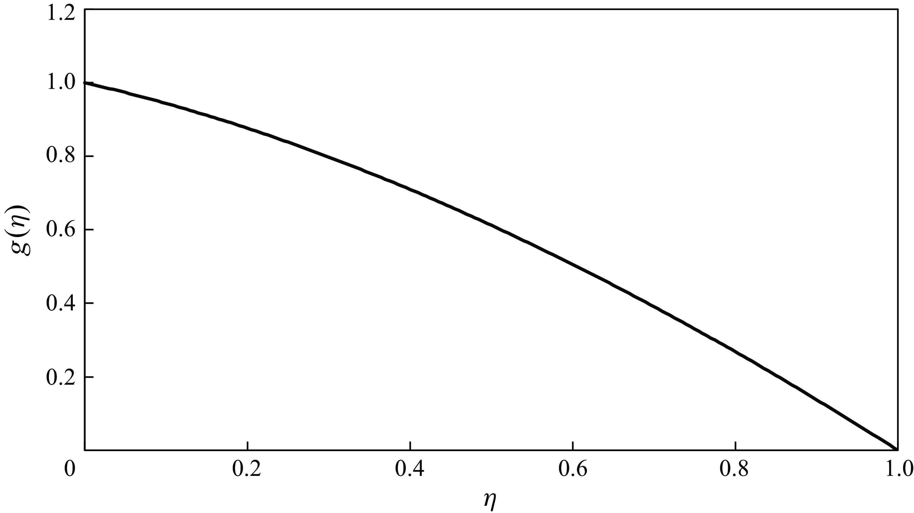
 \begin{equation} g(\eta ) = \big [ (1 - \eta )(1 - \eta ^2 )\big ]^{1/2}. \end{equation}
The self-similar solution (2.9) of the interface profile
 $g(\eta )$
in the low-permeability layer in an unconfined porous medium with negligible motion of the ambient fluid.

The function
 $g(\eta )$
is plotted in figure 2, which highlights the nonlinear nature of the interface profile between the invading and displaced fluids. By using (2.8) along with the solution curve presented in figure 2, the dimensional values of the thickness profile at any time
 $t$
may be obtained.
We are also interested in finding the total amount of injecting fluid that invades into each layer of the unconfined porous strata during constant pressure injection. The total volume of fluid
 $V_1$
in the high-permeability layer is computed straightforwardly using (2.2) as
 \begin{equation} V_1(t) = \phi _1 w\, x_f(t) \equiv \left (\frac {2k_1\, \Delta p_1}{\mu }\right )^{1/2} \phi _1 w \,t^{1/2}, \end{equation}
for a unit thickness in the third dimension. The total volume of fluid
 $V_2$
that leaks into the low-permeability layer can be computed by integrating (2.5) between
 $x=0$
and
 $x=x_{f}(t)$
as follows:
 \begin{equation} V_2(t) = \phi _2 \int _{0}^{x_f(t)} h(x,t) \,\textrm {d}x = \frac {2(16\sqrt {2} - 14)}{15}\frac { \Delta p_1\, (k_1 k_2)^{1/2}}{\mu } \phi _2 \,t, \end{equation}
for a unit thickness in the third dimension. Equations (2.10) and (2.11) together give us the ratio of volumes in each layer as a function of time:
 \begin{equation} \frac {V_1(t)}{V_2(t)} = \frac {15}{2(16\sqrt {2} - 14)} \left (\frac {\mu }{\Delta p_1\, k_2}\right )^{1/2} \frac {\phi _1}{\phi _2} w \,t^{-1/2}. \end{equation}
Note that (2.12) simply represents
 $V_1/V_2 \propto w/h_0(t)$
, the ratio of the two length scales perpendicular to the primary flow direction, since the profile thickness in the low-permeability layer follows
 $h_0(t) \propto (k_2\, \Delta p_1\, t/\mu )^{1/2}$
based on (2.8). This result is physically plausible because the length scales in the primary flow direction along the channel are the same in both the high- and low-permeability layers. The
 $t^{-1/2}$
dependence in (2.12) indicates that at large times, most fluid would be leaked into the low-permeability layer when
 $h_0(t) \gg w$
.
3. Laboratory experiments
Schematic of the experimental set-up: (a) side view, (b) top view.

We performed laboratory experiments with the aim of verifying some of the findings of § 2. Experiments were performed in a transparent acrylic tank filled with spherical glass beads. The tank was saturated with salt water as the ambient fluid, while the glycerine–water mixture was used as the viscous injecting fluid. We considered injection pressure and fluid viscosity as experimental variables. A dye attenuation technique was used for flow visualisation, where experimental images were post-processed in Matlab to extract the fluid–fluid interface profile.
3.1. Experimental set-up
A transparent acrylic rectangular tank of dimensions 78 cm long
 $\times$
20 cm wide
 $\times$
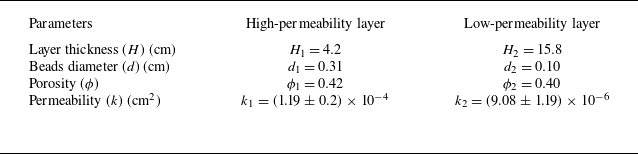
1 cm height was used in these laboratory experiments, as depicted in figure 3. The tank was filled with spherical glass beads of diameters 0.31 cm and 0.1 cm to make two porous layers of different permeabilities. To be consistent with the description of the theoretical model, the experiments with two permeability layers (and not three) are symmetric across the transverse direction. The high-permeability layer with larger beads was 4.2 cm in thickness, and the low-permeability layer with smaller beads was 15.8 cm in thickness. The porosity of the porous layers was measured experimentally, whereas the permeability of the layers was estimated using the well-accepted Kozeny–Carman equation for spherical beads:
 \begin{equation} k = \frac {d^2 \phi ^3}{180 (1-\phi )^2}, \end{equation}
where
 $d$
is the bead diameter, and
 $\phi$
is the porosity. Such a treatment has been shown to be reliable (e.g. Acton et al. Reference Acton, Huppert and Worster2001). The measured porosity and permeability values for both layers are detailed in table 1. For the two beads layers, we obtained
 $k_1 = (1.19 \pm 0.2) \times 10^{-4}$
cm
 $^2$
and
 $k_2 = (9.08 \pm 1.19) \times 10^{-6}$
cm
 $^2$
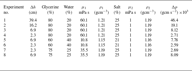
, respectively. The complete tank was saturated with salt water of varying density (
 $\rho _2$
) and viscosity (
 $\mu _2 = 1$
mPa s). For these experiments, the glycerine–water mixture was used as the more-viscous fluid for injection whose viscosity (
 $\mu _1$
) and density (
 $\rho _1$
) depend on the mixture composition. In a typical experiment, we have
 $\mu _1 \in [10.8,60.1]$
mPa s and
 $\rho _1 \in [1.15,1.21]$
g cm
 $^{-3}$
. The values of the ambient and injecting fluid properties are listed in table 2 for various experiments.
Details of the permeable layers used in the experiments.

Details of the experiments performed: subscript 1 indicates injecting fluid, subscript 2 indicates ambient fluid.

As shown in figure 3, the viscous fluid was injected into the tank at the high-permeability layer through an inlet port, which was located at
 $x = 0$
cm and
 $y = 0$
cm, and had area approximately 0.2 cm
 $^2$
. The viscous fluid was supplied from an overhead tank that generated injection pressure for the inflow into the experimental tank. Both the overhead tank and the outlet of the experimental tank were open to the atmosphere. Moreover, during an experimental run, the water level in the overhead tank was maintained constant using an overflow hole. Thus the elevation difference
 $\Delta h$
between the overhead tank and experimental tank outlet created a constant hydrostatic pressure difference
 $\Delta p = (\rho _1 - \rho _a)g\, \Delta h$
for the flow during each experiment. The elevation of the overhead tank was varied for different sets of experiments. By changing the glycerine–water composition to achieve different viscosities, and the overhead tank elevation for various pressure differences, we performed a total of eight experiments. The associated details are listed in table 2.
Sample of experimental images for the temporal evolution of the interface profile in Exp-2 from table 2 at different times: (a)
 $t = 0$
s, (b)
 $t = 144$
s, (c)
 $t = 252$
s, and (d)
 $t = 504$
s. The black curves represent the fluid–fluid interface and are detected using the algorithm presented in Appendix C. The field of view for each image measures 78 cm long
 $\times$
20 cm wide. The two permeability layers (and not three) are symmetric across the transverse direction.

(a) Exp-1 at
 $t = 217$
s, with
 $\Delta h= 39.4$
cm and
 $\mu _2 / \mu _1= 60.1$
. (b) Exp-3 at
 $t = 756$
s, with
 $\Delta h= 6.9$
cm and
 $\mu _2 / \mu _1= 60.1$
. (c) Exp-6 at
 $t = 420$
s, with
 $\Delta h= 2.3$
cm and
 $\mu _2 / \mu _1= 10.8$
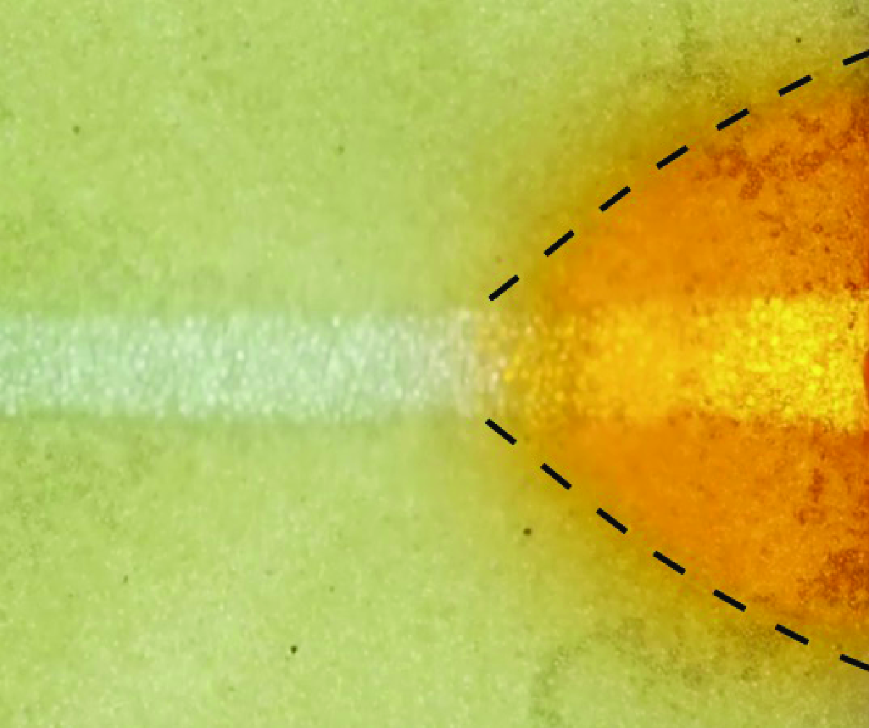
. The two permeability layers (and not three) are symmetric across the transverse direction. We typically observed the development of a tail in the high-permeability layer in these experiments, and the length of the tail is influenced significantly by the viscosity ratio.

For flow visualisation, a red-coloured food dye was added to the glycerine–water mixture before injection, while the less-viscous ambient fluid was kept transparent. During experiments, a Nikon D5000 DSLR camera with resolution
 $4288\times2848$
pixels was used to capture images of the flow, and an LED light panel of the same size as that of the experimental tank was placed underneath the tank for illumination to capture sharp and better images. The experimental room was kept dark from other possible light sources except the LED light panel. We collected images at intervals of approximately 36 s for most of the experiments. Depending on the duration of the experiments, which lasted between 10 and 30 minutes, approximately 50–100 images were captured for each experiment.
3.2. Qualitative observation
Figure 4 shows the time evolution of the propagating front
 $x_f(t)$
and thickness profile
 $h_f(x, t)$
using the solid black lines in different panels for a sample experiment. The junction of two permeable layers is highlighted using a dashed blue line. In the high-permeability layer, we observe that the viscous fluid flows with different rates between the layers’ junction and the lower tank wall. This stretches the propagating front longitudinally, which might be occurring because of either (i) a thick high-permeability medium, which is assumed to be very thin in the theoretical model, which allows leakage on only one side, or (ii) improper packing of beads towards the lower wall such that at the boundary, the permeability is relatively higher, resulting into local heterogeneity (see inset of figure 4
a). In contrast, the theoretical solution is derived considering a very thin high-permeability medium, such that flow remains predominantly one-dimensional.
Therefore, to make a sensible comparison, we consider the location of propagating front at the centreline in the high-permeability layer marked by a purple dashed line in figure 4. The location of the propagating front is marked by a vertical dashed blue line. It may be of interest to note that the influence of heterogeneity perpendicular to the flow direction has been discussed in the context of viscous gravity current (e.g. Huppert & Woods Reference Huppert and Woods1995; Zheng et al. Reference Zheng, Soh, Huppert and Stone2013; Hinton & Woods Reference Hinton and Woods2018), unsaturated flow (e.g. Zheng Reference Zheng2022) and particle dispersion (e.g. Hinton & Woods Reference Hinton and Woods2019).
(a) Experimental observations of the propagating front location
 $x_f(t)$
versus time
 $t$
. (b) A log-log plot illustrating dimensionless forms. Theoretical predictions are also included as the curves for comparison. Early time data are shown in the inset in (a).

(a) Experimental observations of the propagating maximum thickness
 $h(0,t)$
versus time
 $t$
. (b) A log-log plot illustrating dimensionless forms. Theoretical predictions are also included as the curves for comparison. Early time data are shown in the inset in (a).

To understand more about the stretched tail in the high-permeability layer, we show in figure 5 the interface profiles for various experiments to qualitatively compare the effects of experimental parameters. For example, Exp-3 in figure 5(b) shows a reasonably flat front that is the closest to the theoretical model, in contrast to the large stretch shown by Exp-6 in figure 5(c). Note that the details of the experiments are given in table 2, where Exp-3 has viscosity ratio approximately 60, but Exp-6 has ratio only approximately 10. Furthermore, while Exp-1 in figure 5(a) has the advantage of a high viscosity ratio, the pressure difference is very large compared to that for Exp-3. Overall, we observe least longitudinal stretching of the propagating front for the more-viscous fluid with less pressure difference. Both these factors result in low Reynolds number of the flow. As the theoretical model is explicitly derived using Darcy’s law for low Reynolds number cases, the experimental observations of figure 5 are consistent with the theoretical assumptions.
3.3. Quantitative analysis
In this subsection, we compare the experimental measurement of this section with the theoretical results obtained in § 2. In particular, we compare the location of the propagating front in the high-permeability layer and the thickness profile of the fluid–fluid interface in the low-permeability layer. In particular, the length and thickness of the invading fluid are both small compared with the size of the packed-bead tank at early times, and the displacement can be considered as unconfined. In contrast, the influence of the motion of the ambient fluid could become more important at late times, and applying the confined model is likely more appropriate.
For a comparison between the theoretical predictions and experimental observations for the location of the propagating front in the high-permeability layer, the calculated permeability
 $k_1$
is used. For the thickness prediction in the low-permeability layer, the calculated permeability
 $k_2$
is used. Both
 $k_1$
and
 $k_2$
are provided in table 1. The pressure difference
 $\Delta p_1$
needed in the theoretical model, e.g. in (A4) and (A11), is obtained from table 2. The total pressure difference
 $\Delta p$
from table 2 is subtracted from the pressure drop due to friction loss in the pipe network used before the fluid enters the porous media tank, thus the actual inlet pressure is
 $\Delta p_1 = \Delta p_{ai}$
. The calculations for pressure losses and the actual inlet pressure
 $p_{ai}$
are presented in Appendix B.
In figures 6(a) and 7(a), we present a comparison between the theoretical and experimental results for the frontal location
 $x_f(t)$
and inlet thickness
 $h(0,t)$
versus time
 $t$
. For both
 $x_f(t)$
and
 $h(0,t)$
, we see good agreement for some of the experiments, and significant deviations for the others, depending on the experimental variables.
In figures 6(b) and 7(b), we plot
 $x_f(t)$
and
 $h(0,t)$
in the log-log scale based on their non-dimensionalised values in the forms
 \begin{equation} \hat {x}_f = x_f(t)/x_f(t_{max}) \end{equation}
and
 \begin{equation} \hat {h} = h(0,t)/h(0,t_{max}), \end{equation}
together with
 \begin{equation} \hat {t} = t/t_{max}, \end{equation}
where
 $t_{max}$
is the last time when an image is captured in each experiment. Further, we also included the theoretical predictions based on the unconfined flow model. We find good agreement between the theory and experimental data for both
 $x_f(t)$
and
 $h(0,t)$
at intermediate times, as shown in figures 6 and 7, respectively. We see that the slopes of the theoretical models match closely with the slope exhibited by the experimental data as well. These results validate the existence of the scaling exponent
 $1/2$
.
Normalised interface profile of fluid–fluid interface with respect to maximum values
 $h(0,t_{max})$
of thickness profile at
 $x=0$
and front location
 $x_f(t_{max})$
at the final time
 $t_{max}$
for each experiment. The solid curve represents the prediction of an unconfined medium.

In figure 8, we present a comparison for the interface profile
 $h(x,t_{max})$
of the invading fluid that has leaked into the low-permeability medium at the final time
 $t_{max}$
. Figure 8 is normalised using
 $x_f(t_{max})$
and
 $h(0,t_{max})$
for individual experiments, so that all experiments can be compared together. The theoretical thickness profile is also plotted for the unconfined model, as predicted by (2.8), which shows reasonable agreement with the normalised experimental data. This agreement is consistent with what we have observed in figure 6 for the propagating front in the high-permeability layer and thickness profile at
 $x=0$
in the low-permeability layer. Moreover, the comparison here indicates a mismatch of the total fluid volume between theory and experiments. Presumably, this is due to the existence of the faster region ahead of
 $x_f(t_{max})$
, which is not accounted for in the theory. In experiments with higher viscosity ratio, the mismatch is less significant.
3.4. Final remarks
To summarise, when we compare the theoretical predictions with the experimental observations, we find that the normalised profile shapes at different times collapse reasonably well onto a universal curve for the low Reynolds number cases, and this universal profile shape agrees well with the prediction of the theory. For the frontal location, which is defined as the fluid front at the centreline of the high-permeability layer for the experiments, the power-law scaling exponent is also well captured by the theory at intermediate times. Nevertheless, we have also observed that the prefactors could be different by up to 20 % for the low Reynolds number cases, and the difference becomes even more significant (by up to 60 %) for cases of higher Reynolds number. Such a disagreement becomes more clear in figure 9 when we compare the original theoretically predicted and experimentally measured profile shapes at different times, compared with the comparison in normalised plots such as figure 8. For the high Reynolds number cases Exp-6 and Exp-7, the comparison becomes even worse. Our current understanding is that this is due primarily to the existence of the stretched tail of the injecting fluid in the high-permeability layer, which is related to the boundary effects at the wall and impermeable packing, as well as the fact that injection is through a point source rather a line source across the high-permeability layer in the experiments. Overall, we consider that the simple theory well captured some major trends of the experimental observations.
Comparison between theoretically predicted and experimentally measured profiles of the leaked fluid in the low-permeability layer at different times and in representative experiments: (a) Exp-1, and (b) Exp-2. The primary reason for the disagreement comes from prediction of the frontal location. Here,
 $L$
and
 $H$
denote the length and thickness of the low-permeability layer, respectively.

However, we do recognise the disagreement between the theoretical prediction and the experimental observation, in particular, on the generation of the tail in the high-permeability layer and hence the value of the prefactor in the frontal law. To obtain more insights, we have performed new experiments in a three-layer packed-bead system, where two low-permeability layers are created and attach to a narrow high-permeability layer at the centre. Details of the new experiments can be found in the supplementary material. In these additional experiments, we have also allowed the boundary at
 $y=H$
to be either permeable or impermeable, to evaluate its influence. In either case, we have observed that the tail could be significantly suppressed in the high-permeability layer, allowing fluid leakage on both sides of the high-permeability layer. This is particularly true when the high-permeability layer is set narrower. Meanwhile, we have observed that when the far-field boundary is made permeable at
 $y=H$
in the experiments, the simple one-dimensional model provides much better predictions for both the profile shape evolution and the frontal locations. In contrast, when the far-field boundary is made impermeable at
 $y=H$
, the prediction of the one-dimensional simple theory could become invalid for the profile shape evolution of the leaked fluid at intermediate times.
4. Summary and conclusions
Leakage and flow of contaminants through high-permeability channels like fractures and faults in the subsurface are common. These leakages possibly result in contamination and often environmental risks. We have investigated in this work the displacement flow of a less-viscous fluid by a more-viscous fluid in a layered porous medium having a large permeability jump between the layers, a typical situation of natural porous rocks. The study comprises both theoretical predictions and experimental observations. The results from our study may be used to model such flows and estimate the amount of leakage through single high-permeability channels. The theoretical and experimental results may also be of use to validate numerical models to study such flows under more realistic boundary and injection conditions.
In particular, we first developed a theoretical model to predict the time evolution of the longitudinal and transverse profiles of the injecting viscous fluid. While the viscous fluid propagates along the high-permeability layer, it gradually leaks into the low-permeability medium transversely. With time, it builds a larger thickness near the injection point, which slowly narrows towards the propagating front. Our theoretical model arrives at a self-similar solution for the thickness profile when the flow is unconfined, with a frontal propagation law
 $x_f(t) \propto t^{1/2}$
in the high-permeability layer. We also found that the volume ratio of the fluid that flows through the high-permeability channel to leaks into the low-permeability layers follows a
 $V_1/V_2 \propto t^{-1/2}$
power law with time. In contrast, for confined flows, self-similar behaviour is not expected due to the associated length scales.
The experimental set-up consisted of two layers of different permeabilities, using two different sizes of spherical glass beads. The working fluids were fresh water as the ambient fluid, and glycerine–water mixtures as the injecting more-viscous fluid. The experimental measurements validate the prediction of the front propagation law
 $x_f(t) \propto t^{1/2}$
and the volume ratio
 $V_1/V_2 \propto t^{-1/2}$
. The comparison between experimental and theoretical results shows a better agreement for the experiments with larger viscosity differences and at smaller Reynolds numbers under low-pressure injections, which mimics most underground/subsurface flows.
We also recognise the limitations posed by our experimental set-up, e.g. having a thick high-permeability medium, and with a limited size of the tank. Also, the far-field boundary is sealed rather than being left permeable to allow transverse flow. All these features are inconsistent with a key assumption of the simple theory that the flow in the low-permeability layer is one-dimensional in the transverse direction. This inconsistency becomes particularly important at late times, when the fluid–fluid interface gets close to the boundary, and the flow must become longitudinal. Correspondingly, when we compare our experimental observations with the theoretical predictions, we have observed that while the power-law scaling exponent seems well captured, there exists also a notable difference for the prefactors of the frontal location at intermediate times. Such a difference is typically up to 20 % for experiments performed at low Reynolds numbers, and it could become even more significant (up to 60 %) for higher Reynolds number cases. Finally, the additional experiments performed in a three-layer symmetric system, as described in the supplementary material, provide useful insights into the influence of impermeable/permeable far-field boundary conditions.
In the future, we plan to expand this study to explore a wider range of permeability ratios between the high- and low-permeability layers, and the viscosity differences between the invading and ambient fluids. In particular, it could be of use to study the typically unstable flow situations, when a less-viscous fluid invades a more-viscous ambient fluid. In this case, buoyancy could possibly suppress the development of the viscous fingering instability, and enforce the injected fluid to propagate as a gravity current, so it is also of interest to study the intermediate regime between viscous fingering and gravity current. We could also consider increasing the relative size of the tank, such that
 $H$
and
 $L$
are much greater than the typical length and height of the interface profiles, respectively, so the flow could be considered more appropriately as one-dimensional, as assumed in the model. Furthermore, investigating the effects of gravity/buoyancy on such flows may put further insights into more realistic scenarios.
Supplementary material
Supplementary material is available at https://doi.org/10.1017/jfm.2025.10242.
Acknowledgements
C.K.S. and Z.Z. would like to thank M. Bickle and J.A. Neufeld for helpful earlier discussions. The experiments were performed at the University of Cambridge.
Funding
Z.Z. acknowledges partial support by the Program for Professor of Special Appointment (Eastern Scholar, no. TP2020009) at Shanghai Institutions of Higher Learning.
Declaration of interests
The authors report no conflict of interest.
Appendix A. A confined model of non-zero viscosity ratio
Schematic of fluid displacement and leakage in a confined porous medium. The system is of length
 $L$
and includes a high-permeability layer of width
 $w$
, and two low-permeability layers of width
 $H$
. The interface
 $h(x,t)$
between the invading and displaced fluids is shown by the red curve and described by a confined solution (A12). Motion of the displaced fluid is now considered that is perpendicular to the direction of the high-permeability channel.

In contrast to the unconfined model of zero viscosity ratio, as presented in § 2.1, here we consider a confined model that accounts for the motion of the ambient fluid as a result of viscous displacement by the injecting fluid. As a result, the viscosity ratio becomes relevant in the model and solutions due to the confined nature of the flow. Again, we constrain our discussions in the sharp-interface limit when the influence of fluids mixing is negligible.
A schematic of the model problem is given in figure 10. The viscosity of the injecting fluid is greater than that of the ambient fluid, i.e.
 $\mu _1 \gt \mu _2$
. For simplicity, we again neglect the influence of the wetting and capillary effects, and assume that no significant instability develops at the time scale of interest. While we account for the pressure variation in the ambient fluid now, we assume the outer boundary of the medium to be sufficiently far that the ambient pressure at the boundary is constant, i.e.
 $p(x,y,t)=p_a$
at
 $x = L$
, and
 $y = \pm w/2 + H$
. The pressure at any location
 $x$
in the high-permeability layer is denoted by
 $p_x(x,t)$
, and pressure at the fluid–fluid interface in the high- and low-permeability layers is denoted by
 $p_f(t)$
and
 $p_h(x,t)$
, respectively.
We first investigate the fluid motion within the high-permeability layer, which has total flow domain length
 $L$
. Darcy’s law for the one-dimensional flows of the invading and displaced fluids yields
 \begin{equation} \frac {\textrm {d} x_f}{\textrm {d} t} = \frac {k_1}{\mu _1}\,\frac {p_i - p_f(t)}{x_f} \end{equation}
and
 \begin{equation} \frac {\textrm {d} x_f}{\textrm {d} t} = \frac {k_1}{\mu _2}\,\frac {p_f(t) - p_a}{L - x_f}. \end{equation}
Rearranging (A1) and (A2), and using the initial condition that
 $x_f(0)=0$
, we obtain an algebraic equation for the front location
 $x_f(t)$
:
 \begin{equation} \Delta \mu\, {x_f^2(t)} + 2\mu _2 L\, x_f(t) - 2k_1\, \Delta p_1\, t = 0, \end{equation}
where
 $\Delta \mu = \mu _1 - \mu _2 \gt 0$
. We also recall that
 $\Delta p_1 = p_i - p_a \gt 0$
represents the imposed pressure difference. For the quadratic equation derived in (A3), we obtain an analytical expression for
 $x_f(t)$
as
 \begin{equation} x_f(t) = \frac {-\mu _2 L + (\mu _2^2 L^2 +2k_1\, \Delta \mu\, \Delta p_1\, t)^{1/2}}{\Delta \mu }. \end{equation}
We note that (A4) now accounts for the motion of the displaced fluid. There is also the assumption that the top boundary must be permeable, otherwise the flow of the ambient fluid would become two-dimensional at intermediate times rather than being one-dimensional (and perpendicular to the direction of the high-permeability channel). This is more consistent with the new experiments as presented in the supplementary material rather than those in the main text with impermeable boundaries. In addition, (A4) recovers the diffusive behaviour of (2.2) when
 $\mu _2 \rightarrow 0$
, and also when
 $t \gg (\Delta \mu\, {x_f^2(t)}) /(2k_1\, \Delta \mu\, \Delta p_1)$
, i.e. when the pressure loss from the motion of the displaced fluid is negligible compared with the imposed pressure difference
 $\Delta p_1$
.
The pressure distribution in the high-permeability layer decreases linearly along the
 $x$
direction at leading order in both
 $x \in [0,x_f(t)]$
and
 $x \in [x_f(t),L]$
, but with different slopes that depend on the viscosity of the flowing fluid. Nevertheless, we can also compute the pressure at the front
 $p_f(t)$
in the high-permeability layer at any time
 $t$
based on
 \begin{equation} p_f(t) = \frac {\mu _2[L-x_f(t)]p_i +\mu _1\, x_f(t)\, p_a}{\mu _1\, x_f(t) + \mu _2[L-x_f(t)]}, \end{equation}
and the pressure distribution along the
 $x$
direction in the high-permeability layer at any location
 $x \in [0,x_f(t)]$
and time
 $t$
by
 \begin{equation} p_x(x,t) = \frac {p_i[x_f(t) - x] + p_f(t)\, x}{x_f(t)}. \end{equation}
Next, we estimate the transverse fluid leakage into the low-permeability layer. For finding the velocity, we use the difference in pressure between the high-permeability layer, i.e.
 $p_x(x,t)$
, and the fluid–fluid interface, denoted by
 $p_h(x,t)$
. We assume that there is no pressure jump across the interface, such that the velocities of the invading and displaced fluids, respectively, are
 \begin{equation} \frac {\partial h(x,t)}{\partial t} = \frac {k_2}{\mu _1}\,\frac {p_x(x,t) - p_h(x,t)}{h(x,t)} \end{equation}
and
 \begin{equation} \frac {\partial h(x,t)}{\partial t} = \frac {k_2}{\mu _2}\,\frac {p_h(x,t) - p_a}{H - h(x,t)}. \end{equation}
(a) A log-log plot of the propagating frontal location
 $x_f(t)$
versus time
 $t$
in dimensionless forms. (b) A log-log plot of the propagating maximum thickness
 $h_0(t)$
versus time
 $t$
in dimensionless forms. Theoretical predictions of both the unconfined and confined models are also included as the solid lines, for comparison.

Here,
 $H$
is the width of the low-permeability layer. Equations (A7) and (A8) can be rearranged and integrated to provide an algebraic equation for the interface profile
 $h(x,t)$
as
 \begin{equation} \Delta \mu\, {h^2(x,t)} + 2\mu _2 H\,h(x,t) - f_0(x,t)\,(t-t_0(x)) = 0, \end{equation}
where the function
 $f_0(x,t)$
and the time lag
 $t_0(x)$
are given by
 \begin{equation} f_0(x,t) = 2k_2[p_x(x,t) - p_a] \end{equation}
and
 \begin{equation} t_0(x) = \frac {\Delta \mu \, x^2 + 2\mu _2 {L\, x}}{2k_1\, \Delta p_1}. \end{equation}
The algebraic equation (A9) provides a unique positive solution for the interface thickness
 $h(x,t)$
as
 \begin{equation} {h(x,t) = \frac {-\mu _2 {H} + [\mu _2^2 H^2 + \Delta \mu\, f_0(x,t)\,(t-t_0(x))]^{1/2}}{\Delta \mu }.} \end{equation}
We see that (A12) now accounts for the effect of the displaced fluid motion in the low-permeability layers. As can be double checked, as
 $\mu _2 \rightarrow 0$
, (A12) recovers (2.5) when the motion of the displaced fluid is negligible. In contrast to (2.5), (A12) does not result in a similarity solution because of the associated length scale
 $H$
. It is also seen that the confined model provides a first-order correction in terms of the viscosity ratio
 $\mu _2/\mu _1$
to the unconfined model. In other words, the unconfined model is the zero-viscosity-ratio limit of the confined model presented here, for better interpretability of the modelling efforts.
We are also interested in finding the total amount of injecting fluid that invades into each layer of the confined porous strata during constant pressure injection. The total volume of fluid
 $V_{1c}$
in the high-permeability layer is computed straightforwardly using (A4) as
 \begin{equation} V_{1c}(t) = \phi _1 w\, x_f(t) = \phi _1 w \frac {-\mu _2 L + (\mu _2^2 L^2 +2k_1\, \Delta \mu\, \Delta p_1\, t)^{1/2}}{\Delta \mu } \end{equation}
for a unit thickness in the third dimension. The total volume of fluid
 $V_{2c}$
that leaks into the low-permeability layer can be computed by integrating (A12) between
 $0$
and
 $x_{f}(t)$
as follows:
 \begin{align} V_{2c}(t) &= \phi _2 \int _{0}^{x_f(t)} h(x,t) \,\textrm {d}x \nonumber\\ &= \phi _2 \int _{0}^{x_f(t)} {\frac {-\mu _2 {H} + \left[\mu _2^2 H^2 + \Delta \mu\, f_0(x,t)\,(t-t_0(x))\right ]^{1/2}}{\Delta \mu } \,\textrm {d}x} \end{align}
for a unit thickness in the third dimension.
Before we close this appendix, we now provide more calculations to evaluate how the unconfined and confined models work. In figures 11(a) and 11(b), we include experimental data for both
 $x_f(t)$
and
 $h(0,t)$
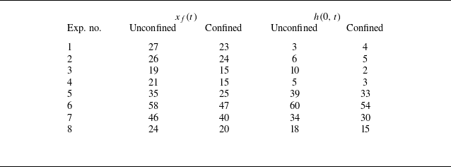
in dimensionless forms, and we also include predictions of both the unconfined and confined models. We see good agreement for some of the experiments, and significant deviations for the others, depending on the experimental variables. These comparisons are quantified by calculating mean errors between the theory and experiments. To find the mean errors, we first find absolute errors between the theory and experiments at various times, then we average these values to find the mean error for the given experiment. The mean errors for both
 $x_f(t)$
and
 $h(0,t)$
are listed in table 3 for all experiments. We observe that the lowest mean errors are obtained for experiments with the highest viscosity and lowest pressure difference, i.e. Exp-2 to Exp-4.
Presented mean error % for
 $x_f(t)$
and
 $h(0,t)$
comparison with theory results based on the late-time data points when
 $t/t_{max} \in [1/2,1]$
as displayed in figures 11(a,b).

In figure 12, we also present a comparison for the normalised interface profile
 $h(x,t_{max})$
of the invading fluid that has leaked into the low-permeability medium at the final time
 $t_{max}$
. The theoretical thickness profiles are also included for both the unconfined and confined models, as predicted by (2.8) and (A12), respectively. We see slight differences between the theoretical profiles of the unconfined and confined models, and they both result in over-prediction. The profiles of the confined model show better agreement with the experiments, particularly for the cases involving the injection of a more-viscous fluid, e.g. for Exp-1 to Exp-4. However, we must also note that since the side wall of the cell is sealed at
 $y=H$
rather than being permeable, which indicates non-negligible two-dimensional flow effects in particular when the fluid–fluid interface is close to the side wall and limits the applicability of the confined model as well.
Normalised interface profile of the fluid–fluid interface with respect to maximum values
 $h(0,t_{max})$
of the thickness profile at
 $x=0$
and front location
 $x_f(t_{max})$
at the final time
 $t_{max}$
for each experiment. The solid curves represent the theoretical predictions for confined media for various viscosity used in the experiments, whereas the dashed curves show the predictions for an unconfined medium.

Appendix B. Frictional losses in the inlet pipe
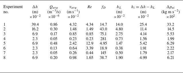
For our experiments, the pressure difference between the inlet and outlet of the experimental tank worked as a major variable. To use an accurate value of the pressure difference for comparison between theory and experiments, we subtract the head loss that occurred in the inlet pipe network from the value obtained between the overhead tank and experimental tank outlet. In table 4, we provide the details of miscellaneous parameters that we use for finding the head losses through the pipe.
Head loss due to friction in the inlet pipe for each experiment.

To calculate the fluid velocity through the pipe, we first find the volume of the injecting fluid in the experimental tank at various times by measuring the areas of the contaminated regions in the high- and low-permeability layers separately using image processing. We then adjust the measured volumes for their pore volumes as follows:
 \begin{equation} V_t = A_t^1 W_T \phi _1 + A_t^2 W_T \phi _2, \end{equation}
where
 $A_t^1$
and
 $A_t^2$
are the contaminated areas in the high- and low-permeability media, respectively, and
 $\phi _1$
and
 $\phi _2$
are their porosities. Moreover,
 $W_T=1$
cm is the depth of the medium. This volume is then used to find the volume flux through the system:
 \begin{equation} Q_t = \frac {V_{t_2} - V_{t_1}}{t_2 - t_1} \end{equation}
and
 \begin{equation} Q_{avg} = \frac {Q_t}{N}, \end{equation}
where
 $N$
is defined as the number of images under consideration in each experiment. Finally, the average velocity through the pipe over the course of an experiment is
 \begin{equation} v_{avg} = Q_{avg}/A_i, \end{equation}
where
 $A_i$
is the pipe cross-section for the diameter
 $d_i=0.5\ \rm cm$
.
Further, we find the Reynolds number of the flow through the inlet pipe as
 \begin{equation} Re = \frac {\rho _0 v_{avg} {d}_i}{\mu _0}, \end{equation}
which measures as
 $Re\lt 2000$
for all experiments. As the flow is in a laminar regime, we find the head loss using the Darcy–Weisbach friction factor such that
 \begin{equation} f_D = \frac {64}{Re} \end{equation}
and hence
 \begin{equation} h_L = \frac {f_D L_p (v_{avg})^2}{2 g {d}_i}, \end{equation}
where
 $L_p= 50\ \rm cm$
is the length of the inlet pipe. The head loss
 $h_L$
calculated is subsequently subtracted from the pressure head
 $\Delta h$
, originally given in table 2. Actual inlet pressure is calculated as
 $\Delta p_{ai} = (\rho _1-\rho _a) g h_i$
.
Appendix C. Further remarks on post-processing
Comparison of propagating front location
 $x_f(t)$
at the centreline of the high-permeability layer and at the junction of the two layers versus time
 $t$
with the theory of the confined model.

Images captured during experiments were post-processed in Matlab to detect the location of the propagating front in the high-permeability layer and the thickness profile in the low-permeability layer. First, all experimental images were cropped to retain only the region of interest, as shown in figure 4. Then a reference image, which was taken just before starting each experiment, i.e. figure 4(a), was used to subtract the experimental images taken at time
 $t \gt 0$
, i.e. figures 4(b–d). The subtraction created a resultant image with zero light intensity for the ambient fluid. Subsequently, contours were drawn to separate the viscous fluid from the less-viscous fluid using threshold value 1 % of the maximum intensity in the image. These contours produced the location of the propagating front and fluid–fluid interface, as highlighted by black contours in figure 4.
In figure 13, the theoretical prediction for the location of the propagating front is compared with the experimental values both at the centreline (circles) and at the interface of the two packed-bead layers (triangles). We see a better agreement with the centreline values, which seems justifiable as it includes the boundary effects in the measurements. For all further analysis in the present work, we consider only the centreline values for the location of the propagating front. Recall that generation of the tail in the high-permeability bead layer seems a major difference from the assumption of the simple model, and this is likely due to the boundary effects at the impermeable wall, and also the mixing of the two permeable layers of different bead sizes at the junction.
Appendix D. Evolution of the volume ratio
Finally, in figure 14, we compare the fluid volumes
 $V_1(t)/V_2(t)$
within the high- and low-permeability layers. Again, we found in the log-log plot that the
 $t^{-1/2}$
scaling law appears, which is consistent with the prediction (2.12) of the unconfined theory. However, there is also non-negligible disagreement with regard to the prefactor in solution (2.12), similar to what we have observed when analysing the experimental data on the frontal propagation law
 $x_f(t)$
and the inlet thickness evolution
 $h(0,t)$
, as discussed in the main text. The difference is likely due to other effects, such as the boundary effects at the wall and also two-dimensional flow effects that are not considered by the simple one-dimensional model. Notice that the influence of the mixing bead layer is already accounted for here to generate this figure by shifting the interface of the two bead layers by 2 mm towards the low-permeability layer in the transverse direction. Without doing this, the disagreement regarding the prefactor is even more significant.
Experimental observations of the volume ratio
 $V_1/V_2$
versus time
 $t$
, and the theoretical predictions are also included as the curves for comparison. We observe good agreement for the power-law scaling, while there exist differences for the prefactors.