1 Introduction
The issue of noise generation from aerofoils has been the subject of much theoretical, experimental and computational research over the past few decades and is of great importance in many applications, such as jet engines, wind turbine blades, high-speed propellers, helicopter blades, etc. Aerofoil noise can generally be categorized as self-noise and inflow-turbulence interaction noise. The aerofoil self-noise is due to the interaction of the aerofoil with its own boundary layer and the flow instabilities present in the boundary layer (Brooks, Pope & Marcolini Reference Brooks, Pope and Marcolini1989). The aerofoil inflow-turbulence interaction noise, on the other hand, is due to the interaction of an incoming unsteady gust with the aerofoil. The aerofoil inflow-turbulence interaction noise is a significant contributor in systems involving multiple rows of blades, such as jet engines and contra-rotating propellers. For instance, the wake flow shed by the aircraft engine fan blades interacts with following blades and vanes, causing leading-edge noise from the rear blades. Likewise, the interaction of the wake flow from the front row blades in a contra-rotating open rotor (CROR) system with the downstream blades is considered as the main source of broadband noise from such configurations. Also, the interaction of atmospheric turbulence with the blades of wind turbines can similarly cause high levels of low-frequency broadband noise.
The prediction of aerofoil inflow-turbulence interaction noise has been the subject of much research over the past few decades (Sears Reference Sears1941; Graham Reference Graham1970; Amiet Reference Amiet1975; Devenport, Staubs & Glegg Reference Devenport, Staubs and Glegg2010). Sears originally considered the interaction of an unsteady sinusoidal gust with a flat plate and developed a model for the prediction of the plate aerodynamic response under such unsteady loading. Sears’ model was later further developed and extended to compressible flows by Graham (Reference Graham1970) and Amiet (Reference Amiet1975). In Amiet’s model, the blade response function to an incoming gust is first obtained using the Schwarzschild technique and the far-field sound is then formulated based on the theories of Kirchoff and Curle (Reference Curle1955) using the radiation integral. Amiet’s model shows that the far-field sound power spectral density (PSD) is directly related to the energy spectrum of the velocity fluctuations of the incoming gust. It has been widely shown that Amiet’s model can provide fairly good comparisons with experimental observations when the turbulence statistical quantities are known. The effects of aerofoil geometrical parameters, such as angle of attack, aerofoil thickness, camber, etc. on the generation of leading-edge turbulence interaction noise has also been the subject of some theoretical studies (Goldstein & Atassi Reference Goldstein and Atassi1976; Goldstein Reference Goldstein1978; Atassi, Fang & Patrick Reference Atassi, Fang and Patrick1993; Myers & Kerschen Reference Myers and Kerschen1995, Reference Myers and Kerschen1997; Devenport et al. Reference Devenport, Staubs and Glegg2010; Roger & Carazo Reference Roger and Carazo2010).
The use of leading-edge treatments, inspired by the flippers of humpback whales (Bushnell & Moore Reference Bushnell and Moore1991; Fish & Battle Reference Fish and Battle1995; Miklosovic & Murray Reference Miklosovic and Murray2004; Fish, Howle & Murray Reference Fish, Howle and Murray2008; Pedro & Kobayashi Reference Pedro and Kobayashi2008), has been shown to lead to improved aerodynamic and hydrodynamic performance, particularly at high angles of attack. The recent extensive experimental work on the effects of leading-edge serrations on the generation and control of turbulence interaction noise has shown that the use of such treatments can result in significant noise reduction over a wide range of frequencies (Hansen, Kelso & Doolan Reference Hansen, Kelso and Doolan2012; Narayanan et al. Reference Narayanan, Chaitanya, Haeri, Joseph, Kim and Placsek2015). For example, Narayanan et al. (Reference Narayanan, Chaitanya, Haeri, Joseph, Kim and Placsek2015) showed that using sinusoidal leading-edge serrations for a flat plate and NACA-65 type aerofoil leads to significant noise reduction. Noise reduction was found to be significantly greater for the flat plates. It was also shown that the sound power reduction level is more sensitive to the serration amplitude and less sensitive to the serration wavelength. In a more recent study, it was shown that the use of complex leading-edge serrations, i.e. serrations formed from the superposition of two serration profiles of different frequency, amplitude and phase, can produce greater noise reduction than single wavelength serrations (Chaitanya et al. Reference Chaitanya, Narayanan, Joseph and Kim2016).
Besides the experimental activities, the problem of aerofoil inflow-turbulence interaction noise reduction using wavy edges has recently been investigated in several computational studies (Lau, Haeri & Kim Reference Lau, Haeri and Kim2013; Kim, Haeri & Joseph Reference Kim, Haeri and Joseph2016; Turner & Kim Reference Turner and Kim2016). In the work of Lau et al. (Reference Lau, Haeri and Kim2013), the effectiveness of leading-edge serrations for turbulence interaction noise reduction was examined numerically. It was found that the hydrodynamic quantity
 $k_{1}h$
plays an important role in determining the effectiveness of the serration, where
 $k_{1}$
is the hydrodynamic wavenumber of the disturbance in the streamwise direction and the serration root-to-tip distance is
 $2h$
. The serration wavelength
 $\unicode[STIX]{x1D706}$
, on the other hand, was found to be less important. However, one should note that the study assumed a perfect coherence in the spanwise direction, which may not be the case in real-world applications. The three-dimensionality of the disturbance was accounted for in the work of Kim et al. (Reference Kim, Haeri and Joseph2016) using synthetically generated turbulence. It was argued that both a source cut-off and destructive interference effects contributed to the sound reduction. Both of these two numerical studies used a regular sinusoidal serration profile attached to a flat plate. In a more recent study by Turner & Kim (Reference Turner and Kim2016), a dual-frequency wavy serration profile was proposed and it was found that the more complex serration geometries can increase noise reduction. It is again worth noting that the upstream disturbance was assumed to be perfectly correlated in the spanwise direction.
The above discussion provides a comprehensive literature review of the use of leading-edge serrations as a passive method for the reduction of aerofoil inflow-turbulence interaction noise. It is, however, worth mentioning that the topic of using leading-edge serrations for improving the aerodynamic performance of aerofoils has attracted much attention over the past few decades. A great many experimental and numerical studies have been conducted to investigate the effects of leading-edge modifications on aerofoil aerodynamic forces, early separation and stall behaviour, unsteady forces, etc., at different flow regimes. The detailed literature review of the aerodynamic performance of serrated aerofoils is beyond the scope of this study, but interested readers can refer to some of the very first activities (Soderman Reference Soderman1972) and more recent research (Miklosovic & Murray Reference Miklosovic and Murray2004; Johari et al. Reference Johari, Henoch, Custodio and Levshin2007; Hansen, Kelso & Dally Reference Hansen, Kelso and Dally2011), where detailed literature reviews and comprehensive studies are provided.
Despite the significant body of work on noise reduction using leading-edge serrations, no mathematical model has yet been developed to relate the radiated noise to the serration geometrical parameters and turbulence quantities. While the experimental observations (Paterson & Amiet Reference Paterson and Amiet1976; Roger & Carazo Reference Roger and Carazo2010; Roger, Schram & Santana Reference Roger, Schram and Santana2013; Narayanan et al. Reference Narayanan, Chaitanya, Haeri, Joseph, Kim and Placsek2015) and computational studies (Atassi et al. Reference Atassi, Fang and Patrick1993; Hixon et al. Reference Hixon, Mankbadi, Scott, Sawyer and Nallasamy2006; Allampalli et al. Reference Allampalli, Hixon, Nallasamy and Sawyer2009; Gill, Zhang & Joseph Reference Gill, Zhang and Joseph2013; Lau et al. Reference Lau, Haeri and Kim2013; Kim et al. Reference Kim, Haeri and Joseph2016; Turner & Kim Reference Turner and Kim2016) have provided the evidence that leading-edge serrations can lead to significant noise reduction, an accurate and robust analytical model can help in better understanding the mechanism of such noise reductions. An accurate analytical model will also enable us to assess the effectiveness of leading-edge serrations at high Mach numbers and Reynolds numbers, relevant to turbomachinery applications, where numerical approaches are costly and experiments difficult. This will also provide us with a tool for blade-design optimization purposes. In this paper, we aim to extend Amiet’s leading-edge noise-prediction model to the case of serrated leading edges and provide a parametric study of the effects of serrations on far-field noise. It will be shown in § 2 that the introduction of serrations will lead to a complex differential equation, which is solved using the Schwarzschild technique in an iterative manner. The scattered pressure loading will then be used in a radiation integral and the far-field PSD will be found in terms of the incoming gust statistical quantities and blade response function. Section 3 presents an extensive parametric study of the proposed model and results will be provided for far-field sound pressure level (SPL), noise directivity and overall SPL. The noise-reduction mechanism will also be discussed in this section. Section 5 concludes the paper and lists our future plans.
2 Analytical formulation
In this section, we present a detailed derivation for the prediction of noise due to the interaction of an unsteady gust with a flat plate with a serrated leading edge. The analytical model developed is based on Amiet’s model and the Schwarzschild technique for solving the Helmholtz equation with appropriate boundary conditions.
2.1 Leading-edge noise modelling
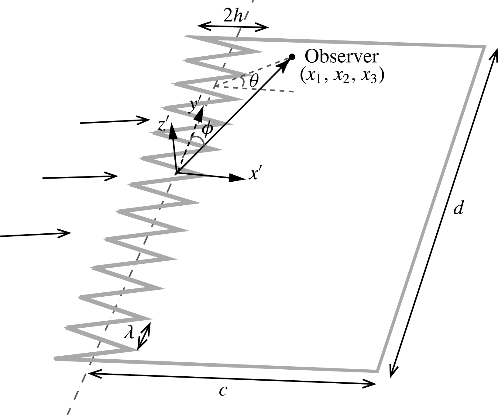
Let us consider an infinitesimally thin flat plate with leading-edge serrations, as shown in figure 1, with an averaged chord length
 $c$
and spanwise length
 $d$
. A Cartesian coordinate system is chosen such that the serration profile is an oscillatory function of zero mean. When the acoustic wavelength is smaller than the chord length
 $c$
, the flat plate can be considered as an infinitely long plate without a trailing edge (Amiet Reference Amiet1976b
, Reference Amiet1978; Roger & Moreau Reference Roger and Moreau2005). When the frequencies are high enough such that the semi-infinite simplification is permissible, the plate can also be considered infinite in the spanwise direction when it has a relatively large aspect ratio, typically larger than 3 (Amiet Reference Amiet1978; Roger & Carazo Reference Roger and Carazo2010). Let
 $x^{\prime }$
,
 $y^{\prime }$
and
 $z^{\prime }$
denote the streamwise, spanwise and normal directions to the plate, respectively. The observer point is located at
 $(x_{1},x_{2},x_{3})$
, as shown in figure 1.
Schematic of a flat plate with a sawtooth-like leading edge.

As mentioned above, the origin of the coordinate system (
 $x^{\prime },y^{\prime },z^{\prime }$
) is chosen such that the serration profile,
 $H(y^{\prime })$
, is an oscillatory function of zero mean and that
 $H(y^{\prime })=0$
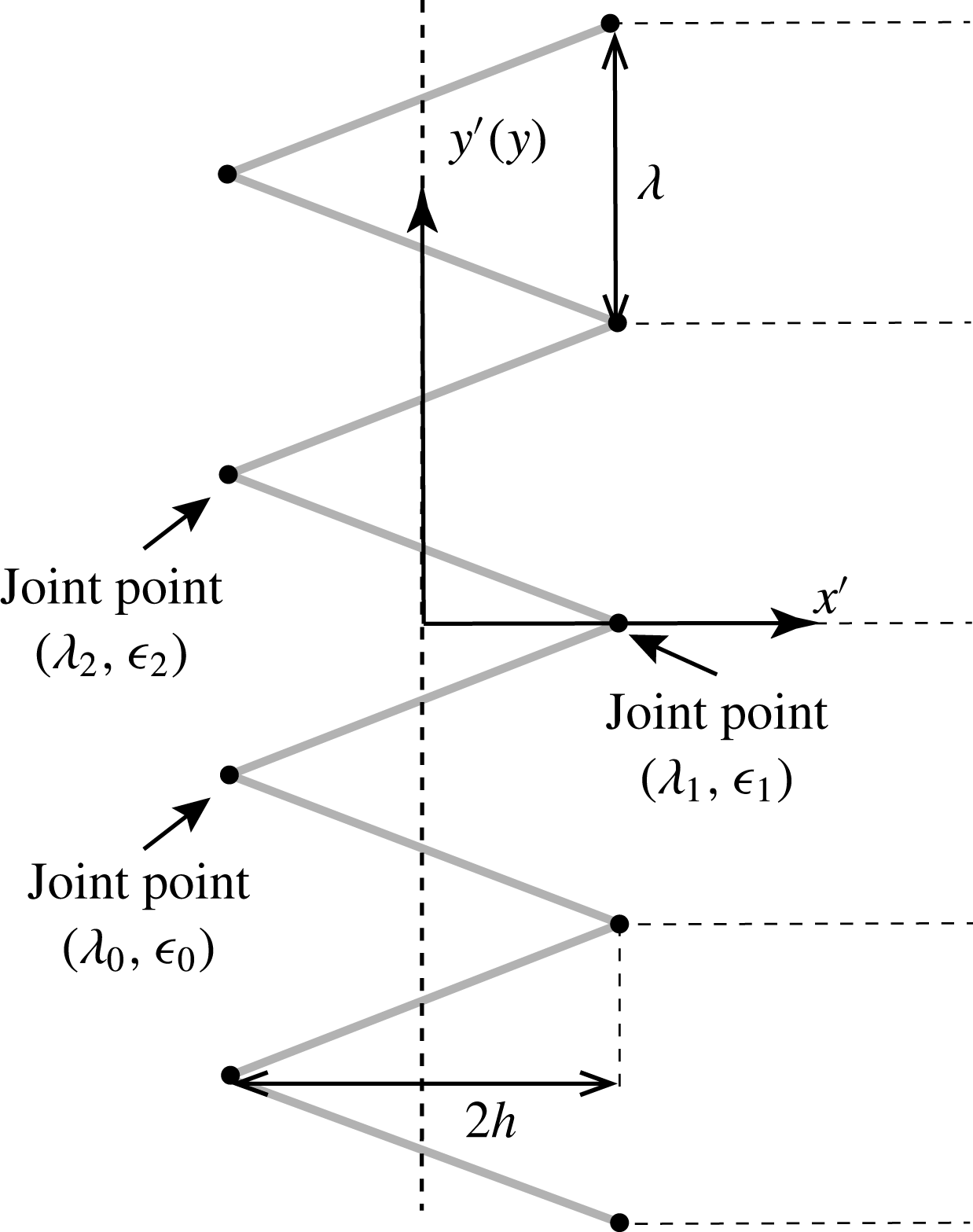
in the absence of serrations. Though the method developed in this section can be used for any general periodic serrations, in this paper we only focus on the sawtooth serration, as shown in figure 1, where the root-to-tip length is
 $2h$
and the serration wavelength is
 $\unicode[STIX]{x1D706}$
. The parameter
 $\unicode[STIX]{x1D70E}=4h/\unicode[STIX]{x1D706}$
will also be used to quantify the sharpness of the sawtooth serrations. To obtain a mathematical description of
 $H(y^{\prime })$
, let us consider a single sawtooth centred on the coordinate origin and let
 $(\unicode[STIX]{x1D706}_{0},\unicode[STIX]{x1D716}_{0})$
,
 $(\unicode[STIX]{x1D706}_{1},\unicode[STIX]{x1D716}_{1})$
and
 $(\unicode[STIX]{x1D706}_{2},\unicode[STIX]{x1D716}_{2})$
denote the three joint-points defining this single sawtooth, as shown in figure 2. The serration profile function
 $H(y^{\prime })$
can therefore be defined as
 $$\begin{eqnarray}H(y^{\prime })=\left\{\begin{array}{@{}ll@{}}\unicode[STIX]{x1D70E}_{0}(y^{\prime }-\unicode[STIX]{x1D706}_{0}-m\unicode[STIX]{x1D706})+\unicode[STIX]{x1D716}_{0},\quad & \unicode[STIX]{x1D706}_{0}+m\unicode[STIX]{x1D706}<y^{\prime }\leqslant \unicode[STIX]{x1D706}_{1}+m\unicode[STIX]{x1D706}\\ \unicode[STIX]{x1D70E}_{1}(y^{\prime }-\unicode[STIX]{x1D706}_{1}-m\unicode[STIX]{x1D706})+\unicode[STIX]{x1D716}_{1},\quad & \unicode[STIX]{x1D706}_{1}+m\unicode[STIX]{x1D706}<y^{\prime }\leqslant \unicode[STIX]{x1D706}_{2}+m\unicode[STIX]{x1D706},\end{array}\right.\end{eqnarray}$$
where
 $\unicode[STIX]{x1D70E}_{j}=(\unicode[STIX]{x1D716}_{j+1}-\unicode[STIX]{x1D716}_{j})/(\unicode[STIX]{x1D706}_{j+1}-\unicode[STIX]{x1D706}_{j})$
,
 $j=0,1$
and
 $m=0$
,
 $\pm 1,\pm 2,\pm 3\cdots \,$
.
A schematic of the serration profile.

In this paper, we focus our attention on the unsteady upwash disturbance (Amiet Reference Amiet1975), denoted by
 $w$
, that exists upstream of the leading edge, convecting downstream with the mean flow at a speed of
 $U$
. According to Kovasznay (Reference Kovasznay1953), the unsteady motion on a uniform flow can be decomposed into vorticity, entropy and sound-wave modes. When perturbation amplitudes are small such that linearization is permissible, the three modes can be considered mutually independent. It is generally accepted that the incident turbulence can be well represented by the vorticity mode, which convects at the speed of the mean flow. Therefore, this study follows the same simplification and the incoming gust is assumed to be frozen in the frame moving with the mean flow, i.e. the velocity distribution is
 $w(x^{\prime },y^{\prime },t)=w_{m}(x^{\prime }-Ut,y^{\prime })$
, where
 $t$
denotes time, for some function
 $w_{m}(x_{m},y_{m})$
describing the distribution of upwash velocity in the travelling coordinate system
 $\{x_{m},y_{m},z_{m}\}$
. In the plate fixed frame, the incoming gust can be written in terms of its wavenumber components,
 $\tilde{w}(k_{1},k_{2})$
, as
 $$\begin{eqnarray}w(x^{\prime },y^{\prime },t)=\iint _{-\infty }^{\infty }\tilde{w}(k_{1},k_{2})\text{e}^{\text{i}(k_{1}(x^{\prime }-Ut)+k_{2}y^{\prime })}\,\text{d}k_{1}\,\text{d}k_{2},\end{eqnarray}$$
where the Fourier component
 $\tilde{w}(k_{1},k_{2})$
is given by
 $$\begin{eqnarray}\tilde{w}(k_{1},k_{2})=\left({\displaystyle \frac{1}{2\unicode[STIX]{x03C0}}}\right)^{2}\iint _{-L}^{L}w_{m}(x_{m},y_{m})\text{e}^{-\text{i}(k_{1}x_{m}+k_{2}y_{m})}\,\text{d}x_{m}\,\text{d}y_{m},\end{eqnarray}$$
where
 $L$
is a large but finite number to avoid convergence difficulties and
 $k_{1}$
and
 $k_{2}$
denote the Fourier wavenumbers in the streamwise and spanwise directions, respectively. Using (2.2) one can find
 $$\begin{eqnarray}\displaystyle w(x^{\prime },y^{\prime },\unicode[STIX]{x1D714}) & = & \displaystyle {\displaystyle \frac{1}{2\unicode[STIX]{x03C0}}}\int w(x^{\prime },y^{\prime },t)\text{e}^{\text{i}\unicode[STIX]{x1D714}t}\,\text{d}t\nonumber\\ \displaystyle & = & \displaystyle {\displaystyle \frac{1}{U}}\int _{-\infty }^{\infty }\tilde{w}(\unicode[STIX]{x1D714}/U,k_{2})\text{e}^{\text{i}(\unicode[STIX]{x1D714}x^{\prime }/U+k_{2}y^{\prime })}\,\text{d}k_{2},\end{eqnarray}$$
where
 $\unicode[STIX]{x1D714}$
represents angular frequency.
Equation (2.4) suggests that a general unsteady gust can be decomposed into a set of plane-wave-like gusts, each of which takes the form of
 $$\begin{eqnarray}w_{i}=w_{ia}\text{e}^{-\text{i}(\unicode[STIX]{x1D714}t-k_{1}x^{\prime }-k_{2}y^{\prime })},\end{eqnarray}$$
where
 $k_{1}=\unicode[STIX]{x1D714}/U$
and
 $w_{ia}$
denotes the magnitude of the upwash velocity and is a function of both
 $\unicode[STIX]{x1D714}$
and
 $k_{2}$
. The scattered velocity potential
 $\unicode[STIX]{x1D719}_{t}$
is governed by the convective wave equation, i.e.
 $$\begin{eqnarray}\unicode[STIX]{x1D6FB}^{2}\unicode[STIX]{x1D719}_{t}-{\displaystyle \frac{1}{c_{0}^{2}}}\left({\displaystyle \frac{\unicode[STIX]{x2202}}{\unicode[STIX]{x2202}t}}+U{\displaystyle \frac{\unicode[STIX]{x2202}}{\unicode[STIX]{x2202}x^{\prime }}}\right)^{2}\unicode[STIX]{x1D719}_{t}=0,\end{eqnarray}$$
where
 $c_{0}$
denotes the speed of sound. Hence, if we can find the far-field sound induced by a single gust by solving the wave equation subject to appropriate boundary conditions upstream of the leading edge and over the surface of the serrated plate, then a more general solution can readily be obtained by performing an integration over
 $k_{2}$
, as shown in (2.4). The next part of this section is therefore devoted to the single-gust solution for a flat plate with sawtooth leading-edge serrations.
2.2 Single-gust solution
The full solution
 $\unicode[STIX]{x1D719}_{t}$
to (2.6) can be written in terms of an initial and a residual potential part. The initial potential,
 $\unicode[STIX]{x1D719}_{i}$
, is used to cancel the upwash velocity on the plane
 $z^{\prime }=0$
. Upon defining
 $k=\unicode[STIX]{x1D714}/c_{0}$
,
 $\unicode[STIX]{x1D6FD}^{2}=1-M_{0}^{2}$
and
 $M_{0}=U/c_{0}$
, one can show that on the plane
 $z^{\prime }=0$
,
 $\unicode[STIX]{x1D719}_{i}$
takes the form of
 $$\begin{eqnarray}\unicode[STIX]{x1D719}_{i}=-\unicode[STIX]{x1D6F7}_{ia}\text{e}^{-\text{i}(\unicode[STIX]{x1D714}t-k_{1}x^{\prime }-k_{2}y^{\prime })},\end{eqnarray}$$
where
 $\unicode[STIX]{x1D6F7}_{ia}\equiv -w_{ia}/\sqrt{(k_{1}\unicode[STIX]{x1D6FD}+kM_{0}/\unicode[STIX]{x1D6FD})^{2}+k_{2}^{2}-(k/\unicode[STIX]{x1D6FD})^{2}}$
.
The Schwarzschild technique can then be used to calculate the second part, i.e. residual term, of the potential field,
 $\unicode[STIX]{x1D719}$
, which would cancel the potential field of the initial solution upstream of the leading edge (such that we have
 $\unicode[STIX]{x1D719}_{t}=0$
for
 $x^{\prime }<0$
and
 $z^{\prime }=0$
). Thus, the boundary conditions at
 $z^{\prime }=0$
for
 $\unicode[STIX]{x1D719}$
read
 $$\begin{eqnarray}\left.\begin{array}{@{}ll@{}}{\displaystyle \frac{\unicode[STIX]{x2202}\unicode[STIX]{x1D719}}{\unicode[STIX]{x2202}z^{\prime }}}=0, & x^{\prime }>H(y^{\prime })\\ \unicode[STIX]{x1D719}=\unicode[STIX]{x1D6F7}_{ia}\text{e}^{-\text{i}(\unicode[STIX]{x1D714}t-k_{1}x^{\prime }-k_{2}y^{\prime })}, & x^{\prime }\leqslant H(y^{\prime }).\end{array}\right\}\end{eqnarray}$$
The equation governing the second-part potential field
 $\unicode[STIX]{x1D719}$
remains unchanged, i.e.
 $$\begin{eqnarray}\unicode[STIX]{x1D6FB}^{2}\unicode[STIX]{x1D719}-{\displaystyle \frac{1}{c_{0}^{2}}}\left({\displaystyle \frac{\unicode[STIX]{x2202}}{\unicode[STIX]{x2202}t}}+U{\displaystyle \frac{\unicode[STIX]{x2202}}{\unicode[STIX]{x2202}x^{\prime }}}\right)^{2}\unicode[STIX]{x1D719}=0.\end{eqnarray}$$
Equation (2.9) together with the boundary conditions given in (2.8) forms a well-posed mathematical problem and we attempt to solve it in this section.
2.2.1 Boundary-value problem
With the assumption of harmonic perturbation
 $\unicode[STIX]{x1D719}=\unicode[STIX]{x1D6F7}(x^{\prime },y^{\prime },z^{\prime })\text{e}^{-\text{i}\unicode[STIX]{x1D714}t}$
, equation (2.9) reduces to
 $$\begin{eqnarray}\unicode[STIX]{x1D6FD}^{2}{\displaystyle \frac{\unicode[STIX]{x2202}^{2}\unicode[STIX]{x1D6F7}}{\unicode[STIX]{x2202}x^{\prime 2}}}+{\displaystyle \frac{\unicode[STIX]{x2202}^{2}\unicode[STIX]{x1D6F7}}{\unicode[STIX]{x2202}z^{\prime 2}}}+{\displaystyle \frac{\unicode[STIX]{x2202}^{2}\unicode[STIX]{x1D6F7}}{\unicode[STIX]{x2202}y^{\prime 2}}}+2\text{i}kM_{0}{\displaystyle \frac{\unicode[STIX]{x2202}\unicode[STIX]{x1D6F7}}{\unicode[STIX]{x2202}x^{\prime }}}+k^{2}\unicode[STIX]{x1D6F7}=0.\end{eqnarray}$$
In order to make the boundary conditions in (2.8) independent of
 $y^{\prime }$
, the coordinate transformation
 $x=x^{\prime }-H(y^{\prime }),y=y^{\prime },z=z^{\prime }$
is used (Roger et al.
Reference Roger, Schram and Santana2013), which leads to the following differential equation (Sinayoko, Azarpeyvand & Lyu Reference Sinayoko, Azarpeyvand and Lyu2014; Lyu, Azarpeyvand & Sinayoko Reference Lyu, Azarpeyvand and Sinayoko2015, Reference Lyu, Azarpeyvand and Sinayoko2016a
):
 $$\begin{eqnarray}(\unicode[STIX]{x1D6FD}^{2}+{H^{\prime }}^{2}(y)){\displaystyle \frac{\unicode[STIX]{x2202}^{2}\unicode[STIX]{x1D6F7}}{\unicode[STIX]{x2202}x^{2}}}+{\displaystyle \frac{\unicode[STIX]{x2202}^{2}\unicode[STIX]{x1D6F7}}{\unicode[STIX]{x2202}y^{2}}}+{\displaystyle \frac{\unicode[STIX]{x2202}^{2}\unicode[STIX]{x1D6F7}}{\unicode[STIX]{x2202}z^{2}}}-2H^{\prime }(y){\displaystyle \frac{\unicode[STIX]{x2202}^{2}\unicode[STIX]{x1D6F7}}{\unicode[STIX]{x2202}x\unicode[STIX]{x2202}y}}+(2\text{i}M_{0}k-H^{\prime \prime }(y)){\displaystyle \frac{\unicode[STIX]{x2202}\unicode[STIX]{x1D6F7}}{\unicode[STIX]{x2202}x}}+k^{2}\unicode[STIX]{x1D6F7}=0,\end{eqnarray}$$
where
 $H^{\prime }(y)$
and
 $H^{\prime \prime }(y)$
denote the first and second derivatives of
 $H(y)$
with respect to
 $y$
. The boundary conditions now read
 $$\begin{eqnarray}\left.\begin{array}{@{}ll@{}}\unicode[STIX]{x1D6F7}(x,y,0)=\unicode[STIX]{x1D6F7}_{ia}\text{e}^{\text{i}(k_{1}x+k_{2}y)}\text{e}^{\text{i}k_{1}H(y)}, & x\leqslant 0\\ \unicode[STIX]{x2202}\unicode[STIX]{x1D6F7}(x,y,0)/\unicode[STIX]{x2202}z=0, & x>0.\\ \end{array}\right\}\end{eqnarray}$$
The set of equations (2.11) and (2.12) forms a linear boundary-value problem. However, unlike the governing equation for a straight leading edge (Amiet Reference Amiet1976a
), the coefficients in (2.11) now depend on
 $y$
and therefore the standard ‘separation of variables’ technique cannot be easily applied. Therefore, a Fourier expansion technique will be initially employed to eliminate the
 $y$
dependency in (2.11), as explained in the following section.
2.2.2 Fourier expansion
Using both the infinite-span and serration periodicity assumptions, one can make use of the Fourier series in terms of the new coordinates (
 $x,y,z$
) to expand the induced potential due to the gust interaction as
 $$\begin{eqnarray}\unicode[STIX]{x1D6F7}(x,y,z)=\mathop{\sum }_{-\infty }^{\infty }\unicode[STIX]{x1D6F7}_{n}(x,z)\text{e}^{\text{i}k_{2n}y},\end{eqnarray}$$
where
 $k_{2n}=k_{2}+2n\unicode[STIX]{x03C0}/\unicode[STIX]{x1D706}$
. Substituting this expansion into (2.11) and multiplying the resulting equation by
 $\text{e}^{-\text{i}k_{2n^{\prime }}y}$
, then integrating over
 $y$
from
 $-\unicode[STIX]{x1D706}/2$
to
 $\unicode[STIX]{x1D706}/2$
, one can readily show that
 $$\begin{eqnarray}\displaystyle & & \displaystyle \left\{\unicode[STIX]{x1D6FD}^{2}{\displaystyle \frac{\unicode[STIX]{x2202}^{2}}{\unicode[STIX]{x2202}x^{2}}}+{\displaystyle \frac{\unicode[STIX]{x2202}^{2}}{\unicode[STIX]{x2202}z^{2}}}+2\text{i}kM_{0}{\displaystyle \frac{\unicode[STIX]{x2202}}{\unicode[STIX]{x2202}x}}+(k^{2}-k_{2n^{\prime }}^{2})\right\}\unicode[STIX]{x1D6F7}_{n^{\prime }}\nonumber\\ \displaystyle & & \displaystyle \qquad +\,{\displaystyle \frac{1}{\unicode[STIX]{x1D706}}}\int _{-\unicode[STIX]{x1D706}/2}^{\unicode[STIX]{x1D706}/2}\mathop{\sum }_{n=-\infty }^{\infty }\left\{H^{\prime 2}{\displaystyle \frac{\unicode[STIX]{x2202}^{2}}{\unicode[STIX]{x2202}x^{2}}}-(H^{\prime \prime }+2\text{i}k_{2n}H^{\prime }){\displaystyle \frac{\unicode[STIX]{x2202}}{\unicode[STIX]{x2202}x}}\right\}\unicode[STIX]{x1D6F7}_{n}\text{e}^{\text{i}(2(n-n^{\prime })\unicode[STIX]{x03C0}/\unicode[STIX]{x1D706})y}\,\text{d}y=0.\qquad\end{eqnarray}$$
If both
 $H^{\prime }(y)$
and
 $H^{\prime \prime }(y)$
were constant within the entire wavelength, the summation over different modes in (2.14) would vanish and one would obtain an equation which only involves one mode, say
 $n^{\prime }$
. However, for the profile of the sawtooth serration,
 $H^{\prime }(y)$
, is not continuous and hence
 $H^{\prime \prime }(y)$
is singular at the joint-points (
 $\unicode[STIX]{x1D706}_{i},\unicode[STIX]{x1D716}_{i}$
). We use the generalized function
 $\unicode[STIX]{x1D6FF}(y)$
to describe the singularities, i.e.
 $$\begin{eqnarray}\left.\begin{array}{@{}c@{}}\displaystyle H^{\prime }(y)=\left\{\begin{array}{@{}ll@{}}\unicode[STIX]{x1D70E}_{0},\quad & \unicode[STIX]{x1D706}_{0}+m\unicode[STIX]{x1D706}<y\leqslant \unicode[STIX]{x1D706}_{1}+m\unicode[STIX]{x1D706}\\ \unicode[STIX]{x1D70E}_{1},\quad & \unicode[STIX]{x1D706}_{1}+m\unicode[STIX]{x1D706}<y\leqslant \unicode[STIX]{x1D706}_{2}+m\unicode[STIX]{x1D706},\\ \quad \end{array}\right.\\ \displaystyle H^{\prime \prime }(y)=\mathop{\sum }_{m=-\infty }^{\infty }(-1)^{m+1}2\unicode[STIX]{x1D70E}\unicode[STIX]{x1D6FF}(x-m\unicode[STIX]{x1D706}/2),\end{array}\right\}\end{eqnarray}$$
where
 $\unicode[STIX]{x1D70E}=4h/\unicode[STIX]{x1D706}$
signifies the serration sharpness. As
 $\int _{-\infty }^{\infty }\unicode[STIX]{x1D6FF}(x)f(x)\,\text{d}x=f(0)$
, the summation in (2.14) cannot be dropped, indicating that different modes are coupled together. Substituting the serration profile function and its derivatives, equation (2.1) and (2.15), into (2.14) and making use of the fact that
 $\int _{-\infty }^{\infty }f(x)\unicode[STIX]{x1D6FF}(x-\unicode[STIX]{x1D70F})\,\text{d}x=f(\unicode[STIX]{x1D70F})$
, we obtain
 $$\begin{eqnarray}\displaystyle & & \displaystyle \left\{(\unicode[STIX]{x1D6FD}^{2}+\unicode[STIX]{x1D70E}^{2}){\displaystyle \frac{\unicode[STIX]{x2202}^{2}}{\unicode[STIX]{x2202}x^{2}}}+{\displaystyle \frac{\unicode[STIX]{x2202}^{2}}{\unicode[STIX]{x2202}z^{2}}}+2\text{i}kM_{0}{\displaystyle \frac{\unicode[STIX]{x2202}}{\unicode[STIX]{x2202}x}}+(k^{2}-k_{2n^{\prime }}^{2})\right\}\unicode[STIX]{x1D6F7}_{n^{\prime }}\nonumber\\ \displaystyle & & \displaystyle \qquad =-{\displaystyle \frac{4\unicode[STIX]{x1D70E}}{\unicode[STIX]{x1D706}}}\mathop{\sum }_{n-n^{\prime }=\mathit{odd}}\left(1-{\displaystyle \frac{k_{2}\unicode[STIX]{x1D706}+2n\unicode[STIX]{x03C0}}{(n-n^{\prime })\unicode[STIX]{x03C0}}}\right){\displaystyle \frac{\unicode[STIX]{x2202}\unicode[STIX]{x1D6F7}_{n}}{\unicode[STIX]{x2202}x}}.\end{eqnarray}$$
We can write the set of differential equations obtained above in a more compact matrix form. Using a linear operator
 $$\begin{eqnarray}{\mathcal{D}}=\left\{(\unicode[STIX]{x1D6FD}^{2}+\unicode[STIX]{x1D70E}^{2}){\displaystyle \frac{\unicode[STIX]{x2202}^{2}}{\unicode[STIX]{x2202}x^{2}}}+{\displaystyle \frac{\unicode[STIX]{x2202}^{2}}{\unicode[STIX]{x2202}z^{2}}}+2\text{i}kM_{0}{\displaystyle \frac{\unicode[STIX]{x2202}}{\unicode[STIX]{x2202}x}}\right\},\end{eqnarray}$$
and a vector of functions
 $$\begin{eqnarray}\unicode[STIX]{x1D731}=\left(\cdots \unicode[STIX]{x1D6F7}_{-n^{\prime }}(x,z),\unicode[STIX]{x1D6F7}_{-n^{\prime }+1}(x,z),\ldots \unicode[STIX]{x1D6F7}_{n^{\prime }-1}(x,z),\unicode[STIX]{x1D6F7}_{n^{\prime }}(x,z),\ldots \right)^{\text{T}},\end{eqnarray}$$
the coupled equations in (2.16) can be written as
 $$\begin{eqnarray}{\mathcal{D}}\unicode[STIX]{x1D731}=\unicode[STIX]{x1D63C}\unicode[STIX]{x1D731}+\unicode[STIX]{x1D63D}{\displaystyle \frac{\unicode[STIX]{x2202}\unicode[STIX]{x1D731}}{\unicode[STIX]{x2202}x}},\end{eqnarray}$$
where the symbol
 $\text{T}$
in (2.18) denotes the transpose of a matrix. Matrices
 $\unicode[STIX]{x1D63C}$
and
 $\unicode[STIX]{x1D63D}$
denote the coefficient matrices of
 $\unicode[STIX]{x1D731}$
and
 $\unicode[STIX]{x2202}\unicode[STIX]{x1D731}/\unicode[STIX]{x2202}x$
, respectively, and the elements
 $A_{ml}$
and
 $B_{ml}$
, representing the entry corresponding to mode
 $m$
in row and
 $l$
in column of matrices
 $\unicode[STIX]{x1D63C}$
and
 $\unicode[STIX]{x1D63D}$
, are given by
 $$\begin{eqnarray}A_{ml}=(k_{2m}^{2}-k^{2})\unicode[STIX]{x1D6FF}_{ml},\quad B_{ml}=\left\{\begin{array}{@{}ll@{}}{\displaystyle \frac{4\unicode[STIX]{x1D70E}}{\unicode[STIX]{x1D706}}}{\displaystyle \frac{m+l+k_{2}\unicode[STIX]{x1D706}/\unicode[STIX]{x03C0}}{l-m}},\quad & m-l=\text{odd}\\ 0,\quad & m-l=\text{even},\end{array}\right.\end{eqnarray}$$
where
 $\unicode[STIX]{x1D6FF}_{ml}$
represents the Kronecker delta.
The boundary condition for each mode
 $n$
can be obtained by substituting the profile geometry, (2.1), into the boundary conditions, (2.12), and performing the same Fourier expansions:
 $$\begin{eqnarray}\left.\begin{array}{@{}ll@{}}\unicode[STIX]{x1D6F7}_{n}(x,0)=\unicode[STIX]{x1D6F7}_{ia}a_{n}\text{e}^{\text{i}k_{1}x}, & x\leqslant 0\\ {\displaystyle \frac{\unicode[STIX]{x2202}\unicode[STIX]{x1D6F7}_{n}}{\unicode[STIX]{x2202}z}}(x,0)=0, & x>0,\end{array}\right\}\end{eqnarray}$$
where
 $a_{n}$
is defined as
 $$\begin{eqnarray}a_{n}={\displaystyle \frac{1}{\unicode[STIX]{x1D706}}}\int _{-\unicode[STIX]{x1D706}/2}^{\unicode[STIX]{x1D706}/2}\text{e}^{\text{i}k_{1}H(y)}\text{e}^{-\text{i}(2n\unicode[STIX]{x03C0}/\unicode[STIX]{x1D706})y}\,\text{d}y.\end{eqnarray}$$
Before we attempt to solve (2.19), it is worth examining some of its important properties. Matrix
 $\unicode[STIX]{x1D63C}$
is obviously a diagonal matrix and if
 $\unicode[STIX]{x1D63D}$
was also diagonal, we would be able to solve each mode individually, i.e. no mode coupling. However,
 $\unicode[STIX]{x1D63D}$
is not a diagonal matrix and different modes are coupled together, in the sense that
 $\unicode[STIX]{x1D6F7}_{n}$
, for example, appears in the governing equation of
 $\unicode[STIX]{x1D6F7}_{m}$
. This means that every mode is interacting with the other modes and cannot be solved individually. Also, it can be observed from the expression of
 $\unicode[STIX]{x1D63D}$
in (2.20) that the strength of the mode coupling is proportional to
 $\unicode[STIX]{x1D70E}/\unicode[STIX]{x1D706}$
. This indicates that mode coupling becomes stronger for sharper serrations. Obviously, the mode-coupling phenomenon fades away when the serration amplitude
 $2h$
is very small and the solution is reduced to that of Amiet’s model for a straight leading edge. Also, at very low frequencies it is expected that the contribution of higher-order modes becomes negligible compared with the zero mode. Thus, for the equation governing the zero mode, the coupling with higher modes becomes weak. One can, therefore, solve the zero mode individually and calculate the potential with only the contribution of the zero mode. But this only works for very low frequencies or for very wide serrations. The coupling effect becomes more pronounced at high frequencies. To solve these coupled equations at relatively high frequencies we will use an iterative procedure, which is explained in the following section.
2.2.3 Induced potential field
To obtain the induced potential field, equation (2.19) together with the boundary conditions in (2.21) needs to be solved. For a set of linear algebraic equations, it is known that its solution can be sought via the so-called iterative process (Süli & Mayers Reference Süli and Mayers2003). One can draw an analogy between these partial differential equations (PDEs) and the linear algebraic equations. In what follows, we shall explain the iterative procedure employed for solving our set of PDEs (Lyu et al. Reference Lyu, Azarpeyvand and Sinayoko2015; Lyu, Azarpeyvand & Sinayoko Reference Lyu, Azarpeyvand and Sinayoko2016b ).
Substituting an assumed initial value
 $\unicode[STIX]{x1D731}^{(0)}$
into the coupling term in (2.19), one can obtain
 $$\begin{eqnarray}{\mathcal{D}}\unicode[STIX]{x1D731}=\boldsymbol{A}\unicode[STIX]{x1D731}+\boldsymbol{B}{\displaystyle \frac{\unicode[STIX]{x2202}\unicode[STIX]{x1D731}^{(0)}}{\unicode[STIX]{x2202}x}}.\end{eqnarray}$$
Solving (2.23) gives a new set of solutions
 $\unicode[STIX]{x1D731}^{(1)}$
. By replacing
 $\unicode[STIX]{x1D731}^{(0)}$
in (2.23) with
 $\unicode[STIX]{x1D731}^{(1)}$
, we obtain a new wave equation,
 $$\begin{eqnarray}{\mathcal{D}}\unicode[STIX]{x1D731}=\boldsymbol{A}\unicode[STIX]{x1D731}+\boldsymbol{B}{\displaystyle \frac{\unicode[STIX]{x2202}\unicode[STIX]{x1D731}^{(1)}}{\unicode[STIX]{x2202}x}}.\end{eqnarray}$$
Again, solving (2.24) gives a new set of solutions
 $\unicode[STIX]{x1D731}^{(2)}$
. Continuing this process, we obtain a solution sequence,
 $\unicode[STIX]{x1D731}^{(0)}$
,
 $\unicode[STIX]{x1D731}^{(1)}$
,
 $\unicode[STIX]{x1D731}^{(2)}$
,
 $\unicode[STIX]{x1D731}^{(3)}\cdots \,$
. If the sequence appears to be convergent, we manage to obtain the solution to (2.19).
The initial value
 $\unicode[STIX]{x1D731}^{(0)}$
used to start the first iteration can be found by ignoring all the coupling terms, i.e. with
 $\boldsymbol{B}=0$
, and by solving each equation individually using the standard Schwarzschild technique. The solution to each equation in the uncoupled matrix equation
 $$\begin{eqnarray}{\mathcal{D}}\unicode[STIX]{x1D731}=\boldsymbol{A}\unicode[STIX]{x1D731}\end{eqnarray}$$
can be found as follows. Upon making use of the transformation of
 $$\begin{eqnarray}\unicode[STIX]{x1D6F7}_{n^{\prime }}=\bar{\unicode[STIX]{x1D6F7}}_{n^{\prime }}\text{e}^{-\text{i}(kM_{0}/(\unicode[STIX]{x1D6FD}^{2}+\unicode[STIX]{x1D70E}^{2}))x},\end{eqnarray}$$
the individual equations in (2.25) reduce to
 $$\begin{eqnarray}\left\{(\unicode[STIX]{x1D6FD}^{2}+\unicode[STIX]{x1D70E}^{2}){\displaystyle \frac{\unicode[STIX]{x2202}^{2}}{\unicode[STIX]{x2202}x^{2}}}+{\displaystyle \frac{\unicode[STIX]{x2202}^{2}}{\unicode[STIX]{x2202}z^{2}}}+K_{n^{\prime }}^{2}(\unicode[STIX]{x1D6FD}^{2}+\unicode[STIX]{x1D70E}^{2})\right\}\bar{\unicode[STIX]{x1D6F7}}_{n^{\prime }}=0,\end{eqnarray}$$
where
 $$\begin{eqnarray}K_{n^{\prime }}=\sqrt{k^{2}(1+\unicode[STIX]{x1D70E}^{2})-k_{2n^{\prime }}^{2}(\unicode[STIX]{x1D6FD}^{2}+\unicode[STIX]{x1D70E}^{2})}/(\unicode[STIX]{x1D6FD}^{2}+\unicode[STIX]{x1D70E}^{2}).\end{eqnarray}$$
Making use of
 $X=x$
and
 $Z=\sqrt{\unicode[STIX]{x1D6FD}^{2}+\unicode[STIX]{x1D70E}^{2}}z$
transformations, one can verify that (2.27) reduces to the standard Schwarzschild problem, as
 $$\begin{eqnarray}\left.\begin{array}{@{}c@{}}\left({\displaystyle \frac{\unicode[STIX]{x2202}}{\unicode[STIX]{x2202}X^{2}}}+{\displaystyle \frac{\unicode[STIX]{x2202}}{\unicode[STIX]{x2202}Z^{2}}}+K_{n^{\prime }}^{2}\right)\bar{\unicode[STIX]{x1D6F7}}_{n^{\prime }}(X,Z)=0,\\ \bar{\unicode[STIX]{x1D6F7}}_{n^{\prime }}(X,0)=\unicode[STIX]{x1D6F7}_{ia}a_{n^{\prime }}\text{e}^{\text{i}k_{1}X}\text{e}^{\text{i}((kM_{0})/(\unicode[STIX]{x1D6FD}^{2}+\unicode[STIX]{x1D70E}^{2}))X},\quad X\leqslant 0,\\ {\displaystyle \frac{\unicode[STIX]{x2202}\bar{\unicode[STIX]{x1D6F7}}_{n^{\prime }}}{\unicode[STIX]{x2202}X}}(X,0)=0,\quad X>0.\end{array}\right\}\end{eqnarray}$$
The Schwarzschild technique entails that, for
 $X>0$
, i.e. over the plate, the solution for (2.29) can be found from (Landahl Reference Landahl1961; Amiet Reference Amiet1976b
, Reference Amiet1978)
 $$\begin{eqnarray}\bar{\unicode[STIX]{x1D6F7}}_{n^{\prime }}(X,0)={\displaystyle \frac{1}{\unicode[STIX]{x03C0}}}\int _{-\infty }^{0}\sqrt{{\displaystyle \frac{-X}{\unicode[STIX]{x1D709}}}}{\displaystyle \frac{\text{e}^{\text{i}K_{n^{\prime }}(X-\unicode[STIX]{x1D709})}}{X-\unicode[STIX]{x1D709}}}\bar{\unicode[STIX]{x1D6F7}}_{n^{\prime }}(\unicode[STIX]{x1D709},0)\,\text{d}\unicode[STIX]{x1D709}.\end{eqnarray}$$
Evaluating (2.30) and transforming back to the physical coordinate system (
 $x$
) yields the initial solution
 $$\begin{eqnarray}\unicode[STIX]{x1D6F7}_{n^{\prime }}^{(0)}=-\unicode[STIX]{x1D6F7}_{ia}\text{e}^{\text{i}k_{1}x}a_{n^{\prime }}((1+\text{i})E^{\ast }(\unicode[STIX]{x1D707}_{n^{\prime }}x)-1),\end{eqnarray}$$
where
 $\unicode[STIX]{x1D6F7}_{n^{\prime }}^{(0)}$
is the element of vector
 $\unicode[STIX]{x1D731}^{(0)}$
corresponding to the
 $n^{\prime }$
th mode, and
 $$\begin{eqnarray}\left.\begin{array}{@{}c@{}}\unicode[STIX]{x1D707}_{n^{\prime }}=-K_{n^{\prime }}+k_{1}+{\displaystyle \frac{kM_{0}}{\unicode[STIX]{x1D6FD}^{2}+\unicode[STIX]{x1D70E}^{2}}},\\ E^{\ast }(x)=\displaystyle \int _{0}^{x}{\displaystyle \frac{\text{e}^{-\text{i}t}}{\sqrt{2\unicode[STIX]{x03C0}t}}}\,\text{d}t.\end{array}\right\}\end{eqnarray}$$
The initial solutions obtained by ignoring all the coupling terms denote the non-coupled part of the exact solution of each mode, which implies that an
 $n$
th mode excitation (
 $x<0$
) produces only an
 $n$
th mode response (
 $x>0$
). The iteration procedure will add a coupled part to the solution of each mode.
As discussed above, by substituting
 $\unicode[STIX]{x1D731}^{(0)}$
into the coupling terms on the right-hand side of (2.19), one obtains
 $$\begin{eqnarray}{\mathcal{D}}\unicode[STIX]{x1D731}=\boldsymbol{A}\unicode[STIX]{x1D731}+\boldsymbol{B}{\displaystyle \frac{\unicode[STIX]{x2202}\unicode[STIX]{x1D731}^{(0)}}{\unicode[STIX]{x2202}x}}.\end{eqnarray}$$
However, it should be noted that due to the inhomogeneous nature of these equations, they cannot be solved using the standard Schwarzschild technique. One therefore needs to manipulate these equations so that they change to homogeneous ones. Note that
 $\unicode[STIX]{x1D731}^{(0)}$
satisfies (2.25), hence, for
 $x\neq 0$
, where
 $\unicode[STIX]{x1D731}^{(0)}$
is first-order continuously differentiable, the following equation holds:
 $$\begin{eqnarray}{\mathcal{D}}{\displaystyle \frac{\unicode[STIX]{x2202}\unicode[STIX]{x1D731}^{(0)}}{\unicode[STIX]{x2202}x}}=\boldsymbol{A}{\displaystyle \frac{\unicode[STIX]{x2202}\unicode[STIX]{x1D731}^{(0)}}{\unicode[STIX]{x2202}x}}.\end{eqnarray}$$
Making use of (2.34), one can show that (2.33) can be equivalently written as
 $$\begin{eqnarray}{\mathcal{D}}\left(\unicode[STIX]{x1D731}+\unicode[STIX]{x1D736}{\displaystyle \frac{\unicode[STIX]{x2202}\unicode[STIX]{x1D731}^{(0)}}{\unicode[STIX]{x2202}x}}\right)=\boldsymbol{A}\left(\unicode[STIX]{x1D731}+\unicode[STIX]{x1D736}{\displaystyle \frac{\unicode[STIX]{x2202}\unicode[STIX]{x1D731}^{(0)}}{\unicode[STIX]{x2202}x}}\right),\end{eqnarray}$$
where
 $\unicode[STIX]{x1D736}$
is a coefficient matrix whose entries are
 $$\begin{eqnarray}\unicode[STIX]{x1D6FC}_{ml}={\displaystyle \frac{B_{ml}}{k_{2m}^{2}-k_{2l}^{2}}}=\left\{\begin{array}{@{}ll@{}}{\displaystyle \frac{-4h}{\unicode[STIX]{x03C0}^{2}(m-l)^{2}}},\quad & m-l=\text{odd}\\ 0,\quad & m-l=\text{even}.\end{array}\right.\end{eqnarray}$$
It should be noted that for
 $z=0$
(2.35) only holds when
 $x\neq 0$
, not for
 $x\in \boldsymbol{R}$
. In order to apply the Schwarzschild technique, it must be valid over the whole domain. However, since the singularity of
 $\unicode[STIX]{x2202}\unicode[STIX]{x1D731}^{(0)}/\unicode[STIX]{x2202}x$
only exists at
 $x=0$
, similar to the differentiation of
 $H(y)$
, we may again make use of the generalized function to account for this singularity. Let
 $\unicode[STIX]{x2202}\hat{\unicode[STIX]{x1D731}}^{(0)}/\unicode[STIX]{x2202}x$
denote the generalized differentiation, which allows the presence of generalized functions at singular point
 $x=0$
but is equal to
 $\unicode[STIX]{x2202}\unicode[STIX]{x1D731}^{(0)}/\unicode[STIX]{x2202}x$
elsewhere, then equation
 $$\begin{eqnarray}{\mathcal{D}}{\displaystyle \frac{\unicode[STIX]{x2202}\hat{\unicode[STIX]{x1D731}}^{(0)}}{\unicode[STIX]{x2202}x}}=\boldsymbol{A}{\displaystyle \frac{\unicode[STIX]{x2202}\hat{\unicode[STIX]{x1D731}}^{(0)}}{\unicode[STIX]{x2202}x}}\end{eqnarray}$$
needs to hold for any
 $x\in \boldsymbol{R}$
. The Schwarzschild technique suggests that if (2.37) does hold, then the routine application of the steps described in (2.27) to (2.31) shall recover the value of
 $\unicode[STIX]{x2202}\unicode[STIX]{x1D731}^{(0)}/\unicode[STIX]{x2202}x$
for
 $x>0$
. Thus, one can show that the intended
 $\unicode[STIX]{x2202}\hat{\unicode[STIX]{x1D731}}^{(0)}/\unicode[STIX]{x2202}x$
can indeed be found as
 $$\begin{eqnarray}{\displaystyle \frac{\unicode[STIX]{x2202}\hat{\unicode[STIX]{x1D6F7}}_{n^{\prime }}^{(0)}}{\unicode[STIX]{x2202}x}}(x,0)={\displaystyle \frac{\unicode[STIX]{x2202}\unicode[STIX]{x1D6F7}_{n^{\prime }}^{(0)}}{\unicode[STIX]{x2202}x}}(x,0)-\unicode[STIX]{x1D6F7}_{ia}a_{n^{\prime }}(1+\text{i})(-\sqrt{\unicode[STIX]{x1D707}_{n^{\prime }}})\sqrt{-2\unicode[STIX]{x03C0}x}\unicode[STIX]{x1D6FF}(x),\end{eqnarray}$$
where
 $\unicode[STIX]{x2202}\hat{\unicode[STIX]{x1D6F7}}_{n^{\prime }}^{(0)}/\unicode[STIX]{x2202}x$
denotes the element of
 $\unicode[STIX]{x2202}\hat{\unicode[STIX]{x1D731}}^{(0)}/\unicode[STIX]{x2202}x$
corresponding to the
 $n^{\prime }$
th mode and
 $$\begin{eqnarray}\int _{-\infty }^{0}\unicode[STIX]{x1D6FF}(x)\,\text{d}x={\displaystyle \frac{1}{2}}.\end{eqnarray}$$
Now, the first iterated solution,
 $\unicode[STIX]{x1D731}^{(1)}$
, can be obtained by solving the following equation
 $$\begin{eqnarray}{\mathcal{D}}\left(\unicode[STIX]{x1D731}+\unicode[STIX]{x1D736}{\displaystyle \frac{\unicode[STIX]{x2202}\hat{\unicode[STIX]{x1D731}}^{(0)}}{\unicode[STIX]{x2202}x}}\right)=\boldsymbol{A}\left(\unicode[STIX]{x1D731}+\unicode[STIX]{x1D736}{\displaystyle \frac{\unicode[STIX]{x2202}\hat{\unicode[STIX]{x1D731}}^{(0)}}{\unicode[STIX]{x2202}x}}\right),\end{eqnarray}$$
using the steps described in (2.27) to (2.31). Continuing this iteration process gives
 $\unicode[STIX]{x1D731}^{(2)}$
,
 $\unicode[STIX]{x1D731}^{(3)}$
, …, and the exact solutions
 $\unicode[STIX]{x1D731}_{t}$
after adding the initial potential field can be expressed as
 $$\begin{eqnarray}\unicode[STIX]{x1D731}_{t}(x,0)=\boldsymbol{N}(x)+\boldsymbol{C}^{(1)}(x)+\boldsymbol{C}^{(2)}(x)+\boldsymbol{C}^{(3)}(x)+\cdots \,,\end{eqnarray}$$
where the non-coupled part is denoted by
 $\boldsymbol{N}$
, while the coupled parts are denoted by
 $\boldsymbol{C}^{(i)}$
(
 $i=1,2,3,\ldots$
). Here only the entries of
 $\boldsymbol{N}$
and
 $\boldsymbol{C}^{(1)}$
corresponding to mode
 $n^{\prime }$
are presented, which are
 $$\begin{eqnarray}N_{n^{\prime }}(x)=-\unicode[STIX]{x1D6F7}_{ia}\text{e}^{\text{i}k_{1}x}a_{n^{\prime }}(1+\text{i})E^{\ast }(\unicode[STIX]{x1D707}_{n^{\prime }}x)\end{eqnarray}$$
and
 $$\begin{eqnarray}\displaystyle C_{n^{\prime }}^{(1)}(x) & = & \displaystyle -\unicode[STIX]{x1D6F7}_{ia}\text{e}^{\text{i}k_{1}x}(1+\text{i})\mathop{\sum }_{m=-\infty }^{\infty }\unicode[STIX]{x1D6FC}_{n^{\prime }m}a_{m}\bigg(\text{i}k_{1}(E^{\ast }(\unicode[STIX]{x1D707}_{n^{\prime }}x)-E^{\ast }(\unicode[STIX]{x1D707}_{m}x))\nonumber\\ \displaystyle & & \displaystyle +\,\sqrt{{\displaystyle \frac{\unicode[STIX]{x1D707}_{m}}{2\unicode[STIX]{x03C0}x}}}(\text{e}^{-\text{i}\unicode[STIX]{x1D707}_{n^{\prime }}x}-\text{e}^{-\text{i}\unicode[STIX]{x1D707}_{m}x})\bigg)\end{eqnarray}$$
respectively. The result of the second iteration is rather complex and is provided in the appendix. It is worth noting that due to the iterative nature of this solution, the function
 $\boldsymbol{C}^{(i)}$
becomes more and more complex as
 $i$
increases. However, if
 $\boldsymbol{C}^{(i)}$
vanishes sufficiently quickly, the higher orders can be dropped without causing significant errors. This appears to be the case for the frequency range of interest (
 $kc<10^{2}$
) considered in this paper.
Substituting (2.42) and (2.43) into (2.41), a first-order approximation of the exact solution is obtained. The induced potential due to the gust interaction is finally obtained by summing the modal solutions over all different modes and transforming back to the original physical coordinate system, namely
 $$\begin{eqnarray}\unicode[STIX]{x1D6F7}_{t}(x^{\prime },y^{\prime },0)=\mathop{\sum }_{n^{\prime }=-\infty }^{\infty }[N_{n^{\prime }}+C_{n^{\prime }}^{(1)}+C_{n^{\prime }}^{(2)}+\cdots \,](x^{\prime }-H(y^{\prime }),0)\text{e}^{\text{i}k_{2n^{\prime }}y^{\prime }},\end{eqnarray}$$
where the
 $N_{n^{\prime }}$
and
 $C_{n^{\prime }}^{(1)}$
functions are defined in (2.42) and (2.43) respectively,
 $C_{n^{\prime }}^{(2)}$
can be found in the appendix and the terms in the second parenthesis are the arguments for the
 $N_{n^{\prime }}$
and
 $C_{n^{\prime }}^{(i)}\,(i=1,2,3,\ldots )$
functions.
As shown in (2.44), the induced potential field can now be expressed in terms of an infinite series. In a limiting case, when
 $h=0$
, all the
 $C_{n^{\prime }}^{(i)}\,(i=1,2,3,\ldots )$
terms on the right-hand side of (2.44) vanish and Amiet’s formulation is recovered. An interesting fact about the solution developed here is the proportionality of
 $C_{n^{\prime }}^{(i)}\propto h^{i}$
(
 $i=1,2,3,\ldots$
) and thus (2.44) may be understood as a perturbation solution with respect to
 $h$
. It can be shown that at sufficiently low frequencies, i.e.
 $k_{1}h<\unicode[STIX]{x03C0}^{2}/4$
, the infinite series is convergent. At higher frequencies, the series still appears to be convergent, but it can be expected that for a proper approximation, a higher truncation number and higher-order iterations will be required. The convergence issue will be discussed in more detail in § 3.
2.2.4 Induced far-field sound pressure
As shown in the previous section, the induced potential field in the time domain can be found as
 $$\begin{eqnarray}\unicode[STIX]{x1D719}_{t}(x^{\prime },y^{\prime },0,t)=\mathop{\sum }_{n^{\prime }=-\infty }^{\infty }[N_{n^{\prime }}+C_{n^{\prime }}^{(1)}+C_{n^{\prime }}^{(2)}+\cdots \,](x^{\prime }-H(y^{\prime }),0)\text{e}^{\text{i}k_{2n^{\prime }}y^{\prime }}\text{e}^{-\text{i}\unicode[STIX]{x1D714}t}.\end{eqnarray}$$
The pressure field is related to the velocity potential through the momentum equation, as
 $$\begin{eqnarray}p=-\unicode[STIX]{x1D70C}_{0}U\left({\displaystyle \frac{\unicode[STIX]{x2202}\unicode[STIX]{x1D719}_{t}}{\unicode[STIX]{x2202}x^{\prime }}}-\text{i}k_{1}\unicode[STIX]{x1D719}_{t}\right),\end{eqnarray}$$
therefore, the pressure jump
 $\unicode[STIX]{x0394}p$
across the flat plate is given by
 $$\begin{eqnarray}\unicode[STIX]{x0394}p(x^{\prime },y^{\prime },0,t)=2\mathop{\sum }_{n^{\prime }=-\infty }^{\infty }[P_{n^{\prime }}^{(0)}+P_{n^{\prime }}^{(1)}+P_{n^{\prime }}^{(2)}+\cdots \,](x^{\prime }-H(y^{\prime }),0)\text{e}^{\text{i}k_{2n^{\prime }}y^{\prime }}\text{e}^{-\text{i}\unicode[STIX]{x1D714}t},\end{eqnarray}$$
where
 $$\begin{eqnarray}P_{n^{\prime }}^{(0)}(x)=\unicode[STIX]{x1D70C}_{0}U\unicode[STIX]{x1D6F7}_{ia}(1+\text{i})\text{e}^{\text{i}k_{1}x}a_{n^{\prime }}\sqrt{\unicode[STIX]{x1D707}_{n^{\prime }}}{\displaystyle \frac{1}{\sqrt{2\unicode[STIX]{x03C0}x}}}\text{e}^{-\text{i}\unicode[STIX]{x1D707}_{n^{\prime }}x}\end{eqnarray}$$
and
 $$\begin{eqnarray}\displaystyle P_{n^{\prime }}^{(1)}(x) & = & \displaystyle \unicode[STIX]{x1D70C}_{0}U\unicode[STIX]{x1D6F7}_{ia}(1+\text{i})\text{e}^{\text{i}k_{1}x}\nonumber\\ \displaystyle & & \displaystyle \times \,\mathop{\sum }_{m=-\infty }^{\infty }\unicode[STIX]{x1D6FC}_{n^{\prime }m}a_{m}\Bigg[\text{i}k_{1}{\displaystyle \frac{1}{\sqrt{2\unicode[STIX]{x03C0}x}}}(\sqrt{\unicode[STIX]{x1D707}_{n^{\prime }}}\text{e}^{-\text{i}\unicode[STIX]{x1D707}_{n^{\prime }}x}-\sqrt{\unicode[STIX]{x1D707}_{m}}\text{e}^{-\text{i}\unicode[STIX]{x1D707}_{m}x})\nonumber\\ \displaystyle & & \displaystyle -\,\text{i}\sqrt{{\displaystyle \frac{\unicode[STIX]{x1D707}_{m}}{2\unicode[STIX]{x03C0}x}}}(\unicode[STIX]{x1D707}_{n^{\prime }}\text{e}^{-\text{i}\unicode[STIX]{x1D707}_{n^{\prime }}x}-\unicode[STIX]{x1D707}_{m}\text{e}^{-\text{i}\unicode[STIX]{x1D707}_{m}x})-{\displaystyle \frac{1}{2}}\sqrt{{\displaystyle \frac{\unicode[STIX]{x1D707}_{m}}{2\unicode[STIX]{x03C0}x}}}{\displaystyle \frac{1}{x}}(\text{e}^{-\text{i}\unicode[STIX]{x1D707}_{n^{\prime }}x}-\text{e}^{-\text{i}\unicode[STIX]{x1D707}_{m}x})\Bigg].\qquad\end{eqnarray}$$
The second-order solution,
 $P_{n^{\prime }}^{(2)}(x)$
, is given in the appendix. Having obtained the pressure jump across the flat plate, the far-field sound can be found using the surface pressure integral (Amiet Reference Amiet1975), as
 $$\begin{eqnarray}p_{f}(\boldsymbol{x},\unicode[STIX]{x1D714})={\displaystyle \frac{-\text{i}\unicode[STIX]{x1D714}x_{3}}{4\unicode[STIX]{x03C0}c_{0}S_{0}^{2}}}\iint _{s}\unicode[STIX]{x0394}P(x^{\prime },y^{\prime })\text{e}^{-\text{i}kR}\,\,\text{d}x^{\prime }\,\,\text{d}y^{\prime },\end{eqnarray}$$
where
 $S_{0}^{2}=x_{1}^{2}+\unicode[STIX]{x1D6FD}^{2}(x_{2}^{2}+x_{3}^{2})$
denotes the stretched distance due to the mean flow, the pressure jump has a harmonic form
 $\unicode[STIX]{x0394}P\text{e}^{-\text{i}\unicode[STIX]{x1D714}t}=\unicode[STIX]{x0394}p$
and the radiation distance
 $R$
takes the form of
 $$\begin{eqnarray}R={\displaystyle \frac{M_{0}(x_{1}-x^{\prime })-S_{0}}{\unicode[STIX]{x1D6FD}^{2}}}+{\displaystyle \frac{x_{1}x^{\prime }+x_{2}y^{\prime }\unicode[STIX]{x1D6FD}^{2}}{\unicode[STIX]{x1D6FD}^{2}S_{0}}}.\end{eqnarray}$$
By substituting the solution obtained in (2.47) into (2.50), the far-field sound pressure can be found as
 $$\begin{eqnarray}p_{f}(\boldsymbol{x},\unicode[STIX]{x1D714},k_{2})=2\unicode[STIX]{x1D70C}_{0}U\unicode[STIX]{x1D6F7}_{ia}{\mathcal{L}}(\unicode[STIX]{x1D714},k_{1},k_{2})\left({\displaystyle \frac{-\text{i}\unicode[STIX]{x1D714}x_{3}}{4\unicode[STIX]{x03C0}c_{0}S_{0}^{2}}}\right)\unicode[STIX]{x1D706}{\displaystyle \frac{\sin ((N+1/2)\unicode[STIX]{x1D706}(k_{2}-kx_{2}/S_{0}))}{\sin ((\unicode[STIX]{x1D706}/2)(k_{2}-kx_{2}/S_{0}))}}.\end{eqnarray}$$
Here,
 $2N+1$
represents the number of sawteeth along the span and the non-dimensional far-field sound gust-response function
 ${\mathcal{L}}$
is defined as
 $$\begin{eqnarray}\displaystyle {\mathcal{L}}(\unicode[STIX]{x1D714},k_{1},k_{2}) & = & \displaystyle (1+\text{i}){\displaystyle \frac{1}{\unicode[STIX]{x1D706}}}\left(\mathop{\sum }_{n^{\prime }=-\infty }^{\infty }(\unicode[STIX]{x1D6E9}_{n^{\prime }}^{(0)}+\unicode[STIX]{x1D6E9}_{n^{\prime }}^{(1)}+\unicode[STIX]{x1D6E9}_{n^{\prime }}^{(2)}+\cdots \,)\right)\nonumber\\ \displaystyle & & \displaystyle \times \,\text{e}^{-\text{i}(k/\unicode[STIX]{x1D6FD}^{2})(M_{0}x_{1}-S_{0})}\text{e}^{\text{i}(k/\unicode[STIX]{x1D6FD}^{2})(M_{0}-x_{1}/S_{0})h},\end{eqnarray}$$
with
 $$\begin{eqnarray}\left.\begin{array}{@{}rcl@{}}\unicode[STIX]{x1D6E9}_{n^{\prime }}^{(0)}\, & =\, & \displaystyle a_{n^{\prime }}\sqrt{\unicode[STIX]{x1D707}_{n^{\prime }}}S_{n^{\prime }n^{\prime }},\\ \unicode[STIX]{x1D6E9}_{n^{\prime }}^{(1)}\, & =\, & \displaystyle \mathop{\sum }_{m=-\infty }^{\infty }\unicode[STIX]{x1D6FC}_{n^{\prime }m}a_{m}\big[\text{i}k_{1}(\sqrt{\unicode[STIX]{x1D707}_{n^{\prime }}}S_{n^{\prime }n^{\prime }}-\sqrt{\unicode[STIX]{x1D707}_{m}}S_{n^{\prime }m})\\ \, & \, & \displaystyle -\text{i}\sqrt{\unicode[STIX]{x1D707}_{m}}(\unicode[STIX]{x1D707}_{n^{\prime }}S_{n^{\prime }n^{\prime }}-\unicode[STIX]{x1D707}_{m}S_{n^{\prime }m})-\sqrt{\unicode[STIX]{x1D707}_{m}}(T_{n^{\prime }n^{\prime }}-T_{n^{\prime }m})\big],\end{array}\right\}\end{eqnarray}$$
and
 $\unicode[STIX]{x1D6E9}_{n^{\prime }}^{(2)}$
terms are provided in the appendix. The function
 $S_{nm}$
and
 $T_{nm}$
in the above equations are given by
 $$\begin{eqnarray}\displaystyle S_{nm} & = & \displaystyle \mathop{\sum }_{j=0}^{1}{\displaystyle \frac{1}{\text{i}\unicode[STIX]{x1D705}_{nj}}}\Bigg\{{\displaystyle \frac{1}{\sqrt{\unicode[STIX]{x1D702}_{Am}}}}[\text{e}^{\text{i}\unicode[STIX]{x1D705}_{nj}\unicode[STIX]{x1D706}_{j+1}}E^{\ast }(\unicode[STIX]{x1D702}_{Am}(c-\unicode[STIX]{x1D716}_{j+1}))-\text{e}^{\text{i}\unicode[STIX]{x1D705}_{nj}\unicode[STIX]{x1D706}_{j}}E^{\ast }(\unicode[STIX]{x1D702}_{Am}(c-\unicode[STIX]{x1D716}_{j}))]\nonumber\\ \displaystyle & & \displaystyle -\,{\displaystyle \frac{1}{\sqrt{\unicode[STIX]{x1D702}_{Bnmj}}}}\text{e}^{\text{i}\unicode[STIX]{x1D705}_{nj}(\unicode[STIX]{x1D706}_{j}+(c-\unicode[STIX]{x1D716}_{j})/\unicode[STIX]{x1D70E}_{j})}[E^{\ast }(\unicode[STIX]{x1D702}_{Bnmj}(c-\unicode[STIX]{x1D716}_{j+1}))-E^{\ast }(\unicode[STIX]{x1D702}_{Bnmj}(c-\unicode[STIX]{x1D716}_{j}))]\Bigg\},\end{eqnarray}$$
 $$\begin{eqnarray}\displaystyle T_{nm} & = & \displaystyle \mathop{\sum }_{j=0}^{1}{\displaystyle \frac{1}{\text{i}\unicode[STIX]{x1D705}_{nj}}}\Bigg\{{\displaystyle \frac{-\text{i}\unicode[STIX]{x1D702}_{Am}}{\sqrt{\unicode[STIX]{x1D702}_{Am}}}}[\text{e}^{\text{i}\unicode[STIX]{x1D705}_{nj}\unicode[STIX]{x1D706}_{j+1}}E^{\ast }(\unicode[STIX]{x1D702}_{Am}(c-\unicode[STIX]{x1D716}_{j+1}))-\text{e}^{\text{i}\unicode[STIX]{x1D705}_{nj}\unicode[STIX]{x1D706}_{j}}E^{\ast }(\unicode[STIX]{x1D702}_{Am}(c-\unicode[STIX]{x1D716}_{j}))]\nonumber\\ \displaystyle & & \displaystyle +\,{\displaystyle \frac{\text{i}\unicode[STIX]{x1D702}_{Bnmj}}{\sqrt{\unicode[STIX]{x1D702}_{Bnmj}}}}\text{e}^{\text{i}\unicode[STIX]{x1D705}_{nj}(\unicode[STIX]{x1D706}_{j}+(c-\unicode[STIX]{x1D716}_{j})/\unicode[STIX]{x1D70E}_{j})}[E^{\ast }(\unicode[STIX]{x1D702}_{Bnmj}(c-\unicode[STIX]{x1D716}_{j+1}))-E^{\ast }(\unicode[STIX]{x1D702}_{Bnmj}(c-\unicode[STIX]{x1D716}_{j}))]\Bigg\},\end{eqnarray}$$
where
 $$\begin{eqnarray}\left.\begin{array}{@{}c@{}}\unicode[STIX]{x1D705}_{nj}=k_{2n}-kx_{2}/S_{0}+(k/\unicode[STIX]{x1D6FD}^{2})(M_{0}-x_{1}/S_{0})\unicode[STIX]{x1D70E}_{j},\\ \unicode[STIX]{x1D702}_{Am}=-K_{m}+kM_{0}/(\unicode[STIX]{x1D6FD}^{2}+\unicode[STIX]{x1D70E}^{2})-(k/\unicode[STIX]{x1D6FD}^{2})(M_{0}-x_{1}/S_{0}),\\ \unicode[STIX]{x1D702}_{Bnmj}=-K_{m}+kM_{0}/(\unicode[STIX]{x1D6FD}^{2}+\unicode[STIX]{x1D70E}^{2})+(k_{2n}-kx_{2}/S_{0})/\unicode[STIX]{x1D70E}_{j}.\end{array}\right\}\end{eqnarray}$$
2.3 General-gust solution
Equation (2.52) gives the far-field sound pressure induced by a single gust of form
 $w_{i}=w_{ia}\text{e}^{-\text{i}(\unicode[STIX]{x1D714}t-k_{1}x^{\prime }-k_{2}y^{\prime })}$
. For a more general incoming gust given by (2.4), the induced far-field pressure can be obtained from
 $$\begin{eqnarray}\displaystyle & & \displaystyle p_{f}(\boldsymbol{x},\unicode[STIX]{x1D714})=2\unicode[STIX]{x1D70C}_{0}\left(\frac{-\text{i}\unicode[STIX]{x1D714}x_{3}}{4\unicode[STIX]{x03C0}c_{0}S_{0}^{2}}\right)\nonumber\\ \displaystyle & & \displaystyle \quad \times \,\int _{-\infty }^{\infty }\frac{-\tilde{w}(\unicode[STIX]{x1D714}/U,k_{2})}{\unicode[STIX]{x1D6FE}_{d}(\unicode[STIX]{x1D714}/U,k_{2})}{\mathcal{L}}(\unicode[STIX]{x1D714},\unicode[STIX]{x1D714}/U,k_{2})\unicode[STIX]{x1D706}\frac{\sin ((N+1/2)\unicode[STIX]{x1D706}(k_{2}-kx_{2}/S_{0}))}{\sin ((\unicode[STIX]{x1D706}/2)(k_{2}-kx_{2}/S_{0}))}\,\text{d}k_{2},\qquad\end{eqnarray}$$
where
 $p_{f}$
is the far-field sound pressure and
 $\unicode[STIX]{x1D6FE}_{d}(k_{1},k_{2})=\sqrt{(k_{1}\unicode[STIX]{x1D6FD}+kM_{0}/\unicode[STIX]{x1D6FD})^{2}+k_{2}^{2}-(k/\unicode[STIX]{x1D6FD})^{2}}$
. The far-field sound PSD,
 $S_{pp}(\boldsymbol{x},\unicode[STIX]{x1D714})$
, can then be found from
 $$\begin{eqnarray}\displaystyle & & \displaystyle \hspace{-12.0pt}S_{pp}(\boldsymbol{x},\unicode[STIX]{x1D714})=\lim _{T\rightarrow \infty }{\displaystyle \frac{\unicode[STIX]{x03C0}}{T}}\overline{p_{f}(\boldsymbol{x},\unicode[STIX]{x1D714})p_{f}^{\ast }(\boldsymbol{x},\unicode[STIX]{x1D714})}=\left(\frac{\unicode[STIX]{x1D70C}_{0}\unicode[STIX]{x1D714}x_{3}}{2\unicode[STIX]{x03C0}c_{0}S_{0}^{2}}\right)^{2}U\nonumber\\ \displaystyle & & \displaystyle \hspace{-12.0pt}\quad \times \,\int _{-\infty }^{\infty }\frac{\unicode[STIX]{x1D6F7}_{ww}(\unicode[STIX]{x1D714}/U,k_{2})}{|\unicode[STIX]{x1D6FE}_{d}(\unicode[STIX]{x1D714}/U,k_{2})|^{2}}|{\mathcal{L}}(\unicode[STIX]{x1D714},\unicode[STIX]{x1D714}/U,k_{2})|^{2}\unicode[STIX]{x1D706}^{2}{\displaystyle \frac{\sin ^{2}((N+1/2)\unicode[STIX]{x1D706}(k_{2}-kx_{2}/S_{0}))}{\sin ^{2}((\unicode[STIX]{x1D706}/2)(k_{2}-kx_{2}/S_{0}))}}\,\text{d}k_{2},\qquad\end{eqnarray}$$
where the overbar and star denote the ensemble average and complex conjugate respectively and we have made use of the fact that (Amiet Reference Amiet1975)
 $$\begin{eqnarray}\overline{w(\unicode[STIX]{x1D714}/U,k_{2})w^{\ast }(\unicode[STIX]{x1D714}/U,k_{2}^{\prime })}={\displaystyle \frac{L}{\unicode[STIX]{x03C0}}}\unicode[STIX]{x1D6FF}(k_{2}-k_{2}^{\prime })\unicode[STIX]{x1D6F7}_{ww}(\unicode[STIX]{x1D714}/U,k_{2}),\end{eqnarray}$$
where
 $\unicode[STIX]{x1D6F7}_{ww}$
denotes the energy spectrum of the incoming vertical fluctuation velocity. Equation (2.59) can be further simplified by noting that when the span
 $d$
of the flat plate is large, we have
 $$\begin{eqnarray}\unicode[STIX]{x1D706}^{2}{\displaystyle \frac{\sin ^{2}((N+1/2)\unicode[STIX]{x1D706}(k_{2}-kx_{2}/S_{0}))}{\sin ^{2}((\unicode[STIX]{x1D706}/2)(k_{2}-kx_{2}/S_{0}))}}\sim 2\unicode[STIX]{x03C0}d\mathop{\sum }_{m=-\infty }^{\infty }\unicode[STIX]{x1D6FF}(k_{2}-kx_{2}/S_{0}+2m\unicode[STIX]{x03C0}/\unicode[STIX]{x1D706}),\end{eqnarray}$$
and (2.59) becomes
 $$\begin{eqnarray}\displaystyle & & \displaystyle S_{pp}(\boldsymbol{x},\unicode[STIX]{x1D714})=\left({\displaystyle \frac{\unicode[STIX]{x1D70C}_{0}\unicode[STIX]{x1D714}x_{3}}{2\unicode[STIX]{x03C0}c_{0}S_{0}^{2}}}\right)^{2}U(2\unicode[STIX]{x03C0}d)\nonumber\\ \displaystyle & & \displaystyle \quad \times \,\mathop{\sum }_{m=-\infty }^{\infty }{\displaystyle \frac{\unicode[STIX]{x1D6F7}_{ww}(\unicode[STIX]{x1D714}/U,kx_{2}/S_{0}+2m\unicode[STIX]{x03C0}/\unicode[STIX]{x1D706})}{|\unicode[STIX]{x1D6FE}_{d}(\unicode[STIX]{x1D714}/U,kx_{2}/S_{0}+2m\unicode[STIX]{x03C0}/\unicode[STIX]{x1D706})|^{2}}}|{\mathcal{L}}(\unicode[STIX]{x1D714},\unicode[STIX]{x1D714}/U,kx_{2}/S_{0}+2m\unicode[STIX]{x03C0}/\unicode[STIX]{x1D706})|^{2}.\qquad\end{eqnarray}$$
Equation (2.62) is the fundamental equation of this paper. For cases with the observer located on the mid-span plane, i.e.
 $x_{2}=0$
, the sound pressure PSD reduces to
 $$\begin{eqnarray}S_{pp}(\boldsymbol{x},\unicode[STIX]{x1D714})=(2\unicode[STIX]{x03C0}dU)\left({\displaystyle \frac{\unicode[STIX]{x1D70C}_{0}\unicode[STIX]{x1D714}x_{3}}{2\unicode[STIX]{x03C0}c_{0}S_{0}^{2}}}\right)^{2}\mathop{\sum }_{m=-\infty }^{\infty }{\displaystyle \frac{\unicode[STIX]{x1D6F7}_{ww}(\unicode[STIX]{x1D714}/U,2m\unicode[STIX]{x03C0}/\unicode[STIX]{x1D706})}{|\unicode[STIX]{x1D6FE}_{d}(\unicode[STIX]{x1D714}/U,2m\unicode[STIX]{x03C0}/\unicode[STIX]{x1D706})|^{2}}}|{\mathcal{L}}(\unicode[STIX]{x1D714},\unicode[STIX]{x1D714}/U,2m\unicode[STIX]{x03C0}/\unicode[STIX]{x1D706})|^{2}.\end{eqnarray}$$
It is worth pointing out that (2.63) shows that the far-field sound PSD has a linear dependence on the incoming turbulence energy spectrum. The quantity
 $\unicode[STIX]{x1D6F7}_{ww}$
can be obtained from various models for turbulence energy spectrum, such as but not limited to the von Kármán spectrum model. Moreover, it should be emphasized that due to the assumption of a uniform mean flow over a flat plate, the effects of lifting-potential flow around a realistic aerofoil are neglected in this paper. It has been shown in several papers that when the angle of attack and camber are not zero, these effects can be important (Tsai & Kerschen Reference Tsai and Kerschen1990; Myers & Kerschen Reference Myers and Kerschen1995, Reference Myers and Kerschen1997). However, these effects would diminish as the Mach number decreases (Myers & Kerschen Reference Myers and Kerschen1995). Consequently, the model developed in this paper can serve as a good approximation for configurations with a low angle of attack and/or low Mach numbers. More importantly, though these lifting-flow effects can change the overall far-field sound spectra, they are unlikely to cause any significant changes to the predicted sound-reduction level, which is perhaps more important and is more of practical interest. This is because the principle mechanism of sound reduction, as shown in the rest of this paper, is due to destructive interferences.
3 Comparison with experiments
Having obtained an analytical solution for the far-field sound PSD, (2.63), we can now compare the results against the experimental data and also carry out a parametric study and investigate the effects of the serration geometry and turbulence parameters on the generated noise. As seen in (2.63), the model requires a prior knowledge of the energy spectrum of the incoming vertical fluctuation velocity (
 $\unicode[STIX]{x1D6F7}_{ww}$
). Previous experiments on leading-edge noise have shown that the turbulent upwash velocity spectra can be well captured by the von Kármán spectrum model (Amiet Reference Amiet1975; Narayanan et al.
Reference Narayanan, Chaitanya, Haeri, Joseph, Kim and Placsek2015). By adopting the von Kármán spectrum model, Amiet (Reference Amiet1975) showed that
 $$\begin{eqnarray}\unicode[STIX]{x1D6F7}_{ww}(k_{1},k_{2})={\displaystyle \frac{4\bar{u^{2}}}{9\unicode[STIX]{x03C0}k_{e}^{2}}}{\displaystyle \frac{\hat{k}_{1}^{2}+\hat{k}_{2}^{2}}{(1+\hat{k}_{1}^{2}+\hat{k}_{2}^{2})^{7/3}}},\end{eqnarray}$$
where
 $u$
denotes the streamwise fluctuating velocity and
 $k_{e}$
,
 $\hat{k}_{1}$
and
 $\hat{k}_{2}$
are given by
 $$\begin{eqnarray}k_{e}={\displaystyle \frac{\sqrt{\unicode[STIX]{x03C0}}\unicode[STIX]{x1D6E4}(5/6)}{L_{t}\unicode[STIX]{x1D6E4}(1/3)}},\quad \hat{k}_{1}={\displaystyle \frac{k_{1}}{k_{e}}},\quad \hat{k}_{2}={\displaystyle \frac{k_{2}}{k_{e}}},\end{eqnarray}$$
where
 $L_{t}$
is the integral scale of the turbulence and
 $\unicode[STIX]{x1D6E4}$
is the Gamma function.
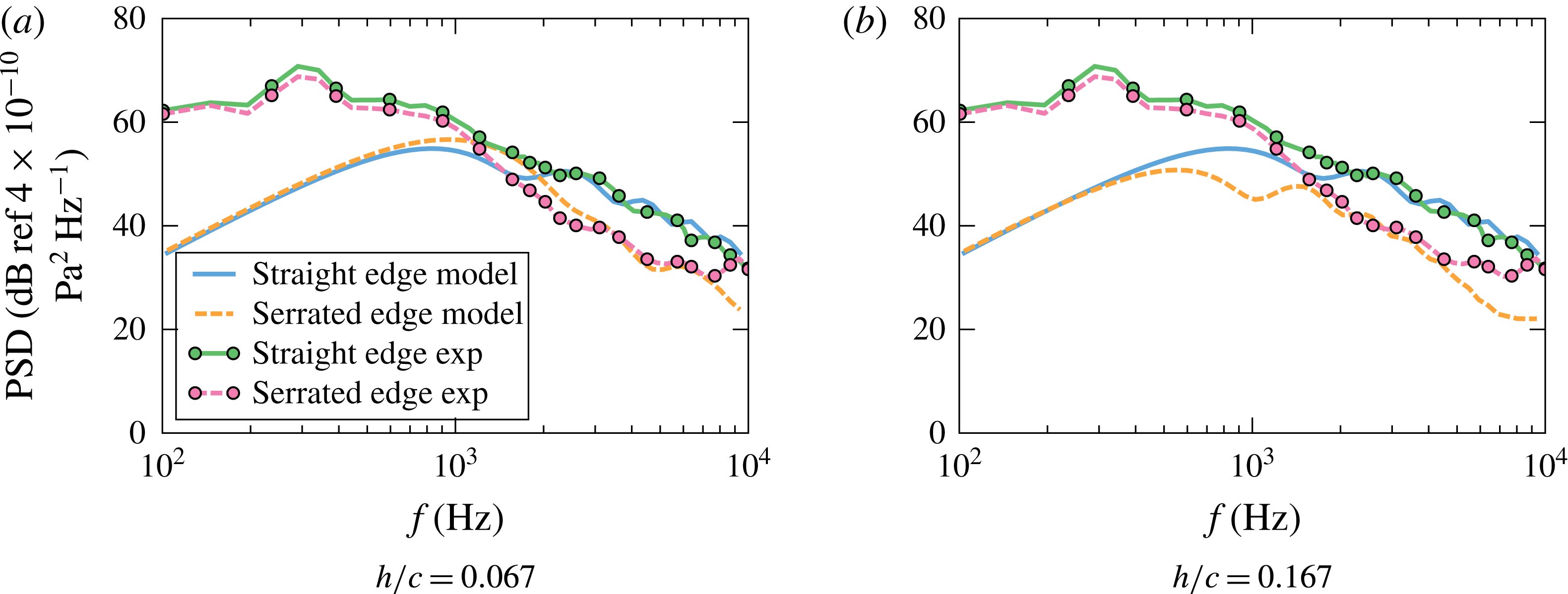
The validation of the second-order model (normalized (2.63) to be consistent with the SPL in the experiment) with experimental data for the baseline (blue) and serrated (red) flat plates. The observer is at
 $90^{\circ }$
above the flat plate in the mid-span plane. The von Kármán model for isotropic turbulence is used with a mean flow velocity of
 $U=60~\text{m}~\text{s}^{-1}$
, integral length scale of
 $L_{t}=0.006~\text{m}$
and turbulence intensity of
 $2.5\,\%$
, as measured by Narayanan et al. (Reference Narayanan, Chaitanya, Haeri, Joseph, Kim and Placsek2015). Both serrations have a spanwise wavelength of
 $\unicode[STIX]{x1D706}/c=0.067$
.

In order to validate the new model, we compare the far-field noise predictions against the experimental data measured by Narayanan et al. (Reference Narayanan, Chaitanya, Haeri, Joseph, Kim and Placsek2015). The experiment was carried out for a flat plate immersed in a turbulent flow with a mean flow velocity of
 $U=60~\text{m}~\text{s}^{-1}$
, turbulence intensity of about
 $2.5\,\%$
and streamwise integral scale of
 $L_{t}=0.006~\text{m}$
. The flat plate had a mean chord length of
 $c\approx 0.175~\text{m}$
and span length of
 $d=0.45~\text{m}$
, fitted with a sinusoidal serration with a spanwise wavelength of
 $\unicode[STIX]{x1D706}/c=0.067$
and amplitudes of
 $h/c=0.067$
(figure 3
a) and
 $h/c=0.167$
(figure 3
b). Note that though in our model a sawtooth serration is used, for such a sharp serration we expect the differences between the two serration profiles to be negligible. Note also that in the experiment the microphones were positioned outside the jet flow in the far-field. However, as pointed out by Amiet (Reference Amiet1975), the shear of the jet mean flow has no refraction effects for the observer directly above the flat plate, i.e.
 $90^{\circ }$
above the flat-plate leading edge. The convection effects of the ambient mean flow, as considered in the model, have an order of
 $\unicode[STIX]{x1D6FD}^{2}$
for such an observer. Since the Mach number in the experiment was low (less than
 $0.2$
), the convection effects of the mean flow can be safely neglected. Therefore, we can proceed to compare the sound spectra measured in the experiment to the results obtained in the model. As mentioned earlier, the von Kármán velocity spectrum, (3.1), was used to represent the energy spectrum of the vertical fluctuation velocity. The high level of noise at low frequencies observed in the experimental data, as mentioned by Narayanan et al. (Reference Narayanan, Chaitanya, Haeri, Joseph, Kim and Placsek2015), is believed to be due to the dominance of the open-jet wind-tunnel background noise and also the grid-generated vortex shedding and its interaction with the flat plate. Therefore, the disagreement at low frequencies between the experiment and model prediction, as shown in figure 3(a), is believed to be due to the dominance of jet noise. Another possible reason for contributing to the disagreement is the perfect-coherence assumption in the streamwise direction, which will be described in detail in § 4.3. In the mid to high frequencies, however, the model provided excellent agreement with measured data. In particular, there exists a perfect match between the predicted and observed peaks of the leading-edge noise of the serrated flat plate at frequencies above
 $f>1000~\text{Hz}$
. This suggests that the model captures the essential physics and gives an accurate prediction of the noise from the flat plates fitted with leading-edge serrations. Predictions under the same flow conditions for a much sharper serration, i.e.
 $\unicode[STIX]{x1D706}/c=0.067$
and
 $h/c=0.167$
, are presented in figure 3(b). It can be seen that sharper serrations are more effective in reducing leading-edge noise, which has been demonstrated by both the experimental data and model predictions. The agreement between the model and experiments continues to be very good in the frequency range where leading-edge noise is dominant. The slight mismatch at high frequencies (
 $f>7~\text{kHz}$
) in the serrated case is likely to be caused by other noise mechanisms present in the experiment, as seen in the experimental data, such as trailing-edge noise.
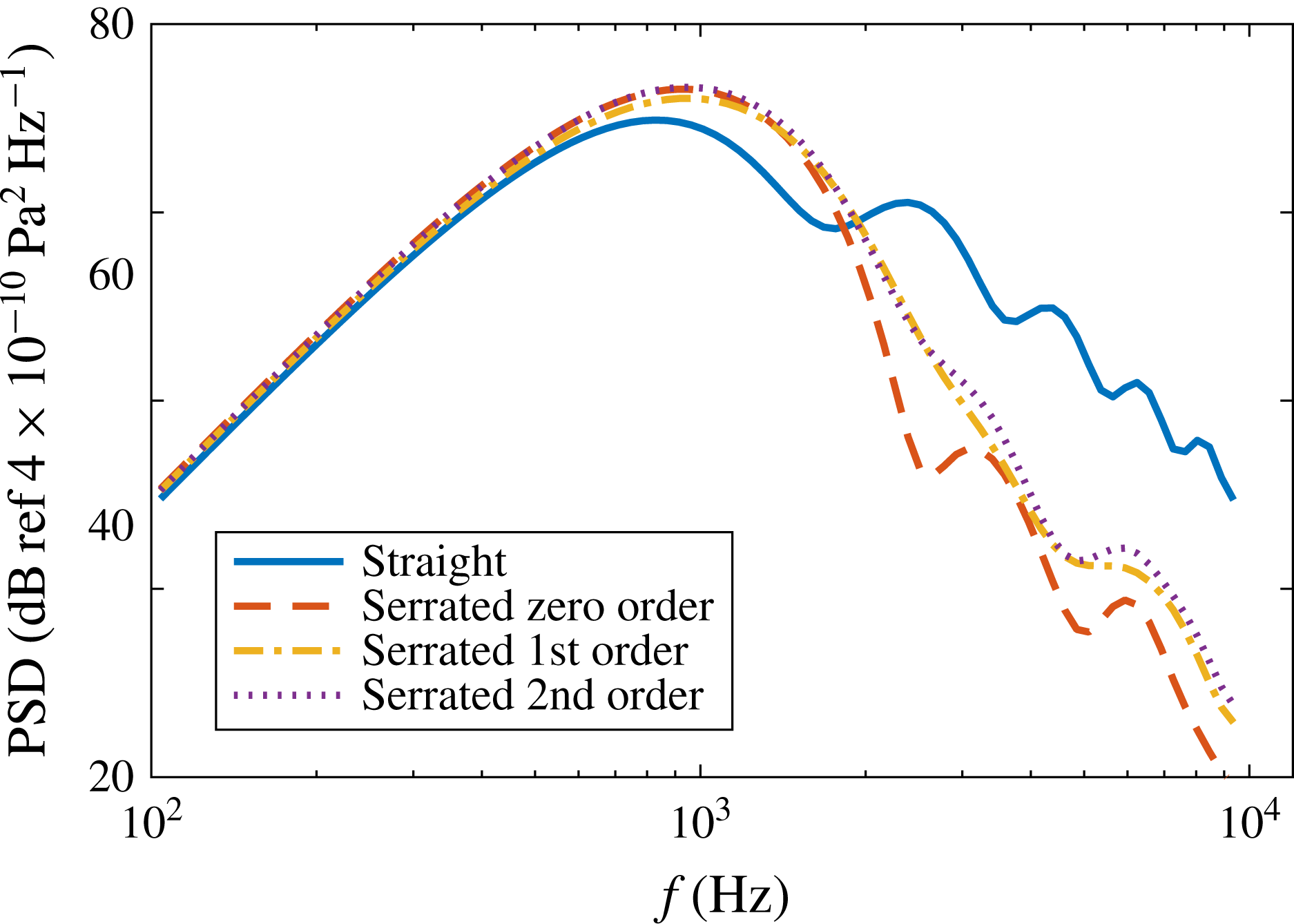
The convergence of the zero-, first- and second-order solutions.

The results presented in figure 3 were calculated using second-order solutions, but we have not yet examined the rate of convergence of the solution in (2.63). To demonstrate that the second-order solution can provide a sufficiently accurate solution, we present the predicted sound pressure spectra for the first validation case (figure 3 a) using the zero-, first- and second-order solutions. The results are shown in figure 4. Though a difference of up to 5 dB can be observed between the zero- and first-order solutions, the difference between the first- and second-order solutions is uniformly less than 1 dB over the entire frequency range of interest. This suggests that the second-order solution should serve as a good approximation for the serration cases considered in this study and over the frequency range of interest.
The effects of varying
 $h$
and
 $\unicode[STIX]{x1D706}$
on a far-field sound spectrum. The observer is located at
 $90^{\circ }$
above the flat plate in the mid-span plane. The von Kármán model for isotropic turbulence is used with the integral length scale of
 $L_{t}=0.006~\text{m}$
and turbulence intensity of
 $2.5\,\%$
, as measured by Narayanan et al. (Reference Narayanan, Chaitanya, Haeri, Joseph, Kim and Placsek2015). The flat plate has a mean chord length of
 $c=0.175~\text{m}$
and a span length of
 $d=0.45~\text{m}$
.

4 Discussions
4.1 Effects of serration geometry
In this section, we carry out a parametric numerical evaluation of the model to study the effects of serration geometry and Mach number on leading-edge noise. Since we are primarily interested in the effects of serration geometry and flow convective effects, we shall use the same chord length and incoming turbulence statistical quantities as in the preceding section, i.e.
 $c\approx 0.175~\text{m}$
,
 $L_{t}=0.006~\text{m}$
and a turbulence intensity of
 $2.5\,\%$
. Results will be presented for the far-field sound power spectra at
 $90^{\circ }$
above the flat plate in the mid-span plane.
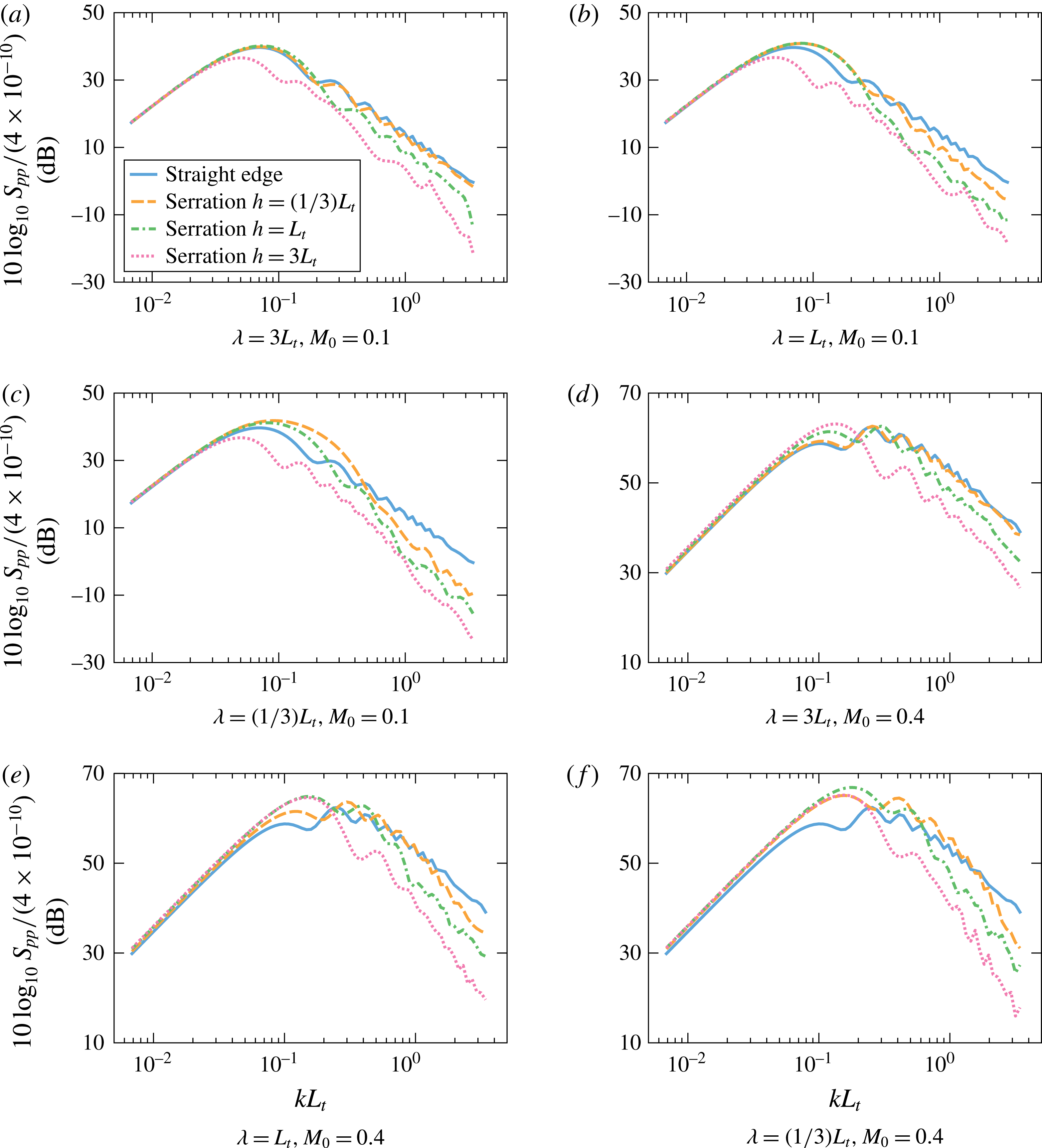
The results in figure 5(a) present the far-field sound pressure level for a flat plate with wide serrations, i.e.
 $\unicode[STIX]{x1D706}=3L_{t}$
, with different amplitudes, i.e.
 $h$
from
 $(1/3)L_{t}$
to
 $3L_{t}$
, in a relatively low Mach number flow of
 $M_{0}=0.1$
. Note here, we use ‘wide’ to describe the serrations which have a longer wavelength
 $\unicode[STIX]{x1D706}$
compared to those to be shown subsequently. Similarly, ‘sharp’ serrations have been used to describe serrations with a small value of
 $\unicode[STIX]{x1D706}$
. It is clear from the results that serrations of
 $h=(1/3)L_{t}$
have virtually no effect on reducing the far-field sound. This is expected since a leading edge with wide and short serrations will act in a similar way to a straight edge. On the other hand, serrations with a relatively large root-to-tip amplitude,
 $h=L_{t}$
, start to reduce noise at high frequencies, as shown by the dash-dotted line in figure 5(a). The use of longer serrations, i.e.
 $h=3L_{t}$
, is shown to result in a significant reduction of far-field noise, even at low frequencies.
Figure 5(b) shows the results for a flat plate with a leading-edge serration wavelength of
 $\unicode[STIX]{x1D706}=L_{t}$
. The effect of varying the serration amplitude (
 $h$
) on the reduction of turbulence interaction noise is similar to that observed before. However, an important difference compared to the wider serration case with
 $\unicode[STIX]{x1D706}=3L_{t}$
, see figure 5(a), is that an area of noise increase appears at low frequencies (around
 $kL_{t}\approx 0.1$
) for short serrations (small
 $h$
). The reason for such noise increases at low frequencies will be discussed later in § 4.3. Results are also presented for very sharp serrations (
 $\unicode[STIX]{x1D706}=(1/3)L_{t}$
), see figure 5(c). The noise increase observed at low frequencies for serrations with small
 $h$
is now more pronounced. However, one can see that as long as the serration is long enough, the noise increase disappears completely and that using sharp serrations (small
 $\unicode[STIX]{x1D706}$
) results in a more effective sound reduction at high frequencies compared with the wide serrations. In summary, the results suggest that in order to suppress leading-edge noise, the serration wavelength
 $\unicode[STIX]{x1D706}$
has to be sufficiently small and the root-to-tip amplitude has to be large.
The effect of flow convective effects, particularly at high Mach numbers, can also be studied using the new model. As mentioned earlier, since the formulations are based on Amiet’s leading-edge noise theory, where the convection effects of the uniform mean flow have been properly accounted for, the new model should suffer no constraints caused by high-speed mean flow convection effects. Therefore the model can be used for higher Mach numbers (when the uniform mean flow assumption is permissible). This capability is particularly important as most of the experimental data available are collected at low Mach numbers of up to
 $0.23$
(Narayanan et al.
Reference Narayanan, Chaitanya, Haeri, Joseph, Kim and Placsek2015). Figure 5(d–f) presents the far-field noise from a flat plate in a turbulent flow with a Mach number of
 $M_{0}=0.4$
. Results are presented for wide (
 $\unicode[STIX]{x1D706}=3L_{t}$
) to sharp (
 $\unicode[STIX]{x1D706}=(1/3)L_{t}$
) serrations. In general, the results show the same trends as before, that is greater noise reduction can be achieved using sharp serrations and that the use of short leading-edge serrations can lead to a noise increase at about
 $kL_{t}=0.1$
. The level of noise increase at low frequencies has been observed to increase significantly with Mach number.
4.2 Directivity
The effects of leading-edge serrations on far-field noise directivity have also been investigated. In this section, we shall study the effects of a specific leading-edge serration on the directivity patterns at different non-dimensionalized frequencies (
 $kL_{t}$
) and Mach numbers (
 $M_{0}=0.1$
and
 $0.4$
). From § 4.1, we see that in order to achieve significant noise reduction, the serration wavelength
 $\unicode[STIX]{x1D706}$
has to be sufficiently small and the serration amplitude
 $2h$
has to be sufficiently large. However, it is found that when
 $\unicode[STIX]{x1D706}$
is too small, e.g.
 $\unicode[STIX]{x1D706}=(1/3)L_{t}$
, there is a large noise increase at low frequencies. Therefore, in practical applications the serration profile with
 $\unicode[STIX]{x1D706}=L_{t}$
and
 $h=3L_{t}$
is preferred. In this section, we choose this geometry to study the effects of serration on directivity at different frequencies and Mach numbers. As before, the flat plate has a mean chord length of
 $c=0.175~\text{m}$
and a span length of
 $d=0.45~\text{m}$
. Also, the incoming flow turbulence intensity is set to
 $2.5\,\%$
and the integral length scale is taken as
 $L_{t}=0.006~\text{m}$
. Results are presented at different acoustic wavenumbers
 $kL_{t}$
, corresponding to the convective wavenumbers of
 $k_{1}L_{t}=0.2,0.5,1,2,5$
and
 $10$
(see figure 6).
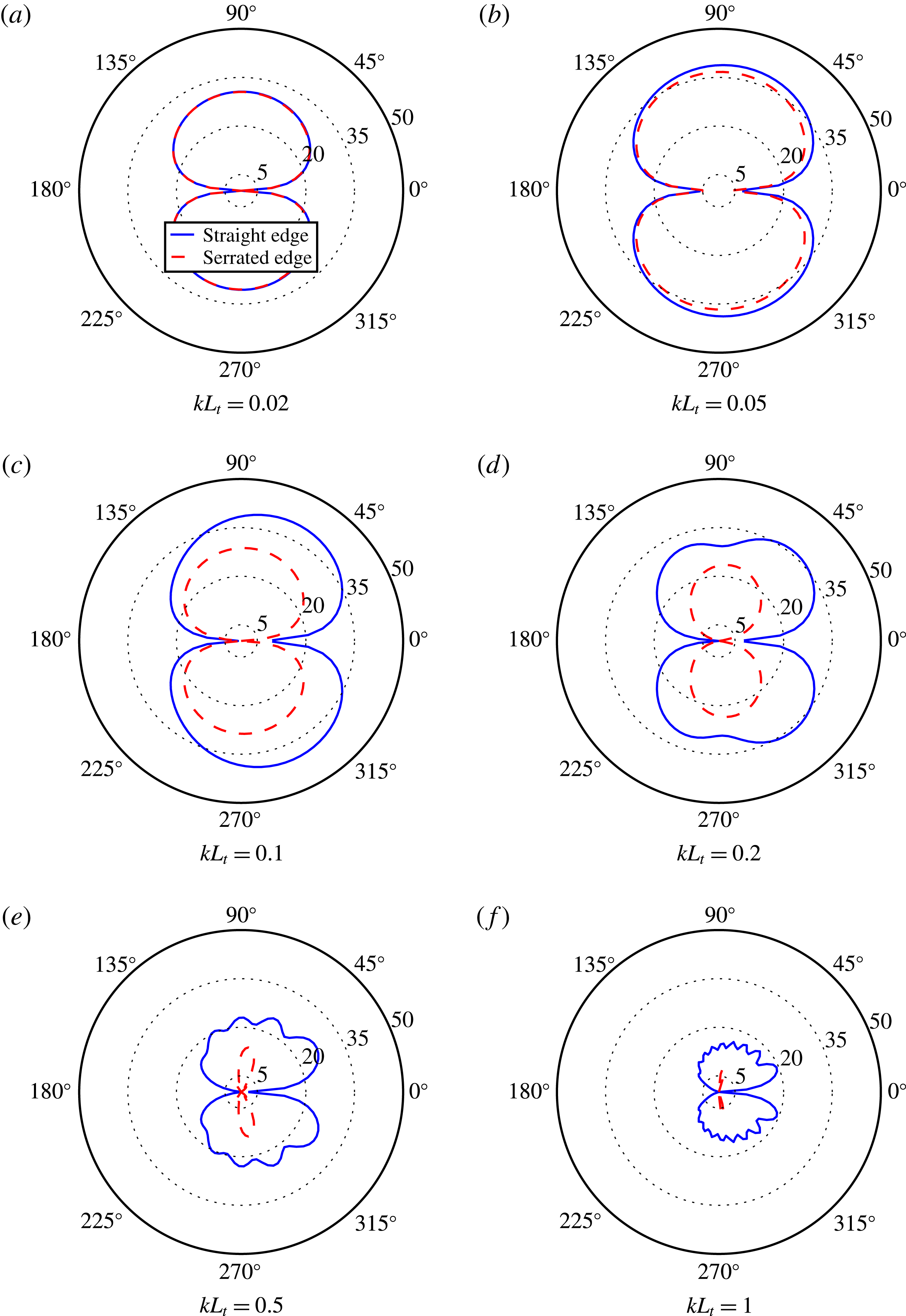
The directivity of leading-edge noise for both straight and serrated edges at Mach number
 $M_{0}=0.1$
in the mid-span plane. The von Kármán model for isotropic turbulence is used in the analytical model with a turbulence intensity of
 $2.5\,\%$
and length scale of
 $L_{t}=0.006~\text{m}$
. Results are presented at different frequencies (
 $kL_{t}$
), corresponding to convective wavenumbers of
 $k_{1}L_{t}=0.2,0.5,1,2,5$
and
 $10$
.

Figure 6(a) shows the directivity patterns for both the straight and serrated edges at a frequency of
 $kL_{t}=0.02$
(
 $k_{1}L_{t}=0.2$
). At such low frequencies, the serrations have no effect on the radiated sound. A slight noise reduction only appears when the frequency increases to
 $kL_{t}=0.05$
(
 $k_{1}L_{t}=0.5$
), as shown in figure 6(b). Further increasing the frequency results in more effective sound reduction, as shown in figure 6(c). It is interesting to note that at mid-frequencies, i.e.
 $kL_{t}=0.2$
and
 $0.5$
(
 $k_{1}L_{t}=2$
and
 $5$
), greater noise reduction is obtained for observer locations closer to the trailing-edge side of the flat plate, i.e.
 $\unicode[STIX]{x1D703}=0^{\circ }$
, see figure 6(d,e). At a higher frequency
 $kL_{t}=1$
(
 $k_{1}L_{t}=10$
), significant noise reduction can be achieved at all radiation angles and the noise reduction at
 $\unicode[STIX]{x1D703}=90^{\circ }$
reaches 10 dB. Another interesting phenomenon observed is the significant change to the directivity pattern of the radiated noise. As seen for the low frequencies, i.e.
 $kL_{t}=0.02$
and
 $0.05$
, the introduction of leading-edge serrations do not significantly change the dipolar shape of the radiated sound field. However, at higher frequencies, the cardioid shape of the leading-edge noise is changed to a more tilted dipolar shape, as seen in figures 6(c) to 6(f). The cause is thought to be due to the fact that for the serrated-edge case the scattered surface pressure is more concentrated near the leading edge and less strong further downstream. From the zero-order solution, equation (2.48), one can see that only the zero mode contributes significantly to the surface pressure far downstream. However, as frequency (
 $k_{1}h$
) increases, this zero mode contribution decreases quickly as
 $|a_{n}|$
decreases. Therefore, for a serrated leading edge, the scattered surface pressure downstream of the leading edge is much less strong than that for the straight edge. This is consistent with the findings in the recent numerical work of Kim et al. (Reference Kim, Haeri and Joseph2016). These more localized dipole sources would produce a nearly dipolar (symmetric) far-field pattern, which explains the significant change in the directivity. The strong scattered pressure far downstream of the straight leading edge is why the pressure integral (2.50) evaluates to large values at small aft angles (small
 $\unicode[STIX]{x1D703}$
), leading to a cardioid directivity pattern. In this sense, by affecting the downstream pressure distribution, the serration contributes to the noise reduction for observers at small aft angles. However, as will be seen in subsequent sections, this is not the primary noise-reduction mechanism. In particular, this would have little impact on the noise at
 $90^{\circ }$
directly above the leading edge. It is also worth noting that the scattered surface pressure is not the only factor that affects the directivity. At high Mach numbers, the convection effects would also become important.
The directivity of leading-edge noise for both straight and serrated edges at Mach number
 $M_{0}=0.4$
in the mid-span plane. The von Kármán model for isotropic turbulence is used in the analytical model with a turbulence intensity of
 $2.5\,\%$
and length scale of
 $L_{t}=0.006~\text{m}$
. Results are presented at different frequencies (
 $kL_{t}$
), corresponding to convective wavenumbers of
 $k_{1}L_{t}=0.2,0.5,1,2,5$
and
 $10$
.

The leading-edge far-field noise OASPL directivity patterns for both straight and serrated leading edges in the mid-span plane. The serration used has a wavelength of
 $\unicode[STIX]{x1D706}=L_{t}$
and a half root-to-tip amplitude of
 $h=3L_{t}$
and the incoming flow has a turbulence intensity of
 $2.5\,\%$
and integral length scale of
 $L_{t}=0.006~\text{m}$
.

The far-field noise directivity results at a Mach number of
 $M_{0}=0.4$
are presented in figure 7. Figure 7(a) shows the directivity results at
 $kL_{t}=0.08$
(
 $k_{1}L_{t}=0.2$
). Compared to figure 6(a) for
 $M_{0}=0.1$
, we see a slight noise increase at low frequencies. This is consistent with our findings in the preceding section, i.e. noise increase is more pronounced at high Mach numbers. This noise increase persists at around
 $90^{\circ }$
above and below the plate for frequencies up to
 $kL_{t}=0.2$
(
 $k_{1}L_{t}=0.5$
), as shown in figure 7(b). The use of leading-edge serrations at
 $kL_{t}=0.4$
(
 $k_{1}L_{t}=1$
), however, leads to noise reduction at all angles, as can be seen in figure 7(c). Figures 7(d) to 7(f) show the directivity patterns at
 $kL_{t}=0.8$
,
 $2$
and
 $4$
, respectively, corresponding to the convective wavenumbers of
 $k_{1}L_{t}=2,5$
and
 $10$
. As before, results here confirm that the leading-edge serrations are more effective at high frequencies and that the use of leading-edge serration changes the far-field noise directivity from a cardioid shape to a tilted dipole.
In addition to the SPL at different frequencies, the overall SPL (OASPL) results can also provide some insight into the total sound energy radiated at different angles and the effects of leading-edge serrations. This also provides an opportunity to better understand the effectiveness of leading-edge serration as most of the OASPL results obtained experimentally are contaminated due to the strong low-frequency background jet noise contribution. The OASPL results, as shown in figure 8, are obtained by integrating the sound power over the frequency range of
 $kL_{t}=0.02$
to
 $2$
(for
 $M_{0}=0.1$
) and
 $kL_{t}=0.04$
to
 $4$
(for
 $M_{0}=0.4$
). As in the previous section, the serration used has a wavelength of
 $\unicode[STIX]{x1D706}=L_{t}$
and a half root-to-tip amplitude of
 $h=3L_{t}$
and the incoming flow has a turbulence intensity of
 $2.5\,\%$
and integral length scale of
 $L_{t}=0.006~\text{m}$
. Results are presented at Mach numbers of
 $M_{0}=0.1$
and
 $0.4$
, see figure 8(a,b). Results have shown that the use of leading-edge serration can result in significant reduction of the OASPL of 5–10 dB. It has also been observed that leading-edge serration is more effective at low Mach numbers and small aft angles. This was also observed in the far-field SPL results in figures 6 and 7 at mid to high frequencies.
4.3 Noise-reduction mechanism
Inspection of the equations developed in § 2 shows that in order for the leading-edge serration treatment to be effective, two geometrical criteria must be met. The detailed derivations are not provided for the sake of brevity, but interested readers can refer to the paper by the authors (Lyu et al.
Reference Lyu, Azarpeyvand and Sinayoko2016b
) on noise from aerofoils with trailing-edge serrations. The two geometrical criteria are (1)
 $\unicode[STIX]{x1D714}h/U\gg 1$
and (2)
 $\unicode[STIX]{x1D714}h_{e}/U\gg 1$
, where the effective half root-to-tip length
 $h_{e}$
is defined by
 $h_{e}=\unicode[STIX]{x1D70E}l_{y^{\prime }}/2$
and
 $l_{y^{\prime }}$
is the spanwise correlation length defined by
 $$\begin{eqnarray}l_{y^{\prime }}(\unicode[STIX]{x1D714})={\displaystyle \frac{1}{R(\unicode[STIX]{x1D714},0)}}\int _{-\infty }^{\infty }R(\unicode[STIX]{x1D714},y^{\prime })\,\text{d}y^{\prime },\end{eqnarray}$$
where
 $R(\unicode[STIX]{x1D714},y^{\prime })$
is the spanwise two-point correlation of the incoming turbulent velocity. Using the von Kármán model, Amiet (Reference Amiet1975) showed that
 $l_{y^{\prime }}(\unicode[STIX]{x1D714})$
can be obtained as
 $$\begin{eqnarray}l_{y^{\prime }}(\unicode[STIX]{x1D714})={\displaystyle \frac{16L_{t}}{3}}\left({\displaystyle \frac{\unicode[STIX]{x1D6E4}(1/3)}{\unicode[STIX]{x1D6E4}(5/6)}}\right)^{2}{\displaystyle \frac{(\unicode[STIX]{x1D714}/Uk_{e})^{2}}{\left(3+8(\unicode[STIX]{x1D714}/Uk_{e})^{2}\right)\sqrt{1+(\unicode[STIX]{x1D714}/Uk_{e})^{2}}}}.\end{eqnarray}$$
It may seem somewhat unexpected to obtain the dependence of the sound reduction on the spanwise correlation length. A careful inspection of (2.59) reveals that this dependence originates from the energy spectrum
 $\unicode[STIX]{x1D6F7}_{ww}(\unicode[STIX]{x1D714},k_{2})$
in (2.59). The inverse Fourier transformation of
 $\unicode[STIX]{x1D6F7}_{ww}(\unicode[STIX]{x1D714},k_{2})$
over
 $k_{2}$
yields the two-point cross spectrum
 $R(\unicode[STIX]{x1D714},y^{\prime })$
. The first criterion is consistent with the findings in the numerical work by Lau et al. (Reference Lau, Haeri and Kim2013) and some experimental data available for different leading-edge serrations (Chaitanya et al.
Reference Chaitanya, Narayanan, Joseph and Kim2016). The second criterion, although less discussed in recent work, is an important condition and relates the serration geometry to the structure of the incoming turbulence.
As shown in other numerical and experimental work, the main cause of noise reduction is the destructive sound interferences caused by the serration. In that sense, the noise-reduction mechanism is very similar to that of trailing-edge serration, as previously discussed by Lyu et al. (Reference Lyu, Azarpeyvand and Sinayoko2016b
). A better understanding of the destructive sound interference phenomenon may help us to explain the physical implications of the two above-mentioned criteria. The first condition
 $\unicode[STIX]{x1D714}h/U\gg 1$
is to ensure that a complete phase variation (of minimum
 $2\unicode[STIX]{x03C0}$
) of the scattered pressure along the serrated edge is achieved. At low frequencies, this requires the serration amplitude
 $2h$
to be large in order to achieve significant sound reduction, as only a large value of
 $h$
can ensure a complete phase variation of the scattered pressure field along the serrated edge. For cases where the serration amplitude
 $h$
is not large enough, there would be little variation in the scattered pressure, i.e. in-phase radiation along the edge. This can result in noise increase at low frequencies, as observed in figures 3 and 5, which is due to the fact that the wetted edge by an in-phase pressure field for the serrated edge is longer than that of the straight-edge. It should be noted that in this paper we assume that the incoming turbulence is frozen. This would imply a perfect spatial correlation in the streamwise direction for the upwash velocity field. For serrations with a large
 $h$
, the assumption of perfect streamwise correlation of the turbulence becomes inappropriate and therefore the condition developed may not hold. This might explain why a noise increase is predicted in figure 3(a) while this was not seen in the experimental results. However, for mid- to high-frequency regimes this assumption should serve as a good approximation, as demonstrated by figure 3(a,b). The importance of the second criterion is also easy to understand. Since noise reduction relies on destructive interference, the scattered pressure needs to be correlated. In this case
 $\unicode[STIX]{x1D714}h_{e}/U\gg 1$
effectively ensures this, hence makes pressure cancellation due to phase variation possible.
The effects of varying
 $\unicode[STIX]{x1D714}h/U$
on the scattered surface pressure at a fixed frequency and
 $\unicode[STIX]{x1D714}h_{e}/U=7$
: (a)
 $\unicode[STIX]{x1D714}h/U=1$
; (b)
 $\unicode[STIX]{x1D714}h/U=4$
; (c)
 $\unicode[STIX]{x1D714}h/U=10$
; (d)
 $\unicode[STIX]{x1D714}h/U=20$
. The colour shows the normalized scattered pressure on the upper surface of the flat plate. The vertical axis shows the spanwise coordinate normalized by the spanwise correlation length and the horizontal axis shows the streamwise coordinate normalized by the hydrodynamic wavelength.

The effects of varying
 $\unicode[STIX]{x1D714}h_{e}/U$
on the scattered surface pressure at a fixed frequency and
 $\unicode[STIX]{x1D714}h/U=10$
: (a)
 $\unicode[STIX]{x1D714}h_{e}/U=1$
; (b)
 $\unicode[STIX]{x1D714}h_{e}/U=3$
; (c)
 $\unicode[STIX]{x1D714}h_{e}/U=6$
; (d)
 $\unicode[STIX]{x1D714}h_{e}/U=10$
. The colour shows the normalized scattered pressure on the upper surface of the flat plate. The vertical axis shows the spanwise coordinate normalized by the spanwise correlation length and the horizontal axis shows the streamwise coordinate normalized by the hydrodynamic wavelength.

To clearly demonstrate the effect of the
 $\unicode[STIX]{x1D714}h/U$
criterion, we present the scattered pressure on the upper surface of the flat plate at fixed
 $\unicode[STIX]{x1D714}h_{e}/U=7$
in figure 9. To better understand the effect of sound interference, the
 $x^{\prime }$
- and
 $y^{\prime }$
-axis are normalized by the hydrodynamic wavelength (
 $\unicode[STIX]{x1D706}_{h}=2\unicode[STIX]{x03C0}U/\unicode[STIX]{x1D714}$
) and spanwise correlation length (
 $l_{y^{\prime }}$
). The distances between the adjacent
 $y^{\prime }$
-grid lines shown in figure 9 are used to show the spanwise correlation length
 $l_{y^{\prime }}$
. When
 $\unicode[STIX]{x1D714}h/U=1$
, as can be seen from figure 9(a), little phase variation is induced along and near the leading edge in the spanwise direction. This suggests little sound reduction occurs due to destructive interference. As
 $\unicode[STIX]{x1D714}h/U$
increases to
 $4$
, as shown in figure 9(b), phase variation of the scattered pressure near the leading edge become noticeable. Further increasing
 $\unicode[STIX]{x1D714}h/U$
to
 $10$
, we see from figure 9(c) that significant sound reduction can be achieved due to the strong phase variation near the leading edge in the spanwise direction. Figure 9(d) shows that pressure distribution when
 $\unicode[STIX]{x1D714}h/U=20$
. It is evident that when
 $\unicode[STIX]{x1D714}h_{e}/U$
is fixed, the number of pressure crests and troughs within
 $l_{y^{\prime }}$
is fixed at sufficiently large values of
 $\unicode[STIX]{x1D714}h/U$
(see figure 9
b–d). The effects of
 $\unicode[STIX]{x1D714}h_{e}/U$
are similarly shown in figure 10, where
 $\unicode[STIX]{x1D714}h/U$
is fixed at
 $10$
while
 $\unicode[STIX]{x1D714}h_{e}/U$
varies from
 $1$
to
 $10$
. From figure 10(a–d) the scattered pressure patterns are virtually the same. However, the phase variation of the surface pressure within the spanwise correlation length
 $l_{y^{\prime }}$
is very different. In figure 10(a) we see that within the length of
 $l_{y^{\prime }}$
(between adjacent
 $y^{\prime }$
-grid lines), the phase variation of pressure is negligible. Since destructive interference can only occur within
 $l_{y^{\prime }}$
, little sound reduction can be expected in this case. On the other hand, figure 10(c,d) shows a sufficient number of crests and troughs appearing within the length
 $l_{y^{\prime }}$
, leading to effective noise reduction due to the destructive interference within
 $l_{y^{\prime }}$
. Figures 9 and 10 clearly show that in order to achieve significant sound reduction both
 $\unicode[STIX]{x1D714}h/U\gg 1$
and
 $\unicode[STIX]{x1D714}h_{e}/U\gg 1$
have to be satisfied.
5 Conclusions and future work
A new mathematical model is developed in this paper with the aim of predicting the sound radiated from the interaction of an incoming turbulent flow with a flat plate with a serrated leading edge. By making use of Fourier expansion and Schwarzschild techniques, we find that the PSD of the far-field sound is related to the energy spectrum of the incident velocity field. The model is based on Amiet’s approach and is therefore valid even for high Mach number applications where leading-edge noise is a common problem. Comparing the model with experimental data has shown excellent agreement and this suggests that the model can capture the essential physics of the noise-generation and reduction mechanisms and can provide an accurate prediction of the noise from serrated leading edges. A thorough parametric study has been carried out using the new model and the effects of leading-edge serration geometry and incoming turbulent flow characteristics on far-field noise at different Mach numbers have been studied. It has been found that in order to achieve significant noise reduction, the serration amplitude
 $2h$
has to be sufficiently large compared to the hydrodynamic wavelength in the streamwise direction. More specifically, the condition of
 $\unicode[STIX]{x1D714}h/U\gg 1$
needs to be satisfied. The spanwise correlation length also plays an important role in achieving effective noise reduction. In order to achieve significant noise reduction, a second condition of
 $\unicode[STIX]{x1D714}h_{e}/U\gg 1$
has to be satisfied, which ensures that scattered pressure is correlated for a possible destructive interference to occur. It has also been shown that leading-edge serration can effectively reduce the far-field noise at even high Mach numbers. However, larger serrations might be needed especially in the relatively low frequency regimes. From the far-field noise directivity patterns, it has been observed that more sound reduction occurs at small aft angles and the noise directivity at high frequencies changes from a cardioid shape to a tilted dipole-like pattern. The mathematical model developed in this paper has shown that destructive sound interference is the primary noise-reduction mechanism, especially in the mid- to high-frequency regime where leading-edge noise is most effectively reduced using serrations. Further work is needed to address the issue of perfect coherence for the incoming turbulence in the streamwise direction, which might not be an accurate assumption at low frequencies.
Acknowledgements
The first author (B.L.) gratefully acknowledges the financial support provided by the Cambridge Commonwealth European and International Trust and China Scholarship Council. The second author (M.A.) would like to acknowledge the financial support of the Royal Academy of Engineering.
Appendix A
A.1 Second iterated results
The zero- and first-order solutions of
 $\unicode[STIX]{x1D6F7}_{t}(x,0)$
are given by (2.42) and 2.43, respectively, in § 2. The second-order solution is given by
 $C_{n^{\prime }}^{(2)}(x)$
as follows:
 $$\begin{eqnarray}\displaystyle C_{n^{\prime }}^{(2)}(x) & = & \displaystyle -\unicode[STIX]{x1D6F7}_{ia}(1+\text{i})\text{e}^{\text{i}k_{1}x}\mathop{\sum }_{m=-\infty }^{\infty }\Bigg\{\unicode[STIX]{x1D6FD}_{n^{\prime }m}(\text{i}k_{1})^{2}(E^{\ast }(\unicode[STIX]{x1D707}_{n^{\prime }}x)-E^{\ast }(\unicode[STIX]{x1D707}_{m}x))\nonumber\\ \displaystyle & & \displaystyle +\,(\unicode[STIX]{x1D6FD}_{n^{\prime }m}\text{i}k_{1}+\unicode[STIX]{x1D6FE}_{n^{\prime }m}\text{i}(k_{1}-\unicode[STIX]{x1D707}_{m}))\sqrt{{\displaystyle \frac{\unicode[STIX]{x1D707}_{m}}{2\unicode[STIX]{x03C0}x}}}(\text{e}^{-\text{i}\unicode[STIX]{x1D707}_{n^{\prime }}x}-\text{e}^{-\text{i}\unicode[STIX]{x1D707}_{m}x})\nonumber\\ \displaystyle & & \displaystyle -\,{\displaystyle \frac{\unicode[STIX]{x1D6FE}_{n^{\prime }m}}{2}}\left(\sqrt{{\displaystyle \frac{\unicode[STIX]{x1D707}_{m}}{2\unicode[STIX]{x03C0}x}}}{\displaystyle \frac{1}{x}}(\text{e}^{-\text{i}\unicode[STIX]{x1D707}_{n^{\prime }}x}-\text{e}^{-\text{i}\unicode[STIX]{x1D707}_{m}x})+\text{i}(\unicode[STIX]{x1D707}_{n^{\prime }}-\unicode[STIX]{x1D707}_{m})\sqrt{{\displaystyle \frac{\unicode[STIX]{x1D707}_{m}}{2\unicode[STIX]{x03C0}x}}}\text{e}^{-\text{i}\unicode[STIX]{x1D707}_{n^{\prime }}x}\right)\Bigg\},\qquad\end{eqnarray}$$
where
 $$\begin{eqnarray}\displaystyle & \displaystyle \unicode[STIX]{x1D6FD}_{ln}=\mathop{\sum }_{m=-\infty }^{\infty }(\unicode[STIX]{x1D6FC}_{ln}a_{m}-(B_{lm}/(k_{2l}^{2}-k_{2n}^{2}))a_{n})\unicode[STIX]{x1D6FC}_{nm}, & \displaystyle\end{eqnarray}$$
 $$\begin{eqnarray}\displaystyle & \displaystyle \unicode[STIX]{x1D6FE}_{ln}=\mathop{\sum }_{m=-\infty }^{\infty }(\unicode[STIX]{x1D6FC}_{ln}a_{m}\sqrt{\unicode[STIX]{x1D707}_{m}/\unicode[STIX]{x1D707}_{n}}-(B_{lm}/(k_{2l}^{2}-k_{2n}^{2}))a_{n})\unicode[STIX]{x1D6FC}_{nm}. & \displaystyle\end{eqnarray}$$
Similarly,
 $P_{n^{\prime }}^{(2)}(x)$
can be expressed as
 $$\begin{eqnarray}\displaystyle P_{n^{\prime }}^{(2)}(x) & = & \displaystyle \unicode[STIX]{x1D70C}_{0}U\unicode[STIX]{x1D6F7}_{ia}(1+\text{i})\text{e}^{\text{i}k_{1}x}\nonumber\\ \displaystyle & & \displaystyle \mathop{\sum }_{m=-\infty }^{\infty }\Bigg\{\unicode[STIX]{x1D6FD}_{n^{\prime }m}(\text{i}k_{1})^{2}{\displaystyle \frac{1}{\sqrt{2\unicode[STIX]{x03C0}x}}}(\sqrt{\unicode[STIX]{x1D707}_{n^{\prime }}}\text{e}^{-\text{i}\unicode[STIX]{x1D707}_{n^{\prime }}x}-\sqrt{\unicode[STIX]{x1D707}_{m}}\text{e}^{-\text{i}\unicode[STIX]{x1D707}_{m}x})\nonumber\\ \displaystyle & & \displaystyle -\,(\unicode[STIX]{x1D6FD}_{n^{\prime }m}\text{i}k_{1}+\unicode[STIX]{x1D6FE}_{n^{\prime }m}\text{i}(k_{1}-\unicode[STIX]{x1D707}_{m}))\bigg[\text{i}\sqrt{{\displaystyle \frac{\unicode[STIX]{x1D707}_{m}}{2\unicode[STIX]{x03C0}x}}}(\unicode[STIX]{x1D707}_{n^{\prime }}\text{e}^{-\text{i}\unicode[STIX]{x1D707}_{n^{\prime }}x}-\unicode[STIX]{x1D707}_{m}\text{e}^{-\text{i}\unicode[STIX]{x1D707}_{m}x})\nonumber\\ \displaystyle & & \displaystyle +\,{\displaystyle \frac{1}{2}}\sqrt{{\displaystyle \frac{\unicode[STIX]{x1D707}_{m}}{2\unicode[STIX]{x03C0}x}}}{\displaystyle \frac{1}{x}}(\text{e}^{-\text{i}\unicode[STIX]{x1D707}_{n^{\prime }}x}-\text{e}^{-\text{i}\unicode[STIX]{x1D707}_{m}x})\bigg]\nonumber\\ \displaystyle & & \displaystyle +\,\unicode[STIX]{x1D6FE}_{n^{\prime }m}\bigg[\text{i}{\displaystyle \frac{1}{2}}\sqrt{{\displaystyle \frac{\unicode[STIX]{x1D707}_{m}}{2\unicode[STIX]{x03C0}x}}}{\displaystyle \frac{1}{x}}(\unicode[STIX]{x1D707}_{n^{\prime }}\text{e}^{-\text{i}\unicode[STIX]{x1D707}_{n^{\prime }}x}-\unicode[STIX]{x1D707}_{m}\text{e}^{-\text{i}\unicode[STIX]{x1D707}_{m}x})\nonumber\\ \displaystyle & & \displaystyle +\,{\displaystyle \frac{1}{2}}{\displaystyle \frac{3}{2}}\sqrt{{\displaystyle \frac{\unicode[STIX]{x1D707}_{m}}{2\unicode[STIX]{x03C0}x}}}{\displaystyle \frac{1}{x^{2}}}(\text{e}^{-\text{i}\unicode[STIX]{x1D707}_{n^{\prime }}x}-\text{e}^{-\text{i}\unicode[STIX]{x1D707}_{m}x})\nonumber\\ \displaystyle & & \displaystyle +\,\text{i}{\displaystyle \frac{(\unicode[STIX]{x1D707}_{n^{\prime }}-\unicode[STIX]{x1D707}_{m})}{2}}(\text{i}\unicode[STIX]{x1D707}_{n^{\prime }}\sqrt{{\displaystyle \frac{\unicode[STIX]{x1D707}_{m}}{2\unicode[STIX]{x03C0}x}}}\text{e}^{-\text{i}\unicode[STIX]{x1D707}_{n^{\prime }}x}+{\displaystyle \frac{1}{2}}\sqrt{{\displaystyle \frac{\unicode[STIX]{x1D707}_{m}}{2\unicode[STIX]{x03C0}x}}}{\displaystyle \frac{1}{x}}\text{e}^{-\text{i}\unicode[STIX]{x1D707}_{n^{\prime }}x})\bigg]\Bigg\}.\end{eqnarray}$$
Finally,
 $\unicode[STIX]{x1D6E9}_{n^{\prime }}^{(2)}$
can be found as
 $$\begin{eqnarray}\displaystyle \unicode[STIX]{x1D6E9}_{n^{\prime }}^{(2)} & = & \displaystyle \mathop{\sum }_{m=-\infty }^{\infty }\Bigg\{\unicode[STIX]{x1D6FD}_{n^{\prime }m}(\text{i}k_{1})^{2}(\sqrt{\unicode[STIX]{x1D707}_{n^{\prime }}}S_{n^{\prime }n^{\prime }}-\sqrt{\unicode[STIX]{x1D707}_{m}}S_{n^{\prime }m})\nonumber\\ \displaystyle & & \displaystyle -\,(\unicode[STIX]{x1D6FD}_{n^{\prime }m}\text{i}k_{1}+\unicode[STIX]{x1D6FE}_{n^{\prime }m}\text{i}(k_{1}-\unicode[STIX]{x1D707}_{m}))[\text{i}\sqrt{\unicode[STIX]{x1D707}_{m}}(\unicode[STIX]{x1D707}_{n^{\prime }}S_{n^{\prime }n^{\prime }}-\unicode[STIX]{x1D707}_{m}S_{n^{\prime }m})+\sqrt{\unicode[STIX]{x1D707}_{m}}(T_{n^{\prime }n^{\prime }}-T_{n^{\prime }m})]\nonumber\\ \displaystyle & & \displaystyle +\,\unicode[STIX]{x1D6FE}_{n^{\prime }m}\bigg[\text{i}\sqrt{\unicode[STIX]{x1D707}_{m}}(\unicode[STIX]{x1D707}_{n^{\prime }}T_{n^{\prime }n^{\prime }}-\unicode[STIX]{x1D707}_{m}T_{n^{\prime }m})+\sqrt{\unicode[STIX]{x1D707}_{m}}(V_{n^{\prime }n^{\prime }}-V_{n^{\prime }m})\nonumber\\ \displaystyle & & \displaystyle +\,\text{i}{\displaystyle \frac{(\unicode[STIX]{x1D707}_{n^{\prime }}-\unicode[STIX]{x1D707}_{m})}{2}}(\text{i}\unicode[STIX]{x1D707}_{n^{\prime }}\sqrt{\unicode[STIX]{x1D707}_{m}}S_{n^{\prime }n^{\prime }}+\sqrt{\unicode[STIX]{x1D707}_{m}}T_{n^{\prime }n^{\prime }})\bigg]\Bigg\},\end{eqnarray}$$
where function
 $V_{nm}$
is given by
 $$\begin{eqnarray}\displaystyle V_{nm} & = & \displaystyle \mathop{\sum }_{j=0}^{1}\Bigg\{{\displaystyle \frac{1}{\unicode[STIX]{x1D70E}_{j}}}\text{e}^{\text{i}\unicode[STIX]{x1D705}_{ij}(\unicode[STIX]{x1D706}_{j}+(c-\unicode[STIX]{x1D716}_{j})/\unicode[STIX]{x1D70E}_{j})}\nonumber\\ \displaystyle & & \displaystyle \times \bigg[{\displaystyle \frac{1}{\sqrt{2\unicode[STIX]{x03C0}(c-\unicode[STIX]{x1D716}_{j})}}}\text{e}^{-\text{i}\unicode[STIX]{x1D702}_{Bnmj}(c-\unicode[STIX]{x1D716}_{j})}-{\displaystyle \frac{1}{\sqrt{2\unicode[STIX]{x03C0}(c-\unicode[STIX]{x1D716}_{j+1})}}}\text{e}^{-\text{i}\unicode[STIX]{x1D702}_{Bnmj}(c-\unicode[STIX]{x1D716}_{j+1})}\bigg]\nonumber\\ \displaystyle & & \displaystyle +\,{\displaystyle \frac{1}{\text{i}\unicode[STIX]{x1D705}_{nj}}}\Bigg({\displaystyle \frac{-\text{i}\unicode[STIX]{x1D702}_{Am}}{\sqrt{\unicode[STIX]{x1D702}_{Am}}}}[\text{e}^{\text{i}\unicode[STIX]{x1D705}_{nj}\unicode[STIX]{x1D706}_{j+1}}E^{\ast }(\unicode[STIX]{x1D702}_{Am}(c-\unicode[STIX]{x1D716}_{j+1}))-\text{e}^{\text{i}\unicode[STIX]{x1D705}_{nj}\unicode[STIX]{x1D706}_{j}}E^{\ast }(\unicode[STIX]{x1D702}_{Am}(c-\unicode[STIX]{x1D716}_{j}))]\nonumber\\ \displaystyle & & \displaystyle +\,{\displaystyle \frac{\text{i}\unicode[STIX]{x1D702}_{Bnmj}}{\sqrt{\unicode[STIX]{x1D702}_{Bnmj}}}}\text{e}^{\text{i}\unicode[STIX]{x1D705}_{nj}(\unicode[STIX]{x1D706}_{j}+(c-\unicode[STIX]{x1D716}_{j})/\unicode[STIX]{x1D70E}_{j})}\nonumber\\ \displaystyle & & \displaystyle \times \,[E^{\ast }(\unicode[STIX]{x1D702}_{Bnmj}(c-\unicode[STIX]{x1D716}_{j+1}))-E^{\ast }(\unicode[STIX]{x1D702}_{Bnmj}(c-\unicode[STIX]{x1D716}_{j}))]\Bigg)\Bigg\}.\end{eqnarray}$$