


INTRODUCTION
Predictions of substantial global population increases, challenges in adapting to climate change, as well as anticipated changes in diets and consumption patterns by 2050, have raised concerns about food security in the decades ahead (Tilman et al. Reference Tilman, Balzer, Hill and Befort2011; Ray et al. Reference Ray, Mueller, West and Foley2013; Fischer et al. Reference Fischer, Byerlee and Edmeades2014; Keating et al. Reference Keating, Herrero, Carberry, Gardner and Cole2014). This concern arises against a backdrop of crop yield plateaus and reductions in rates of yield increase observed in recent years, despite technological improvements (Ray et al. Reference Ray, Ramankutty, Mueller, West and Foley2012; Grassini et al. Reference Grassini, Eskridge and Cassman2013). Keating et al. (Reference Keating, Herrero, Carberry, Gardner and Cole2014) identified 14 pathways to meeting expected food demand, of which an important component is closing yield gaps in existing crop and livestock production systems. Wheat yields globally range from 40–95% of yield potentials, estimated using model simulations (Lobell et al. Reference Lobell, Cassman and Field2009), or 61–80% of potential yields, derived primarily from crop variety trials (Fischer et al. Reference Fischer, Byerlee and Edmeades2014), so large production gains on existing cropping land should be feasible in areas where yield gaps are large. Although Australian wheat yields are relatively low compared with high-yielding regions such as China and Northern Europe, Australia is an important wheat supplier in global markets and accounts for 0·12 of global wheat exports (ABARES 2012), which is a significant buffer to annual regional shortages around the globe. To most effectively address yield gaps in Australian wheat cropping systems, and thus contribute to global food security, requires an improved understanding of how Australian wheat production is performing, in order to direct efforts to increase production sustainably by reducing yield gaps.
In rainfed cropping systems, the yield gap (Yg) is defined as the difference between average actual yields (Ya) currently achieved by farmers and the benchmark water-limited yield (Yw). Water-limited yield is the yield which could be achieved under best-practice management, in the absence of nutrient limitations, pests and diseases, but subject to environmental constraints such as temperature, solar radiation and rainfall (van Ittersum et al. Reference van Ittersum, Cassman, Grassini, Wolf, Tittonell and Hochman2013). Relative yield (Y%) is the ratio of Ya to Yw expressed as a percentage and is a useful indicator of production as a function of potential. A Y% of 80% is regarded as the upper range of wheat yields consistently achieved by leading farmers over a number of seasons in Australia (van Rees et al. Reference van Rees, McClelland, Hochman, Carberry, Hunt, Huth and Holzworth2014) and for rainfed crops globally (Lobell et al. Reference Lobell, Cassman and Field2009). The exploitable yield represents additional yield that would be harvested if 80% of Yw is achieved (Exploitable yield = ((Yw × 0·8) − Ya)), with economic and climatic uncertainties constraining yields to within this range (Lobell et al. Reference Lobell, Cassman and Field2009).
Within Australia, studies have reported comparable yield gaps using varying methods and at a range of scales. At a sub-farm scale, Oliver & Robertson (Reference Oliver and Robertson2013) showed Y% below 50% on 0·31 of one farm, between 50 and 75% on 0·53 of the farm and higher than 75% on 0·15 of the farm. At a regional scale, Hochman et al. (Reference Hochman, Gobbett, Holzworth, McClelland, van Rees, Marinoni, Navarro Garcia and Horan2012) reported a mean of 53% for the Wimmera region of Southeastern Australia (an area of 435 000 ha) over 20 years. Estimated farm yields and potential yields over the Western Australia wheat belt show a Y% of 69% in 2010 (Fischer et al. Reference Fischer, Byerlee and Edmeades2014). Insights into the upper range of achievable yield have been obtained through studies of yields obtained by leading farmers who employ agronomic consultants, have been early technology adopters, use decision support tools and best management cropping practices, and have retained detailed soil testing and rainfall records. The highest Y% reported for Australian wheat farms include a study of leading growers nationally (2004–08) with Y% of 77% (Hochman et al. Reference Hochman, Holzworth and Hunt2009), and a study of three leading farmers over 16–20 years showed Y% of 74–82% (van Rees et al. Reference van Rees, McClelland, Hochman, Carberry, Hunt, Huth and Holzworth2014). Although the different spatial scales, farmer sub-sets and methodologies used in the above studies make formal comparisons among them difficult, the results provide clear indications that there is scope for many farmers to increase yields on existing farmlands.
The case for a global estimate of yield gaps based on locally relevant and credible assessment of the yield gaps of the world's major crops was made by van Ittersum et al. (Reference van Ittersum, Cassman, Grassini, Wolf, Tittonell and Hochman2013), who outlined the case and methodology for developing the Global Yield Gap Atlas (GYGA). This methodology, herein referred to as the ‘GYGA protocol’, is outlined by Van Wart et al. (Reference Van Wart, van Bussel, Wolf, Licker, Grassini, Nelson, Boogaard, Gerber, Mueller, Claessens, van Ittersum and Cassman2013b ), van Bussel et al. (Reference van Bussel, Grassini, Van Wart, Wolf, Claessens, Yang, Boogaard, de Groot, Saito, Cassman and van Ittersum2015) and Grassini et al. (Reference Grassini, van Bussel, Van Wart, Wolf, Claessens, Yang, Boogaard, de Groot, van Ittersum and Cassman2015), can be applied to major cropping systems in both data-rich and data-poor contexts, and facilitates comparisons among countries, or between regions within the same country. The protocol includes methods to upscale yield and yield gap estimates from reference weather stations to climate zones and national level (van Bussel et al. Reference van Bussel, Grassini, Van Wart, Wolf, Claessens, Yang, Boogaard, de Groot, Saito, Cassman and van Ittersum2015) by using a targeted climate zoning system (Van Wart et al. Reference Van Wart, van Bussel, Wolf, Licker, Grassini, Nelson, Boogaard, Gerber, Mueller, Claessens, van Ittersum and Cassman2013b ). Tiered data selection methodologies (Grassini et al. Reference Grassini, van Bussel, Van Wart, Wolf, Claessens, Yang, Boogaard, de Groot, van Ittersum and Cassman2015) ensure that the highest quality data and locally relevant expertise is used first, but where necessary, progressively lower-quality data may be incorporated into the analysis. Readers are referred to these publications for a more detailed description and justification of these protocols.
The Australian wheat crop is a challenging case study for implementing the GYGA protocol because it extends over a large area with diverse and variable climatic and soil conditions. On the positive side, it has mostly homogenous topography and is relatively data-rich. The current study represents a first attempt at applying this consistent protocol to derive estimates of the yield gap of rainfed wheat in Australia. The use of a globally applicable protocol enables the comparison of wheat Yg in Australia with other parts of the world. To demonstrate the opportunities that arise from a global protocol, the data generated from applying the GYGA methodology were used to explore relationships among factors contributing to the yield gap.
MATERIALS AND METHODS
Study area and cropping system
Wheat cropping areas in Australia mainly (0·87) receive between 300 and 600 mm rainfall annually, with 0·46 of areas receiving 300–400 mm, 0·24 receiving 400–500 mm and 0·17 receiving 500–600 mm (figures derived using GIS analysis summarizing area of cereals (ABARE-BRS 2010) occurring within zones of mean annual rainfall (1961–90, BoM 2009). National agricultural survey data over the period 1996–2010 report that the average size of ‘wheat and other cropping’ farms was 2003 ha, of which an average 0·50 was cropped. Of the cropped area, 0·56 was planted to wheat (ABARES 2015). A survey of Australian grain producers (Edwards et al. Reference Edwards, Umbers and Wentworth2012) found that wheat comprised 0·58 of cropped areas, and that >0·75 of wheat crops followed a previous crop.
Irrigated cereal crops are a small proportion of the total winter cereals area in Australia (0·01 based on ABARE-BRS 2010), due to limited supply and geographical distribution of water for irrigation as well as the prioritization of irrigation for higher value fruit and vegetable crops. The current analysis of Australian wheat yield gaps therefore focussed on Yw, rather than potential yields achievable with irrigation.
Summary of the Global Yield Gap Atlas protocol
The GYGA protocol provides a methodology for generating national yield gap estimates, using a climate zonation scheme to group agro-climatically similar areas for analysis. The protocol outlines guidelines for the selection of key climate zones (CZs), subsequently referred to as designated climate zones (DCZs) and then also for the selection of reference weather stations (RWS) within DCZs. Using buffers around those RWS, Yw is simulated using a locally validated crop model parameterized for local agronomic and soil information and Ya should be sourced from reliable survey data. Both Yw and Ya are first estimated at RWS scale and then scaled up from RWS to DCZ and from DCZ to national scale using cropland area-weighted averages (van Bussel et al. Reference van Bussel, Grassini, Van Wart, Wolf, Claessens, Yang, Boogaard, de Groot, Saito, Cassman and van Ittersum2015). A key underlying principle is the use of the most locally relevant and highest quality data and information, and substituting lower-quality alternatives as necessary (Grassini et al. Reference Grassini, van Bussel, Van Wart, Wolf, Claessens, Yang, Boogaard, de Groot, van Ittersum and Cassman2015).
Climate zones and land use
Climate zones are central to the data aggregation process in the GYGA protocol. A benefit of utilizing a global climate zonation scheme is in facilitating comparisons and learning between cropping systems in different parts of the world (such case studies will be explored in a future paper). Van Wart et al. (Reference Van Wart, van Bussel, Wolf, Licker, Grassini, Nelson, Boogaard, Gerber, Mueller, Claessens, van Ittersum and Cassman2013b ) evaluated six global climate zonation schemes for suitability in Yg analysis. One of two schemes assessed as suitable was the GYGA Extrapolation Domain (GYGA-ED) in which zones were derived from three agriculturally relevant variables, annual growing degree days (GDD), temperature seasonality and an aridity index. The GYGA-ED system targets the world's cropping zones but is not crop-specific. It demonstrated relatively low within-zone heterogeneity in key climate variables. It was the agro-climatic zonation system chosen for use by van Bussel et al. (Reference van Bussel, Grassini, Van Wart, Wolf, Claessens, Yang, Boogaard, de Groot, Saito, Cassman and van Ittersum2015) and subsequently for the current study.
Spatial information about crop growing areas is required for Yg assessment. The Spatial Production Allocation Model (SPAM) provides a global map of crop harvested area for the year 2000 and is available at approximately 8 km pixel size (You et al. Reference You, Crespo, Guo, Koo, Sebastian, Tenorio, Wood and Wood-Sichra2009). This data set was regarded as the minimum standard suitable for use in the GYGA protocol. However, for Australia, a higher resolution and more recent data set (National Land Use of Australia version 4; ABARE-BRS 2010) represents national land use in 2005/06 at 1·1 km pixel size. National land use mapping layers are not available for individual broadacre crops such as wheat. However, since wheat comprises a major proportion of the cereal cropping areas (ABARES 2015), cereal land use from the 2005/06 data set was chosen as the most suitable representation of the distribution of wheat production areas in Australia, and this distribution was assumed to be constant over the 15-year study period.
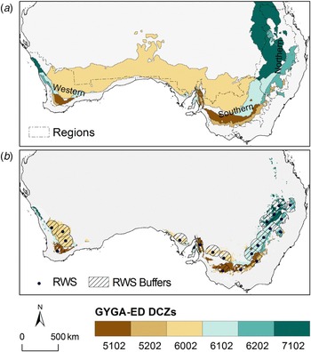
Designated climate zones for Yg analysis were identified following the GYGA protocol selection criteria of each zone containing at least 0·05 of total national crop area (Fig. 1(a) and (b)). Geographic information system (GIS) analysis (ArcGIS v10; ESRI 2010) was used to intersect the cereals land use layer (ABARE-BRS 2010) and GYGA-ED climate zones (Van Wart et al. Reference Van Wart, van Bussel, Wolf, Licker, Grassini, Nelson, Boogaard, Gerber, Mueller, Claessens, van Ittersum and Cassman2013b ). Both data sets were converted to an Australian Albers equal area projection (ESRI 2010) to enable land areas to be calculated.
(a) Global Yield Gap Atlas Extrapolation Domain (GYGA-ED) climate zones (CZ) which cover 5% or more of the Australia cereals zone, selected as designated climate zones (DCZ), and broad cropping regions (source: GRDC); (b) the six DCZs selected for analysis masked to show only cereal crop land use areas, plus the 22 reference weather stations (RWS) and their buffer zones. Colour online.

Weather station selection
A minimum of 10–15 years of weather data is recommended for Yg analysis of crops grown in variable rainfed environments and 15–20 years may be desirable to better account for year-to-year variation in weather (Van Wart et al. Reference Van Wart, Kersebaum, Peng, Milner and Cassman2013a ; Grassini et al. Reference Grassini, van Bussel, Van Wart, Wolf, Claessens, Yang, Boogaard, de Groot, van Ittersum and Cassman2015). There is a trade-off between using longer periods to better account for climate variability and shorter periods to avoid analysis being substantially affected by uptake of new technology and by climatic change (van Ittersum et al. Reference van Ittersum, Cassman, Grassini, Wolf, Tittonell and Hochman2013). A 15-year period (1996–2010) was used in the current study.
Grassini et al. (Reference Grassini, van Bussel, Van Wart, Wolf, Claessens, Yang, Boogaard, de Groot, van Ittersum and Cassman2015) advocate use of the best available weather data from sources which range from high-quality, long-term (>10 years) meteorological stations (Level 1), shorter term (⩽10 years) station data with missing periods infilled with generated data (Level 2), through to mostly or fully generated or gridded weather data (Level 3). Two main weather data sources are available for Australia. The Australian Bureau of Meteorology (BoM) manages a network of meteorological stations for which daily data are available. Within the wheat-cropping zone, the highest quality stations are 19 BoM stations that have recorded data sets covering rainfall, temperature and evaporation data for at least the previous 20 years, and correspond to Level 1 stations. In addition to the BoM data, 2562 Silo Patched Point Data set (PPD) sites were available, many of which are stations where limited variables are recorded (e.g. only rainfall) or provide incomplete temporal coverage and are in-filled with interpolated data from available nearby stations (Jeffrey et al. Reference Jeffrey, Carter, Moodie and Beswick2001). The PPD stations therefore correspond to Level 2 stations. Daily solar radiation is recorded at relatively few stations nationally and was sourced as interpolated data (Zajaczkowski et al. Reference Zajaczkowski, Wong and Carter2013) for both primary and secondary stations.
The GYGA protocol specifies the use of 100 km radius buffer zones around selected RWS. Selection of RWS aims to use the highest quality stations first, and to minimize the number of stations needed for estimation and overlap between adjacent RWS buffer zones while providing good coverage over the most important cropping regions. Selecting RWS buffer zones to cover 0.50 of national crop production area was found to produce robust Yg estimates where topography is relatively uniform (Van Wart et al. Reference Van Wart, Kersebaum, Peng, Milner and Cassman2013a ; van Bussel et al. Reference van Bussel, Grassini, Van Wart, Wolf, Claessens, Yang, Boogaard, de Groot, Saito, Cassman and van Ittersum2015).
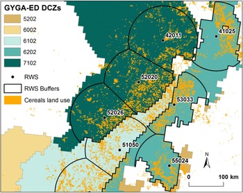
Following the GYGA protocol, RWS were iteratively selected within the DCZs in order to maximize the cereal crop area within the RWS buffer zones. Stations were ranked to select those with the greatest crop harvested area within their 100 km buffer zone, and were excluded if their buffers did not contain at least 0·01 of the national cropped area. As per the GYGA protocol, the selection of RWS in this Australian analysis used the available Level 1 stations first, and then the selection process continued using the PPD (Level 2) stations. A Python script tool for ArcGIS v10 (ESRI 2010) was developed to automate the iterative process of RWS selection. To prevent selection of buffers with substantial overlap, the GYGA protocol recommends excluding RWS if they are <180 km apart within a DCZ (corresponding to a circular buffer overlap of approximately 0·04). However, since the shapes of DCZs in Australia were not conducive to accommodating this restriction the proximity of RWS was not restricted, but instead RWS buffer zone boundaries were generated to remove all overlap (Fig. 2). Details of the 22 RWS selected are summarized in Supplementary Material 1 (available from http://journals.cambridge.org/AGS).
Illustration of the clipping applied to reference weather station (RWS) buffer zones. Buffers were clipped to climate zones (jagged boundaries) as per the Global Yield Gap Atlas (GYGA) protocol, then to avoid any overlap with adjacent RWS buffers, buffers were clipped to equidistant chords (straight boundaries). Colour online.

Quantification of water-limited yield
Estimation of Yw as per the GYGA protocol requires the use of crop simulation models and specifically should be undertaken with a model calibrated to local conditions (van Ittersum et al. Reference van Ittersum, Cassman, Grassini, Wolf, Tittonell and Hochman2013; Van Wart et al. Reference Van Wart, Kersebaum, Peng, Milner and Cassman2013a ). The APSIM modelling framework (Keating et al. Reference Keating, Carberry, Hammer, Probert, Robertson, Holzworth, Huth, Hargreaves, Meinke, Hochman, McLean, Verburg, Snow, Dimes, Silburn, Wang, Brown, Bristow, Asseng, Chapman, McCown, Freebairn and Smith2003; Holzworth et al. Reference Holzworth, Huth, deVoil, Zurcher, Herrmann, McLean, Chenu, van Oosterom, Snow, Murphy, Moore, Brown, Whish, Verrall, Fainges, Bell, Peake, Poulton, Hochman, Thorburn, Gaydon, Dalgliesh, Rodriguez, Cox, Chapman, Doherty, Teixeira, Sharp, Cichota, Vogeler, Li, Wang, Hammer, Robertson, Dimes, Whitbread, Hunt, van Rees, McClelland, Carberry, Hargreaves, MacLeod, McDonald, Harsdorf, Wedgwood and Keating2014) is well validated for Australian wheat crops (Keating et al. Reference Keating, Carberry, Hammer, Probert, Robertson, Holzworth, Huth, Hargreaves, Meinke, Hochman, McLean, Verburg, Snow, Dimes, Silburn, Wang, Brown, Bristow, Asseng, Chapman, McCown, Freebairn and Smith2003; Hochman et al. Reference Hochman, Holzworth and Hunt2009; Carberry et al. Reference Carberry, Liang, Twomlow, Holzworth, Dimes, McClelland, Huth, Chen, Hochman and Keating2013; Brown et al. Reference Brown, Huth, Holzworth, Teixeira, Zyskowski, Hargreaves and Moot2014) and has been previously applied to Yg assessment in Australia (Hochman et al. Reference Hochman, Gobbett, Holzworth, McClelland, van Rees, Marinoni, Navarro Garcia and Horan2012; Oliver & Robertson Reference Oliver and Robertson2013). It is a daily time-step simulator incorporating meteorological data and sub-models for crop growth, soil water and nutrients. A large number of wheat varieties have been parameterized for APSIM and the model enables specification of flexible crop sowing and fertilizer application rules. Frost and extreme heat events may have significant impacts on grain crop yields, subject to the timing of these events in relation to crop growth stage. However, APSIM has limited ability to simulate these spatially variable and infrequent events (Barlow et al. Reference Barlow, Christy, O'Leary, Riffkin and Nuttall2015), which were not included in the simulations used in the current study. This is a known, but unavoidable and poorly quantified, source of overestimation of Yw in some cases.
Selection of soils
Following the principles of the GYGA protocol, soil characterizations providing the attributes required for crop modelling should be as locally relevant as possible and based on observed data if available. Only the major soil types utilized by a cropping system need to be considered. Fourteen Australian Soil Classification (ASC) orders are defined for the Australian continent. Geographic information system analysis was used to select up to three soils from the dominant ASC soil orders for each RWS buffer, from national soil maps (ACLEP 2012). Only ASC orders that covered at least 0·05 of the cropped area within each RWS buffer zone were selected. Using this approach, the proportion of cropped soil areas within the RWS buffer zones represented by crop modelling ranged from 0·90 to 1·00.
The APSoil database (http://www.apsim.info/Products/APSoil.aspx; Dalgliesh et al. Reference Dalgliesh, Foale and McCown2009) contains over 1000 georeferenced and detailed soil characterizations suitable for simulations of Yw in Australia. Locally characterized soils from the APSoil database were matched with the ASC order, plant available water capacity (PAWC) and bulk density of the soils selected within the RWS buffer zones. An inherent assumption in using APSoil in this manner is that the soil sampling locations are representative of local soils of that type. A bias in soil samples towards better quality soils could lead to overestimation of Yw. The PAWC calculated for APSoil incorporates physical and chemical constraints that may restrict crop-rooting depth. Wheat PAWC for the selected soils ranged from a low of 61 mm for a deep sand at Wongan Hills, Western Australia to a high of 296 mm for a medium clay at Dunmore, Queensland (key data for the 22 RWS are summarized in Supplementary Material 1, available from http://journals.cambridge.org/AGS).
Agronomic management details
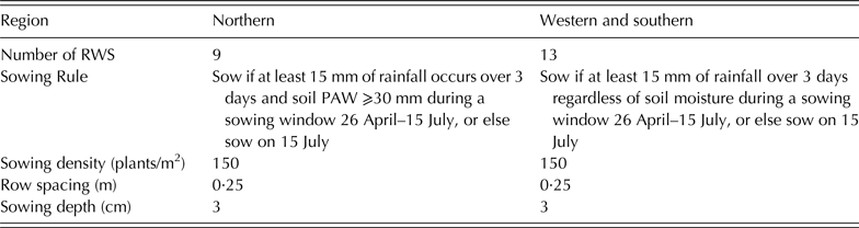
Crop simulations for each soil × RWS should use locally relevant agronomic management rules, however Grassini et al. (Reference Grassini, van Bussel, Van Wart, Wolf, Claessens, Yang, Boogaard, de Groot, van Ittersum and Cassman2015) acknowledge that cropping system details may not be readily available in many cases. For Australian wheat cropping systems, four highly regarded agricultural consultants from four states were surveyed to ascertain best practice, in relation to time of sowing, as reflected by their leading farmer clients. The survey responses revealed that best management practice is not easily characterized for simulating Yw. Generic sowing rules were defined based on local expertise, driven by rainfall and soil plant available water (PAW), which varied in detail depending on the cropping region (Fig. 1(a); Supplementary Material 1, available from http://journals.cambridge.org/AGS) in which each RWS was located (Table 1).
Generic sowing rules and parameters applied per region

RWS, reference weather stations; PAW, plant available water.
The current study assumed wheat–summer fallow–wheat–summer fallow rotations (cropping intensity = 1·0) as this is the most common sequence across the three cropping regions. For example, a Northern Australian grain zone survey showed an average cropping intensity of 0·94 (Hochman et al. Reference Hochman, Prestwidge and Carberry2014). For each RWS, an early-sown or late-sown variety (which in some cases was the same variety) was selected and used in all years of the simulation. These were selected from five wheat varieties chosen as representatives of progressively slower maturing types (early, mid-early, mid, mid-late and late). All five varieties were simulated over the 15-year period (1996–2010) for each soil type × RWS combination and the 15-year average yields for each were aggregated to RWS by weighting for the cropped area of each soil at each RWS. The early-sown variety selected for each RWS was the one with the highest 15-year average yield if sowing occurred between 26 April and 14 May, and the late-sown variety selected had the highest 15-year average yield if sowing occurred between 15 May and 15 July. The varieties chosen to simulate Yw for each RWS are listed in Supplementary Material 1, and the APSIM vernalization and photoperiod sensitivity parameters for the five maturity types are provided in Supplementary Material 2 (both available from http://journals.cambridge.org/AGS).
Grassini et al. (Reference Grassini, van Bussel, Van Wart, Wolf, Claessens, Yang, Boogaard, de Groot, van Ittersum and Cassman2015) highlighted that soil moisture content at time of crop sowing can have a large impact on Yw and that crop simulations should cover the entire period of interest. Since starting soil moisture conditions at each RWS were unknown, values were arbitrarily set for 1 January 1981 and continuous wheat–summer fallow–wheat simulations (where summer fallow extends from harvest in late spring–early summer through to sowing in the following autumn–winter period) were simulated from 1981 to 2010. The sequence of wet and dry seasons over 14 years of simulations from 1981 to 1995 were more than sufficient to allow any error in the initial setting of soil water to self-correct (setting the initial value too high will result in higher biomass production, which will simulate increased water use, while setting initial value too low will result in lower biomass production, which will simulate reduced water use). The Yw values simulated prior to 1996 were discarded from the Yg analysis calculations.
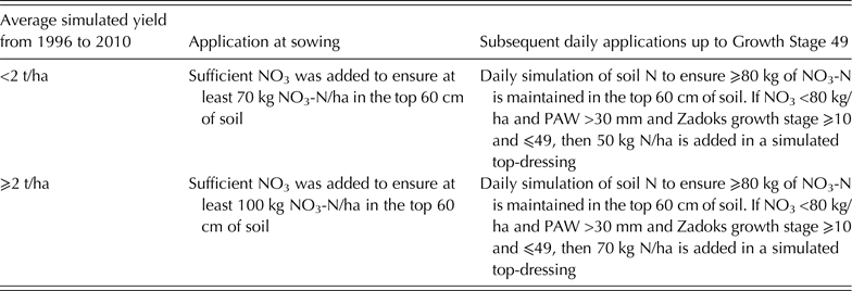
Nutrient availability, such as soil N, should be non-limiting in simulation of Yw (Grassini et al. Reference Grassini, van Bussel, Van Wart, Wolf, Claessens, Yang, Boogaard, de Groot, van Ittersum and Cassman2015). Unlike other crop models, it is not possible to disable the N module to simulate a nutrient unlimited yield in APSIM. This is because there are many dependencies between the soil N (SOILN), soil water (SOILWAT) and the surface organic matter (RESIDUE) modules. The RESIDUE module simulates crop residue on the soil surface that influences soil moisture loss through evaporation. With the N module disabled, soil surface residue breakdown will be affected, which in turn would affect the water balance. Instead of disabling the N module, fertilizer application rules were used (Table 2) to ensure at least 50 kg N/ha was available as nitrate (NO3-N) in the top 60 cm of soil, at the start of each day, up to the ‘first awns visible’ growth stage (GS), GS 49 (Zadoks et al. Reference Zadoks, Chang and Konzak1974). This means that soil N rarely limits crop yield. However, the problem of ‘haying off’ needs to be avoided – a situation where excessive vegetative growth leads to water stress during grain-filling, and results in lower yields (van Herwaarden et al. Reference van Herwaarden, Farquhar, Angus, Richards and Howe1998). These N application rules, with conditional in-crop application of N, were designed through iterative experimentation to make haying off very unlikely in dry springs, while minimizing the chance of N limiting yields in the most favourable springs. Sensitivity analysis with variations of the fertilizer rule with higher and lower rates of N (data not shown) provided confidence that these rules resulted in the best estimate of water-limited and N-unlimited wheat yields.
Fertilizer application rules used to ensure that N nutrition is non-limiting in simulation of water-limited wheat yields
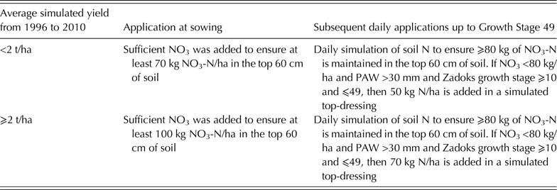
N, nitrogen; NO3, nitrate; PAW, plant available water.
Actual yield
The GYGA protocol indicates that Ya data should ideally be sourced from administrative units that are congruent with the RWS buffer zones, and where multiple administrative units occur within an RWS buffer, a weighted average by area should be calculated (Grassini et al. Reference Grassini, van Bussel, Van Wart, Wolf, Claessens, Yang, Boogaard, de Groot, van Ittersum and Cassman2015). The smallest administrative unit at which national agricultural data are collated by the Australian Bureau of Statistics (ABS) is the statistical local area (SLA). Censuses at SLA level are only carried out every 5 years, but annual surveys are reported at the coarser level of statistical division (SD) (Walcott et al. Reference Walcott, Zuo, Loch and Smart2013). Statistical divisions are relatively uniform regions with boundaries determined from socioeconomic criteria; SLAs are based on local government areas, and are subdivisions of SDs, averaging >30 SLAs per SD across the Australian cereals zone.
Data on annual crop yields for the 15 study years (1996–2010) were sourced from ABS (2012). Linear regressions were used to downscale yields (t/ha) from SD to SLA in non-census years (method described in detail in Supplementary Material 3, available from http://journals.cambridge.org/AGS). This provided Ya data for the 167 SLAs that were partially or completely included within the RWS buffer zones. Statistical local area level data were weighted by the cropped area of each SLA within the RWS and then aggregated to the RWS level.
Upscaling from reference weather station to national scale
The GYGA protocol outlines several steps for generating weighted aggregates from the crop simulations to RWS, DCZ and the national level (van Bussel et al. Reference van Bussel, Grassini, Van Wart, Wolf, Claessens, Yang, Boogaard, de Groot, Saito, Cassman and van Ittersum2015). The aggregation steps applied to Yw in the current analysis were:
-
1. For each RWS calculate Yw annually for each soil type;
-
2. Weight Yw per RWS per year by the fraction of crop area per soil type within the RWS buffer;
-
3. Add the weighted average annual Yw values for each soil type to derive an annual Yw value for each RWS;
-
4. Average 15 years of Yw per RWS to give 15-year average Yw per RWS.
-
5. Calculate the 15-year average Yw per DCZ, weighting each RWS by its fraction of the crop area within each DCZ.
-
6. Calculate the 15-year average national Yw, weighting each DCZ by its fraction of the national crop areas.
Annual RWS Ya values were aggregated to DCZ and national level using steps 4–6 in an equivalent manner. National Yg and Y% values were calculated from the 15-year average national Ya and Yw values.
Rainfall amount and variability
To examine the relationships between crop yields, Yg and rainfall, the mean annual effective rainfall (ER) was calculated. This approximates the total water available for rainfed crop growth by combining growing season rainfall (April–October) with a proportion of the rainfall from the preceding fallow period (November–March) (Eqn (1)). The fraction of fallow period rainfall available to a crop is known as the fallow efficiency. A wide range of fallow efficiency values have been reported in Australian studies (Freebairn et al. Reference Freebairn, Wockner, Lawrence, Cawley, Hamilton, Michalk and Pratley1998; Oliver et al. Reference Oliver, Robertson and Weeks2010; Hunt & Kirkegaard Reference Hunt and Kirkegaard2011; Whitbread et al. Reference Whitbread, Davoren, Gupta, Llewellyn and Roget2015). Nevertheless, the current study selected 25% as a plausible uniform figure for such a national analysis:
 $${\rm ER}\, = \,0 {\cdot} 25 \times \sum ({\rm Nov} - {\rm Mar \;rainfall}) + \sum ({\rm Apr} - {\rm Oct \;rainfall})$$
Effective rainfall was calculated from rainfall data records for each RWS weather station from 1960 to 2010, with this longer period used to determine a measure of historical long-term rainfall variability. Similarly, to investigate the relationship between crop yields and Yg and the variability of rainfall, ER variability was calculated as standard deviation (s.d.) and coefficient of variation (CV) of ER per RWS over the same period.
RESULTS
National yields and yield gap
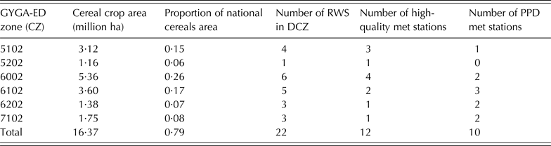
The six CZs selected as DCZs for analysis covered 0·79 of the total cereal cropping area (Fig. 1(a) and (b)) and individually covered from 1·16 million ha to 5·36 million ha (Table 3). Some important wheat cropping areas were excluded from the DCZs, including cropping areas in both low and high rainfall zones, such as parts of the Western Australia Wheat Belt, South Australian Eyre Peninsula and Victorian Mallee. The 22 RWS buffer zones cover 0.52 of the national cereals area (Fig. 1(b)). Twelve of the 22 RWS were high-quality (Level 1) stations, while the remaining ten weather stations (PPD meteorological stations) were Level 2 stations. Each DCZ included at least one high-quality weather station (Table 3). While the GYGA protocol supports using lower grade weather data or inclusion of additional CZs with <0·05 of the national crop area if adequate crop area coverage is not achieved, neither option was necessary in this case.
Area and proportion of national cereal crop area covered by the six DCZs, and a summary of the quality of RWS used within the DCZs

DCZ, designated climate zone; RWS, reference weather stations; GYGA-ED, Gap and Water Productivity Atlas Extrapolation Domain; CZ, climate zone; PPD, Patched Point Data set.
The approach used in the current study, of clipping the boundaries of adjacent RWS buffers within DCZs, rather than simply excluding any RWS <180 km apart as per the GYGA protocol, resulted in selecting some RWS as close as 135 km apart within the same DCZ. However, this method ensured that no crop area was double-counted (Fig. 2).
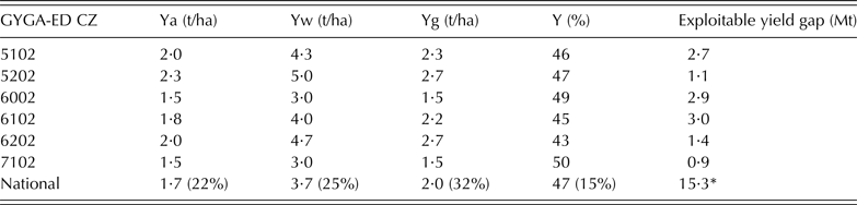
Interestingly, GYGA-ED climate zone 6002, which encompasses the largest proportion of cropping area, also includes extensive proportions of arid and semi-arid rangelands, not suited to cropping of any type (Fig. 1(a)). The cereal cropping in this zone is the most marginal and shows the lowest Ya (1·45 t/ha) and Yw (2·95 t/ha) of the six zones. Zone 5202, which covers the smallest proportion of national crop area (0·06) has the highest Ya (2·33 t/ha) and Yw (4·99 t/ha) of the six zones (Table 4).
Summary of farmer yields (Ya), water-limited yield potential (Yw), national yield gap (Yg) and relative yield (Y%) estimates at designated climate zone (DCZ) and national levels

Numbers in brackets are the coefficient of variation (from reference weather stations). The exploitable yield gap represents additional wheat yield in millions of tonnes (Mt) that would be harvested if Ye (80% of Yw) is achieved over the Australian wheat crop area (average 1996/97 to 2010/11) of 12·3 million ha (ABARES 2012).
GYGA-ED, Gap and Water Productivity Atlas Extrapolation Domain; CZ, climate zone.
* The national exploitable yield gap is based on average national wheat cropping areas (1996/07 to 2010/11; ABARES 2012), not just the wheat cropping areas in the six DCZs.
The aggregated outputs from the application of the GYGA protocol (Table 4) scaled up nationally to a Ya of 1·73 t/ha and a Yw of 3·72 t/ha. The calculated national Yg was 1·99 t/ha and the overall Y% was 47%. The scaled-up Ya compares closely to a national Ya of 1·70 t/ha, calculated by dividing the average total wheat production for 1996/2007 to 2010/11 (20·9 million t) by the average crop area of 12·3 million ha (ABARES 2012).
Applying these GYGA protocol results to the total national wheat cropping area, if Australian farmers improved production to achieve a Y% of 80% from existing rainfed wheat cropping areas, the 72% increase in production would equate to an additional 15·3 million t of wheat (Table 4). In financial terms, with a wheat price of US$ 212 per t (based on Chicago Board of Trade price for contract delivered July 2015, sourced 9 July 2015), this additional export would be valued at US$ 3·2 billion per year.
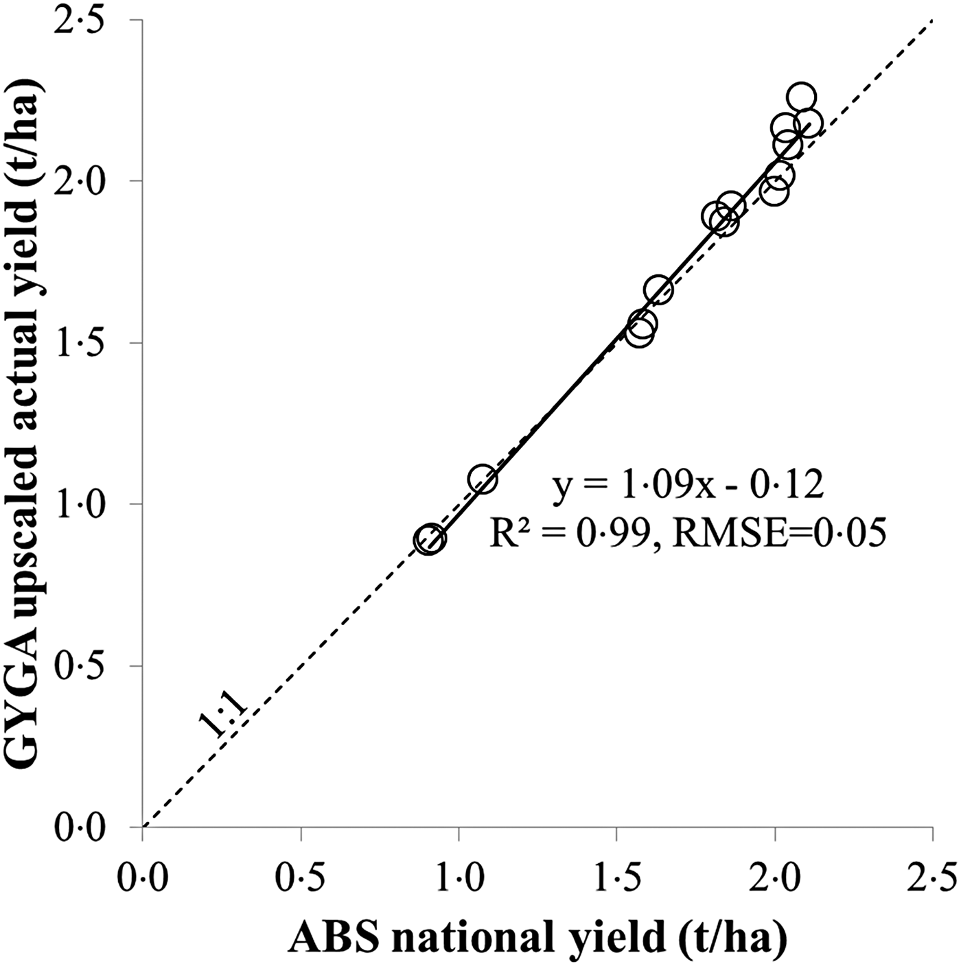
The Ya data are an important input into the Yg calculations. The process of generating annual Ya estimates at SLA level, then proportionately associating SLA yields to RWS and upscaling to national level compared well with the national annual average wheat yields from the aggregated annual national ABS data (Fig. 3), which are based therefore on the whole national wheat cropping area. While the overall agreement is exceptionally good, especially given that only 0·52 of the area was sampled, a slight overestimation of Ya under the GYGA protocol was evident in the four highest yielding years, which may lead to a small underestimation of Yg in those high-yielding years.
Farmer yields (Ya) derived from Global Yield Gap Atlas (GYGA) protocol upscaling plotted against national average annual wheat yields (ABS 2012) for the 15 study years (1996–2010). The dotted line represents a 1-to-1 relationship, and the solid line is a fitted trend line with the regression equation, R 2 and residual mean-square error (RMSE) shown.

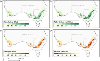
In maps of the results aggregated to DCZ and masked to show only the cereal cropping areas (Fig. 4), Ya and Yw follow similar distributions, with lower yields in the warmer and drier inland areas. Similarly, Yg tends to be lower in the less productive areas, and higher in the more productive and higher rainfall areas. Conversely, Y% tends to display a reverse pattern compared with Yg, with higher Y% in lower yielding DCZs, and lower Y% in higher yielding zones. These relationships are explored further below.
Maps showing results for designated climate zones (masked to cereal areas) (a) farmer yields (Ya), (b) water-limited yield potential (Yw), (c) yield gap (Yg) and (d) relative yield (Y%). Dashed lines indicate Australian state boundaries. Colour online.

Analysis of the components of yield gaps and their correlation with reference weather station effective rainfall
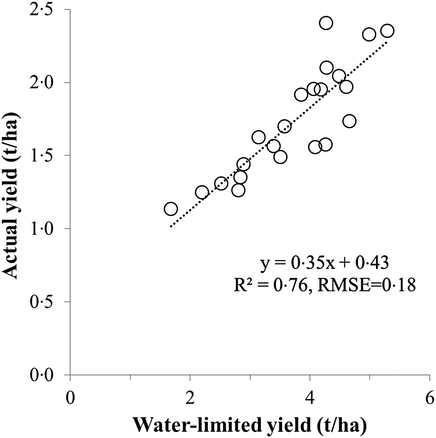
The correlation between average RWS Ya and Yw values provides some insights into the nature of the Australian Yg. Simulated Yw values are highly correlated with the surveyed Ya values (Fig. 5). The slope of the regression line, being <1, implies that the Yg increases as Yw increases. Correspondingly, the Y-axis intercept of this plot being >0 shows that Y% is lower at RWS with higher Yw.
Relationship between 15 year average actual yields (Ya) and water-limited yield potential (Yw) of all reference weather stations (RWS). Dotted line is a fitted linear function significant at P < 0·001.

Fifteen-year trends in yields and yield gaps
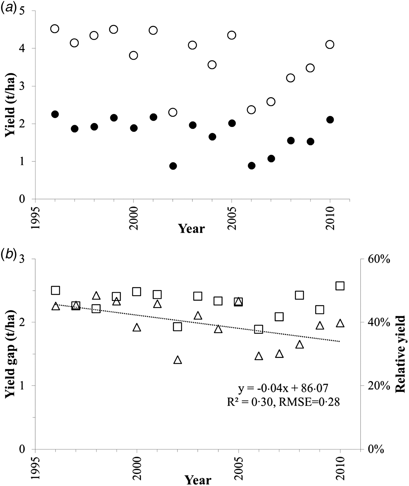
There is marked year-to-year variation in national Ya, Yw and Yg. Actual yield values ranged from 0·9 to 2·3 t/ha and Yw ranged from 2·3 to 4·5 t/ha, with low-yielding years associated with droughts that affected major wheat growing areas, especially in 2002, 2006 and 2007. On a year-to-year basis, over the 15 years, national average Yw is a strong predictor of Ya (R 2 = 0·96; residual mean-square error (RMSE) = 0·087 t/ha; P < 0·001). National yield gap ranged from 1·4 t/ha in 2002, a drought year, to 2·4 t/ha in 1998, a moderate yielding year. Relative yield values ranged from 38% in 2002 to 51% in 2010 (a moderately high yielding year).
Both Ya and Yw showed highly variable annual values over the 15-year study period (Fig. 6(a)) with no significant effects at P < 0·05. However, Yg shows a significant decrease (P < 0·05), with the regression showing an average reduction in the Yg of 42 kg/ha/year (R 2 = 0·30, RMSE = 0·28 t/ha) over the study period (Fig. 6(b)). Relative yield did not show a statistically significant effect and is a remarkably consistent index, despite highly variable seasonal conditions (Fig. 6(b)).
National annual yields and yield gaps (Yg) over the 15-year study period (a) farmer yields (Ya)  and water-limited yield potential (Yw)
 (b) yield gap (Yg)
 and relative yield (Y%)
 with a trend line fitted to Yg.

Correlation of yield gaps and their components with reference weather station average effective rainfall and rainfall variability
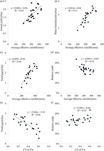
Average effective annual rainfall, represented by ER (Eqn (1)), varied from 200 to 428 mm over the 50-year period (1960–2010) across the 22 RWSs, and the CV of ER varied from 0·19 to 0·36. This longer period was chosen to reflect longer-term farmer memory of climatic variability than would be captured in the 15 years of the study period. Both Ya and Yw correlate significantly with ER (Fig. 7(a) and (b)). Of the two yield gap measures, Yg shows a strong relationship with ER. The correlation of Y% with ER is negative, and although weaker, it is also significant (Fig. 7(c) and (d)). These results clearly, and unsurprisingly, demonstrate that yields and yield gaps are strongly influenced by rainfall available to crops in such rainfed cropping environments. The negative correlation of Y% with ER suggests that farmers in lower rainfall environments may be achieving more of their Yw than those in higher rainfall environments (see also Figs 4(d) and 5).
Relationships of reference weather station average yield and yield gap measures to average effective rainfall (ER), calculated over the period 1960–2010 and to coefficient of variation (CV) of water-limited yield potential (Yw) over the 15 year study period. (a) farmer yields (Ya) and ER, (b) Yw and ER, (c) yield gap (Yg) and ER, (d) relative yield (Y%) and ER, (e) Yg and CV of Yw, (f) Y% and CV of Yw. Regressions in a, b, c and e are significant at P < 0·001, d is significant at P < 0·01 and f is significant at P < 0·05.

Surprisingly however, RWS average Ya did not correlate with long-term variability in ER as indicated by either the s.d. or CV of ER, or with other measures of year-to-year variability such as the mean annual change (mean of n−1 absolute values of year-to-year differences of ER) or lag-one correlation of ER (results not shown). Likewise, both Yg and Y% did not correlate with the CV of ER (results not shown). In contrast, the CV of Yw, calculated for each RWS over the 15 study years, did correlate with yields and yield gap measures. Actual yield correlated significantly with CV of Yw (R 2 = 0·59, P < 0·001) as did Yw (R 2 = 0·74, P < 0·001) (results not shown). These results confirm that sites with higher Ya and Yw (and higher rainfall) are also sites with lower variability. It is consistent therefore that Yg also shows a negative relationship with CV of Yw (Fig. 7(e)), indicating larger yield gaps at sites with lower variability. Surprisingly, the relationship between Y% and CV of Yw (Fig. 7(f)) indicates that sites with lower variability and higher yields are not achieving yields as close to Yw as sites with lower rainfall and higher variability.
DISCUSSION
Australian wheat yield gap
A key finding of the current analysis is the substantial national Yg for Australian rainfed wheat cropping of nearly 2 t/ha. Expressed as a Y% of 47%, this result indicates that Australian farmers consistently produce less than half of the water-limited wheat yields achievable with yield-maximizing management practice. This estimate is lower than, but broadly supported by, other yield gap studies within Australia. The broadest scale studies showed mean water use (production) efficiencies of 52% (1996–2000) and 51% (2003–08) across 14 agro-ecological zones (Stephens et al. Reference Stephens, Anderson, Nunweek, Potgieter and Walcott2011). At state level, Fischer et al. (Reference Fischer, Byerlee and Edmeades2014) showed a Y% of 69% for the Western Australia wheat belt in 2010. A regional estimate of 52% for the Wimmera in Southeastern Australia over 20 years (Hochman et al. Reference Hochman, Gobbett, Holzworth, McClelland, van Rees, Marinoni, Navarro Garcia and Horan2012) is also comparable. Similar results were also obtained in an analysis of district yields (Wagga Wagga, New South Wales) which estimated that actual yields were less than half of potential in 19 of 25 years from 1960 to 1984 (Cornish & Murray Reference Cornish and Murray1989). A Y% estimate of 65% in Australia's northern grain zone (Hochman et al. Reference Hochman, Prestwidge and Carberry2014) was based on surveys of farmers who retained detailed farm records, which probably excluded some of the less progressive farmers, so may not reflect the national average. These previous national and regional studies indicate that the national Y% result obtained in the current work is robust.
The Y% figure of 47% derived for Australia is somewhat lower than those reported for other countries, including rainfed wheat in Germany (1986–2008) at 80% (Van Wart et al. Reference Van Wart, Kersebaum, Peng, Milner and Cassman2013a ); nine locations in India at 63%; and two locations in Mexico at 71% (Lobell et al. Reference Lobell, Cassman and Field2009). Fischer et al. (Reference Fischer, Byerlee and Edmeades2014) report a world average Y% of 67% estimated for 2008–2010. Studies have reported high Y% for some Australian wheat farms, such as a study of leading growers nationally (2004–08), who were users of the Yield Prophet® decision support system, with Y% of 77% (Hochman et al. Reference Hochman, Holzworth and Hunt2009). Another study of three farmers, who have been early adopters of decision support tools, and of best management cropping practices over 16–20 years showed Y% of 74–82% (van Rees et al. Reference van Rees, McClelland, Hochman, Carberry, Hunt, Huth and Holzworth2014). These outcomes provide encouraging evidence that national yield gaps may potentially be reduced to 0·75–0·80 of Yw using existing best practice crop management and currently available varieties. The actual achievement of this target would require a major investment in education and extension to reach and transform the practices of the less productive grain growers.
The current study estimates a potential to increase production by 15·3 million t if the entire national wheat area were to achieve Y% of 80%. With an export value of US$ 3·2 billion/year, this additional yield is not only substantial in financial terms, but highlights the potential for Australia to make a more substantial contribution to achieving global food security by providing a buffer for annual fluctuations in global and regional yields.
Evaluation of the Global Yield Gap Atlas protocol
The current study is a first attempt to apply a consistent global protocol to assess Australian national wheat yield gaps. The GYGA protocol uses a tiered approach to data selection by deploying the best available local data and upscaling from the local to the national levels. Given the wide spatial and temporal variability of cropping conditions, this Australian analysis is a challenging test case of the implementation of the GYGA protocol. The local and global relevance of GYGA could be compromised if the underlying data are inaccurate, or if an unsuitable crop model is deployed, or if the approach of upscaling from RWS to DCZ to national level is inappropriate. However, Australia generally has good quality production data, with the weather and soils data used in the current analysis being of high quality, and the agronomic rules and the APSIM crop model are well validated for use in Australian wheat cropping systems. Comparison of the Australian Ya data with ABS national yield data demonstrated that the GYGA protocol method of upscaling from RWS buffer to national level has resulted in the calculation of a Ya value that was consistently close to the national average for the entire wheat cropping area, sourced from the national agricultural statistical service, ABARES. This demonstrates the validity of GYGA's upscaling methodology. Furthermore, comparing the results of the current analysis with previous national and regional studies shows that the GYGA protocol is a robust approach for estimating yield gaps at a national scale.
Factors influencing yield gaps
An important challenge is to identify where greatest yield gains can be made with a reasonable degree of certainty. The slope of the fitted regression line between Ya and Yw is <1, which indicates that Ya falls further behind as Yw increases. The current analysis has also demonstrated that Yw is a strong predictor of Ya, both on a site-by-site basis, as well as on a year-to-year basis nationally. The related observation that Y% is higher in areas with lower Yw and greater variability of Yw, may be driven by different factors in low- and high-yielding areas. In lower yielding areas, farmers may on average be making more finely tuned management decisions, and therefore achieving yields that are closer to their Yw. High-yielding areas tend to be more susceptible to yield losses due to weeds, pests, diseases and potential for waterlogging and the subsequently higher costs and risks of production. Assuming that the APSIM simulations provide a robust reflection of Yw, the potential gains in yields from reducing the Yg are greater where yields are currently higher. Anderson (Reference Anderson2010) made a similar point comparing several sites in Western Australia, suggesting that management most limits productivity in environments with higher rainfall, and also that the greatest scope for improving grain yields is in improving crop management to fully utilize rainfall in higher rainfall years. Understanding whether this relationship is unique to Australian rainfed wheat cropping, or extends to other modern large-scale crop production systems, and its key driving factors could provide insight for future research and development efforts to reduce yield gaps globally.
One unexpected finding from the current study comes from the analysis of trends over the 15-year period from 1996 to 2010. The analysis shows a reduction in Yg in the order of 42 kg/ha/year, although Y% did not change significantly in the same time. Whilst a decline in Yg is a positive change, the stability of Y% conflicts with this finding. In modern farming systems, ongoing technological improvements (e.g. genetics and farming practices) are expected to bring increases in Ya and therefore reductions in Yg. Scenario modelling to explore Australia's future (CSIRO 2015) has utilized a baseline trend of 1·0% growth in crop yields per annum, as well as higher production growth scenarios with 2·8% growth in crop yields per annum. However, in contrast to those projections, Ya does not appear to have increased over the 15 years of the current study. The relatively short period of the current analysis, compared with the year-to-year variability in yields, needs to be considered when interpreting these results.
Another surprising finding in the current study is that neither actual yields nor relative yields are related to the s.d. or CV of ER. This could be interpreted as showing that Australian wheat farmers’ crop management is not substantially influenced by rainfall variability, yet intuitively, farmers in areas exposed to greater climatic risk may be more conservative in decision-making and, consequently, lower yields could be expected where climatic risk is greater. Yield gaps are negatively related to variability in Yw, with lower yield gaps where variability is higher. Surprisingly, sites with higher variability also show higher relative yields. This further supports the finding that gains in addressing yield gaps are most likely to be made where yields are higher (and variability is lower). It is commonly stated that managing climate variability and business risk in low rainfall areas is a substantial challenge (van Rees et al. Reference van Rees, McClelland, Hochman, Carberry, Hunt, Huth and Holzworth2014; Whitbread et al. Reference Whitbread, Davoren, Gupta, Llewellyn and Roget2015). Additionally, a study in the Southern Australian wheat zone (Monjardino et al. Reference Monjardino, McBeath, Ouzman, Llewellyn and Jones2015) found that risk-aversion was likely to be an important factor in farmer N application rate decisions, and thus individual farmer attitudes to risk is a key determinant of yield gaps. This counterintuitive result is not easy to explain. The result may reflect that all of the sites in the current study occur in areas with such variable rainfall that growers’ responses to rainfall variability is only one risk factor driving farmer decision making. Additionally, important variable factors that affect farm profit (e.g. inputs costs and crop price variability) may also obscure the importance of rainfall variability as a risk factor. For example, the economic risk associated with failing to exploit potential yields in higher yielding sites may be greater than in lower yielding sites. Alternatively, farmers may be managing cropping risk through diverse ways not necessarily expressed in production results, for example, some farmers may adapt to risk by introducing higher productivity innovations and technologies, whereas others adopt low-input strategies in order to reduce financial risk (Feldman et al. Reference Feldman, Thomas, Farre Codina, Plunkett and Kingwell2015).
Global Yield Gap Atlas Extrapolation Domain zones at crop production margins
A globally applied agroclimatic zonation scheme is central to the GYGA protocol and the GYGA-ED zones (Van Wart et al. Reference Van Wart, van Bussel, Wolf, Licker, Grassini, Nelson, Boogaard, Gerber, Mueller, Claessens, van Ittersum and Cassman2013b ) were selected for this analysis. An important benefit of using a globally consistent agro-climatic zonation for a national analysis is that it may facilitate comparisons of yields and yield gaps among countries. Having a common methodology may help understanding of the potential contributions towards meeting global food demand that can be made by focusing research, development and extension efforts in these countries. The variables used to define the GYGA-ED zones, GDD and aridity index, are categorized into ten intervals which each contain equal proportions of global land areas growing at least one of the ten most important food crops (as per SPAM crop distribution maps (You et al. Reference You, Crespo, Guo, Koo, Sebastian, Tenorio, Wood and Wood-Sichra2009). A consequence of this approach is that marginal GYGA-ED zones at extreme limits of GDD and aridity, where cropping area density may be more sparse, may cover a wider range of agro-climatic conditions than the non-marginal zones, because cropping in those areas tends to be more sparsely distributed.
In this Australian analysis, DCZ 6002 is a marginal zone and although it contains the largest wheat crop area of any of the six DCZs, the majority of the zone is semi-arid or arid and is not suitable for cropping. In generating Yw estimates during the current analysis, it was found necessary to revise the source of weather data for the Kyancutta RWS, which is close to a climatically determined ‘hard edge’ of the cropping zone (Nidumolu et al. Reference Nidumolu, Hayman, Howden and Alexander2012) that is not captured in the GYGA-ED zonation scheme. The initially selected RWS (a Level 1 station) was not sufficiently representative of the surrounding cropped area, and follow-up analysis identified a more suitable Level 2 station nearby (Warramboo). In implementing the site selection steps outlined in the GYGA protocol (van Bussel et al. Reference van Bussel, Grassini, Van Wart, Wolf, Claessens, Yang, Boogaard, de Groot, Saito, Cassman and van Ittersum2015), it is therefore important to be mindful that the highest quality weather stations are not necessarily the most locally representative, and thus initial estimates of Yw should be vetted as a quality control step. This may especially apply to marginal CZs in which crop area distribution is not even throughout, such as zone 6002. The aim is to identify weather stations which best represent the cropping areas within the CZ, and following the protocol steps without some vetting may not always achieve this.
CONCLUSIONS
The present paper describes the first nationwide assessment of wheat yield gaps in Australia that was based on a globally recognized and internationally peer-reviewed methodology. The current study implemented the GYGA protocol, so that results may be compared in a global context. The results presented are consistent with the results of other Australian and international studies, and build confidence in the suitability of the methods outlined by the GYGA protocol as long as the results are scrutinized and ‘sensibility tested’. Australian wheat cropping areas cover a diverse and challenging range of environments and so present a robust test case for the GYGA protocol. As the GYGA protocol was developed to be robust in relatively data poor environments, this national analysis relied on only 22 weather stations and associated cropping zones. The finding that national Yw estimates derived using the protocol are a strong predictor of national Ya shows that these 22 well-chosen weather stations and their associated soils could be used for generating progressive in-season national yield forecasts.
Undertaking the current analysis has led to valuable insights. The national relative yield figure of 47% indicates that Australian farmers have produced less than half of the water-limited yields achievable under yield-maximizing management practice, whereas van Rees et al. (Reference van Rees, McClelland, Hochman, Carberry, Hunt, Huth and Holzworth2014) demonstrated that leading farmers are capable of 74–82% over extended periods. This implies there is potential for Australian farmers to increase wheat yields substantially using available technologies. The results of the current study also show a reduction in the yield gap over the 15-year study period, but the relative yield remained stable over the period so the evidence for progress over this 15 year period is inconclusive.
The analysis of the role of rainfall and rainfall variability presented in the present paper demonstrates the potential application of outputs from yield gap analysis. At the scale of this study, yields and yield gaps are higher where rainfall is higher. However, lower relative yields are associated with higher rainfall sites and those with less year-to-year variability in water-limited potential yield than at sites with lower rainfall, and higher variability. This counterintuitive result challenges current understanding of climatic risk in relation to yield gaps. Developing a better understanding of farmer decision-making and risk responses may be a key factor in moving towards reduced yield gaps globally. The GYGA protocol provides a consistent methodology that facilitates inter-crop and inter-country comparisons that may support further exploration of this important area.
SUPPLEMENTARY MATERIAL
The supplementary material for this paper can be found at http://dx.doi.org/10.1017/S0021859616000381
This project was funded by CSIRO Agriculture. Contributions of Ms Di Prestwidge (CSIRO Land and Water) and interactions with Dr Justin Van Wart (University of Nebraska-Lincoln) have greatly helped this work to progress and develop. We acknowledge valuable comments from Dr Rick Llewellyn and Dr James Hunt (CSIRO Agriculture), and two anonymous referees, one of whom provided an exceptionally detailed and insightful review.