1 Introduction
In 2004, Haller proposed a new theory to capture separation in unsteady, two-dimensional flows, based on a nonlinear Lagrangian approach. In his study, the Lagrangian view was introduced by defining material lines characterised by particular properties when they coincide with a separation profile. While the Lagrangian frame was not new when studying flow separation, in previous studies, the term ‘Lagrangian’ generally referred to the use of Lagrangian coordinates, which were found to be more appropriate than Eulerian variables to detect a velocity singularity in the boundary-layer equations (valid only in the limit where the Reynolds number
 $Re\rightarrow \infty$
). This approach was for example used in van Dommelen & Shen (Reference van Dommelen, Shen and Cebeci1982), Cowley, Van Dommelen & Lam (Reference Cowley, Van Dommelen and Lam1990) and Degani, Walker & Smith (Reference Degani, Walker and Smith1998), among many other studies, even if an Eulerian counterpart can also be derived (Elliott, Smith & Cowley Reference Elliott, Smith and Cowley1983). Unfortunately, in flows where boundary layers are not sufficiently developed, or in moderate Reynolds number flows, these studies cannot apply.
Another well-known separation criterion is the Moore–Rott–Sears (MRS) principle, derived by Rott (Reference Rott1956), Sears (Reference Sears1956) and Moore (Reference Moore and Görtler1958). It stipulates that unsteady separation occurs at a location inside the flow where the shear stress vanishes. In practice, the velocity of that point has to be known, which is difficult or impossible to obtain. However, again, the MRS principle can be applied only in the context of high Reynolds number boundary-layer theory. On the contrary, in Miron & Vétel (Reference Miron and Vétel2015), an alternative was proposed to detect the off wall separation point by capturing a Lagrangian saddle point located on the most attracting material line extracted from the wall flow.
In his two-dimensional kinematic theory, Haller (Reference Haller2004) did not focus on the detection of the thickening of the boundary layer as in previous studies but instead defined the separation profile as a particular material line anchored at the wall that separates two different flow dynamics. Since any other line, either emanating from another point on the wall or from the true separation point but not coinciding with the separation profile (different slope), will be repelled in backward time towards the boundary, this provides mathematical arguments to extract the location and geometry of the instantaneous separation profile.
To our knowledge, only one experimental validation has been performed. Weldon et al. (Reference Weldon, Peacock, Jacobs, Helu and Haller2008) studied the separation induced by the rotation of a cylinder close to a solid wall. By adding a translation velocity profile parallel to the wall, an unsteady separation can be manipulated in various ways (in Hackborn, Ulucakli & Yuster Reference Hackborn, Ulucakli and Yuster1997, the cylinder is fixed and one of the wall is moving). For example, under periodic, quasi-periodic and random forcing, flow visualisations reveal that the separation profile moves in time but is anchored at a fixed location on the wall, in agreement with the theory of Haller (Reference Haller2004). However, to more precisely predict the slope of separation, numerical simulations were used to provide quantitative data instead of measured quantities.
The data required by the theory are indeed challenging to obtain. To compute the slope of the separation profile, knowledge of the first and second wall-normal derivatives of both velocity components is required. Expressed as wall quantities, the separation slope can be written as a function of the instantaneous wall shear stress, as well as streamwise derivatives of this quantity and of the pressure. These wall quantities are not easy to obtain, but the difficulty is all the greater because of the spatial resolution. Even in the apparently simple steady case, the Prandtl criterion stated that separation occurs where the skin friction point vanishes. At this singular point, velocity components and all spatial derivatives of the first order are null, so that higher-order derivatives have to be estimated inside a local region where very small velocities have to be measured and then differentiated in space, which moreover amplifies the experimental noise.
Another limitation of using only flow visualisations is that in Weldon et al. (Reference Weldon, Peacock, Jacobs, Helu and Haller2008), it was not possible to observe what happens when the amplitude of oscillations, in the periodic case, is significantly increased. Indeed, the authors argue that a material spike should not emanate from the wall since the cylinder spend only little time at a given location.
The objective of this study is to complete and extend the work performed by Weldon et al. (Reference Weldon, Peacock, Jacobs, Helu and Haller2008). Based on a set-up of the rotor-oscillator flow presented in § 2, we use particle image velocimetry (PIV) and extract required quantities to validate experimentally the theory of Haller (Reference Haller2004) without using numerical data, which is achieved for fixed separation in the periodic case in § 3. As our set-up allows large displacements of the cylinder, we investigate first in § 4 the case of moving separation where the flow is no longer periodic, before covering some intermediate flow conditions, including large periodic oscillations, in § 5. In this last section, a more practical example, the case of the impinging jet, is also treated to make a parallel with the rotor-oscillator flow.
2 Experimental set-up and measurement techniques
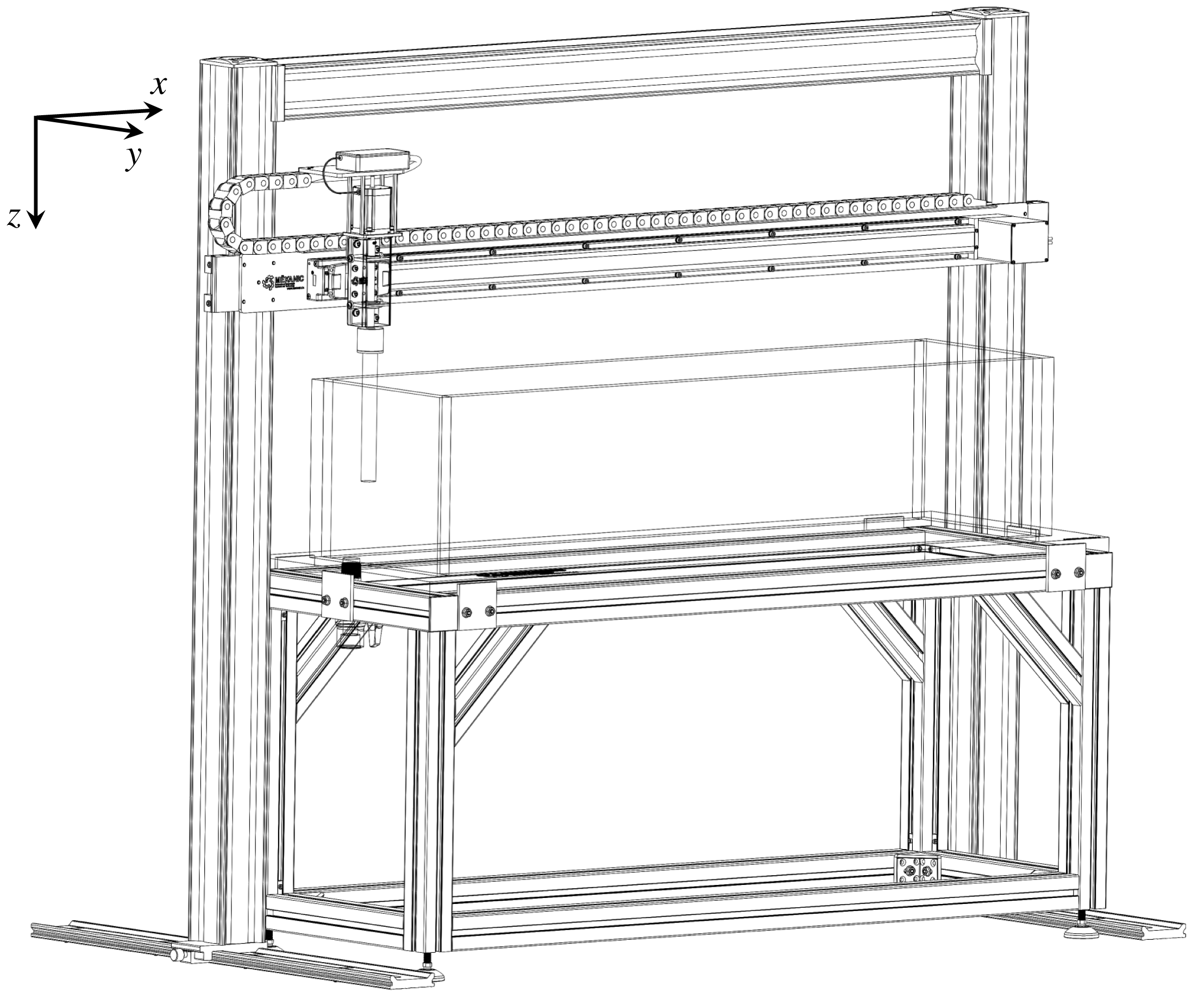
The experimental apparatus was designed to generate a rotating-oscillating movement of a cylinder inside a polymethyl methacrylate (PMMA) tank, as shown in figure 1. Both movements are assured by stepper motors: an anodised aluminium cylinder (
 $D=2.54$
cm,
 $L=30$
cm) is coupled to the first stepper motor shaft while being attached to a 130 cm linear motion rail controlled by the second motor. Use of stepper motors allows versatile options for the cylinder’s velocity
 $U_{c}$
while perfectly tracking its position. Five types of movements are studied: stationary rotation (no linear motion), steady translation, periodic oscillation, translation oscillation and smooth deceleration. All movements are added to the cylinder’s rotation. Smooth deceleration is produced by imposing a hyperbolic tangent velocity variation in time, while other motions are of the form
 $$\begin{eqnarray}U_{c}(t)=U_{0}+\unicode[STIX]{x1D6FD}\cos (2\unicode[STIX]{x03C0}ft),\end{eqnarray}$$
where
 $U_{0}$
is a constant translating velocity superposed on an oscillation of amplitude
 $\unicode[STIX]{x1D6FD}$
and frequency
 $f=1/T$
. For the periodic case,
 $U_{0}=0$
. The PMMA tank (
 $30~\text{cm}\times 30~\text{cm}\times 127$
cm) was filled with a 95 % glycerol, 5 % water by weight mixture seeded with fluorescent dye (Rhodamine B,
 $10~\unicode[STIX]{x03BC}\text{m}$
mean particle size). The water proportion was chosen in order to match the dye density and provide a uniform particle distribution. At
 $\unicode[STIX]{x1D6FA}=60$
rpm, the Reynolds number
 $Re$
, based on the cylinder–wall distance and the circumferential velocity of the cylinder, was
 ${\sim}5$
. When a translation motion is added, its value, based on the maximum velocity in the flow and the same distance, can increase up to
 $Re=20$
.
Three-dimensional assembly of the rotor-oscillator set-up.

Two-component PIV measurements were performed in a
 $xy$
plane half-way between the tank bottom plate and the free surface to avoid three-dimensional flow effects. The cylinder was positioned between
 $H=D$
and
 $H=2D$
away from the tank side wall depending on the case studied (see figure 2). Fluid illumination was created with a Nd : YAG 1200 mJ per pulse laser at a wavelength of 532 nm and a 4 ns pulse duration. A good trade-off between image resolution and field of view was achieved by positioning two CCD cameras side by side (LaVision Imager sCMOS, 5.5 megapixels equipped with a 60 mm focal length Micro-Nikkor lens) underneath the tank, perpendicular to the bottom plate. A maximal
 $25~\text{cm}\times 11$
cm field of view could be used when needed. The two images were merged and scaled with an appropriate calibration. The optics were equipped with a 550 nm long pass orange filter to emphasise the light reflected by the dye particles by raising the images contrast and to filter the laser reflections on the tank wall.
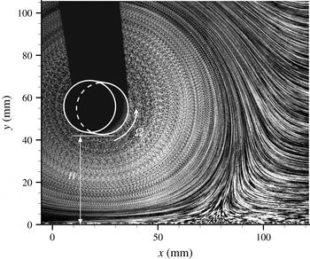
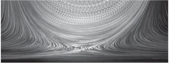
Flow streamlines from the stationary cylinder case (
 $U_{c}=0$
,
 $\unicode[STIX]{x1D6FA}=60$
rpm) revealed by PIV images averaged over a long period of time. The tank side wall is located at
 $y=0$
, on which a flow separation is observed at
 $x\simeq 75$
mm. Cylinder’s position and rotation are highlighted by the white circles. Black areas in the figure upper left part are shadows caused by the laser sheet coming from the bottom. Reflexion of particles is also observed on the bottom right side of the cylinder, manifested by a dark blur.

PIV raw images were also used for flow visualisation purpose. Snapshots were averaged over a certain period of time (from a few time steps to a long period, depending of the case) so as to represent the flow path lines. Such a case is for example showed in figure 2 for the stationary cylinder (
 $U_{c}=0$
).
The commercial software Davis 8.2 is used to process raw images. The cross-correlation is realised using a multi-pass process. The first iteration is performed on
 $64\times 64$
pixels windows. Then, three other passes are realised on
 $32\times 32$
pixels windows using a circular Gaussian weighting function and an overlap of 50 %. A post-processing step is finally performed to eliminate aberrant vectors, which normally affects less than 2 % of the vectors of the measurement domain, and are replaced by the median velocity of the neighbouring vectors.
Since most of cylinder motions were periodic (in an appropriate reference frame), velocity vector fields were phase averaged to reduce random errors. However, as many high-order spatial derivatives and temporal integrations have to be estimated to compute the separation profiles over time (Haller Reference Haller2004), results may be very sensitive to the remaining noise, and a more specific data treatment was required. As evoked in § 1, velocities at the wall are very low, especially in the vicinity of a separation point. To improve the quality of data, a bivariate polynomial of quintic order, obtained with a least-square fit, was used to approximate the velocity components in a region centred on the separation point. To estimate the accuracy of the results that can be deduced from this procedure, the analytical Stokes flow induced by a rotating and oscillating cylinder close to a wall given in Miron & Vétel (Reference Miron and Vétel2015) was used to compute the separation profile with exact velocity derivatives. Then, random errors, based on estimations of PIV velocity uncertainties (
 ${\sim}2\,\%$
of the maximum velocity), were added to the discrete velocity fields and the resulting data were treated with the procedure used for measured velocity fields. The uncertainty on the separation angle was then estimated to be less that 5 %, which was considered to be acceptable.
3 Fixed separation
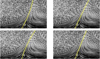
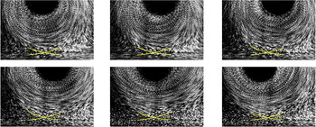
As preliminary results, figure 3 shows raw particle images phase averaged for the periodic case. By using corresponding phase-averaged velocity vector fields, the location of the fixed separation point was first detected where the wall shear stress, averaged over one oscillation period, vanishes. Then the unsteady separation profile (yellow line) was computed for each time step. The second-order profile is shown, which means that the slope and the curvature were obtained; this required to compute the spatial derivatives of the velocity vector (two components) at the separation point up to third order (Haller Reference Haller2004).
Visualisation of separation for the periodic flow (
 $\unicode[STIX]{x1D6FA}=60$
rpm,
 $\unicode[STIX]{x1D6FD}=5.7~\text{cm s}^{-1}$
and
 $f=0.4~\text{Hz}$
) with
 $H=2D$
. Particle images are phase averaged over 15 periods, and the yellow line is the theoretical second-order separation profile (Haller Reference Haller2004). Time elapses from left to right and from top to bottom, with a time delay of
 $T/4$
(see also supplementary movie 1 available at https://doi.org/10.1017/jfm.2018.188).

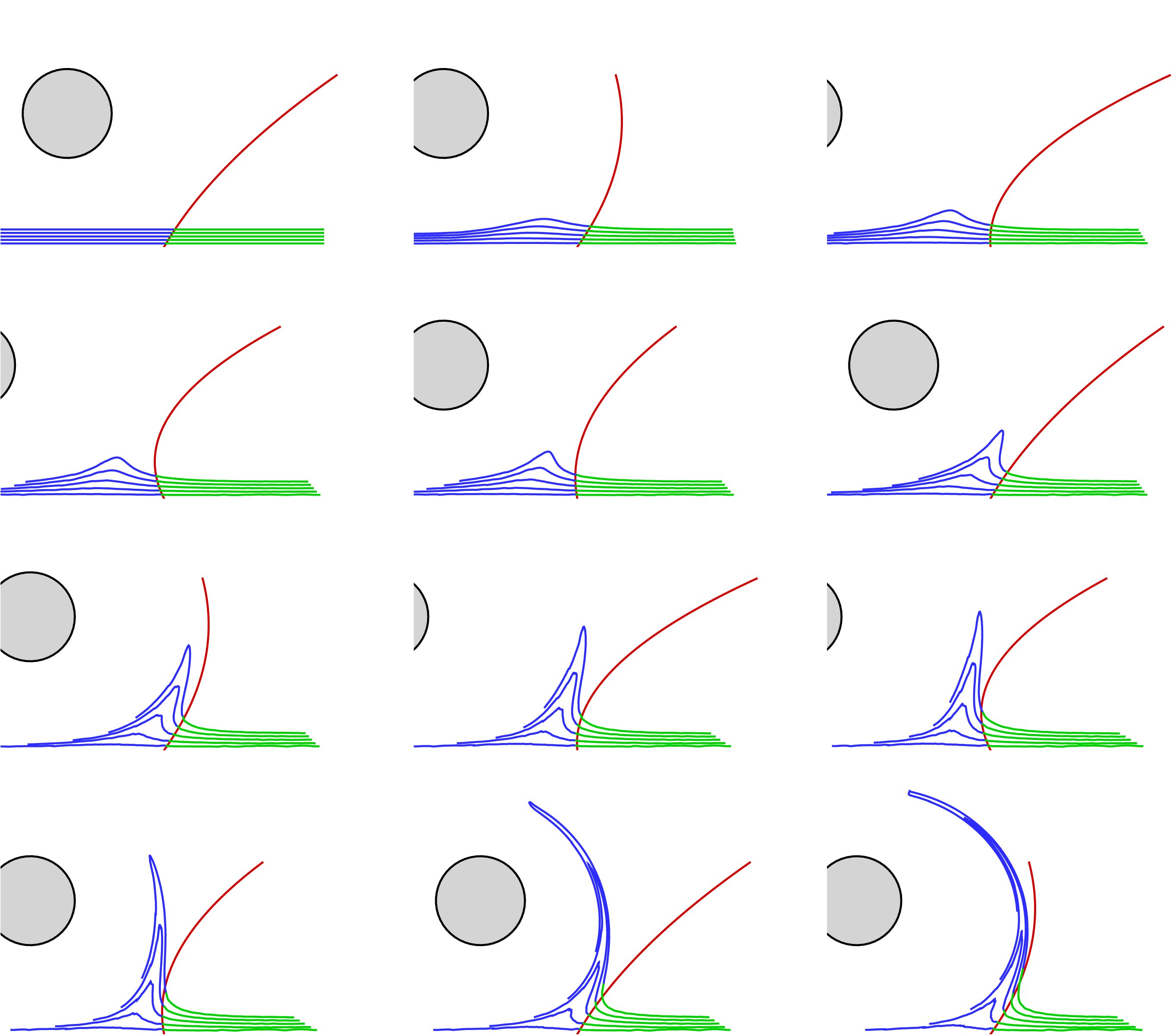
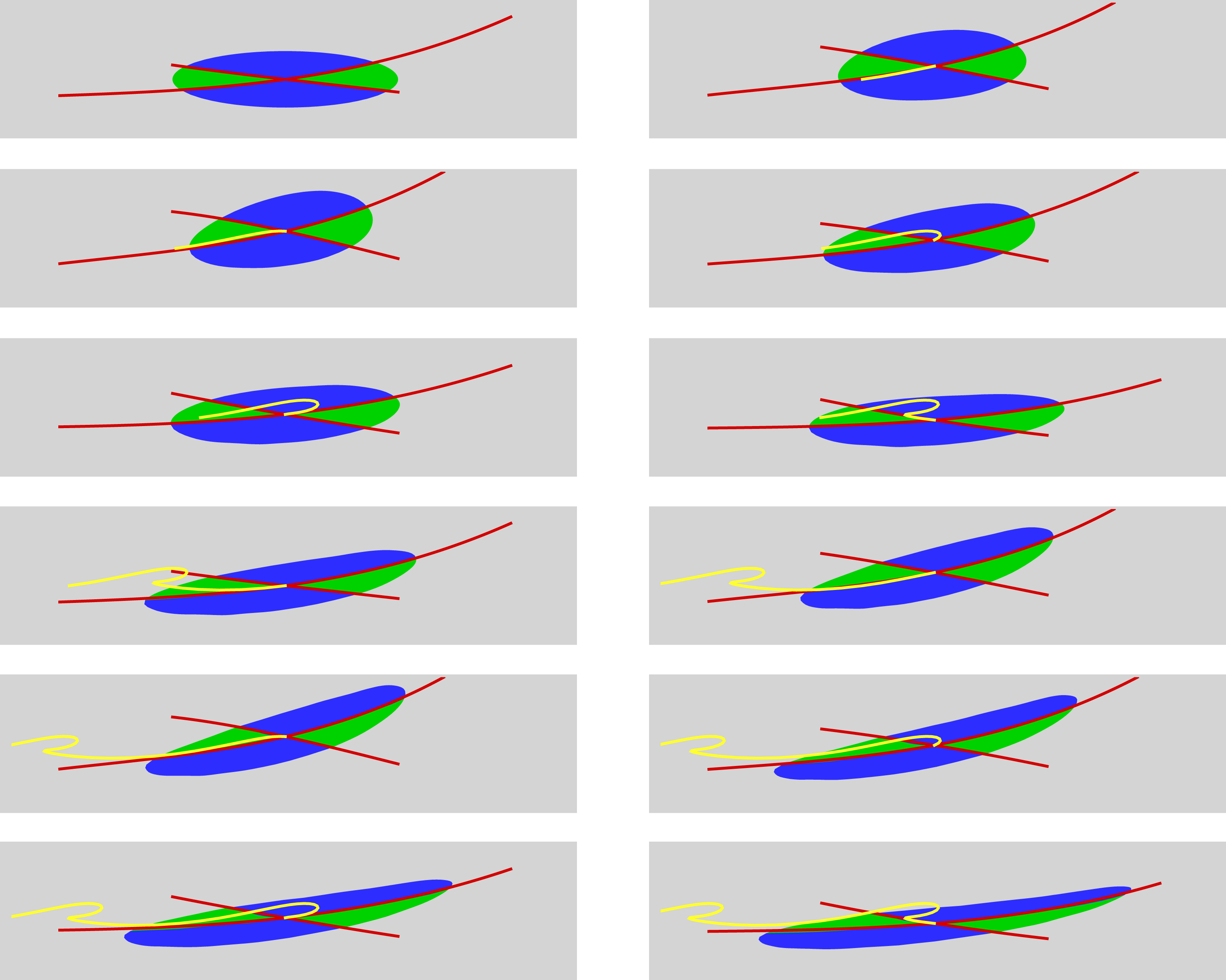
Visualisation of separation for the periodic flow (
 $\unicode[STIX]{x1D6FA}=120$
rpm,
 $\unicode[STIX]{x1D6FD}=3.8~\text{cm s}^{-1}$
and
 $f=0.4~\text{Hz}$
) with
 $H=D$
. Fluid particles are initially placed on material lines aligned with the wall using two different colours (blue and green) depending on their location in regard to the predicted separation profile (red) at the initial time
 $t=0$
. Time elapses from left to right and from top to bottom, with a time delay of
 $T/5$
(see also movie 2).

As shown in figure 3 for the four time steps presented, particle paths perfectly follow the theoretical profiles of separation. In movie 1, this is confirmed as the separation profile moves in phase with the flow, at least in the vicinity of the wall, since the profile is of second order. For a more severe case, where the distance from the wall was halved (
 $H=D$
) and the rotating velocity was doubled (
 $\unicode[STIX]{x1D6FA}=120$
rpm), phase-averaged particle images were ineffective to visualise the separation from raw PIV images. The reason is that, for these flow conditions, particles are more rapidly ejected from the wall so that over one time period, displacements of particles were too important to obtain uninterrupted material lines.
We may further note that the time-dependent separation profile prediction agrees with the particle motion close to the wall. As the distance from the wall increases, the prediction degrades but we must note that the theory provides the separation profile in terms of an approximation obtained from a series expansion in
 $y$
. Only a second-order separation profile has been computed here, and as a consequence a better agreement would have been obtained by including higher-order terms.
To overcome this difficulty, trajectories of particles, initially located on lines parallel to the wall, were computed in time using the measured velocity fields. Figure 4 presents the particles coloured differently depending on their position regarding the separation profile (in red). When advected in time, one can note that the separation profile experiences phases of positive and negative slopes, contrary to the case of figure 3, which also exposes deep curvature phases. It is however observed that it follows remarkably well the trajectory of particles in its vicinity, as blue or green tracers do not cross the separation profile, at least in the close proximity of the wall. As the distance from the wall increases, the prediction deteriorates. Indeed, fluid particles should not cross the separation profile since it is a material line (unstable manifold), but one has to note that the theory provides its instantaneous shape in terms of an approximation obtained from a series expansion in
 $y$
. Only a second-order separation profile has been computed here. A better agreement could be obtained by including higher-order terms, but this requires high-order spatial derivatives which are challenging to estimate from experimental data. Thus, depending on the geometric complexity of the true separation profile, the flow region where the predicted separation is valid may depend on time, as seems to indicate figure 4.
Two interesting and key features of the separation process are also illustrated. The first one is that while a material spike forms upstream the separation point, particles are clearly attracted by the separation profile that is represented by an unstable manifold. Thus, the theory does not predict where the spike will form, but provides elements to capture the exceptional material line that separates two flow regions with different kinematics, which is the second key feature.
4 Moving separation
If the flow is no longer periodic (
 $U_{0}\neq 0$
), a time average cannot be defined and the separation is said to be moving. While in Haller (Reference Haller2004) and Surana & Haller (Reference Surana and Haller2008) the separation point is defined at a boundary point, in Miron & Vétel (Reference Miron and Vétel2015), it is captured inside the flow off the wall, which can be represented by a Lagrangian saddle point. This is illustrated in figure 5 for the simple case where the cylinder moves with a constant speed (
 $\unicode[STIX]{x1D6FD}=0$
in (2.1)). In this case, since the flow is steady in the frame of reference moving with the cylinder, it is reasonable to think that the separation profile is also steady in this reference frame, and moves at the speed of the cylinder. To visualise it, raw PIV images were shifted following the cylinder and then averaged in time. Particle trajectories are indeed clearly apparent in figure 5, their shape marking the presence of the saddle point of separation, which also suggests that in moving separation, it is necessary to define two separation profiles instead of one. It seems however that such a separation phenomenon does not leave any signature on the wall, which prevents the use of wall-based quantities to predict it. This is because below the attracting and repelling lines, particle are first ejected from, then pushed back towards the wall, thus forming a small layer of fluid that will not separate from the wall. In the more general case with arbitrary time dependence, the prediction of separation requires first to capture the saddle point. The next section provides a method to extract such separation when the cylinder moves as per (2.1).
Visualisation of separation for the translating cylinder (
 $\unicode[STIX]{x1D6FA}=60$
rpm,
 $U_{c}=1~\text{cm s}^{-1}$
) with
 $H=2D$
. Particle images were first shifted following the cylinder displacement, then averaged over a long period of time to maintain the observer in a frame of reference moving with the cylinder. The cylinder moves from left to right.

4.1 Detection method
For the general cylinder motion (2.1) with
 $U_{0}\neq 0$
, the flow is periodic in a frame of reference moving with the cylinder, i.e. the flow pattern, seen from the cylinder, is the same for time instants
 $t_{n}=t_{0}+nT$
, where
 $n$
is an integer. Therefore, it is supposed that the separation point and profiles are material quantities with fixed locations relative to the cylinder for multiples of the time period.
In this case, an alternative method to the one adopted in Miron & Vétel (Reference Miron and Vétel2015) can be used to capture the separation geometry, which does not require the extraction of Lagrangian coherent structures (LCS) that can be more sensitive to noise. At time
 $t_{0}$
, the saddle point of separation is first extracted by seeking a point
 $\boldsymbol{x}_{s}=(x_{s}(t),y_{s}(t))$
such that
 $$\begin{eqnarray}\Vert \boldsymbol{x}_{s}(t_{0}+T)-\boldsymbol{x}_{s}(t_{0})-U_{0}T\Vert ^{2}=0.\end{eqnarray}$$
Then, in a manner similar to the method developed by Haller (Reference Haller2004), the two separation profiles, defining the flow behaviour in the vicinity of the Lagrangian saddle point, are described by the following equation
 $$\begin{eqnarray}y=y_{s}+(x-x_{s})F(x-x_{s},t),\end{eqnarray}$$
where
 $F$
is a series expansion in the form
 $$\begin{eqnarray}F(z,t)=f_{0}(t)+zf_{1}(t)+{\textstyle \frac{1}{2}}z^{2}f_{2}(t)+\cdots \,.\end{eqnarray}$$
By differentiating (4.2) with respect to time, we obtain the expression
 $$\begin{eqnarray}v=v_{s}+(u-u_{s})F+(x-x_{s}){\dot{F}},\end{eqnarray}$$
where all quantities are Lagrangian, i.e. are calculated following the trajectory of the particle that is chosen at the initial time
 $t_{0}$
.
Each
 $f_{k}$
coefficient can then be computed by successively differentiating equation (4.4) with respect to
 $x$
and setting
 $\boldsymbol{x}=\boldsymbol{x}_{s}$
. For example, the following expression is obtained for the angle
 $f_{0}$
of any material line passing through
 $\boldsymbol{x}_{s}$
:
 $$\begin{eqnarray}\dot{f_{0}}=v_{x}+(v_{y}-u_{x})f_{0}-u_{y}f_{0}^{2},\end{eqnarray}$$
where spatial derivatives of the velocity components are defined on the trajectory of the separation point. Equation (4.5) was numerically integrated and solved for
 $f_{0}(t_{0})$
for which
 $$\begin{eqnarray}f_{0}(t_{0}+T)=f_{0}(t_{0}),\end{eqnarray}$$
which yields to the determination of two solutions, corresponding to the repelling and attracting lines defining the separation process.
Expression of higher-order terms
 $f_{k}$
for
 $k\geqslant 1$
can then be explicitly obtained. In incompressible flows, by differentiating (4.4) twice with respect to
 $x$
, the differential equation for
 $f_{1}$
takes the form
 $$\begin{eqnarray}\dot{f_{1}}+gf_{1}=h,\end{eqnarray}$$
with
 $$\begin{eqnarray}\left.\begin{array}{@{}c@{}}\displaystyle g=3(u_{x}+f_{0}u_{y});\\ \displaystyle h={\textstyle \frac{1}{2}}[v_{xx}-3f_{0}u_{xx}-3f_{0}^{2}u_{xy}-f_{0}^{3}u_{yy}].\end{array}\right\}\end{eqnarray}$$
By posing
 $$\begin{eqnarray}\unicode[STIX]{x1D70C}(t)=\exp \left(-\int _{t_{0}}^{t}g(\unicode[STIX]{x1D70F})\,\text{d}\unicode[STIX]{x1D70F}\right),\end{eqnarray}$$
the general solution of (4.7) is
 $$\begin{eqnarray}f_{1}(t)=\unicode[STIX]{x1D70C}(t)\left[f_{1}(t_{0})+\int _{t_{0}}^{t}\frac{h(\unicode[STIX]{x1D70F})}{g(\unicode[STIX]{x1D70F})}\,\text{d}\unicode[STIX]{x1D70F}\right].\end{eqnarray}$$
Again, the shape of the separation is periodic in time so that
 $f_{1}(t_{0}+T)=f_{1}(t_{0})$
, which, with (4.10), gives
 $$\begin{eqnarray}f_{1}(t_{0})=\frac{\unicode[STIX]{x1D70C}(t_{0}+T)}{1-\unicode[STIX]{x1D70C}(t_{0}+T)}\int _{t_{0}}^{t_{0}+T}\frac{h(\unicode[STIX]{x1D70F})}{g(\unicode[STIX]{x1D70F})}\,\text{d}\unicode[STIX]{x1D70F}.\end{eqnarray}$$
Similar expressions to (4.11) can also be derived for all other coefficients but will not be presented for simplicity.
4.2 Results
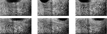
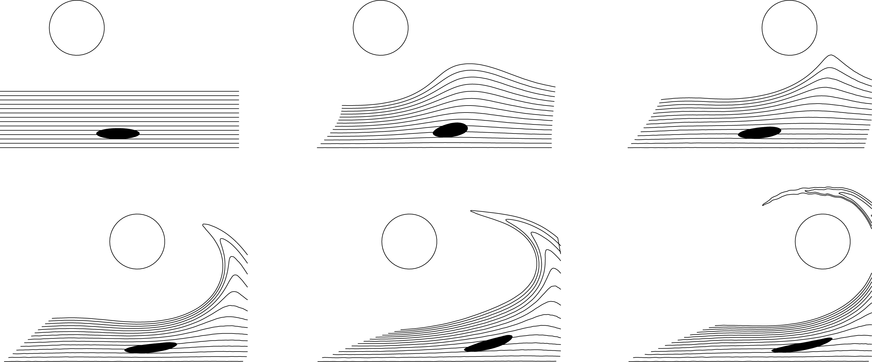
To first visualise separation on raw images, figure 6 shows one period of oscillation for a moderate oscillation with
 $\unicode[STIX]{x1D6FD}=2U_{0}$
. Five consecutive images were averaged while following the separation point obtained by solving (4.1), then the two separation angles were deduced with (4.6) and finally the
 $f_{k}$
coefficients were deduced recursively from expressions similar to (4.11) up to third order. The resulting two material lines are superposed in yellow on figure 6. It is shown that as expected, particle paths around the separation point tend to align with the four branches forming the saddle point (top images). An interesting feature is that the separation point does not follow the cylinder motion but is on the contrary out of phase with it. However, in the bottom images, the agreement seems less obvious.
Visualisation of separation for the translating and oscillating cylinder (
 $\unicode[STIX]{x1D6FA}=60$
rpm,
 $U_{0}=1~\text{cm s}^{-1}$
,
 $\unicode[STIX]{x1D6FD}=2~\text{cm s}^{-1}$
and
 $f=0.5~\text{Hz}$
) with
 $H=2D$
. Particle images were averaged over five consecutive images (0.3 s) centred on each time step in a frame of reference moving with the separation point defined by a Lagrangian saddle point. Time elapses from left to right and from top to bottom, with a time delay of
 $T/6$
.

Same as in figure 6 but with
 $\unicode[STIX]{x1D6FD}=8~\text{cm s}^{-1}$
.

Further investigations were carried out by using a more severe cylinder movement. Figure 7 presents for example the same image treatment as in figure 6 but with
 $\unicode[STIX]{x1D6FD}=8U_{0}$
(separation profiles not shown). While the presence of a saddle point is observed in the first two images as well as in the last one, other images rather exhibit the presence of recirculation regions which does not seem to indicate the presence of a saddle point. However, this visualisation remains qualitative, and furthermore does not indicate flow direction.
Prediction of moving separation for the same flow parameters as in figure 7. Particles (seen in a reference frame moving with the separation point) are released with a colour (blue or green) depending on their initial location relative to the red lines that correspond to the predicted attractive and repulsive lines that define the separation point which moves on the yellow trajectory. Time elapses from left to right and from top to bottom, with a time delay of
 $T/6$
(see also movie 3).

To best visualise the flow organisation between the cylinder and the wall, figure 8 presents more precisely the trajectories of fluid particles initially released inside an ellipse with a colour depending on their position relative to the separation profiles. The particles were then advected in time through the velocity field time series, with the computed separation lines (in red) superimposed for several time instants. The observer is linked to the reference frame moving with the separation point whose trajectory appears in yellow. One can observe that the particles perfectly follow the predicted separation profiles during the two periods shown.
It is important to note that the ellipse stretch direction is not necessarily aligned with the attracting material line, and that the compression direction does not coincide with the repelling line. Indeed, as in the case of the purely oscillating flow (cf. figure 4), the separation profiles allow us to detect material barriers in the frontiers of dynamically different flow regions. Here, this illustrates that particles in blue are either attracted by or ejected from the wall, but that particles in green will never reach the wall, at least on a short time horizon. A more general view of flow separation is also presented in figure 9 by advection of particles initially aligned with the wall.


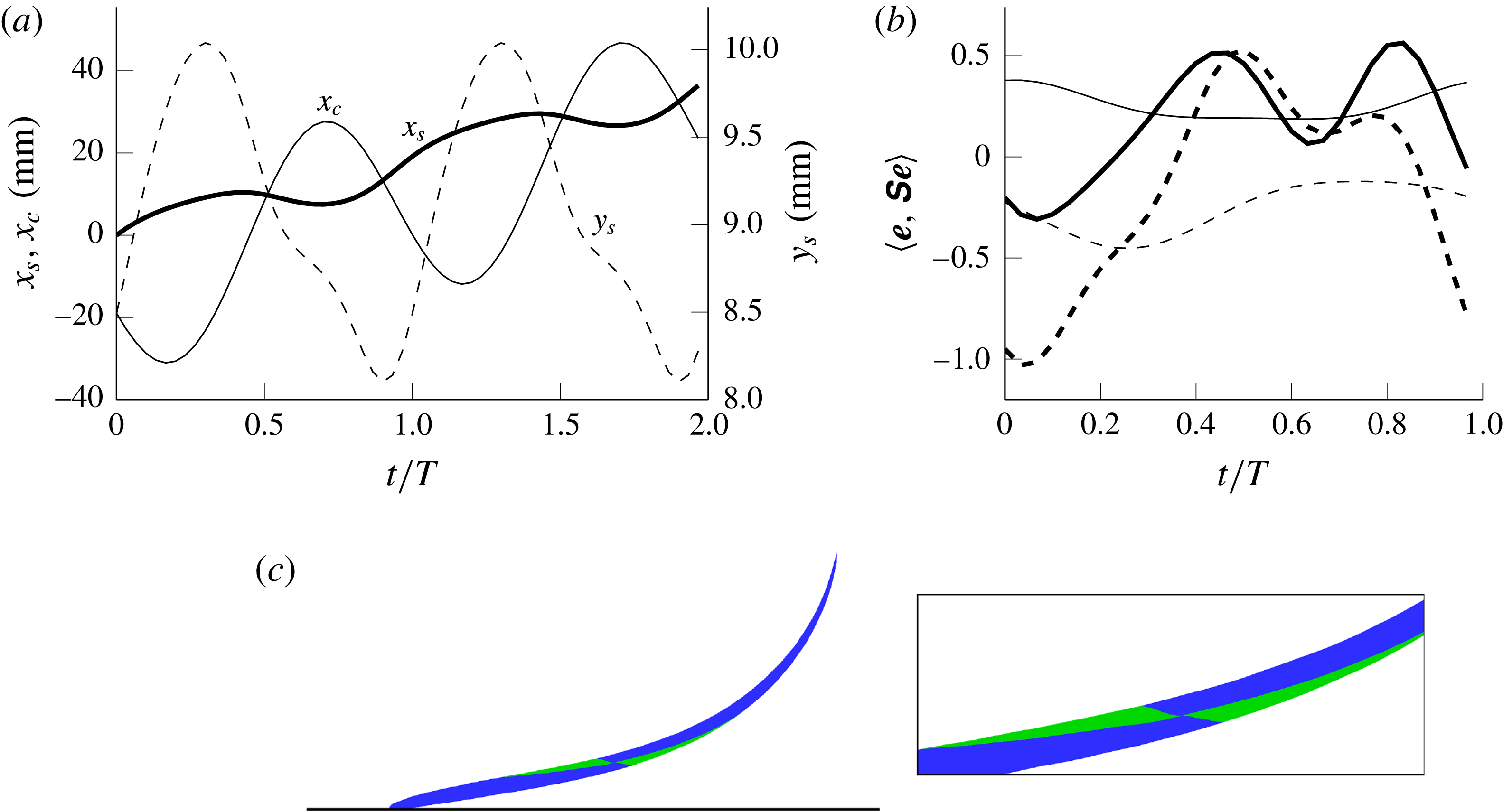
(a) Trajectory of the separation point
 $(x_{s},y_{s})$
compared with that of the cylinder
 $(x_{c})$
for the same flow parameters as in figure 7 over two time periods. (b) Evolution of the tangential rate of strain
 $\langle \boldsymbol{e},\unicode[STIX]{x1D64E}\boldsymbol{e}\rangle$
for the attracting material line (solid lines) and the repelling material line (dashed lines) for the case in (a) (thick lines) and the less severe conditions of figure 6 (thin lines). In (c), a visualisation of the deforming flow pattern around the separation point for these less severe conditions is provided at
 $t=2T$
for initial positions contained inside a circle centred on the separation point and tangent to the wall (data used in figure 6).

To provide more insights into the separation process, figure 10(a) compares the horizontal trajectory of the separation point
 $x_{s}$
to that of the cylinder
 $x_{c}$
for the case of figure 8. It is confirmed that both amplitude and phase are different, indicating that the separation point is not fixed relative to the cylinder. Moreover, while the vertical position of the cylinder is fixed, that of the separation point
 $y_{s}$
is moving. It is indeed observed that the trajectory of a Lagrangian separation point does not generally follow the unsteadiness of the Eulerian flow (Miron, Vétel & Garon Reference Miron, Vétel and Garon2015; Miron & Vétel Reference Miron and Vétel2015). This reflects for a moving separation what has already been observed for a fixed separation. Indeed, in a periodic flow, as presented in § 3, the separation point does not follow the cylinder as it is in reality fixed to the wall. On the contrary, the point where the shear stress vanishes on the wall can oscillate in space on a large extent, and thus the true separation point does not reflect this temporal time scale (Haller Reference Haller2004), illustrating again that the Prandtl criterion is not valid in unsteady flows.
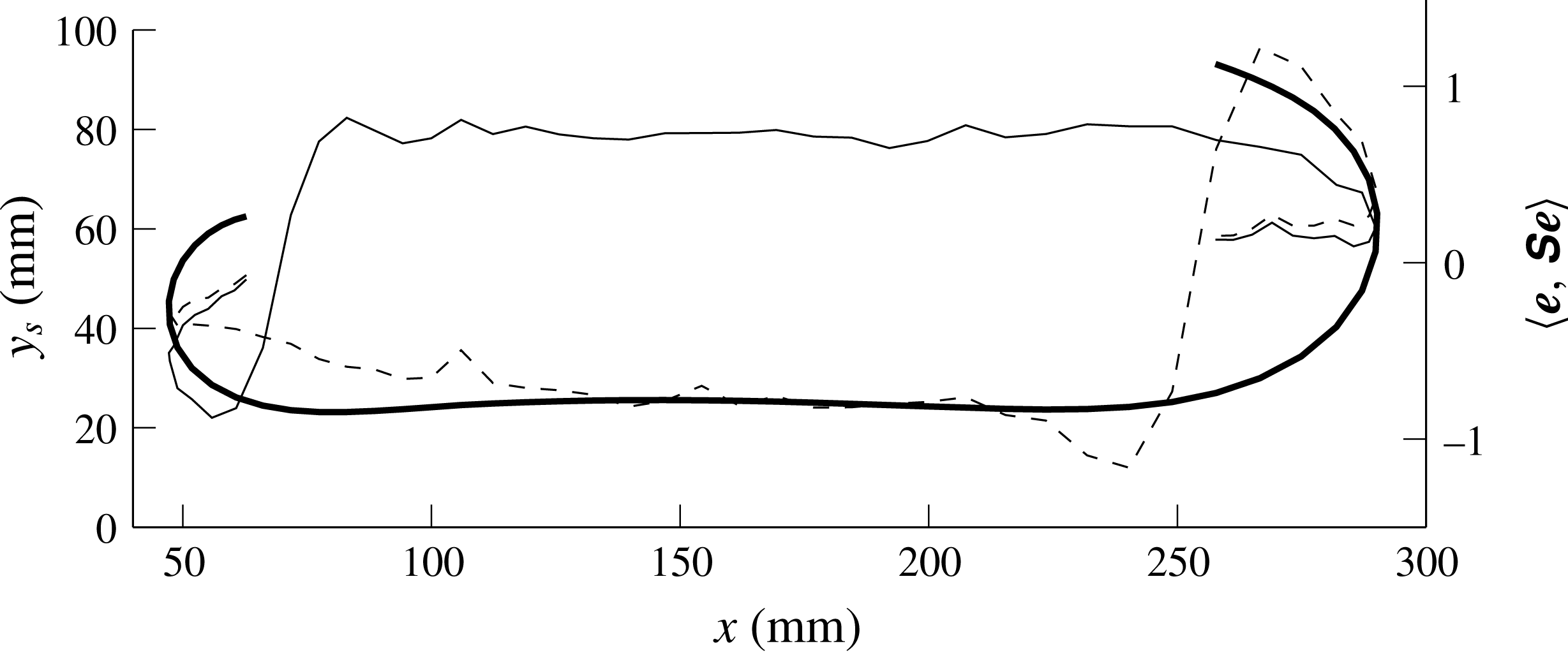
An examination of the rate of strain along the two separation profiles is plotted in figure 10(b) over one time period, with the case of figure 10(a) in thick lines. The solid line, relative to the attractive material barrier, shows that
 $\langle \boldsymbol{e},\unicode[STIX]{x1D64E}\boldsymbol{e}\rangle$
is positive for
 $t/T\geqslant 0.25$
, while for the repelling line,
 $\langle \boldsymbol{e},\unicode[STIX]{x1D64E}\boldsymbol{e}\rangle$
is negative for
 $t/T\in [0;0.35]\cup [0.85;1]$
, which confirms the fact that the separation profiles are not necessarily aligned with the most stretching and compression strain rate directions (which are orthogonal in incompressible flows). On the contrary, the same results, examined for the less severe case of figure 6, and plotted on figure 10 with thin lines, show that
 $\langle \boldsymbol{e},\unicode[STIX]{x1D64E}\boldsymbol{e}\rangle$
remains positive (respectively negative) at the separation location on the attracting (respectively repelling) line during the whole period, which indicates the saddle-type behaviour of the separation point. However, in (c) are shown the locations of particles in a manner similar to what was presented in figure 8 but for the flow conditions of figure 6 after two period of motion. Here, instead of using an ellipse, particles were released from a circle centred on the separation point and reaching the wall. It is again interesting to see that particles in green have a slow evolution compared to other particles in blue and that this dynamics is well captured by the separation profiles, which do not align with the most stretching and compression rate directions.
5 Intermediate cases
In this section two cases will be explored, the first one when the period of oscillation is increased, which results in a long translation movement of the cylinder, and a second one where the cylinder velocity is gradually decreased to zero.
5.1 Slow oscillatory motion
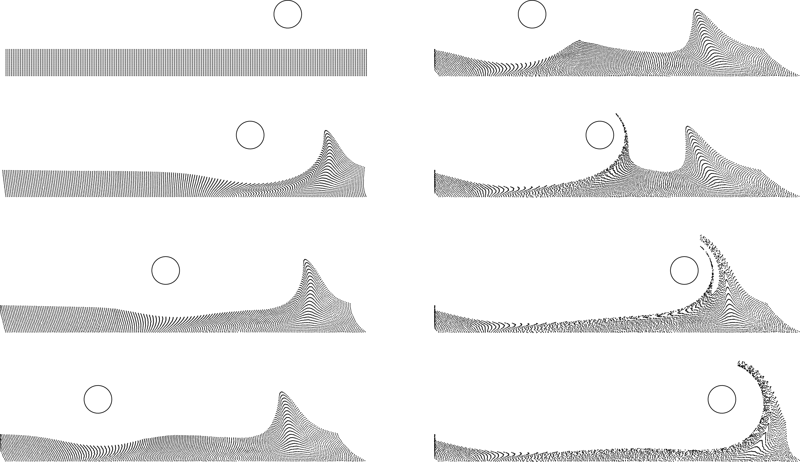
Results for the first case are presented in figures 11–13. For this case, the flow is periodic with a frequency as low as
 $f=0.05~\text{Hz}$
, so that the peak-to-peak amplitude of the cylinder motion reaches
 ${\sim}18~\text{cm}$
while positioned at
 $2D$
form the wall. Two PIV cameras where used side by side to obtain a large field of view. In figure 11, the cylinder motion is visualised on a whole period, together with tracer particles initially located below
 $y=D$
on the whole length of the measurement area. Since the flow is periodic, the theory of Haller (Reference Haller2004) predicts the presence of a fixed separation point at the wall. This is indeed the case when the cylinder moves to the left (left panels). However, on the way back (right panels), an additional separation moving with the cylinder is also simultaneously observed. As expected, the time scale of the translational motion being longer than that of the rotation of the cylinder, fluid particles are extracted from the wall. It is interesting to see that while for the moving case a large amount of particles stays in the vicinity of the wall, with subsequent passages of the cylinder, they are gradually displaced towards the fixed separation point where they will finally be ejected from the wall.
Ejection of particles initially located in the vicinity of the wall for the case of the periodic flow with a long period (
 $\unicode[STIX]{x1D6FA}=60$
rpm,
 $\unicode[STIX]{x1D6FD}=2.9~\text{cm s}^{-1}$
,
 $f=0.05~\text{Hz}$
and
 $H=2D$
). Time elapses from top to bottom and from left to right, with a time delay of
 $T/7$
(see also movie 4).

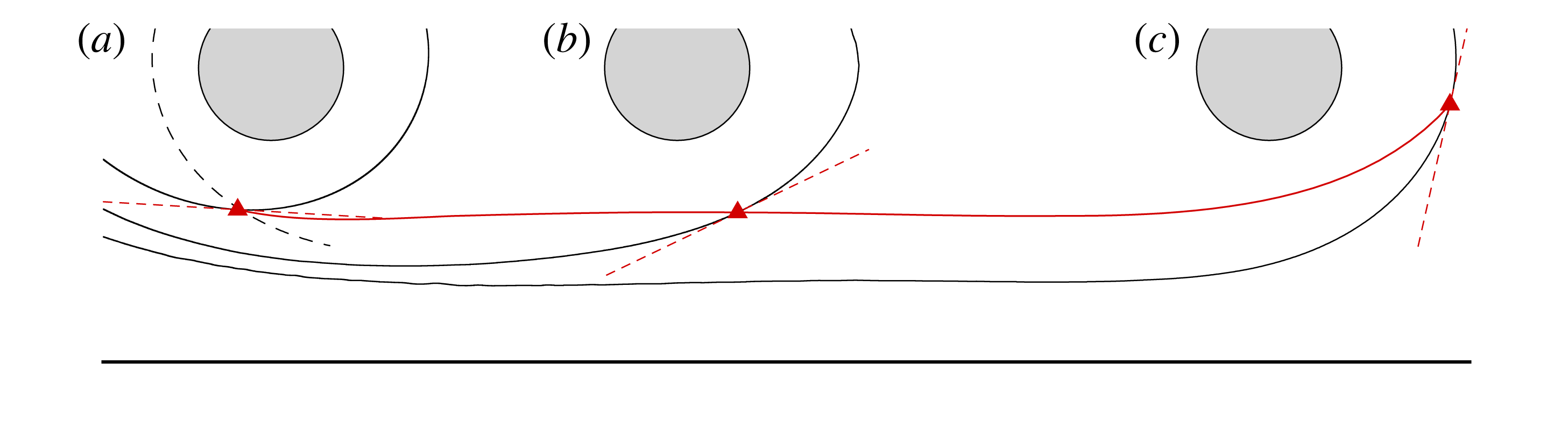
Trajectory of the separation point (solid red line) for the same conditions as in figure 11. The initial position
 $t=0$
in (a) is indicated by the red triangle, defined as the intersection point between the attracting LCS (solid black line) and the repelling LCS (dashed black line). The location of the separation point, together with the attracting LCS and the separation slope (dashed red line), is followed in (b) at
 $t=T/7$
and in (c) at
 $t=T/3$
.

The moving separation point can no longer be captured by the method used in § 4.1 because, considering the large time period, it is ejected from the wall and its trajectory can no longer be captured by the PIV technique. To detect it, LCSs were first extracted using the method described in Haller (Reference Haller2011) and Farazmand & Haller (Reference Farazmand and Haller2012). In figure 12(a), the solid black line represents the most attracting LCS in the flow (obtained in backward time) while the dashed line is the most repelling one (obtained in forward time), the intersect of which defines a hyperbolic point corresponding to the separation point. The attracting LCS was then advected in time together with the separation point and the slope of the separation profile deduced from Miron & Vétel (Reference Miron and Vétel2015). This is shown in figure 12(b) for
 $t=T/7$
and in (c) for
 $t=T/3$
. As observed, the trajectory of the separation point (solid red line) is almost horizontal, similar to the case when the cylinder is moving with a pure translational velocity. The LCS also tends to align parallel to the wall, thus delimiting a material barrier below which particles are not extracted from the wall. In figure 12(c), however, the separation point is in turn ejected in the flow.
Evolution of the tangential rate of strain
 $\langle \boldsymbol{e},\unicode[STIX]{x1D64E}\boldsymbol{e}\rangle$
for the attracting material line (thin solid line) and the repelling material line (dashed line) for the same conditions as in figures 11 and 12 when the cylinder moves from left to right. The trajectory
 $y_{s}$
of the separation point is indicated by the thick solid line.

A more complete trajectory of the separation point is shown in figure 13, as well as the time history, along this trajectory, of the tangential rate of strain on the attracting and repelling LCS initially located in figure 12(a). One may observe that the separation point appears as a saddle-type point when
 $\langle \boldsymbol{e},\unicode[STIX]{x1D64E}\boldsymbol{e}\rangle$
is simultaneously positive on the attracting LCS (solid line) and negative on the repelling LCS (dashed line), which happens for
 $x\in [70~\text{mm},250~\text{mm}]$
. Again, these rates are almost constant on a large portion of the cylinder motion, despite the acceleration and deceleration phases, thus illustrating again that the Lagrangian quantities are not weakly related to the unsteadiness of the Eulerian velocity fields.
5.2 From moving to fixed separation
As a last example, we show here how a moving separation becomes a fixed one. To this end, the cylinder, moving initially at a constant velocity, is then decelerated down to a fixed position to observe the transition. In the context of the theory of Haller (Reference Haller2004), the separation in this case is moving. Since classical invariant manifold theory cannot apply, Haller (Reference Haller2004) used finite-time unstable manifolds (Haller Reference Haller2000) to capture the moving point, but yielded to non-unique moving separation profiles. Alternatively, Surana & Haller (Reference Surana and Haller2008) proposed to define the location of the moving separation point where the time-varying mean skin friction vanishes. In the present case, where flow fluctuations are absent, separation is predicted to appear at the instantaneous zero skin-friction point, but this was not observed.
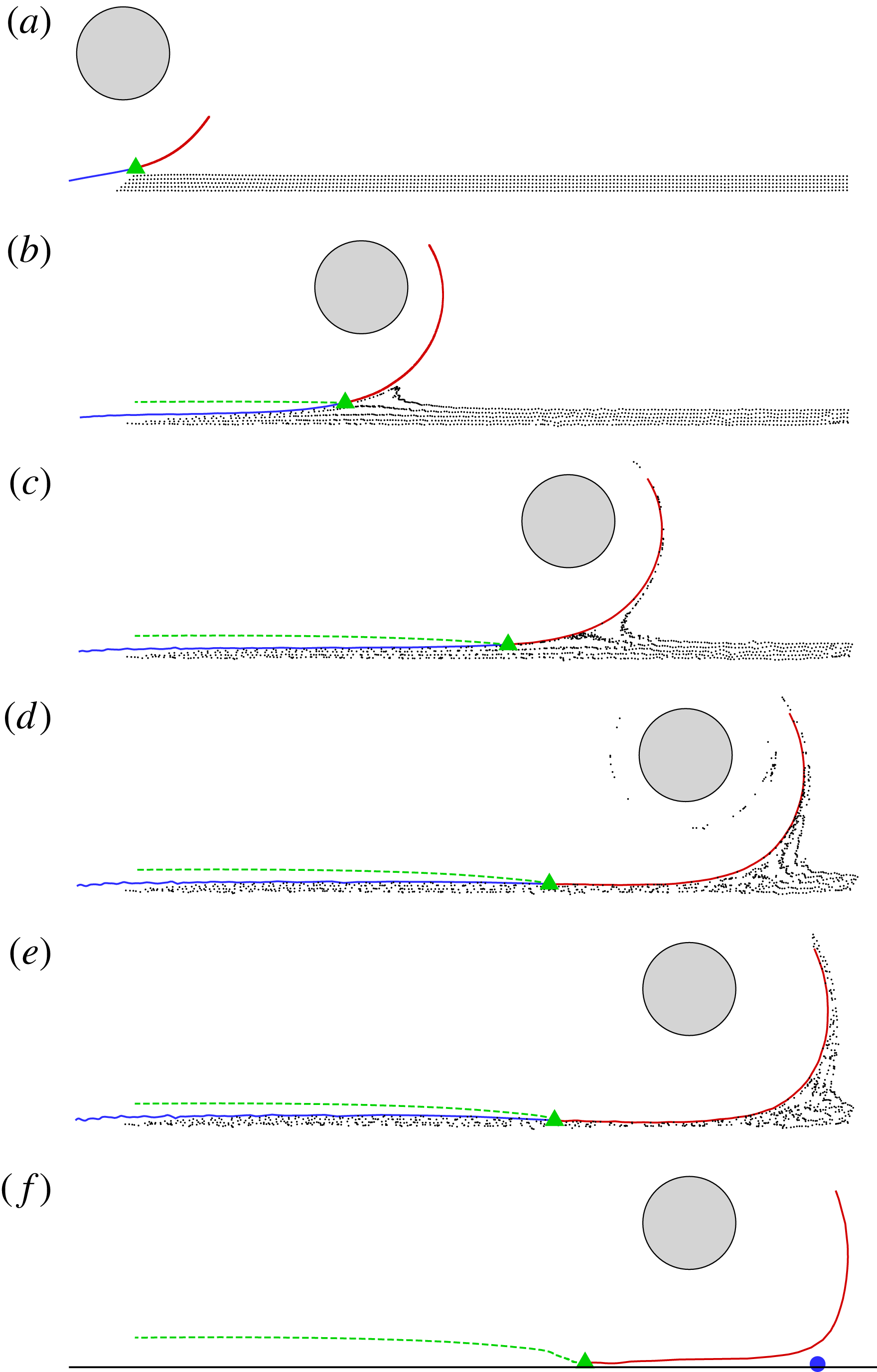
Visualisation of separation for a cylinder decelerating from a constant velocity to zero following a hyperbolic tangent velocity profile. The moving separation point (green triangle) was captured during the phase of constant velocity and was then tracked until the cylinder stops moving, together with its associated attracting material line (red and blue). Time elapses from top to bottom with a constant time delay for plots (a–e). In (f), visualisation of the upper part of the attracting material line is shown a long time after the cylinder has stopped, the blue point indicating the location where the wall shear stress vanishes.

Results on moving separation are summarised in figure 14. In figure 14(a), the separation profile (attracting line) was obtained in a similar manner as in § 4.1 but simpler as here the separation geometry translates at the cylinder velocity, i.e. the separation profiles are steady in a reference frame co-moving with the cylinder. After this phase, the cylinder is decelerated to zero following a hyperbolic tangent profile and reaches its final position at the instant shown in figure 14(d). During the whole movement, the separation point and profile identified in figure 14(a) were also advected in time from figure 14(a) to figure 14(e). A smooth transition from moving to fixed separation is therefore completely captured. In particular, we observe that the moving separation point in the first flow phase is slowly abandoned by the separation process during the declaration phase. After a sufficient long time, the flow becomes steady with a point of vanishing wall shear stress indicated by the blue point in figure 14(f). Therefore, this example illustrates the complexity to capture adequately the separation point in an unsteady flow with arbitrary time dependence. It reveals that for a general theory able to detect complex separation phenomena, a criterion must be constructed on short time intervals, as the time dependence may imply different separation points existing simultaneously inside a same flow. In the following section, we investigate a different but more practical example showing that situations examined until now throughout this paper are not unique to our particular experimental set-up.
5.3 The impinging jet
The round impinging jet has been extensively studied in the literature for several reasons. It is used in many industrial processes for cooling or heating, and in parallel, represents a pertinent test case for the validation of turbulent models. Despite the simple geometry, the flow physics is complex, which means that it is also of interest for fundamental studies. The most active research topic probably concerns the presence of a secondary maximum in the radial distribution of the mean heat transfer. Many studies have attempted to explain this particularity by attributing this effect to the unsteady separation that occurs when the jet vortices impact the plate, or to a laminar turbulent transition. However, the real origin of this was only discovered by Dairay et al. (Reference Dairay, Fortuné, Lamballais and Brizzi2015). While they indeed observe, in their DNS study, that the secondary peak is located near the separation line, they show that it is the result of azimuthal distortions of secondary vortices followed by the formation of radially elongated small scale structures. These distortions thus generate localised intense heat transfer zones similar to cold spot on the heated wall. Therefore, this effect is mainly three-dimensional, which implies that it should be very weak or completely absent in two-dimensional numerical simulations.
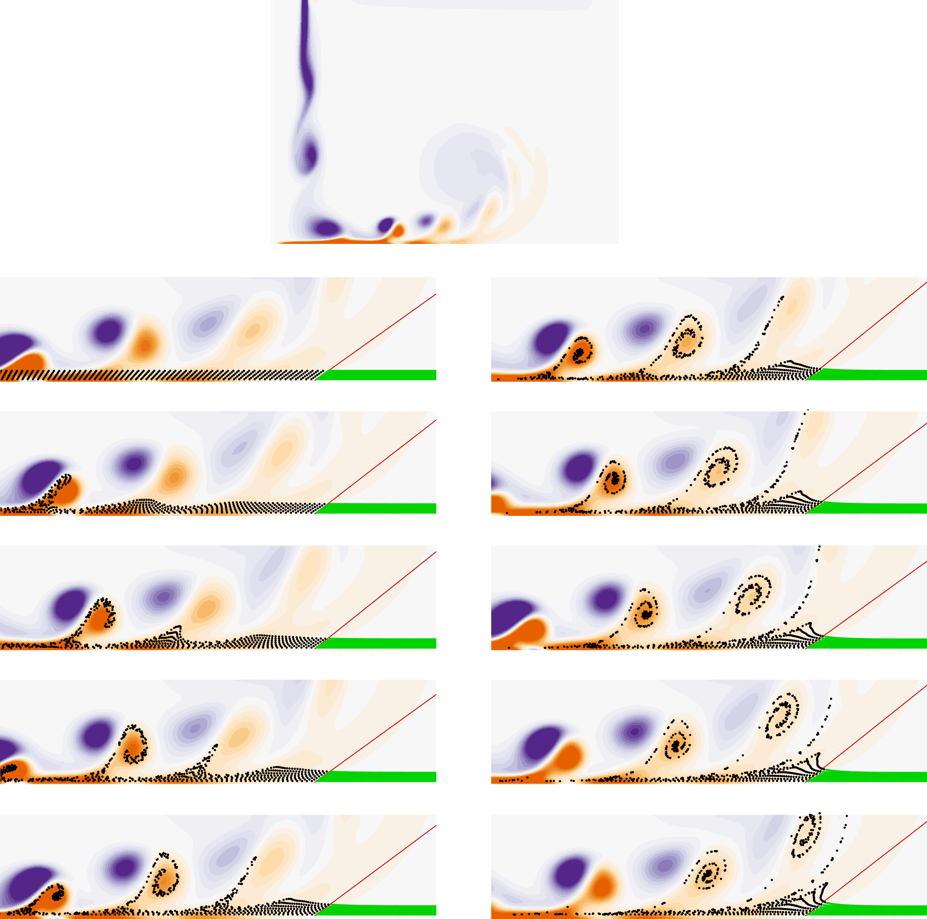
Visualisation of separation (red line) in an impinging jet with a nozzle-to-plate distance
 $H/D=4$
. The top image shows the full vorticity field while the bottom images show a zoomed view on the fixed separation revealed with fluid particles of different colours. Time elapses from top to bottom and from left to right, with a time delay of
 $0.15D/U_{jet}$
.

To investigate unsteady separation in a round impinging jet, a two-dimensional, incompressible, axisymmetric impinging jet with heat transfer has been computed with the open source finite element code FreeFem++ (Hecht Reference Hecht2012). The Reynolds number, based on the jet diameter
 $D$
and the jet velocity
 $U_{jet}$
is
 $Re=1000$
. As boundary conditions, a hyperbolic tangent velocity profile is prescribed for the jet exit velocity, and a no-slip velocity at the wall surrounding the jet exit. The temperature at the jet exit boundary is constant at
 $T=T_{jet}$
and a constant flux
 $\unicode[STIX]{x1D711}$
is prescribed on the impingement wall.
Two nozzle-to-plate distances
 $H/D$
have been considered. Figure 15 presents the vorticity contours (top image) obtained with
 $H/D=4$
. The left boundary of the field of view coincides with the symmetry axis of the jet that is orientated to the bottom. The primary vortices issued from the jet instability are marked by counter-clockwise vorticity (purple) and as they impact on the wall, they generate secondary clockwise vortices (orange). This is accompanied by an unsteady separation that moves with the primary vortices (see, e.g., Didden & Ho Reference Didden and Ho1985). A close-up view of this phenomenon is also presented for several time instants in figure 15, where particles have been initially located on lines parallel to the wall and then advected in time (in black). As time elapses, we indeed clearly observe that they are gradually extracted from the wall through multiple vortex-induced separation processes (Doligalski, Smith & Walker Reference Doligalski, Smith and Walker1994; Cassel & Conlisk Reference Cassel and Conlisk2014). However, we can also note that particles closest to the wall are not ejected. For example, after the passage of the first vortex (left figures), some particles are still present in the vicinity of the boundary, but will eventually be extracted by the passage of the following vortices. This separation is a clear illustration that the separation is moving, similar to what was observed with the cylinder (cf. figure 11). This in fact corroborates the explanation provided by Dairay et al. (Reference Dairay, Fortuné, Lamballais and Brizzi2015) who attributed the local cooling effect by a three-dimensional vortex organisation, but not to unsteady separation. As we see here, after the passage of a vortex, a fluid layer is still confined on the wall thus inhibiting the heat transfer.
In the results of figure 15, the flow is periodic. According to Haller (Reference Haller2004), a fixed separation should be observed where the wall shear stress, averaged over one period, vanishes. Formulae detailed in Haller (Reference Haller2004) have then been applied to compute the location of separation and the unsteady slope of the separation profile. This is shown in figure 15 by the red line, and the same particles that were used to visualise the unsteady separation are also used here with a different colour (green) downstream of the theoretical separation profile. It is remarkable to see that the theory is still valid in this flow since the separation profile indeed marks a clear material boundary between the upstream flow that is ejected from the wall and the downstream flow that remains in its vicinity. We can also note that a material spike forms upstream of the fixed separation point. This is therefore very similar to the case of the cylinder oscillating with a long period described in § 5.1 where both separation types were simultaneously present (cf. figure 11), the cylinder rotation being here replaced by a vortex. However, for the jet, the downstream flow is only weakly unsteady; we nonetheless observe an oscillation of the instantaneous vanishing wall shear stress location (not shown), thus invalidating the Prandtl criterion for this flow.
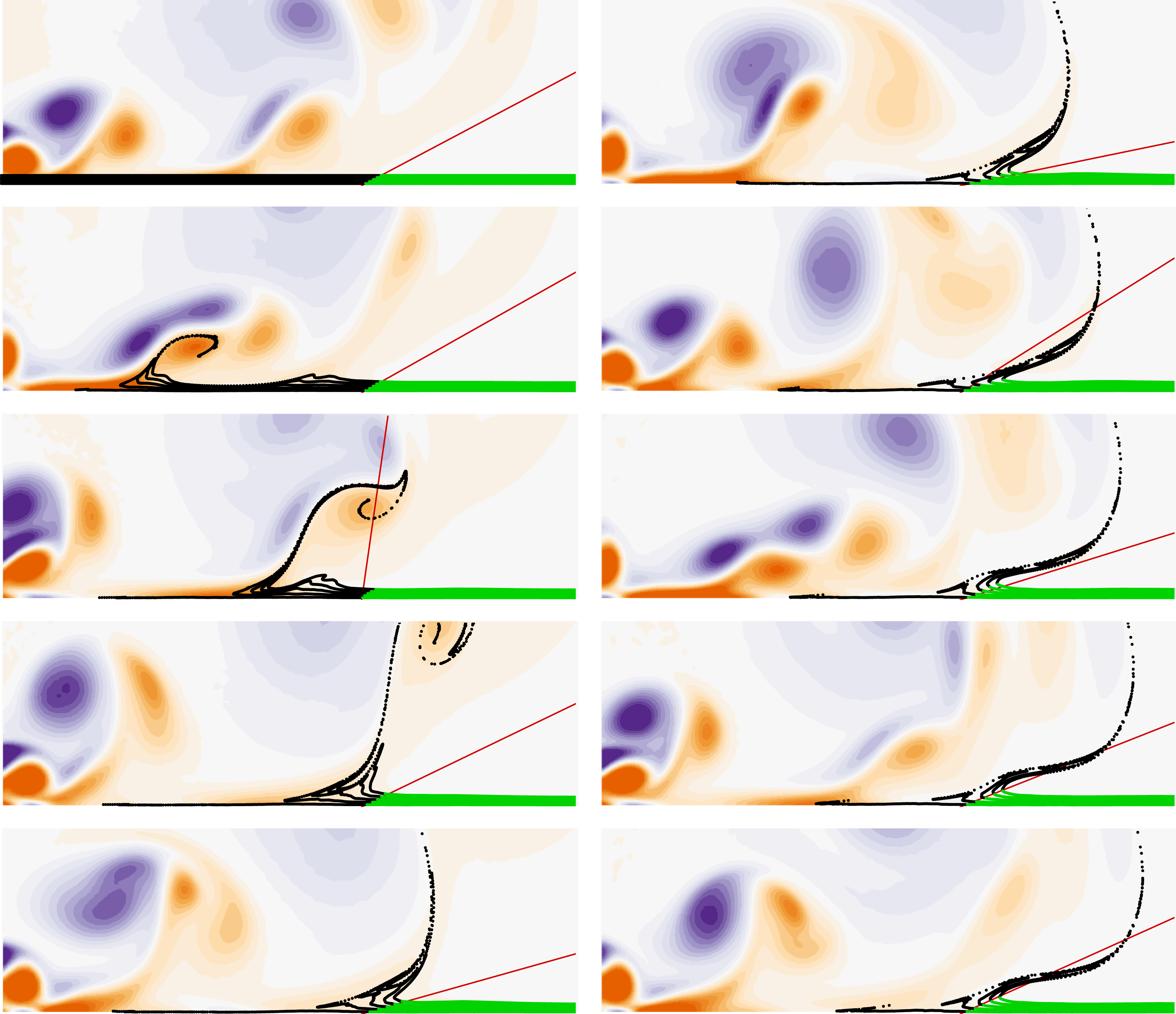
Same as in figure 15 but with a nozzle-to-plate distance
 $H/D=2$
and a time delay of
 $0.1D/U_{jet}$
.

To complete these observations, figure 16 shows the same visualisations but for
 $H/D=2$
. For this configuration however, the periodicity of the previous case was not observed. Yet, as a time-mean flow can be obtained, a fixed separation is also predicted by the theory. Formulae relative to non-periodic situations given in Haller (Reference Haller2004) have been applied and results are presented in figure 16 similarly as in figure 15. Vorticity contours reveal that intermittent vortex pairings occur at different locations in the flow, thus removing any periodicity in the flow. Nevertheless, it is remarkable to observe that a fixed separation is still defined and that the unsteady slope is well predicted by the theory. Again, particle upstream the fixed separation point are rapidly ejected inside the flow whereas ones downstream stay close to the wall, even at large time instants.


Between the case
 $H/D=4$
of figure 15 and the case
 $H/D=2$
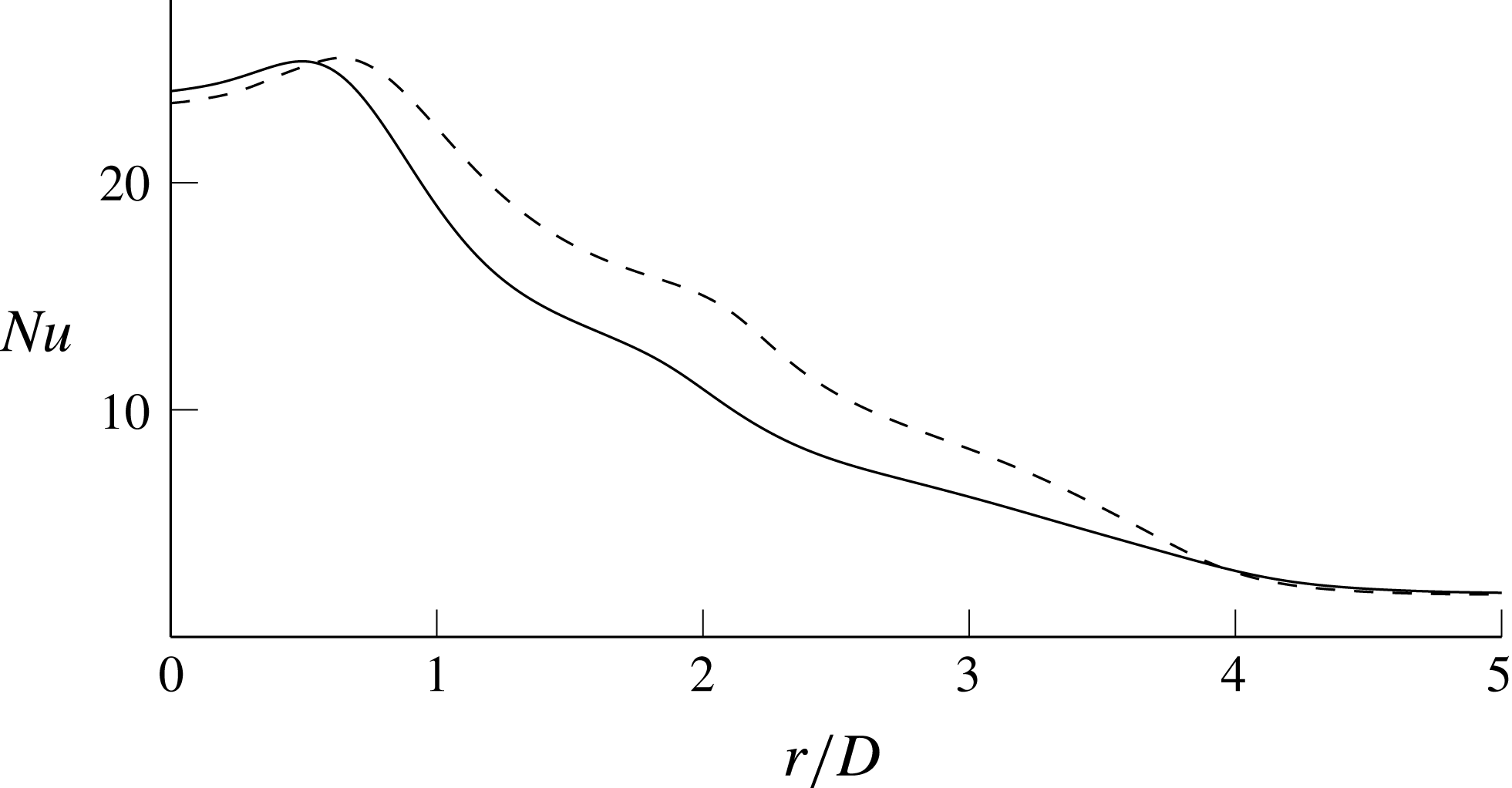
of figure 16, one can remark that particles close to the wall in the upstream area of the flow are rapidly ejected for the latter in comparison to the former. To investigate this effect on the heat transfer, figure 17 shows the evolution of the mean Nusselt number with the radial coordinate, defined by
 $$\begin{eqnarray}\mathit{Nu}=\frac{\unicode[STIX]{x1D711}D}{\unicode[STIX]{x1D706}(\overline{T}(r)-T_{jet})},\end{eqnarray}$$
where
 $\unicode[STIX]{x1D706}$
is the thermal conductivity, and
 $\overline{T}(r)$
is the time-averaged temperature at the radial distance
 $r$
from the jet axis. It is interesting to see in figure 17 that the imprint of separation is discernible in the Nusselt number distribution. While the maximum is reached at the impingement of primary vortices,
 $\mathit{Nu}$
shows a small bump at
 $R/D\simeq 2$
, which is the location on the wall where the secondary vortices are created with the formation of the unsteady separation. While heat transfer is not sufficiently high to mark a second maximum since, according to Dairay et al. (Reference Dairay, Fortuné, Lamballais and Brizzi2015), this maximum is the result of three-dimensional effects, one can notice that the bump and more generally the overall heat transfer are more pronounced for the smaller nozzle-to-plate distance, i.e. for the case where the separation was observed to be more efficient in ejecting fluid particles from the boundary.
6 Conclusion
Velocity measurements have been carried out in the rotor-oscillator flow to characterise the separation induced by the rotation of a cylinder close to a wall. When an oscillation parallel to the wall is imposed to the cylinder motion, the separation point is fixed and the temporal evolution of the unsteady separation profile is perfectly predicted by the kinematic theory of Haller (Reference Haller2004), which represents the first experimental validation. If a constant velocity component is added to the motion of the cylinder, the flow loses its periodicity and the separation point is no longer attached to the wall but moves off the boundary. To capture the separation topology, we propose to seek it as particular material lines having periodic locations in the reference frame moving with the cylinder. We find that these lines define a Lagrangian saddle point but are not necessarily align with the principal stretching directions. They however define different flow regions and one in particular where fluid particles do not leave the wall.
If the cylinder oscillates, the separation point is fixed whereas for a constant translation motion, the separation is moving. An intermediate case characterised by a long period of oscillation is thus investigated to understand which type of separation could appear. Remarkably, both separations occur simultaneously. This phenomenon also occurs for a slowly decelerating cylinder and, as further investigated, for the impinging round jet flow. Thanks to two-dimensional numerical simulations, we observe that the generation of secondary vortices from the jet primary instability is accompanied by a moving separation that is advected in the flow towards a second separation that is fixed. It is therefore interesting to see that if a flow is periodic, and if the time-average of the wall shear stress vanishes on a boundary point, a fixed separation exists regardless of the nature of the flow. A full validation of Haller’s theory was however not obtained, as only low to moderate Reynolds numbers were considered here.
This study shows that several separation types exist and that different ones can cohabit in the same flow. This considerably complicates the search for a universal criterion to detect separation. According to the present observations, we have furthermore noticed that the shear rate along the separation profile may experience sign changes, which suggests that separation may be intermittent as well.
Acknowledgements
The authors would like to acknowledge the financial support of the Canadian Foundation for Innovation (CFI), the Natural Sciences and Engineering Research Council of Canada (NSERC), the Fonds de recherche du Québec – Nature et technologies (FRQNT), and the technical support of T. Lafrance from MËKANIC in the design and manufacturing of the experimental set-up.
Supplementary movies
Supplementary movies are available at https://doi.org/10.1017/jfm.2018.188.