
1. Introduction
The study of coherent structures in shear flows has been crucial for the understanding of transition and turbulence dynamics. One noteworthy case is the development of the studies in turbulent jets and mixing layers. For instance, analysis of the hyperbolic tangent velocity profile by Michalke (Reference Michalke1964), looking at the inviscid stability of such flows, explored the conditions for temporal growth, the growth rates associated to each wavenumber and the shapes of the resulting unstable modes. Interestingly, the results pointed to a vortical structure with a characteristic streamwise wavelength and frequency, similar to a wave growing in time. This structure is dominated by the modal instability mechanism defined by the Kelvin–Helmholtz mode. Some time later, Michalke (Reference Michalke1971) performed the same analysis for simple round jet profiles, analysing how growth rates were modified by changing the Mach number and temperature ratio, leading to similar results. These studies were connected to experimental results as the ones found by Crow & Champagne (Reference Crow and Champagne1971), who performed a series of experiments on natural and forced jets at several Reynolds numbers. One of their main findings was the identification of a very organised structure arising clearly from flow visualisation using fog. The authors noticed the presence of ‘trains of puffs’ in turbulent jets, with amplitudes that grow spatially closer to the nozzle and decay further downstream, leading to a coherent wavepacket shape. The authors also compared their results with predictions from temporal stability theory, finding a good agreement for the phase velocity of these waves, pointing to a dominance of a linear instability mechanism in the generation of such structures. Recently, these wavepackets have also been found to be one of the main sources of sound generation in turbulent jets (Cavalieri et al. Reference Cavalieri, Jordan, Colonius and Gervais2012, Reference Cavalieri, Rodríguez, Jordan, Colonius and Gervais2013; Jordan & Colonius Reference Jordan and Colonius2013) especially at shallow angles, as also suggested by earlier works (Mollö-Christensen & Narasimha Reference Mollö-Christensen and Narasimha1960; Mollo-Christensen Reference Mollö-Christensen1967; Crighton Reference Crighton1975; Michalke & Fuchs Reference Michalke and Fuchs1975). Recent detailed characterisations of wavepackets in turbulent jets are provided by Sasaki et al. (Reference Sasaki, Cavalieri, Jordan, Schmidt, Colonius and Brès2017), Schmidt et al. (Reference Schmidt, Towne, Rigas, Colonius and Brès2018), Pickering et al. (Reference Pickering, Rigas, Nogueira, Cavalieri, Schmidt and Colonius2020), taking advantage of data from a well-validated large-eddy simulation (Brès et al. Reference Brès, Jordan, Jaunet, Le Rallic, Cavalieri, Towne, Lele, Colonius and Schmidt2018).
Despite the importance of wavepackets in the turbulent dynamics of jets and mixing layers, other coherent structures also play a significant role in such flows. Benney (Reference Benney1961) studied transition of parallel shear flows subject to initially two-dimensional unstable disturbances. As the Reynolds number increases, three-dimensional disturbances arise and become unstable, leading to the formation of streamwise vortices with a spanwise variation in an active process of momentum redistribution. Similar results were found in the transition region of a round jet by Bradshaw, Ferriss & Johnson (Reference Bradshaw, Ferriss and Johnson1964), who identified coherent structures that seemed to be ruled by radial/azimuthal velocity components, and were responsible for the streamwise momentum transfer across the layers. Following a similar line, the instability of a parallel shear layer with the presence of Kelvin–Helmholtz-like vortices was explored by Pierrehumbert & Widnall (Reference Pierrehumbert and Widnall1982). The authors observed that, if the amplitude of the vortices is increased, tri-dimensional modes become unstable, generating streamwise vortices and streaks, which deform the vortex tubes in this flow, lifting them up, in the case of a fast streak, and the opposite happening for a low-speed streak. This phenomenon was confirmed experimentally by Bernal & Roshko (Reference Bernal and Roshko1986), who performed several measurements and flow visualisations using a schlieren technique, in which streaks could be clearly identified in the field. The role of streaks in the transition of mixing layers and jets was also studied in several earlier works (Liepmann & Gharib Reference Liepmann and Gharib1992; Moser & Rogers Reference Moser and Rogers1993; Rogers & Moser Reference Rogers and Moser1993; Marant & Cossu Reference Marant and Cossu2018), but the characterisation of such structures in turbulent flows was not made until very recently. In a previous work by our group (Nogueira et al. Reference Nogueira, Cavalieri, Jordan and Jaunet2019) we have shown that large-scale streaks are the most energetic structures in turbulent jets (extracted using spectral proper orthogonal decomposition), at least at high azimuthal wavenumbers. Using resolvent analysis, it was also shown that these streaks are a result of the lift-up effect (Ellingsen & Palm Reference Ellingsen and Palm1975; Landahl Reference Landahl1980), in which rolls generate elongated streaks in a shear flow.
Considering that both streaks (generated by the lift-up effect) and wavepackets (governed by the Kelvin–Helmholtz instability) are present in jets and mixing layers, the study of the interactions between these structures might be important for the understanding of the turbulent dynamics of these flows. For instance, as streaks are the most energetic structures in these shear flows, they can affect the evolution of wavepackets in such a way to impact the sound generation, and may have an active role in the jitter phenomenon, which was shown to be crucial for jet noise (Cavalieri et al. Reference Cavalieri, Jordan, Agarwal and Gervais2011; Cavalieri & Agarwal Reference Cavalieri and Agarwal2014; Baqui et al. Reference Baqui, Agarwal, Cavalieri and Sinayoko2015). Analysis of the dynamics of mixing layers and jets is often made more complex due to the spatial spreading of the laminar state (and also of the mean solution), which requires global methods for stability (Coenen et al. Reference Coenen, Lesshafft, Garnaud and Sevilla2017; Schmidt et al. Reference Schmidt, Towne, Colonius, Cavalieri, Jordan and Brès2017) or resolvent analysis (Garnaud et al. Reference Garnaud, Lesshafft, Schmid and Huerre2013; Jeun, Nichols & Jovanović Reference Jeun, Nichols and Jovanović2016; Schmidt et al. Reference Schmidt, Towne, Rigas, Colonius and Brès2018; Lesshafft et al. Reference Lesshafft, Semeraro, Jaunet, Cavalieri and Jordan2019). This prevents the application of simpler analysis as carried out for wall-bounded flows, which are homogeneous in streamwise and spanwise coordinates, and, thus, more easily amenable to analysis for each Fourier wavenumber (Hamilton, Kim & Waleffe Reference Hamilton, Kim and Waleffe1995; Waleffe Reference Waleffe1995, Reference Waleffe1997; McKeon & Sharma Reference McKeon and Sharma2010); such periodicity also simplifies the search for non-trivial, nonlinear solutions of the Navier–Stokes system, which help uncover the dynamics of salient coherent turbulent structures (see Kawahara, Uhlmann & van Veen (Reference Kawahara, Uhlmann and van Veen2012) and the references therein).
With this in mind, we propose here a simplified flow model in the spirit of Waleffe (Reference Waleffe1995, Reference Waleffe1997), in which the dynamics of streaks, rolls and Kelvin–Helmholtz vortices are modelled. We anticipate that these structures interact, via oblique waves, with the hydrodynamic instabilities extracting energy from the mean flow. We propose a simplified flow model and an accompanying postulated dynamical system based on a forced Couette flow, in which both streaks and Kelvin–Helmholtz vortices are present in a small periodic box. A steady body force is designed so as to lead to an inflectional laminar state with a Kelvin–Helmholtz-type instability, which, as will be shown, is intermittently disrupted by interaction with streaks. Due to such behaviour, the model flow is labelled here as permanently actuated, periodically unstable (PAPU) flow; considering that some of the essential features of jets and mixing layers are present in this model, it can provide new insight about the underlying dynamics of such flows. The presence of walls that limit streamwise development leads to homogeneity in two spatial directions and in time, thus leading to a flow much simpler to analyse than jets and mixing layers. For a certain combination of parameters, the results reveal a limit cycle involving streaks, rolls and vortices, whose main features are captured in the simplified dynamical system.
The remainder of the paper is divided as follows. A simplified model, in the spirit of Waleffe (Reference Waleffe1995, Reference Waleffe1997), is presented in § 2, pointing out the main characteristics of the limit cycle. In § 3 we define the flow model for the numerical simulation and its relevant parameters. A characterisation of the flow using locally parallel analysis is performed in § 4, which also inspired the definition of the minimal box for the analysis. Results of a direct numerical simulation of such a flow is presented in § 5, where the general periodic behaviour of the flow is explored by means of stability analysis and the lift-up mechanism. In this section the numerical simulation is shown to reproduce the overall dynamics of the proposed model. The paper is closed with a summary of the conclusions in § 6.
2. Interaction between free-shear coherent structures: a low-order dynamical system
In order to provide a framework to study the dominant interactions between free-shear structures, we postulate a low-order dynamical system inspired by the works of Waleffe (Reference Waleffe1995, Reference Waleffe1997). In these works, the Navier–Stokes system could be reduced to a number of nonlinear ordinary differential equations, suggested in ad hoc fashion in the former or obtained using Galerkin projection in the latter work. With such models, the author managed to partially reproduce some of the behaviours of streaks and rolls in Couette flow, obtaining a limit cycle for certain choices of model parameters. In free-shear flows, such as jets and mixing layers, Kelvin–Helmholtz wavepackets (Cavalieri et al. Reference Cavalieri, Rodríguez, Jordan, Colonius and Gervais2013; Jordan & Colonius Reference Jordan and Colonius2013) and streaks (Nogueira et al. Reference Nogueira, Cavalieri, Jordan and Jaunet2019) are the most energetic coherent structures. Considering that these structures can only interact following triads of wavenumbers, oblique waves (structures with simultaneously non-zero wavenumbers in the streamwise and spanwise directions) must be at play in the dynamics. Moreover, knowing that streaks are generated by the lift-up effect (Ellingsen & Palm Reference Ellingsen and Palm1975; Brandt Reference Brandt2014), rolls (streamwise vortices) must also be present in the dynamics. With that in mind we introduce a toy model extending the ideas in Waleffe (Reference Waleffe1995) for a free-shear flow. The present model is not derived from the Navier–Stokes system, and should be seen as a simple dynamical system that anticipates some of the trends that will be later seen in the dynamics of confined shear layers. The model is formulated as a system of five ordinary differential equations, given by
 \begin{equation} \left( \frac{\mathrm{d}}{\mathrm{d} t}+\frac{K_M^2}{Re} \right) M = \frac{K_M^2}{Re} -\sigma_S R S - \sigma_V V^2 - \sigma_O O^2, \end{equation}
 \begin{equation}\left( \frac{\mathrm{d}}{\mathrm{d} t}+\frac{K_V^2}{Re} \right) V = \sigma_V M V + \sigma_C O S, \end{equation}
 \begin{equation}\left( \frac{\mathrm{d}}{\mathrm{d} t}+\frac{K_S^2}{Re} \right) S = \sigma_S M R, \end{equation}
 \begin{equation}\left( \frac{\mathrm{d}}{\mathrm{d} t}+\frac{K_R^2}{Re} \right) R = \sigma_R O V, \end{equation}
 \begin{equation}\left( \frac{\mathrm{d}}{\mathrm{d} t}+\frac{K_O^2}{Re} \right) O = \sigma_O M O - \sigma_C V S - \sigma_R R V , \end{equation}
where  $(M,V,S,R,O)$ are the time-dependent amplitudes of modes associated to the mean shear, vortices, streaks, rolls and oblique waves, respectively; the laminar solution is
 $(M,V,S,R,O) = (1,0,0,0,0)$, and
 $1-M$ is related to the mean-flow distortion produced by the three nonlinear terms on the right-hand side of (2.1).
The left-hand side of (2.1)–(2.5) is inherited from the Navier–Stokes equations and defines the time evolution and viscous dissipation of each mode. The mean shear  $M$ is driven by the first term on the right-hand side, which in a physical system would be due to wall motion, pressure gradient or applied body forces. The right-hand side includes nonlinear interactions that transfer energy between the modes included in the toy model. One should note that all these nonlinear terms obey the rules for triadic interaction in the flow, such that the combination between the modes involved in the nonlinear terms will lead to the wavenumbers of the mode on the left-hand side of the equations: the mean shear
 $M$ is considered to have streamwise and spanwise wavenumbers
 $(k_x,k_z) = (0,0)$, two-dimensional Kelvin–Helmholtz vortices
 $V$ have wavenumbers
 $(1,0)$, streaks and rolls have wavenumber
 $(0,1)$ and oblique waves have wavenumber
 $(1,1)$. As flow quantities are real, a wavenumber equal to 1 implies that both
 $+1$ and
 $-1$ are taken in a mode, which would have sinusoidal dependence. Nonlinear terms are such that modes are acted upon by a sum or difference of wavenumbers in nonlinear terms following a triadic interaction leading to energy transfer between modes. The real, positive factors
 $(\sigma _V,\sigma _S,\sigma _R,\sigma _O,\sigma _C)$ define the rate of this energy transfer, such that these appear with opposite signs in each pair of equations in order to ensure that the system conserves energy; the factors
 $K$ correspond to wavenumbers in a Galerkin projection of the Navier–Stokes system (Waleffe Reference Waleffe1997). Overall, the system is equivalent to the one presented in Waleffe (Reference Waleffe1995), with the addition of the vortices
 $V$ and the inclusion of the relevant mode interactions (our nomenclature is related to Waleffe's by taking
 $m=M$,
 $u=S$,
 $v=R$,
 $w=O$, where lower-case letters refer to Waleffe's dynamical system). Also, the nonlinear interaction related to oblique waves and streamwise dependent flow, present in the model of Waleffe (Reference Waleffe1997) denoted by
 $W^2$, is replaced by the
 $OV$ interaction, and the same phase relation was kept, since the vortex is expected to act as a streamwise varying mode in this flow. All coefficients
 $\sigma$,
 $K$ and the Reynolds number
 $Re$ were chosen in an ad hoc way; however, the dynamics of the system does not depend crucially on a choice of parameters, and behaves in a robust way for various choices.
The present model can be seen as a surrogate of the Navier–Stokes equations, a simplified system where some of the dynamics can be analysed without the complexity and high dimension of the original system. It is similar to earlier dynamical systems used to explore features of subcritical transition (Baggett & Trefethen Reference Baggett and Trefethen1997), which are not derived from the Navier–Stokes system, but display features that are consistent with the observed dynamics. Equations (2.1)–(2.5) are designed to reproduce much of the expected dynamics of the Navier–Stokes equations, including the energy transport between different modes, in a simplified context. Therefore, exploring some features in this framework will assist the analysis of the full system, which will be studied with a direct numerical simulation (DNS). In the end, some of the features identified in this model will elucidate the results of the next sections.
In summary, this set of equations reflects much of the expected behaviour of the interaction between coherent structures in free-shear flows: the equation for the mean shear  $M$ is forced by the first term on the right-hand side, and loses energy to vortices (
 $\sigma _V V^2$ term), to oblique waves (
 $\sigma _O O^2$ term) and to streaks via the lift-up effect (
 $\sigma _S RS$ term). In the equation for the vortices,
 $V$ extracts energy from the mean shear to trigger a Kelvin–Helmholtz type instability, by the
 $\sigma _V M V$ term. The energy fluxes may be studied by multiplying the
 $M$ (2.1) by
 $M$ and the
 $V$ (2.2) by
 $V$, such that they become energy equations for each mode; we thus have an energy flux
 $\sigma _V M V^2$ from
 $M$ to
 $V$ for positive mean shear
 $M>0$.
The laminar solution becomes linearly unstable for  $Re_c = K_V^2/\sigma _V$, and this prototype of Kelvin–Helmholtz instability is an important difference between the present system and the ones from Waleffe (Reference Waleffe1995, Reference Waleffe1997), which are linearly stable for all
 $Re$. The present model also allows the energy transfer related to the coupling between oblique waves and streaks. The temporal dynamics of streaks is mainly excited by the interaction between rolls and mean shear (following the lift-up mechanism, related to the
 $\sigma _S MR$ term), and the rolls are forced by the nonlinear interactions between vortices and oblique waves (consistent with the triadic interactions). Finally, the oblique wave in (2.5) is also able to extract energy from the mean shear through the
 $\sigma _O M O$ term, and is nonlinearly coupled to rolls/streaks and vortices. The parameter
 $\sigma _O$ is chosen such that the laminar solution is linearly stable for oblique waves at
 $Re=300$, for which the analysis is carried out, so we can study how oblique waves and vortices are coupled in the presence of a streak. If one considers first a ‘frozen’ base flow
 $M$ with zero-amplitude streaks
 $S$, (2.2) can be linearised, leading to
 \begin{equation} \frac{\mathrm{d} V}{\mathrm{d} t} = (\sigma_V M - K_V^2/Re) V, \end{equation}
with growth rates of vortices given by  $\sigma _V M - K^2_V / Re$. Mean-flow distortion (changes in
 $M$ in (2.6)) may thus increase or decrease growth rates of the vortices
 $V$. A frozen streaky base flow, with
 $S \ne 0$ taken as a constant, couples (2.2) and (2.5) as
 \begin{equation} \frac{\mathrm{d} V}{\mathrm{d} t} = (\sigma_V M - K_V^2/Re) V + (\sigma_c S) O, \end{equation}
 \begin{equation}\frac{\mathrm{d} O}{\mathrm{d} t} = (\sigma_O M - K_O^2/Re) O - (\sigma_c S) V, \end{equation}
whose stability eigenfunctions involve both vortices  $V$ and oblique waves
 $O$, which further modifies the Kelvin–Helmholtz mechanism in this model problem. The phase relationship between
 $V$ and
 $O$ depends on the sign of streaks
 $S$, a feature that will be seen in the model flow in the upcoming sections. The presence of non-zero spanwise wavenumbers in the eigenfunctions of a streaky base flow arises naturally in the full problem due to the spanwise dependence of the base flow (Marant & Cossu Reference Marant and Cossu2018; Lajús et al. Reference Lajús, Sinha, Cavalieri, Deschamps and Colonius2019).
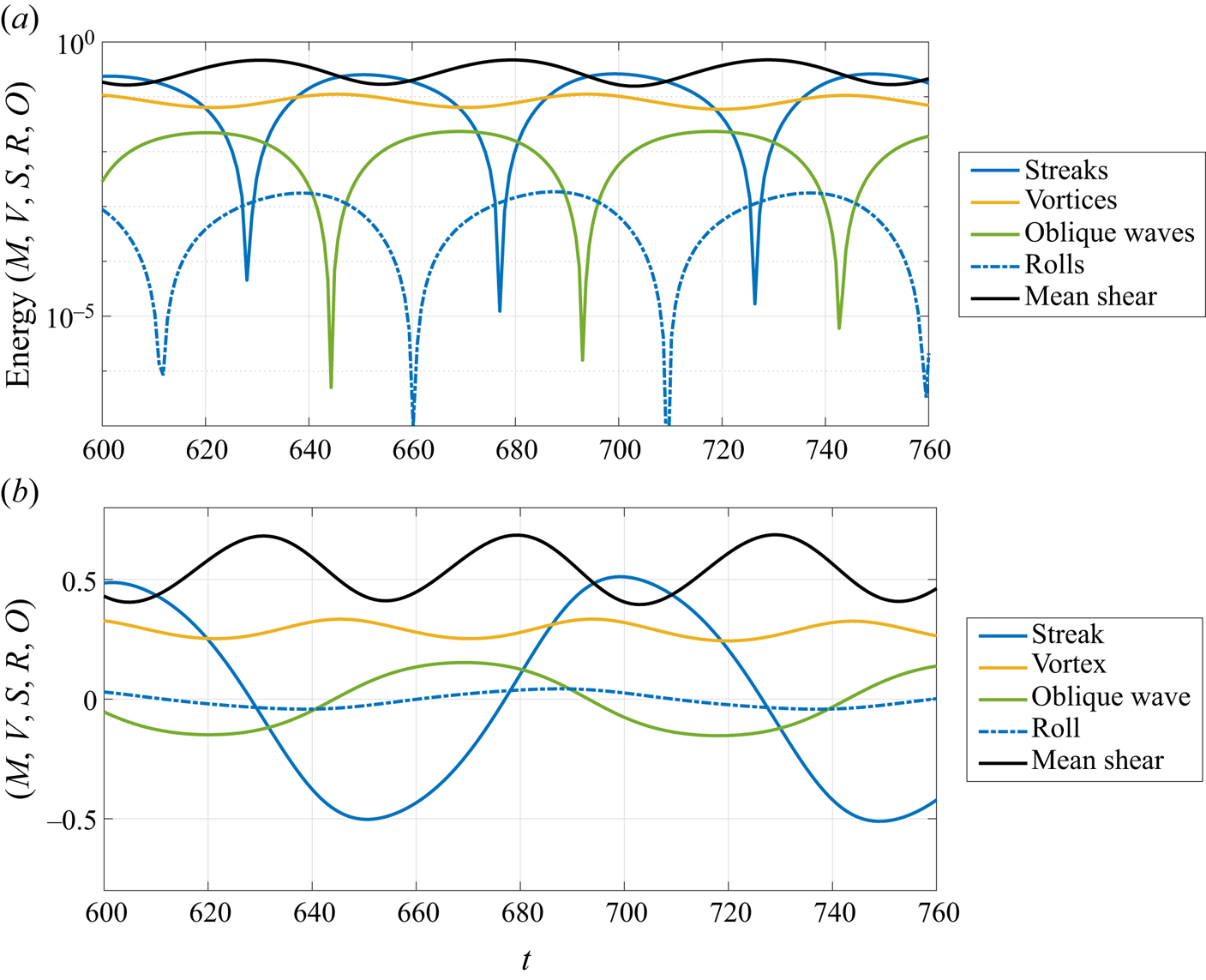
With all interactions explicitly written in the system of equations, parameters similar to Waleffe (Reference Waleffe1997) were chosen, and a limit cycle could be obtained by solving the system numerically using the ode45 function in MATLAB. After the initial transient, the simulation reaches the cycle shown in figure 1, where the parameters  $(\sigma _V,\sigma _S,\sigma _R,\sigma _O,\sigma _C)=(0.07,1.5,0.07,0.04,0.07)$,
 $(K_M,K_V,K_S,K_R,K_O)=(\sqrt {10},\sqrt {10},\sqrt {10},\sqrt {10},\sqrt {15})$ were used to simulate the dynamical system, with
 $Re = 300$. Figure 1(a) shows the energy of each mode, where the periods of growth/decay can be more clearly identified, and figure 1(b) shows the amplitude of each mode from the model, which can be seen as a metric of the relative phase of each structure. Overall, the energy of each mode follows the following dynamics: (i) vortices extract energy from the mean shear to grow in certain periods of the cycle, leading to the exponential growth of the Kelvin–Helmholtz mode; (ii) oblique waves are formed with sign defined by the sign of the streaks (such that these structures are a consequence of the interaction between
 $S$ and
 $V$); (iii) rolls are formed from the interaction between oblique waves and vortices, via the
 $\sigma _R O V$ term, which depends crucially on the sign of the oblique wave; (iv) streaks are formed from the rolls via the lift-up effect, impacting the sign of the subsequent oblique wave. We observe also that times with high amplitudes of streaks and rolls are related to stronger mean-flow distortions, reducing the value of
 $M$ which in turn modulates the vortex growth rate. Low mean-flow distortion (high
 $M$) is associated with stronger vortex growth rate, and high mean-flow distortion (low
 $M$) leads to attenuation and decay of vortices, as the instantaneous ‘mean flow’ becomes stable.

As shown in figure 1, the temporal evolution of the reduced order model leads to a limit cycle, resembling the long-established result of Hamilton et al. (Reference Hamilton, Kim and Waleffe1995), who identified a quasi-periodic behaviour involving streaks and rolls for Couette flow, computed in a small computational box. The results of figure 1 anticipate the dynamics that will be found in direct numerical simulations of a forced wall-bounded flow, which will be discussed next. Knowing that the observed limit cycle is possible in a toy model, we will focus on studying the interaction between these coherent structures in a simplified flow model (whose behaviour can be considered as representative of a mixing layer) ruled by the Navier–Stokes equations.
3. The permanently actuated, periodically unstable flow
The present work focuses on further analysing the interaction between streamwise elongated, spanwise organised structures (streaks) and Kelvin–Helmholtz-like vortices. For that, we introduce a novel flow model in which both structures are present, but with a simpler wall-bounded configuration that prevents streamwise inhomogeneity. Consider a laminar Couette flow between two walls at  $y={\pm } h$, moving with velocity
 ${\pm } U_e$. In this flow we introduce a steady forcing, independent of span and streamwise coordinates, in the shape of a hyperbolic tangent in the wall-normal direction
 $y$, such that the normalised momentum equation for the laminar solution becomes
 \begin{equation} 0=\frac{1}{Re}\frac{\partial^2 U}{\partial y^2} + P_A \tanh{\left( P_B y \right)}. \end{equation}
In the equation above, lengths and velocities are made non-dimensional using half-distance  $h$ and wall velocity
 $U_e$, respectively, which leads to a Reynolds number
 $Re=U_e h/\nu$, where
 $\nu$ is the kinematic viscosity. Choosing
 $U(\pm 1)=\pm 1$ as boundary conditions of (3.1), the laminar solution can be directly obtained as a function of the parameters
 $P_A$ and
 $P_B$, and the Reynolds number
 $Re$. The body force in (3.1) leads to positive (respectively negative) streamwise forcing for
 $y>0$ (respectively
 $y<0$), which increases velocity gradients in the central region of the flow.
For the present case, we chose  $P_A$ such that
 $\partial U / \partial y = 0$ on the walls,
 $P_B=5$ for a sharp gradient of the body force around
 $y=0$, which may nonetheless be numerically resolved with a low number of grid points, and
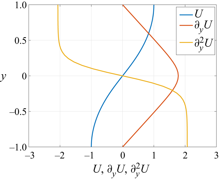
 $Re=200$. The base flow obtained from (3.1) with this choice of parameters is shown in figure 2. Similarly to laminar Couette, this is a sheared flow between two walls; still, shear is not constant as in this former flow case, but it varies throughout the domain, with a peak in the centre of the channel and zero shear at the walls. This also affects the second derivative of the base flow, which changes sign in the middle of the domain. This shows that the present flow model has an inflection point, as in mixing layers and jets, which is a necessary condition for the appearance of an inviscid instability (Rayleigh Reference Rayleigh1880), such as the Kelvin–Helmholtz mode (Michalke Reference Michalke1964). We anticipate that the present flow develops cycles of stability/instability associated to the growth/decay of a Kelvin–Helmholtz-like mode; such cycles will be related to the development of other coherent structures, such as streamwise elongated streaks, much similar to the behaviour identified for the toy model explored in § 2. Due to such characteristic behaviour, this model will be labelled as permanently actuated, periodically unstable flow, and the acronym PAPU flow will be used throughout the paper for the sake of brevity. In this framework, the PAPU number (
 $P_A$) is a metric of the deviation of the modelled base flow from the laminar Couette solution, and
 $P_B$ defines how strong the inviscid stability will be.
Base flow and its wall-normal derivatives for the present model.

In summary, PAPU flow is a sheared flow, which allows for the presence of streaks (Ellingsen & Palm Reference Ellingsen and Palm1975; Landahl Reference Landahl1980), with an inflection point that will give rise to a Kelvin–Helmholtz-like instability. Furthermore, considering that the flow is confined between two walls, a mode-by-mode analysis is straightforward in this case, as Fourier series can be taken in the streamwise and spanwise directions, which also allows for direct comparisons with the results from the toy model proposed in § 2. Also, linear models like those used in channel flows can be directly applied, reducing the usual computational cost associated to the hypothesis of streamwise varying flows. Therefore, the present model flow has the potential for isolating the interactions between the most dynamically important coherent structures, so that new insight about the turbulent dynamics in mixing layers and jets could be unveiled.
Despite the simplicity of the model, PAPU flow is a new base flow and should be appropriately characterised, especially concerning its stability and the amplification of flow disturbances. This will be accessed by means of linear stability analysis (LSA) and resolvent analysis (RA) in the next section, for the locally parallel case.
4. Linear analyses of the flow
The linearised Navier–Stokes equations expanded around  $(U(\,y),0,0)$ in the frequency–wavenumber domain can be written as
 \begin{equation} -\mathrm{i}\omega u + \mathrm{i} k_x U u + v \frac{\partial U}{\partial y}=-\mathrm{i} k_x p + \frac{1}{Re} \left( -k_x^2-k_z^2+\frac{\partial^2}{\partial y^2} \right) u + f_x, \end{equation}
 \begin{equation}-\mathrm{i}\omega v + \mathrm{i} k_x U v =- \frac{\partial p}{\partial y} + \frac{1}{Re} \left( -k_x^2-k_z^2+\frac{\partial^2}{\partial y^2} \right) v + f_y, \end{equation}
 \begin{equation}-\mathrm{i}\omega w + \mathrm{i} k_x U w =-\mathrm{i} k_z p + \frac{1}{Re} \left( -k_x^2-k_z^2+\frac{\partial^2}{\partial y^2} \right) w + f_z, \end{equation}
where  $(u,v,w)$ are the velocity components,
 $p$ is the pressure,
 $\omega$ is the frequency and
 $(k_x,k_z)$ are the streamwise and spanwise wavenumbers, respectively. The forcing terms
 $(\,f_x,f_y,f_z)$ are considered to gather the Fourier transformed nonlinear terms from the Navier–Stokes equations. Equations (4.1)–(4.3) together with the continuity equation
 \begin{equation} \mathrm{i} k_x u + \frac{\partial v}{\partial y} + \mathrm{i} k_z w = 0 \end{equation}
can be rewritten using matrix operators as
 \begin{equation} -\mathrm{i}\omega {\boldsymbol{H}} \boldsymbol{q} = {\boldsymbol{A}}\boldsymbol{q} + {\boldsymbol{B}}\boldsymbol{f}, \end{equation}
where 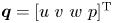 $\boldsymbol {q}=[u \ v \ w \ p]^\textrm {T}$,
 $\boldsymbol {f}=[f_x \ f_y \ f_z \ 0]^\textrm {T}$, the matrix
 ${\boldsymbol {H}}$ ensures that the time derivative is not applied to the pressure, and the matrix
 ${\boldsymbol {B}}$ ensures that the continuity equation is not violated. With the equations thus written, one can approach the problem in two ways. First, one could neglect the forcing term and look at (4.5) as an eigenproblem, looking at disturbances that will be exponentially amplified in the system; this is the focus of temporal LSA. Alternatively, one could also look at the effect of different forcing shapes in the system, and evaluate the structures that will lead to the maximum amplification between forcing and velocity. This can be done via RA. We detail these two methods in the next sections.
4.1. Temporal linear stability analysis
As mentioned earlier, temporal LSA focuses on finding flow disturbances that will be exponentially amplified in time. In summary, this method amounts to solving the eigenvalue problem defined by
 \begin{equation} -\mathrm{i}\omega {\boldsymbol{H}} \boldsymbol{q} = {\boldsymbol{A}}\boldsymbol{q}. \end{equation}
In this formulation, real-valued wavenumbers  $k_x$ and
 $k_z$ are given, and the frequency
 $\omega$ is considered to be a complex number; its imaginary part
 $\omega _i$ is the temporal growth rate of the mode, and the real part
 $\omega _r$ is related to its streamwise phase velocity
 $c$ by the expression
 $c=\omega _r/k_x$. Considering that disturbances are in the form
 \begin{equation} \tilde{\boldsymbol{q}}(t,x,y,z) = \boldsymbol{q}(\,y) \exp({-\mathrm{i}\omega t + \mathrm{i} k_x x + \mathrm{i} k_z z}), \end{equation}
eigenfunctions  $\boldsymbol {q}(\,y)$ corresponding to eigenvalues
 $\omega$ with positive imaginary part will be exponentially amplified.
Since the operator  ${\boldsymbol {A}}$ is a function of the base flow, the Reynolds number and the wavenumbers
 $(k_x,k_z)$, the stability characteristics of the flow will also be a function of these parameters. To evaluate the range of the parameters in which PAPU flow is unstable, we compute the neutral curve (the region of the space of parameters where disturbances neither grow nor decay – mathematically, the line defined by the contour
 $\omega _i=0$) for the present choice of
 $P_A$ and
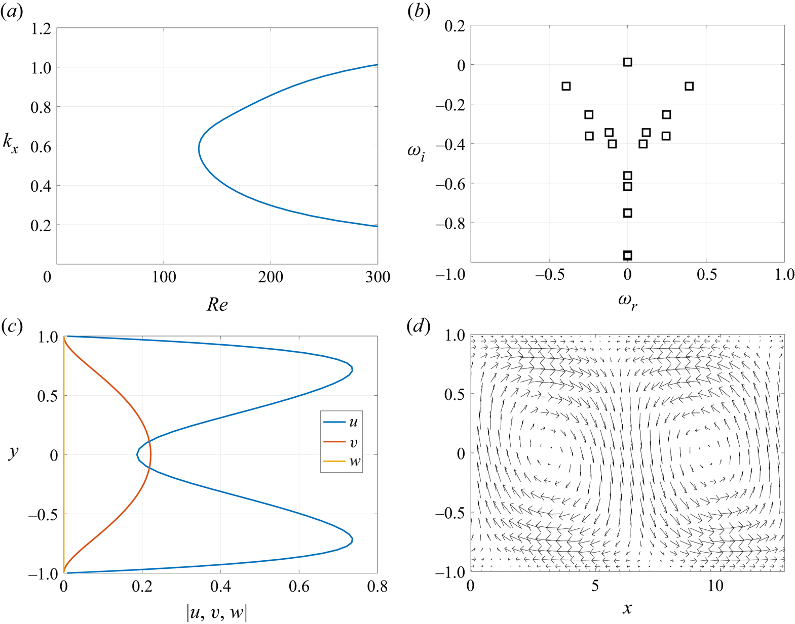
 $P_B$, shown in figure 3(a); the problem is discretised using 65 Chebyshev polynomials, following similar methods to Nogueira et al. (Reference Nogueira, Cavalieri, Jordan and Jaunet2019). The plot shows that this flow is unstable at rather low Reynolds numbers, with a critical Reynolds number of
 $Re_c=132.6$. The eigenspectrum at a sample combination of unstable wavenumbers
 $(k_x,k_z)=(0.5,0)$ at
 $Re=200$ shows that this mode has zero phase velocity (associated to
 $\omega _r = 0$), which is expected due to the zero base flow velocity at
 $y=0$, the inflection point. For this case, only one mode is unstable, with a small, positive growth rate; thus, the structure associated to this instability will be slowly (but exponentially) amplified in time.
Temporal linear stability analysis of PAPU flow. Neutral curve for the base flow parameters chosen for the analysis and  $k_z=0$ (a). Eigenspectrum for the present flow case and
 $(k_x,k_z)=(0.5,0)$ (b). Absolute value of the three velocity components of the unstable mode at
 $(k_x,k_z)=(0.5,0)$ (c) and the velocity field defined by
 $(u,v)$ for this case (d).

The shape of the unstable eigenmode for this case is shown in figure 3(c,d). As expected, due to the similarities of the present base flow to the hyperbolic tangent profile studied by Michalke (Reference Michalke1964), the resulting unstable mode displays a similar shape to this former analysis, with streamwise velocity of opposite sign at the different halves of the channel, with a phase shift in the streamwise direction. The physical shape of this mode in the  $(x,y)$ space is shown in figure 3(d). The vortical shape of the unstable mode can be clearly spotted, similar to the well-known Kelvin–Helmholtz vortices resulting from LSA applied to mixing layers. Such stationary vortices are the first coherent structure involved in the dynamics of this flow.
4.2. Resolvent analysis
Resolvent analysis has been widely used in the analysis of transition and even to evaluate the relevant parts of the turbulent dynamics in several flows. Differently from LSA, RA is developed for the forced linearised Navier–Stokes equations, such that (4.5) can be written in a input-output form as
 \begin{equation} \left[ -\mathrm{i}\omega {\boldsymbol{H}} - {\boldsymbol{A}} \right] \boldsymbol{q} = {\boldsymbol{B}}\boldsymbol{f} \Rightarrow {\boldsymbol{L}}\boldsymbol{q} = {\boldsymbol{B}}\boldsymbol{f}, \end{equation}
which, by inverting the linear operator  ${\boldsymbol {L}}$ with the appropriate boundary conditions, becomes
 \begin{equation} \boldsymbol{q} = {\boldsymbol{R}}\boldsymbol{f}, \end{equation}
and  ${\boldsymbol {R}}$ is called the resolvent operator. This is appropriate if the linearised system is stable, which occurs for the present case if the considered wavenumbers
 $k_x,k_z$ lead to a stable eigenspectrum in linear stability analysis.
By performing a singular value decomposition of this operator  ${\boldsymbol {R}}={\boldsymbol {U}} {\boldsymbol {\varSigma }} {\boldsymbol {V}}^H$ (where the superscript
 $H$ indicates the trans-conjugate), optimal bases for forcing and response are obtained in the columns of
 ${\boldsymbol {V}}$ and
 ${\boldsymbol {U}}$, respectively, and each of these modes are related to each other by gains in the diagonal matrix
 ${\boldsymbol {\varSigma }}$. Therefore, optimal forcing and the associated response are directly obtained by isolating the mode with maximum gain
 $\sigma _1$. Also, by evaluating
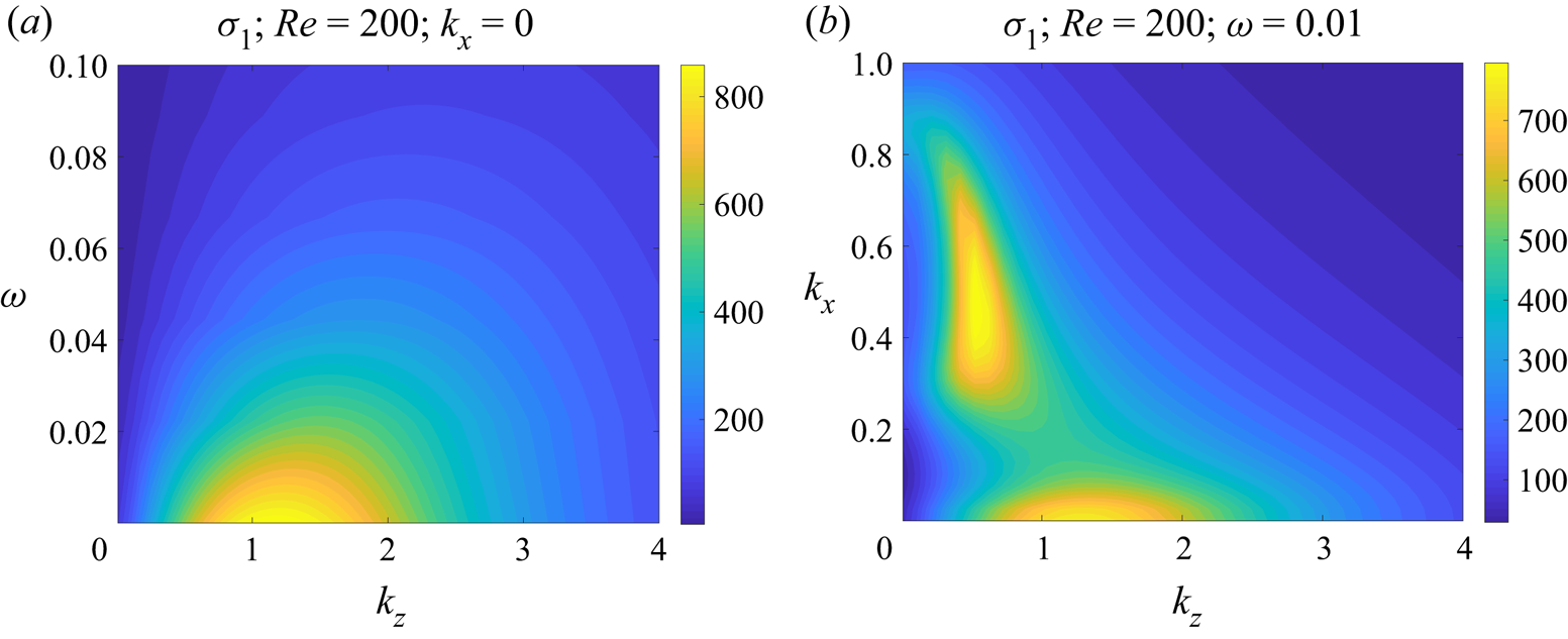
 $\sigma _1(\omega ,k_x,k_z)$, the most responsive combination of frequencies and wavenumbers can be identified for a given flow, which can be potentially important for the identification of the underlying physical mechanisms. Considering that PAPU flow is a modification of the standard Couette profile, it is expected that optimal forcing and responses would be found for very low frequency and streamwise wavenumber, which is associated to the lift-up effect and to the appearance of streaks in this flow (Schmid & Henningson Reference Schmid and Henningson2001; Brandt Reference Brandt2014). This is confirmed in figure 4(a), which shows that large gains are found for
 $\omega = k_x = 0$ (with a peak around
 $k_z=1.15$). Looking at the gains as a function of
 $(k_x,k_z)$ for
 $\omega \to 0$ in figure 4(b), the same amplified region is found for
 $k_x=0$ and
 $k_z \approx 1.2$, pointing to a mechanism in which forcing and response are spanwise organised and elongated in the streamwise direction, with a slow time dynamics. Another energetic region can be found in the range
 $0.3 \leqslant k_x \leqslant 0.7$ and
 $k_z \approx 0.5$ for
 $\omega \to 0$. These potentially energetic modes are related to oblique waves, suggesting that these structures might also play a role in the dynamics of this flow. Interestingly, the most responsive regions of the spectra predicted by RA are close to the most energetic regions of the spectra of a turbulent jet (Nogueira et al. Reference Nogueira, Cavalieri, Jordan and Jaunet2019), highlighting similarities between this flow model and a real turbulent flow.
First resolvent gain as a function of  $\omega$ and
 $k_z$ for
 $k_x=0$ (a) and the same quantity as a function of
 $k_x$ and
 $k_z$ for
 $\omega =0.01$ and
 $Re=200$ (b).

From figure 4, it is clear that  $\omega =k_x=0$ and
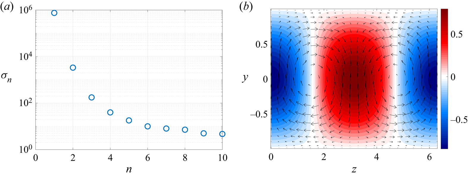
 $k_z=1$ is associated to one of the most dominant modes of the flow response, and is thus a combination of wavenumbers relevant for the flow dynamics. Figure 5(a) shows the 10 first gains from RA for this case; there is a substantial separation between optimal and suboptimal gains, suggesting that the mechanism associated to the first resolvent gain is dominant in this case. Figure 5(b) shows that the response mode for this case assumes the shape of streaks in the streamwise velocity, and rolls (streamwise vortices) in the
 $(v,w)$ field. Considering that this is a sheared flow, the presence of such structures is expected due to the lift-up effect, where streaks are created by advection of the sheared base flow by the rolls (Ellingsen & Palm Reference Ellingsen and Palm1975; Landahl Reference Landahl1980). Streaks and rolls are the second and third coherent structures in PAPU flow, and these will interact with the vortices (predicted by LSA) and with energetic oblique waves to determine some of the relevant flow processes.
Gains from resolvent analysis (a) and the equivalent optimal response mode (b) for  $k_z=1$,
 $k_x=0$ and
 $\omega =0$.

In summary, PAPU flow encompasses four of the most important coherent structures of turbulent free-shear flows: Kelvin–Helmholtz-like vortices, streaks, rolls and oblique waves; considering that the same structures are present in mixing layers and jets, this model can potentially reproduce part of the turbulent dynamics of such flows. Moreover, the analysis is simplified by the fact that the present flow is confined between two walls, so that the interactions between all of these can be directly examined in a reduced order model or a direct numerical simulation with low computational expense as in Hamilton et al. (Reference Hamilton, Kim and Waleffe1995); Waleffe (Reference Waleffe1995, Reference Waleffe1997). This will be performed in the next sections.
5. Direct numerical simulation
5.1. Choice of computational domain
In order to perform a direct numerical simulation of PAPU flow for the case described in § 3 we start from the laminar solution of Couette flow at  $Re=200$, which is known to be linearly stable for any initial disturbance. Starting from this laminar solution, a spatially distributed body forcing in the shape of a hyperbolic tangent, as in (3.1), is introduced permanently in the flow, so that the steady-state, laminar solution assumes the shape seen in figure 2. The present simulation was performed in SIMSON (Chevalier, Lundbladh & Henningson Reference Chevalier, Lundbladh and Henningson2007) with
 $(N_x,N_y,N_z)=(32,65,32)$ collocation points before dealiasing. The code numerically solves the incompressible Navier–Stokes equations, discretised using Fourier modes, in both spanwise and streamwise directions, and Chebyshev polynomials in the wall-normal direction. A four-stage Runge–Kutta method, with an adaptive time step in order to satisfy a maximum Courant–Friedrichs–Lewy number of
 $0.5$, was chosen as a time advancement scheme, and the physical fields were stored at rate
 ${\rm \Delta} t=1$. The box size was chosen based on the results of § 4: since we are interested in evaluating the interaction between vortices, streaks and other structures, the box should allow for the growth of the unstable mode at this Reynolds number. Therefore, a box size of
 $(L_x,L_y,L_z)=(4{\rm \pi} , 2 , 2{\rm \pi} )$ was chosen, enabling the growth of modes associated to
 $k_x=0.5$, which is unstable for this case. The box size also enables structures related to
 $(k_x,k_z)=(0,1)$, which are related to the energetic streaks found in figures 4 and 5. The simulation is started with spatial white noise, which triggers the instability. Due to the reduced Reynolds number and the box size, the simulation does not lead to turbulence; instead, the flow enters a limit cycle, with the coherent structures interacting in such a way to keep the flow in a stable cycle.
5.2. Basic properties of the numerical solution
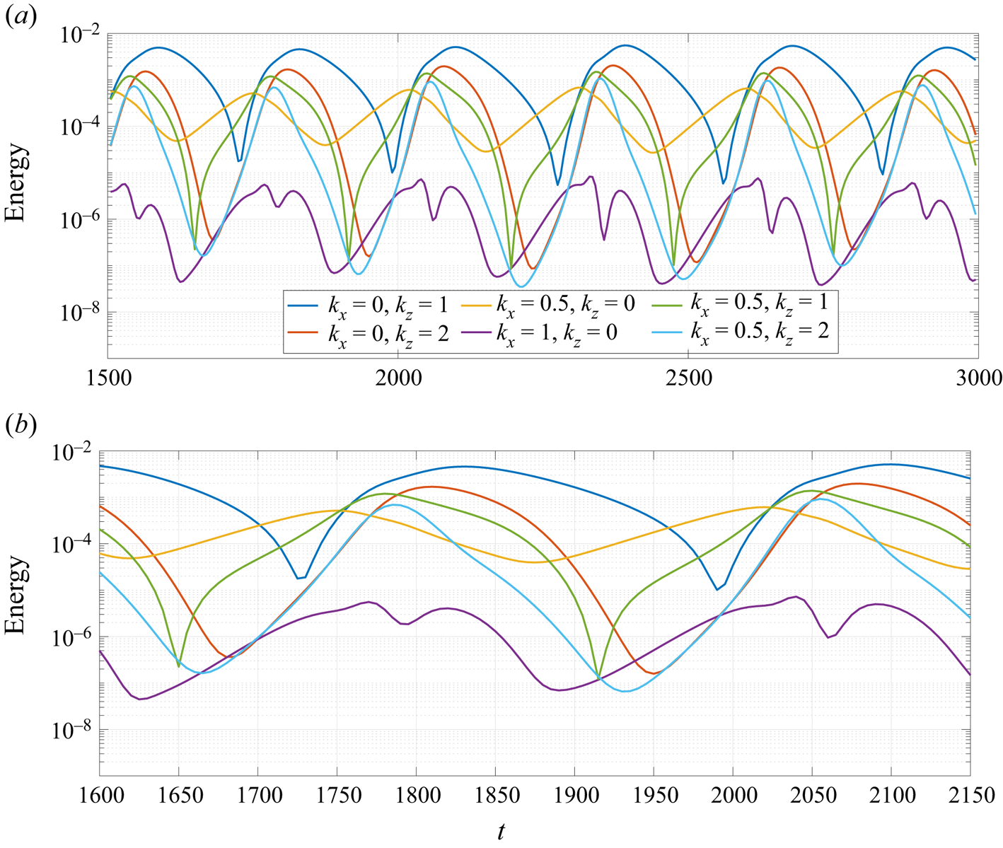
The energy related to the most relevant combination of wavenumbers in the observed limit cycle as a function of time can be seen in figure 6. Clearly, the streaky mode  $(k_x,k_z)=(0,1)$ has most of the energy of this flow for almost all times, with some regions of sharp decay, suggesting an intermittent cancellation of this mode. The vortex, i.e.
 $(k_x,k_z)=(0.5,0)$, on the other hand, has intervals of exponential growth and decay, and is never totally damped in the flow. Other modes are also important in the flow dynamics: the oblique wave mode
 $(0.5,1)$, for instance, has a higher energy growth at some times compared to the vortex mode, even though it is also subject to a cancellation at other parts of the cycle; similar phenomena occur for modes
 $(0.5,2)$ and
 $(0,2)$. The energy of the second two-dimensional mode (
 $k_x=1$ and
 $k_z=0$) is several orders of magnitude lower than the other modes at most of the times, and does not seem to play a significant role in the observed dynamics.
Energy of the modes related to the most relevant combination of wavenumbers in the limit cycle for several periods (a) and a single (minimal) period (b). The main structures associated to the combination of wavenumbers  $(k_x,k_z)$ are streaks and rolls
 $(0,1)$, vortices
 $(0.5,0)$ and oblique waves
 $(0.5,1)$.

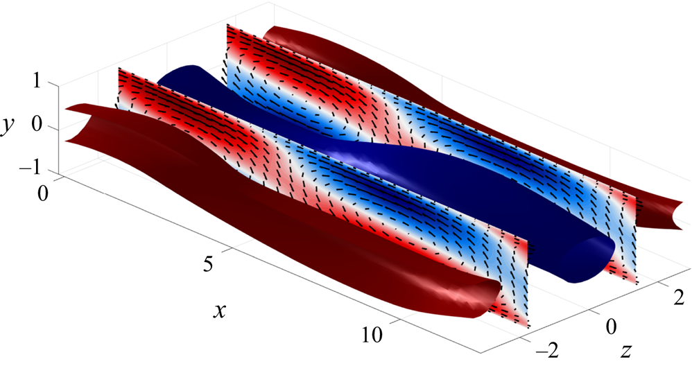
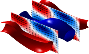
The importance of streaks and vortices in the flow is reinforced by simply looking at the streamwise/wall-normal velocity field at a given simulation time. Isocontours of 60 % of maximum streamwise velocity at  $t=1930$ are shown in figure 7, and streaky structures similar to the ones found in the analysis of Hamilton et al. (Reference Hamilton, Kim and Waleffe1995) can be clearly spotted; the high energy of such structures facilitate their identification in the raw velocity field. At this time, vortices are less energetic, and can only be seen by taking the spanwise mean of the velocity field. Contours of this structure are depicted in the slices shown in figure 7.
Isocontours of 60 % of positive (red) and negative (blue) maximum streamwise velocity at  $t=1930$. Slices show the field resulting from the spanwise average of the velocity at
 $t=1930$, where vortices can be clearly spotted. Colours indicate streamwise velocity fluctuations and arrows depict streamwise and wall-normal velocity fluctuations.

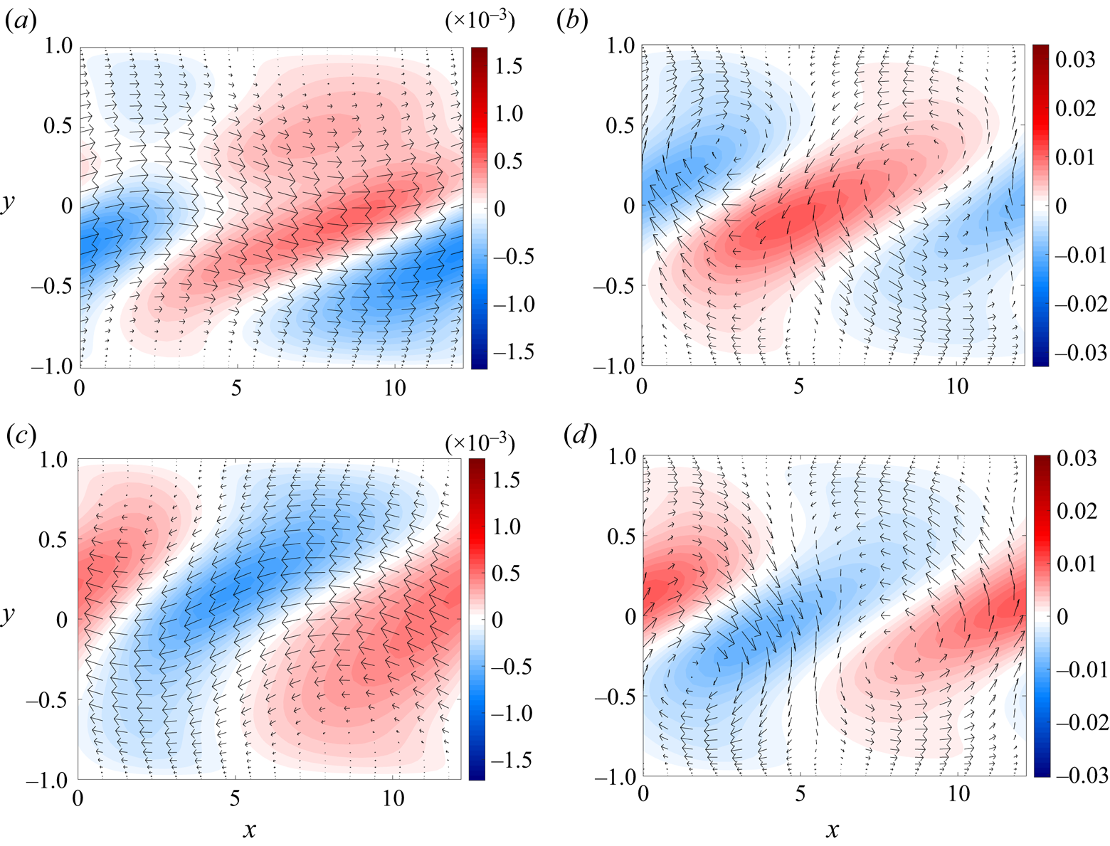
This coupled movement of streaks and vortices can be perceived in the velocity fluctuation fields at different times, as shown in figure 8. Initially ( $t=1650$) an energetic positive streak arises in the mid-span (
 $z=0$), as illustrated in figure 8(a). At this time, the vortex is unstable, but still has low energy (see figure 6b), and cannot be directly identified in the instantaneous velocity field, without a spanwise average. Vortex growth is associated to a decay on the streak amplitude so that, around
 $t=1730$ (figure 8b), this Kelvin–Helmholtz-like structure becomes visible in the field for some time. Saturation and decay of the vortex occurs after the emergence of a negative streak at
 $z=0$ (seen at
 $t=1920$, for example) cancelling the previous streaky structure, thus explaining the sharp valley in the energy of mode
 $(k_x,k_z)=(0,1)$ in figure 6. There is thus a time-periodic shift of the spanwise phase of streaks, which jump between
 $0$ and
 ${\rm \pi}$; this is a relevant feature of the cycle that will be further explored later. The cycle is, then, restarted at a different phase, defined by the new phase of the streak, giving rise to new vortices with the same phase as the previous ones, but at a different wall-normal position, as shown in figure 8(d). This vortex movement due to the streak was also identified by Pierrehumbert & Widnall (Reference Pierrehumbert and Widnall1982) for a periodic mixing layer and was, at the time, associated to the presence of a translative instability. This mechanism would tend to move the vortices in the
 $y$–
 $z$ directions and generate large-scale streaks that would grow in space for long distances.
Snapshots of velocity fluctuation fields at a plane  $x$–
 $y$ located at the mid-span (
 $z=0$) for different simulation times: (a)
 $t = 1650$, (b)
 $t = 1730$, (c)
 $t = 1920$ and (d)
 $t = 2000$. Colours represent spanwise velocity and arrows depict the streamwise/wall-normal velocity.

Thus, the DNS of PAPU flow for the present small computational box leads to vortex dynamics with position changing in  $y$ and with varying amplitude in time. Despite the high level of organisation of these results, a connection can be made clearly with the phenomenon of jitter in turbulent jets: for such flows, the Kelvin–Helmholtz wavepacket is subject to phase jumps, amplitude variation and energy bursts that cannot be reproduced in frequency domain models without using two-point flow statistics (or models that capture some of the features of these quantities) (Cavalieri et al. Reference Cavalieri, Jordan, Agarwal and Gervais2011, Reference Cavalieri, Rodríguez, Jordan, Colonius and Gervais2013). The relationship between jitter and coherence decay was developed by Cavalieri & Agarwal (Reference Cavalieri and Agarwal2014), who has shown that jittering wavepackets in time will lead to wavepackets with a coherence envelope in the frequency domain, which greatly affects the sound generation by these structures. Comparison of the space–time signal of the vortices at
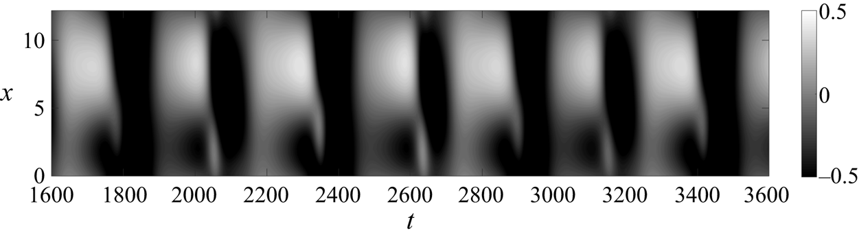
 $(\,y,z)=(-0.5,{\rm \pi} /2)$, a position where vortices can be seen more clearly, shown in figure 9, leads to features that are also observed in turbulent jets (Cavalieri et al. Reference Cavalieri, Jordan, Agarwal and Gervais2011; Breakey et al. Reference Breakey, Jordan, Cavalieri, Nogueira, Léon, Colonius and Rodríguez2017), with amplitudes varying with time for a given streamwise position for this stationary vortex. Considering that only one pair of energetic streaks is observed in the simulation, this quantity still has a high level of organisation in time, but the inclusion of other streaks (by increasing the box size in
 $z$) is expected to lead to a more random behaviour; initial simulation results confirm this hypothesis.
Streamwise velocity at  $(\,y,z)=(-0.5,{\rm \pi} /2)$ as a function of time and
 $x$. Time-varying dark and white regions point to the presence of positive and negative streaks (clear or dark bands for a given
 $t$, such as for
 $t=2400$) modulating the vortices amplitudes, which can be seen as bands with positive and negative streamwise velocity (e.g. at
 $t=2000$).

At this point, we have used locally parallel analyses to evaluate the relevant frequencies and wavenumbers related to the appearance of coherent structures in this model flow. These results were used to design the computational box for the analysis of the interaction between these structures, and results from DNS show the existence of a limit cycle involving a small number of modes. This cycle was shown to reproduce some of the characteristics of mixing layers and turbulent jets, suggesting that some of the dynamical interactions of such flows are also present in PAPU flow. Also, the energy of the most relevant modes in the cycle of figure 6 follows qualitatively the behaviour of the equivalent modes of the toy model explored in § 2 (shown in figure 1). This points out that the interactions explicitly postulated in (2.1)–(2.5) might be at play in the present simulation, and that the proposed model can be useful in the study of these coherent structures. We proceed now to a more detailed analysis of the growth/decay mechanism of the dominant structures in this cycle.
5.3. The limit cycle
5.3.1. Step 1: vortex growth
We start by analysing the growth/decay mechanism of the Kelvin–Helmholtz-like vortices. Linear stability analysis results, presented in § 4.1, shows that laminar PAPU flow is unstable for  $Re=200$ and
 $k_x=0.5$, leading to the growth of vortices. Still, the mean flow from the DNS does not necessarily enable the growth of such mode at all times. This can be accessed by performing the linear stability analysis using the mean flow from the simulation (with the mean taken in span and streamwise directions) at each time step. This provides an estimation of the regions of growth, saturation and decay of the mode, considering that this mechanism is strictly linear, with energy being transferred only from the mean flow to the unstable mode.
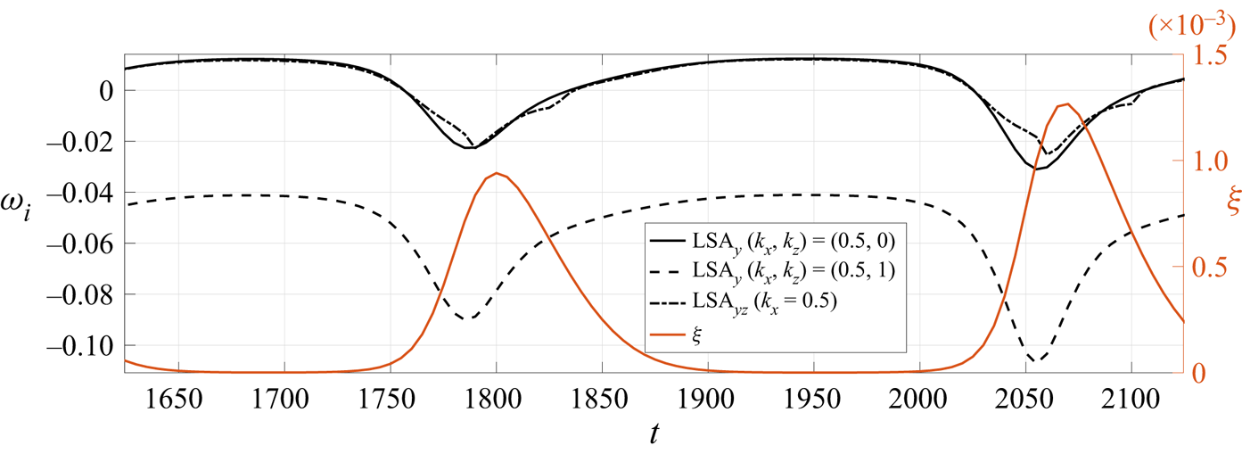
The black lines in figure 10 shows the growth rate of the most unstable mode for several cases: solid and dashed lines are results from locally parallel analysis for  $(k_x,k_z)=(0.5,0)$ and
 $(0.5,1)$, considering a mean flow averaged in both streamwise and spanwise directions; the dash–dot line represents the growth rate from LSA using the Navier–Stokes equations linearised around the streamwise averaged flow
 $(U(\,y,z), V(\,y,z), W(\,y,z))$ for
 $k_x=0.5$; the latter analysis is carried out using the same Fourier–Chebyshev discretisation of the DNS. The orange line (and the equivalent
 $y$-axis on the right) shows the integrated square of the deviations between mean flow
 $\bar {U}(\,y)$ and the laminar solution
 $U(\,y)$, given by
 \begin{equation} \xi(t) = \int_{-1}^1 \left( \bar{U}(\,y) - U \right)^2 \mathrm{d} y. \end{equation}
It is thus a metric of mean-flow distortion, related to Reynolds stresses induced by the various flow structures. Comparing figures 10 and 6, it is clear that the locally parallel stability analysis performed using the mean flow from the simulation predicts well the regions of growth ( $\omega _i > 0$) and decay (
 $\omega _i < 0$) of the vortical structure. A slight delay between the time in which the mode becomes unstable and the actual growth of the mode in the DNS, also identified in figure 10, might be caused by the interaction between the existing decaying mode and the newly amplified mode in the flow. Figure 10 also shows a clear association between the saturation of the instability and the deviations of the mean flow from the laminar solution: when mean-flow distortion is small, the flow follows the predicted instability mechanism. After some time, distortion
 $\xi$ increases greatly, with the mean flow receiving energy from the nonlinear interactions of several modes via Reynolds stresses, thus leading to a stabilisation of the vortices. Afterwards, when all modes are decaying, the deviations from the laminar solution also decay, triggering the instability once again and restarting the semi-cycle. Similar features were seen in the toy model of § 2, where mean-flow distortion (changes in
 $M$) modify the growth rate of the vortices
 $V$, as clear in (2.6).
Imaginary part of the frequency of the most unstable mode from linear stability analysis using the mean flow from the simulation. Solid and dashed black lines are results from the locally parallel analysis for  $(k_x,k_z)=(0.5,0)$ and
 $(k_x,k_z)=(0.5,1)$. The dash–dot line is the result of the bi-dimensional case, where the mean flow is a function of
 $(\,y,z)$ for
 $k_x=0.5$. The right
 $y$-axis (in orange) shows a metric for the deviations of the mean flow
 $U(\,y)$ from the laminar case.

5.3.2. Step 2: growth of oblique waves
Differently from the vortices, the oblique waves do not follow an instability mechanism for a base flow depending only on  $y$; as shown in figure 10, mode
 $(k_x,k_z)=(0.5,1)$ has
 $\omega _i<0$ for all times of the cycle, meaning that this mode should be decaying in this framework. In order to evaluate if the growth of this mode is associated to the tri-dimensionality of the mean flow, we analyse the results from LSA of the streamwise averaged flow for
 $k_x=0.5$, shown by the dash–dot line of figure 10; modes resulting from this analysis can include any combination of wavenumbers
 $(k_x, k_z) = (0.5; 2 {\rm \pi}n_z/L_z)$, where
 $n_z$ is an integer. Results from this analysis predict the same intervals for growth and decay of fluctuations, suggesting that wavenumber
 $(k_x,k_z)=(0.5,0)$ is dominant in the unstable eigenfunction. The present results can be related to the findings of Marant & Cossu (Reference Marant and Cossu2018), whose stability analysis of a streaky shear layer shows that a stabilising effect of streaks occurs through a distortion of the spanwise average of the flow.
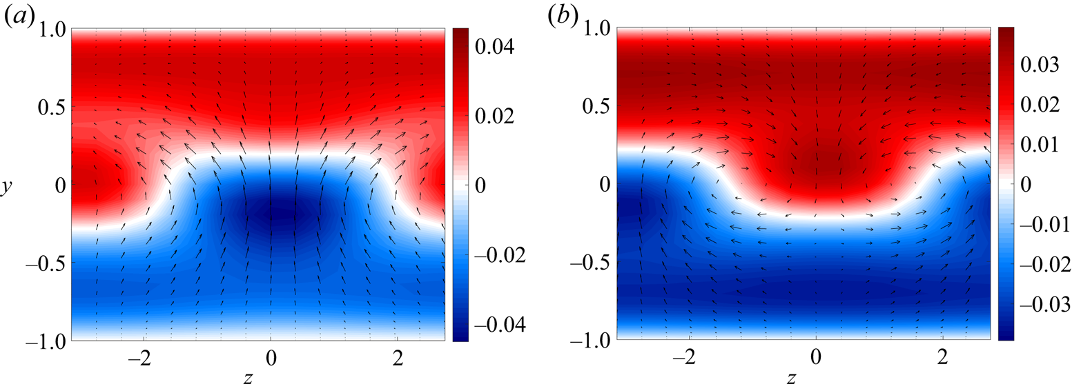
The unstable mode from this analysis at different times of the cycle is shown in figure 11. The structure is clearly dominated by the  $k_z=0$ mode, especially closer to the walls. Still, closer to the centre of the channel, the eigenmode assumes a tri-dimensional shape, with a spanwise variation corresponding to
 $k_z=1$. The streaky mean flow thus couples the growth of vortices –
 $(0.5,0)$ wavenumber – and oblique waves –
 $(0.5,1)$ wavenumber, which are both contained in the unstable eigenfunction. Moreover, the streak configuration in the mean flow anchors the phase of oblique waves in the unstable eigenfunction. This can be seen in the phase shift between figures 11(a) and 11(b): for
 $t=1650$, a positive streak is located at
 $z=0$ (as shown in figure 8a), and the resulting eigenmode has a positive wall-normal velocity at this position. At
 $t=1920$ (figure 8c), the negative streak assumes that position, and the phase of the unstable oblique wave is shifted in
 $z$.
Real part of the most unstable mode from LSA of a streamwise averaged flow for  $k_x=0.5$ at two time steps: (a)
 $t=1650$ and (b)
 $t=1920$. Contours depict streamwise velocity fluctuations and arrows show the wall-normal/spanwise velocity fields.

Therefore, the coupled growth of vortices and oblique waves can be explained by means of linear stability analysis of the streamwise averaged flow. For the case of oblique waves, a streaky base flow is needed to trigger the instability, so that the resulting eigenmode has a spanwise phase defined by the position of the positive/negative streak in the flow. This feature is also present in the toy model of § 2, as clear in the linear stability analysis of a ‘streaky’ base flow in (2.7)–(2.8). Notice that in the toy model the relationship between vortices  $V$ and oblique waves
 $O$ depends on the phase of the streaks (represented in the model by the sign of
 $S$). Still, the back effect of the growth of these modes in the streaks cannot be directly obtained by this linear analysis for PAPU flow, especially if one hopes to explain the change of phase of these structures in the cycle. This phenomenon will be explained in the next section using the data from the numerical simulation.
5.3.3. Step 3: cancellation and phase shift of streaks
As shown in figures 8(a) and 8(c), positive and negative streaks associated to mode  $(k_x,k_z)=(0,1)$ are alternating their position in the domain, defining the phase of the oblique wave at each part of the cycle. Such streaks are often associated to the lift-up effect which can be summarised as follows: in the presence of rolls (streamwise vortices), positive wall-normal velocity transfers momentum from low- to high-speed regions of the fluid; the coupling of this velocity component to the shear in the streamwise momentum equation induces a velocity defect so that a negative streak is generated, with the opposite happening for a positive streak. Lift-up can also be seen in the forced problem as a process in which rolls in the forcing field generate rolls in the velocity field, and these will lead to the resulting streaky flow. With that in mind, we can analyse the results from the simulation in this framework.
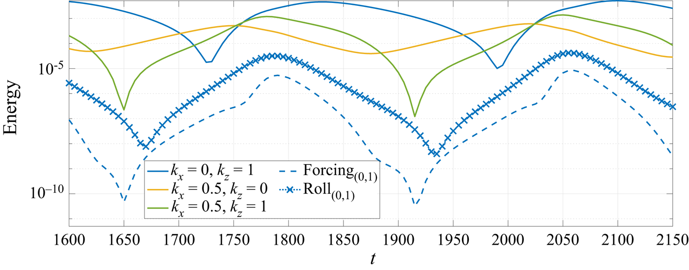
Figure 12 reproduces the energy of each of the most energetic modes in the minimal cycle of PAPU flow. In the same plot, we show the energy related to the rolls (defined as the energy of the related to the  $(v,w)$ field of mode
 $(k_x,k_z)=(0,1)$) and the energy of nonlinear forcing term for the same combination of wavenumbers. These are computed in the physical domain from the DNS as
 \begin{equation} \boldsymbol{f}=-(\boldsymbol{u}\boldsymbol{\cdot} \boldsymbol{\nabla})\boldsymbol{u} , \end{equation}
where  $\boldsymbol {u}=(u,v,w)$ is the velocity fluctuation vector. This resulting field is then Fourier transformed in
 $x$ and
 $z$, in order to obtain the forcing for each mode. Such field
 $\boldsymbol {f}$ thus corresponds to the forcing term in the analysis of turbulent flows using the resolvent operator (McKeon & Sharma Reference McKeon and Sharma2010), and the main results from resolvent analysis (Hwang & Cossu Reference Hwang and Cossu2010; Nogueira et al. Reference Nogueira, Morra, Martini, Cavalieri and Henningson2020) may be used to interpret the effect of
 $f$ on flow responses. Looking at the beginning of the cycle, the forcing energy of mode
 $(0,1)$ starts to grow after a sudden drop. Some time steps later, the same phenomenon occurs for the energy of the rolls and afterwards for the streaks (which dominate the energy of mode
 $(0,1)$). Forcing and roll follow the same overall behaviour in time.
Energy of the different modes involved in the dynamics of PAPU as a function of time. The dashed line represents the energy related to the forcing of mode  $(0,1)$ and the symbols depict the energy related to the
 $(v,w)$ velocity field of mode
 $(0,1)$, i.e. the energy of rolls. With solid lines, wavenumbers
 $(k_x,k_z)$ represent the energy of streaks
 $(0,1)$, vortices
 $(0.5,0)$ and oblique waves
 $(0.5,1)$.

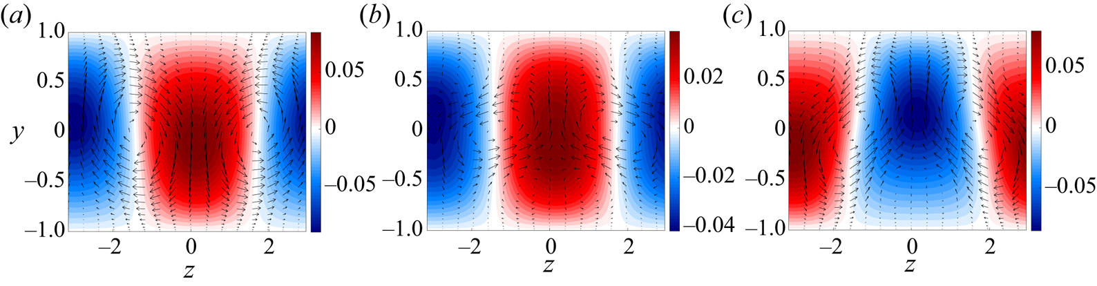
The sharp changes in the energy of the modes of figure 12 can be better understood by looking at the streamwise averaged velocity field, which will be dominated by mode  $(0,1)$ for almost all times. These fields at some relevant times can be seen in figure 13. At
 $t=1650$, rolls and streaks are present in the flow in a lift-up configuration, with negative wall-normal velocity associated to a positive streak and vice versa. After the sudden decay of rolls (for a time when such structures are growing), the orientation of these rolls is changed, such that streaks and rolls stand in an ‘anti-lift-up’ configuration; we will refer to this as formed by streaks and anti-rolls, as the latter are phase shifted in a way that is expected to cancel the former. Due to the lift-up effect, these anti-rolls thus progressively generate streaks with the opposite sign of the previous ones (anti-streaks), which cancel the previous ones. Finally, after the sharp valley of streak amplitude (associated to this cancellation), the flow is dominated by anti-rolls and anti-streaks (as in
 $t=1900$) with the ‘correct’ spanwise phase relationship, restoring the standard lift-up configuration.
Streamwise averaged ( $k_x=0$) velocity field at several times: (a)
 $t=1650$, (b)
 $t=1690$ and (c)
 $t=1900$. Laminar solution was removed from the field to show the streaks more clearly. Colours: streamwise velocity. Arrows: wall-normal/spanwise velocity field.

Lift-up is a robust mechanism in shear flows (Brandt Reference Brandt2014), and is a key feature of the dynamics of PAPU flow. It is clear from several works (Hamilton et al. Reference Hamilton, Kim and Waleffe1995; Del Alamo & Jimenez Reference Del Alamo and Jimenez2006; Hwang & Cossu Reference Hwang and Cossu2010; Farrell & Ioannou Reference Farrell and Ioannou2012) that the time evolution of the most energetic structures in the flow (streaks) are a consequence of the dynamics of rolls, even though the latter have much lower energy; this is due to a non-normal amplification of streamwise-independent disturbances (Landahl Reference Landahl1980; Butler & Farrell Reference Butler and Farrell1992). The alternation between streaks and anti-streaks can be easily explained by the evolution of the rolls, as the inversion of roll circulation for a given  $z$ tends to cancel the current streak and produce a new one of opposite sign. The process of rolls turning into anti-rolls is more intricate, but the temporal evolution of the forcing related to that mode provide some indications of the underlying mechanism. The toy problem of § 2 is again a useful illustration of the observed behaviour. Equation (2.4) has roll dynamics that are forced by an interaction between oblique waves
 $O$ and vortices
 $V$. As
 $V>0$ for all times, the sign of the forcing term depends on the sign of the oblique waves, which may reinforce (if
 $O$ and
 $R$ have the same sign) or cancel rolls (if
 $O$ and
 $R$ have opposite signs). The change in sign of
 $O$ in figure 1 is related to the beginning of a cancellation of rolls, which decay to zero amplitude and then reappear with opposite sign.
We will now show that a similar mechanism is at play in the direct numerical simulation of PAPU flow. In figure 12 the cancellation of the oblique wave  $(0.5,1)$ happens at the same time of the sharp decay of the forcing of mode
 $(0,1)$; also, this forcing follows the growth of modes
 $(0.5,0)$ and
 $(0.5,1)$, suggesting that the nonlinear interaction between these two modes may be the most relevant component of this forcing term. To analyse that, we compute the triadic interaction between these two modes that lead to the forcing at wavenumbers
 $(k_x,k_z)=(0,1)$ (namely, the interactions between the velocity fields of modes
 $(\pm 0.5,0)$ and
 $(\mp 0.5,1)$), which is given by the expression
 \begin{align} \boldsymbol{f}_{triadic}^{0,1}&=-(\boldsymbol{u}^{-0.5,0}\boldsymbol{\cdot}\boldsymbol{\nabla}) \boldsymbol{u}^{0.5,1} -(\boldsymbol{u}^{0.5,1}\boldsymbol{\cdot} \boldsymbol{\nabla})\boldsymbol{u}^{-0.5,0} \nonumber\\ &\quad -(\boldsymbol{u}^{0.5,0}\boldsymbol{\cdot} \boldsymbol{\nabla})\boldsymbol{u}^{-0.5,1} -( \boldsymbol{u}^{-0.5,1}\boldsymbol{\cdot} \boldsymbol{\nabla})\boldsymbol{u}^{0.5,0}, \end{align}
where the superscripts indicate the combination of wavenumbers of each mode. In order to extract the most dynamically relevant part of the forcing fields, we also perform a Helmholtz decomposition, such that the forcing is written as a sum of an irrotational (curl-free) field  $\boldsymbol {\nabla } \times \boldsymbol {F}_{irr}$ and its solenoidal (divergence-free) counterpart
 $\boldsymbol {\nabla } \phi _{sol}$ as
 \begin{equation} \boldsymbol{f} = \underbrace{\boldsymbol{\nabla} \times \boldsymbol{F}_{irr}}_{\boldsymbol{f}_{irr}} + \underbrace{\boldsymbol{\nabla} \phi_{sol}}_{\boldsymbol{f}_{sol}}. \end{equation}
Analysis of the Navier–Stokes operators shows that only the solenoidal part of the forcing leads to a response in the velocity field of incompressible flows (Jovanovic & Bamieh Reference Jovanovic and Bamieh2005; Rosenberg & McKeon Reference Rosenberg and McKeon2019); thus, it is sufficient to analyse the divergence-free part of the forcing. This also eliminates irrelevant parts of the forcing (the ones that generate no response in the velocity), clearing the field such that coherent structures could be more clearly spotted.
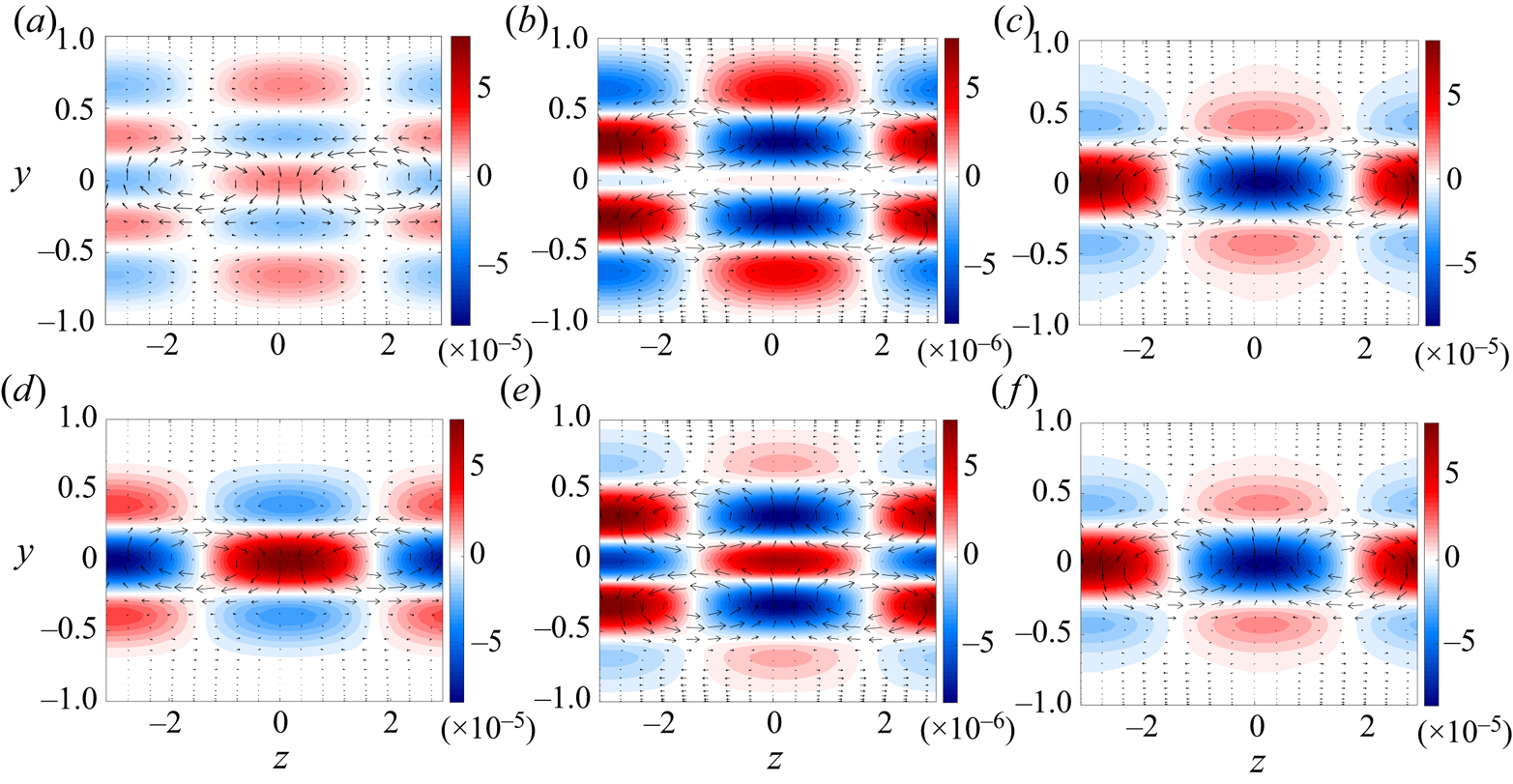
The solenoidal forcing field of mode  $(0,1)$, computed from the DNS for the times around the sharp decay of the forcing, is shown in figure 14(a–c). At initial times (
 $t=1630$), before the minimum of the forcing, rolls can be identified in the data (figure 14a), acting in the same direction as the rolls in the velocity field (figure 13a), reinforcing the lift-up effect. Precisely at the time of minimal amplitude (
 $t=1650$), new forcing rolls are induced in the field, doubling the previous structure in the wall-normal direction (figure 14b). A forcing anti-roll is seen for subsequent times; at
 $t=1670$, for instance, this new structure can already be seen in the field (figure 14c). Since such a structure acts on mode
 $(0,1)$, this forcing will lead to the rise of the anti-roll in the velocity field (figure 13b), explaining how this alternation is started. The forcing fields can also be compared with the ones coming from the triadic interactions between modes
 $(0.5,0)$ and
 $(0.5,1)$, shown in figure 14(d–f). These plots show that forcing rolls from this single triadic interaction follow exactly the same trend as the full forcing of mode
 $(0,1)$, which indicates that the nonlinear interaction between the vortices and the oblique waves is responsible for the change of sign of the forcing rolls, leading to the alternation between rolls and anti-rolls in the velocity field. This also explains the coupled behaviour between the energy growth of mode
 $(0.5,1)$ and the forcing
 $(0,1)$ in figure 12: since this component of the forcing is directly influenced by the oblique wave and the vortices, its energy will also be related to the energy of such modes.
Solenoidal part of the  $(0,1)$ component of the forcing from all nonlinear terms (a–c) and from the triadic interations between modes
 $(0.5,1)$ and
 $(0.5,0)$ (d–f): (a,d)
 $t=1630$; (b,e)
 $t=1650$; (c,f)
 $t=1670$. Colours: streamwise forcing. Arrows: wall-normal/spanwise forcing field.

5.4. Overview of the dynamics
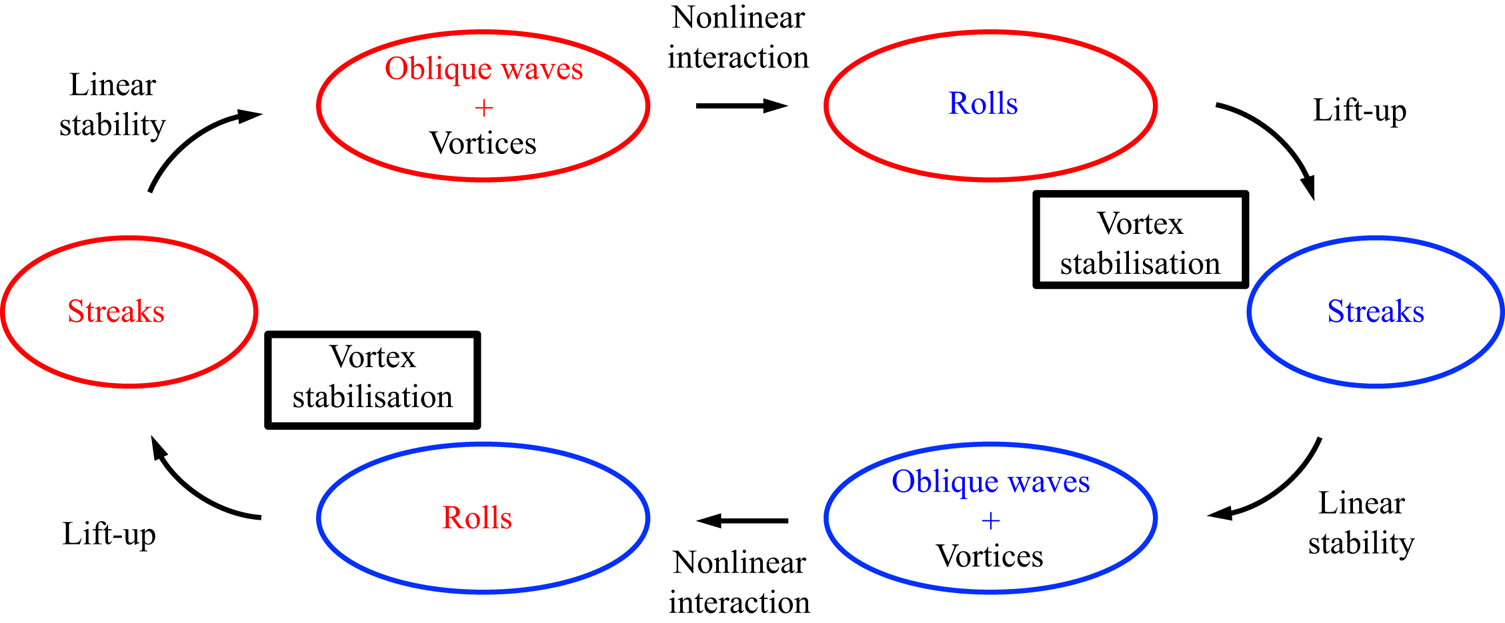
The analysis of §§ 5.3.1–5.3.3 gathers all the information needed to explain the limit cycle of figure 6 (and, equivalently, of figure 1), with all the interactions between the relevant modes explicitly expressed. The overall dynamics in the flow can be summarised as follows.
(i) Between
 $t=1600$ and $t=1650$: a positive streak is located at $z=0$, associated to rolls in the velocity and forcing field for mode $(0,1)$. In this region, both streaks, oblique waves and rolls are decaying; mean-flow distortion is low, and the vortices start to grow due to the instability mechanism.
(ii) Between
$t=1650$ and $t=1670$: the growth of the vortex in the presence of the streak leads to the growth of the oblique wave with phase anchored by the existing vortices and streaks. Nonlinear interactions between the growing vortex and oblique wave leads to the creation of forcing rolls with the opposite orientation at $t=1650$.(iii) Between
$t=1670$ and $t=1730$: anti-rolls in the forcing of mode $(0,1)$ leads to the formation of anti-rolls in the velocity field of this mode. Due to the lift-up effect, this anti-roll progressively cancels the previous streak. In this period, both vortices and oblique waves grow exponentially, with a vortex saturation close to the time step in which the amplitude of the streak decays more severely. Interestingly, this is also close to the region of peak mean-flow distortion, in figure 10; thus, the interaction between anti-roll and streak might be one of the causes of deviations from laminar PAPU flow in the simulation.(iv) Between
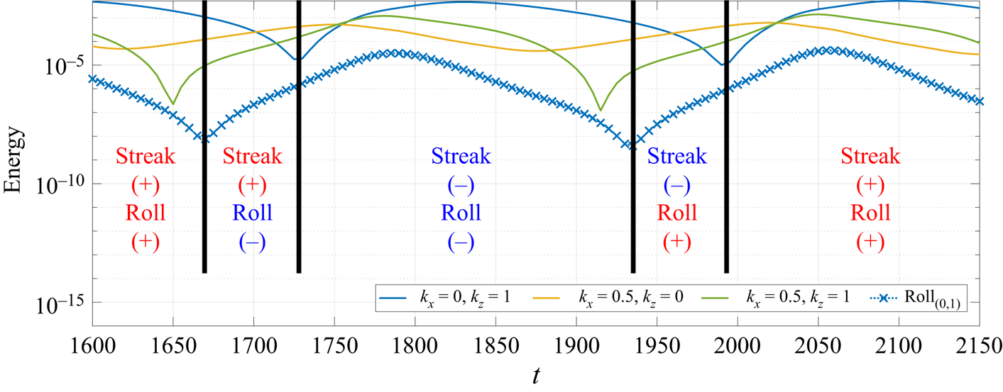
$t=1730$ and $t=1870$: vortices become stable due to high mean-flow distortion, and are exponentially damped in the flow; this is followed by the saturation and decay of oblique waves afterwards. Anti-streaks, generated by anti-rolls, dominate the field, as the correct phase of the lift-up configuration is re-established. Such anti-streaks grow for some time (as a consequence of the lift-up effect) and decay afterwards, as this is a transient growth process (Butler & Farrell Reference Butler and Farrell1992). In this region, the deviation from the laminar solution increases until $t=1800$, which is close to the peak of the streaks, and decays at the subsequent time steps. When the mean-flow distortion is sufficiently small, the instability that generates the vortices is triggered once again. This will restart the half-cycle from $t=1870$, with vortices being generated in the presence of anti-streaks, so that the structures with $k_z \neq 0$ are phase shifted of ${\rm \pi}$ in span in this second part of the cycle. The whole cycle is summarised in figures 15 and 16.


Sketch of the roll–anti-roll dynamics in PAPU flow. Energy of each of the relevant structures in the flow, computed from the DNS. Red fonts (with the  $+$ sign) indicate streaks and rolls, and blue fonts (with the
 $-$ sign) indicate anti-streaks and anti-rolls.

Sketch of the dynamics between coherent structures in PAPU flow. Red fonts indicate streaks and rolls, and blue fonts indicate anti-streaks and anti-rolls. The colour or the circles represent the phase of the streak in that part of the cycle.

Figure 16 displays several similarities to the original diagram of the self-sustained process (SSP) in turbulence for wall-bounded flows, initially proposed by Hamilton et al. (Reference Hamilton, Kim and Waleffe1995). Comparing both diagrams, we observe that streaks and rolls, connected by the lift-up mechanism, remain in the present model, highlighting their role as one of the building blocks of the flow dynamics. However, the ‘ $x$-dependent flow’ in their nomenclature is replaced here by the vortices – which are also streamwise dependent modes, but with distinct characteristics. The main difference is related to the dominant velocity component of the present vortex mode,
 $u$ and
 $v$, in contrast with
 $w$ from the original SSP (Smith, Moehlis & Holmes Reference Smith, Moehlis and Holmes2005; Hall & Sherwin Reference Hall and Sherwin2010; Nogueira et al. Reference Nogueira, Morra, Martini, Cavalieri and Henningson2020). This feature allows a different coupling between vortices and oblique waves, which led to the phase change of the rolls, changing the nature of the cycle. Also, instead of a streak instability generating the
 $x$-dependent flow, as in the SSP, the streamwise variation occurs naturally, due to the presence of an inflection point in the mean flow, which triggers the Kelvin–Helmholtz instability of the vortices. Keeping these differences in mind, the final picture is qualitatively similar to the one drawn by Hamilton et al. (Reference Hamilton, Kim and Waleffe1995), with three coherent structures interacting via stability/lift-up mechanisms, and rolls being regenerated by nonlinear interactions.
5.5. Evidence of the present mechanisms in practical flows
As mentioned in the previous sections, the model presented herein mimics several well-known characteristics of jets and mixing layers, such as jitter (amplitude modulation of vortices) and translational instability. However, considering that turbulence is never achieved in the present numerical simulation, which displays a limit cycle, it becomes necessary to provide more clear-cut connections to the dynamics of practical turbulent shear flows; an example of such connections is provided in this section. Even though the dynamics may seem too simplistic to be representative of interactions in turbulent shear flows, one should keep in mind that many of the key elements observed in turbulent flows are present in this analysis: the well-known axisymmetric Kelvin–Helmholtz wavepacket in jets (Cavalieri et al. Reference Cavalieri, Rodríguez, Jordan, Colonius and Gervais2013; Jordan & Colonius Reference Jordan and Colonius2013) is represented by the vortices  $V$, and its dynamics related to the extraction of energy from the mean flow via an instability mechanism is captured by the model. Streaks and rolls (Nogueira et al. Reference Nogueira, Cavalieri, Jordan and Jaunet2019; Pickering et al. Reference Pickering, Rigas, Nogueira, Cavalieri, Schmidt and Colonius2020), two coherent structures related to each other by the lift-up effect, are also present in the analysis. Nonlinear interactions leading to vortex regeneration, which is known to be one of the important processes in the self-sustained process in turbulence of wall-bounded flows (Hamilton et al. Reference Hamilton, Kim and Waleffe1995; Waleffe Reference Waleffe1997) are modelled here by the interaction between oblique waves
 $O$ and vortices
 $V$.
With all these elements (and their respective physical connections) considered in the cycle, one could use the conclusions of the present analysis to seek such patterns in a turbulent shear flow, and even suggest modifications in the geometry of a nozzle, for instance, in order to achieve desirable effects. Some examples are clearly seen in the literature: it is well known that the inclusion of azimuthal non-uniformity in jet nozzles can lead to the stabilisation of the Kelvin–Helmholtz wavepacket (Sinha et al. Reference Sinha, Gudmundsson, Xia and Colonius2016; Lajús et al. Reference Lajús, Sinha, Cavalieri, Deschamps and Colonius2019), which is related to a reduction in sound radiation and to screech suppression (Samimy, Zaman & Reeder Reference Samimy, Zaman and Reeder1993; Alkislar, Krothapalli & Butler Reference Alkislar, Krothapalli and Butler2007; Zaman, Bridges & Huff Reference Zaman, Bridges and Huff2011). Considering that the addition of tabs and chevrons leads to the formation of rolls (and streaks, consequently), the phenomenon of vortex stabilisation associated to the lift-up stage of the cycle predicted in this model also seems to be present in experimental data. This is an example of how the cycle explored in the previous sections, more clearly depicted in figure 16, provides new elements to analyse/modify turbulent flows.
The same is true for the case of unforced jets and mixing layers, but connections are now given in the context of chaotic attractors in turbulence. Chaotic attractors have properties related to unstable invariant solutions of the dynamical system, and the simplest examples of these are steady or periodic solutions. Trajectories in state space are attracted to such solutions in their stable directions, and subsequently repelled in the unstable directions; see, for instance, Gibson, Halcrow & Cvitanović (Reference Gibson, Halcrow and Cvitanović2009) for an example of how invariant solutions may be used to study complex turbulent dynamics. Such solutions are referred to as exact coherent states (Waleffe Reference Waleffe1998; Kawahara & Kida Reference Kawahara and Kida2001; Wedin & Kerswell Reference Wedin and Kerswell2004; Viswanath Reference Viswanath2007; Cvitanović & Gibson Reference Cvitanović and Gibson2010), and were shown to be an important part in the description of the dynamics of turbulent flows, as solutions often ‘visit’ such states once attracted by the stable directions, leading to coherent patterns. The present cycle is a stable periodic orbit. Ongoing work by our group shows that it loses stability for higher Reynolds numbers, and then becomes an unstable periodic orbit, an exact coherent structure that contributes in shaping turbulence dynamics for free-shear flows. Thus, some parts of this cycle may also be present in turbulent flows.
In order to exemplify that, stereoscopic time-resolved particle image velocimetry from a turbulent jet at Mach  $M=0.4$ was analysed in this framework. The description of the facility and dataset are presented in Cavalieri et al. (Reference Cavalieri, Rodríguez, Jordan, Colonius and Gervais2013), and will not be further detailed here for brevity. Streamwise velocity data was extracted at axial station distant
 $x/D=2$ from the nozzle exit, where
 $D=0.05$ m is the jet diameter. At this position and Mach number, the presence of an axisymmetric wavepacket (azimuthal wavenumber
 $m=0$) was identified; also, as shown in Nogueira et al. (Reference Nogueira, Cavalieri, Jordan and Jaunet2019), streaks associated to azimuthal wavenumber
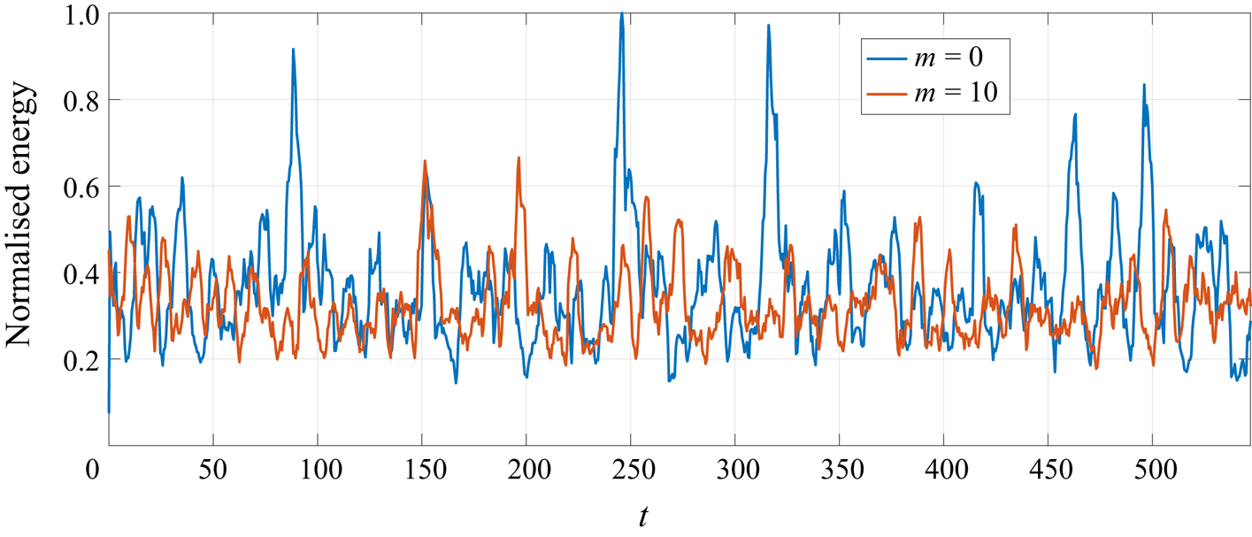
 $m=10$ are expected to be dominant at low frequencies in this jet around the same position, although other wavenumbers are also related to streaks with lower amplitude. The normalised radially integrated energy associated to the aforementioned wavenumbers as a function of time is shown in figure 17, where a simple low-pass temporal filter (moving average with length
 $N=10$) was applied in order to minimise the effect of high-frequency turbulent fluctuations on the signal. The filter will also highlight the presence of streaks and wavepackets in the signal, since both structures are associated to lower frequencies.
Time series of normalised radially integrated energy associated to azimuthal wavenumbers  $m=0$ and
 $m=10$ of a turbulent,
 $M=0.4$, jet at streamwise station
 $x/D=2$. Time
 $t$ is here made non-dimensional using the jet diameter and exit velocity.

Figure 17 displays an overall chaotic behaviour for both values of  $m$, but some correlation between the two signals seems to be present for several time windows. In particular, high peaks of
 $m=0$ wavepacket energy often occur for low
 $m=10$ streak amplitudes. This is consistent with the expectation that a flow should follow coherent dynamics for a limited period of time, in a chaotic attractor, pointing to a mechanism where the presence (absence) of high-
 $m$ streaks could be associated with a stabilisation (destabilisation) of the Kelvin–Helmholtz mode in this turbulent flow, thus leading to times with high or low amplitudes of the
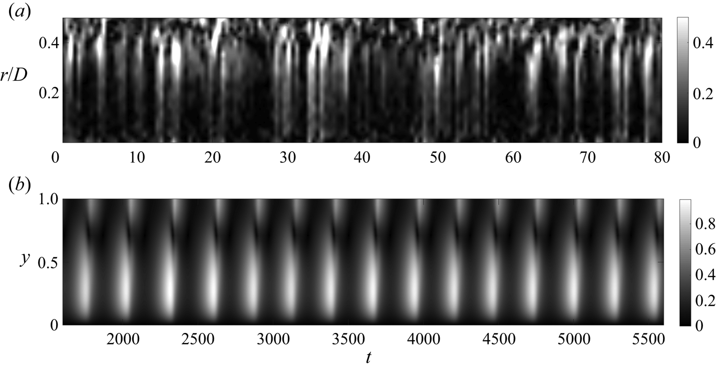
 $m=0$ wavepacket. However, a direct correlation between the time series is not straightforward, since the turbulent jet has streaks with other azimuthal wavenumbers, which are also expected to take part in the dynamics. Further comparison can be drawn by comparing the temporal behaviour of the space–time fields for
 $m=0$ with the vortices in PAPU flow, shown in figure 18. Despite the underlying complexity of the turbulent field compared to the present model, the modulation of the streamwise varying mode is present in both cases, with times of high wavepacket amplitude followed by instants of nearly zero magnitude. The behaviour of the turbulent flow is of course not periodic, but the observed patterns are at times reminiscent of the PAPU-flow cycle illustrated in figure 18(b).
Space-time comparison between the  $m=0$ field of a turbulent jet and the vortices of PAPU flow. In (a)
 $r$ denotes the radial coordinate of the jet. For clarity, only half of the domain is shown in (b). (a) Absolute value of the
 $m=0$ mode in the
 $M=0.4$ turbulent jet. (b) Absolute value of the
 $(0.5,0)$ mode in PAPU flow.

6. Conclusions
The present work introduces and analyses a flow model that includes the most important coherent structures in jets and mixing layers: Kelvin–Helmholtz-like vortices, representing wavepackets in a turbulent jet, and streaks. We start by introducing a toy problem that anticipates most of the observed dynamics in the flow model, a nonlinear, low-order dynamical system, in which all the relevant interactions between coherent structures identified in the paper were explicitly written. The model was designed so as to comply with the rules of triadic interactions between the modes, with the energy transfer between modes written so that the model conserves energy, and displays a limit cycle behaviour with the interplay of all the relevant structures. Kelvin–Helmholtz vortices are seen to grow and decay due to an equivalent mean-flow distortion, related to the other structures. Oblique waves  $O$, rolls
 $R$ and streaks
 $S$ show cyclic behaviour: the growth of oblique waves is coupled to vortices
 $V$ in the stability analysis of a streaky mean flow (2.7) and (2.8), and the sign of
 $O$ depends on the sign of streaks
 $S$; the emergence of oblique waves forces the rolls via (2.4), and forcing depends on the sign of
 $O$; finally, rolls lead to streaks via the lift-up mechanism, manifest in (2.5). In the model, the inversion of sign of any of the quantities,
 $O$,
 $R$ or
 $S$, produces sign inversion of the other ones in successive manner due to the nonlinear interactions in the toy model. This anticipates the dynamics in the flow model analysed in the remaining sections.
To study an actual minimal flow case based on Couette flow, simple enough to allow a detailed analysis of the dynamics, but with the main features of free-shear studies, a permanent actuation in the shape of a hyperbolic tangent is included in the Navier–Stokes equations, generating an inflection point in the base flow that will lead to the exponential growth of vortices at rather low Reynolds numbers. Since the model is based on a sheared flow, streaks also arise as a result of the lift-up mechanism, and these will interact with the vortices via oblique waves. The growth characteristics of these structures are analysed using locally parallel stability and resolvent analyses, and the wavenumbers related to maximum growth were obtained.
A computational box for a direct numerical simulation was designed based on the optimal wavenumbers from stability and resolvent analyses. Results from the simulation display a limit cycle involving streaks, vortices, oblique waves, rolls and the mean flow, as proposed in the toy model, and a clear dynamics between these modes is observed: first, vortices grow exponentially in the flow, followed by the growth of oblique waves in a streaky base flow, with phase anchored by the positions of streaks and vortices. Nonlinear interactions between vortices and oblique waves lead to the generation of anti-rolls in the forcing (streamwise vortices rotating in the opposite direction as the ones found in the velocity field), leading to anti-rolls in the velocity field after some time steps. These generate the opposite streaks (anti-streaks) via lift-up effect, which cancel the former streaks in the flow. The growth of this new energetic structure is associated with the peak deviation of the mean flow from the laminar solution, leading to the saturation and decay of vortices and oblique waves. Afterwards, when all modes are decaying, the deviations from the mean are also diminished, triggering the Kelvin–Helmholtz instability mechanism once again, with vortices in the presence of anti-streaks, which will restart the semi-cycle with a phase shift. The present results show several similarities with the behaviour of jets and mixing layers, reproducing features of Kelvin–Helmholtz jitter (Cavalieri et al. Reference Cavalieri, Jordan, Agarwal and Gervais2011) and keeping some of the characteristics of a translational instability mechanism (Pierrehumbert & Widnall Reference Pierrehumbert and Widnall1982).
The paper is closed with a summary of the self-sustained cycle involving the most important free stream related coherent structures. At this point, it became clear that the dynamical system of five ordinary differential equations, proposed in § 2, managed to reproduce qualitatively most of the dynamics observed in the DNS. Considering the similarities of the present models and the overall behaviour of jets and mixing layers, the simplified models presented here can be useful to understand the turbulent dynamics of such flows, which may lead to insight about engineering solutions that can reduce aircraft noise generation. Jets and mixing layers at high Reynolds numbers display dynamics that are clearly more complex than the limit cycle behaviour explored here, but it is hoped that the interactions between coherent structures, which could be more clearly studied in the present ‘minimal flow’ scenario, may show directions for further probing higher- $Re$ free-shear flows in order to understand and model the complex interactions between wavepackets (Jordan & Colonius Reference Jordan and Colonius2013) and streaks (Nogueira et al. Reference Nogueira, Cavalieri, Jordan and Jaunet2019).
Acknowledgements
P.N. was funded by a CNPq scholarship. A.C. acknowledges financial support by CNPq (grant number 310523/2017-6). We thank Peter Jordan and Eduardo Martini for their comments on the paper, and A. Pinelli for his suggestion of a ‘minimal flow unit’ for the jet. Finally, we thank S. D. Henningson for providing the direct numerical simulation code (SIMSON) and for his support in the Brazil–Sweden collaboration.
Declaration of interests
The authors report no conflict of interest.