





1. Introduction
Due to its important role in the study of buoyancy-driven turbulence, as well as the relevance to free convection occurring in geophysical and astrophysical systems, the simple yet paradigmatic Rayleigh–Bénard convection (RBC) attracts a large number of interests (Siggia Reference Siggia1994; Ahlers, Grossmann & Lohse Reference Ahlers, Grossmann and Lohse2009; Lohse & Xia Reference Lohse and Xia2010; Chilla & Schumacher Reference Chilla and Schumacher2012; Xia Reference Xia2013). In RBC, heat is supplied at the bottom and taken away at the top of the fluid layer. The control parameters of the system are the Rayleigh number  $Ra=\alpha g\,\Delta T\,H^3/\kappa \nu$ representing the magnitude of buoyancy-driven force, the Prandtl number
 $Pr=\nu / \kappa$ describing the fluid properties, and the aspect ratio of the convection cell
 $\varGamma =D/H$. Here,
 $g$ is the gravitational acceleration,
 $H$ and
 $D$ are the height and diameter of the upright cylindrical convection cell,
 $\Delta T$ is the temperature difference across the fluid layer, and
 $\alpha$,
 $\kappa$ and
 $\nu$ are respectively the thermal expansion coefficient, thermal diffusivity and kinematic viscosity of the working fluid.
A fascinating feature of RBC is the existence of the large-scale circulation (LSC) (or vortex) that spans the size of the convection cell (Krishnamurti & Howard Reference Krishnamurti and Howard1981; Castaing et al. Reference Castaing, Gnuaratne, Heslot, Kadanoff, Libchaber, Thomae, Wu, Zaleski and Zanetti1989; Xi, Lam & Xia Reference Xi, Lam and Xia2004; Zhu et al. Reference Zhu, Jiang, Zhou and Sun2019). The LSC, which originates from the self-organization of the thermal plumes that stem from both top and bottom boundary layers, is of great importance because it controls the heat and momentum transfer of the system. Most of the previous studies of the LSC focused on the  $\varGamma = 1$ cylindrical cell due to its simplicity in cell geometry. The LSC (the quasi-two-dimensional vertical structure) has been investigated extensively for its copious flow dynamics, such as the azimuthal motion (Brown, Nikolaenko & Ahlers Reference Brown, Nikolaenko and Ahlers2005; Xi, Zhou & Xia Reference Xi, Zhou and Xia2006), cessation (Brown et al. Reference Brown, Nikolaenko and Ahlers2005; Xi & Xia Reference Xi and Xia2008), reversal (Niemela et al. Reference Niemela, Skrbek, Sreenivasan and Donnelly2001; Xi & Xia Reference Xi and Xia2007, Reference Xi and Xia2008; Sugiyama et al. Reference Sugiyama, Ni, Stevens, Chan, Zhou, Xi, Sun, Grossmann, Xia and Lohse2010; Verma & Mahendra Reference Verma and Mahendra2013; Ni, Huang & Xia Reference Ni, Huang and Xia2015; Wang et al. Reference Wang, Lai, Song and Tong2018; Castillo-Castellanos et al. Reference Castillo-Castellanos, Podvin, Sergentand and Rossi2019; Chen et al. Reference Chen, Huang, Xia and Xi2019; Chen, Wang & Xi Reference Chen, Wang and Xi2020; Xu, Chen & Xi Reference Xu, Chen and Xi2021), torsional (Funfschilling & Ahlers Reference Funfschilling and Ahlers2004; Funfschilling, Brown & Guenter Reference Funfschilling, Brown and Guenter2008; Xi & Xia Reference Xi and Xia2008; Zhou et al. Reference Zhou, Xi, Zhou, Sun and Xia2009) and sloshing motions (Xi et al. Reference Xi, Zhou, Zhou, Chan and Xia2009; Zhou et al. Reference Zhou, Xi, Zhou, Sun and Xia2009; Brown & Ahlers Reference Brown and Ahlers2009; Zürner et al. Reference Zürner, Schindler, Vogt, Eckert and Schumacher2019; Zwirner et al. Reference Zwirner, Khalilov, Kolesnichenko, Mamykin, Mandrykin, Pavlinov, Shestakov, Teimurazov, Frick and Shishkina2019). However, ubiquitous convections occurring in nature are of larger aspect ratio, such as convection in the mantle and outer core of the Earth, in the atmosphere, in the ocean and in the Sun. And it is still unclear whether the conclusions drawn from the small aspect ratio convection can be extended directly to the more frequently occurring larger aspect ratio cases. In addition, previous findings indicated that the large-scale flow structure would go through a transition from the single-roll form to the multi-roll form around the aspect ratio
 $\varGamma =2$, which motivates us to explore this interesting coherent structure that is directly related to the heat and momentum transfer in this special geometry regime (Naert, Segawa & Sano Reference Naert, Segawa and Sano1997; Qiu & Tong Reference Qiu and Tong2001a; Qiu et al. Reference Qiu, Shang, Tong and Xia2004; Funfschilling et al. Reference Funfschilling, Brown, Nikolaenko and Ahlers2005; Sun et al. Reference Sun, Ren, Song and Xia2005a; Tsuji et al. Reference Tsuji, Mizuno, Mashiko and Sano2005; du Puits, Resagk & Thess Reference du Puits, Resagk and Thess2007; Xia, Sun & Cheung Reference Xia, Sun and Cheung2008; Bailon-Cuba, Emran & Schumacher Reference Bailon-Cuba, Emran and Schumacher2010; Vogt et al. Reference Vogt, Horn, Grannan and Aurnou2018).
Previous experiments with local velocity measurements through laser Doppler velocimetry (LDV) (Qiu & Tong Reference Qiu and Tong2001a) reveal that the flow in the  $\varGamma = 2$ cylindrical cell is in the single-roll form. And this result is confirmed by later experiments and numerical simulations (Sun et al. Reference Sun, Ren, Song and Xia2005a; Bailon-Cuba et al. Reference Bailon-Cuba, Emran and Schumacher2010), while a later study with LDV local velocity measurements shows that the single-roll structure breaks down into two side-by-side rolls when
 $\varGamma$ is increased to
 $1.68$ (du Puits et al. Reference du Puits, Resagk and Thess2007). Recently, a study combining the numerical simulation and local velocity measurements (through an ultrasonic Doppler technique) in low-
 $Pr$ fluid (liquid gallium) proposes that the flow takes a very different form, called the ‘jump rope’ mode (Vogt et al. Reference Vogt, Horn, Grannan and Aurnou2018). Their simulation results further suggested that the newly observed ‘jump rope’ motion also exists at moderate
 $Pr$ such as in water, but with a much weaker signal. To make a decisive conclusion on whether the LSC in
 $\varGamma = 2$ cells takes the form of a quasi-two-dimensional single-roll form or the so-called ‘jump rope’, or already breaks down, a direct measurement of the three-dimensional flow structure in the
 $\varGamma =2$ cylindrical cell is crucial.
In this work, we systematically investigate the dynamics of the three-dimensional structure of the large-scale flow in a  $\varGamma = 2$ cylindrical cell by measuring the velocity field in different vertical cross-sectional planes using the particle image velocimetry (PIV) technique. The rest of this paper is organized as follows. In § 2, we describe the experimental conditions. In § 3, we present the flow structures measured in different vertical planes, and analyse the orbiting of the vortex centre, followed by a discussion on the velocity oscillations at the centre of the cell. In § 4, we summarize the main findings of this work.
2. Experimental set-up
The convection cell is similar to those used in previous experiments (Xi et al. Reference Xi, Zhang, Hao and Xia2016). It is an upright cylindrical cell with inner diameter  $D = 190$ mm and height
 $H = 95$ mm, so the aspect ratio is
 $\varGamma = D/H \simeq 2$. Both the top and bottom plates are made of copper of thickness
 $3.5$ cm, and the side wall is a Plexiglas cylinder of thickness
 $0.5$ cm. A refrigerated circulator (PolyScience, PP15R-40-A12Y) is used to adjust the temperature at the top plate. The resistive film heaters heat the bottom plate with constant power input. The temperatures of the top and bottom plates are measured by nine thermistors (Omega 44031) of diameter 2.5 mm embedded in the plates, and they are nearly 2 mm away from the fluid–solid interface. Four of them are evenly distributed azimuthally in 90
 $^\circ$ intervals and embedded in the half-radius from the centre of the plate in the top/bottom plate. In the bottom plate, there is an extra thermistor that is embedded at the centre of the plate.
To reduce the distortion effect on the PIV images caused by the curvature of the side wall of the cylindrical cell, a rectangular-shaped jacket made of 3 mm thick Plexiglas plates is glued to the outside of the cylindrical cell and is filled with deionized water. Because of the presence of the jacket, the measured area is slightly smaller than the cell in the vertical direction (80 mm, versus the actual height of the cell, 95 mm), thus the region near the boundary layer cannot be detected in the PIV measurement.
Deionized water is used as the working fluid, and during the whole experiment we keep the mean bulk temperature at  $\bar {T} = 28^\circ$C. The corresponding thermal expansion coefficient
 $\alpha$, kinematic viscosity
 $\nu$, and thermal diffusivity
 $\kappa$ of water are, respectively,
 $2.85\times 10^{-4}$ K
 $^{-1}$,
 $8.36\times 10^{-7}$ m
 $^2$s
 $^{-1}$ and
 $1.47\times 10^{-7}$ m
 $^2$s
 $^{-1}$. Here,
 $\bar {T} =( T_{top}+T_{bottom})/2$ and
 $T_{top}$ (
 $T_{bottom}$) is the temperature of the top (bottom) plate, with corresponding Prandtl number
 $Pr \approx 5.7$. The Rayleigh number varies in the range
 $7.64 \times 10^7 \leq Ra \leq 6.06 \times 10^8$, hence covering almost an order of magnitude. During the experiments, the cell is tilted by
 $2^\circ$ (as shown in figure 1), thus the central LSC plane (
 $d_{\parallel }=0$ plane) is locked in the vertical axial plane containing the position where the cell is tilted. The velocity fields in the five vertical cross-sections of the cell are measured by the planar PIV system (Dantec Dynamics); three of them are in or parallel to the LSC central plane (i.e.
 $d_{\parallel }=0$,
 $d_{\parallel } = 0.5r$ and
 $d_{\parallel } = 0.95r$), and the other two are perpendicular to the LSC central plane (i.e.
 $d_\perp =0$ and
 $d_\perp =2r/3$), as shown in figure 1. Here,
 $d_{\parallel }$ and
 $d_\perp$ are the distances to the vertical axis of the cylindrical cell. The PIV velocity measurements in the LSC central plane (
 $d_{\parallel }=0$) were performed at six
 $Ra$ (
 $7.64 \times 10^7$,
 $1.55 \times 10^8$,
 $3.17 \times 10^8$,
 $4.45 \times 10^8$,
 $4.97\times 10^8$ and
 $6.06 \times 10^8$), while in the other planes the velocity measurements were performed at three
 $Ra$ (
 $7.64 \times 10^7$,
 $3.17 \times 10^8$ and
 $6.06 \times 10^8$). The obtained results are qualitatively the same for different
 $Ra$, thus, unless stated otherwise, only those for
 $Ra=6.06 \times 10^8$ are presented below.
Sketch of the convection cell and the five planes where the planar PIV velocity measurements are conducted. The cell is tilted by 2 $^\circ$, and
 $d_{\parallel }=0$ is the central plane of the LSC. The planar PIV velocity measurements were conducted in the
 $d_{\parallel }=0$ plane and two planes (
 $d_{\parallel } = 0.5r$ and
 $d_{\parallel } = 0.95r$) in parallel to the
 $d_{\parallel }=0$ plane, and two planes (
 $d_\perp =0$ and
 $d_\perp =2r/3$) perpendicular to the
 $d_{\parallel }=0$ plane.

3. Results and discussion
3.1. Mean velocity field
We first show the flow fields measured by the planar PIV in the planes parallel to the LSC central plane. In each plane, the measurement lasts for at least two hours (corresponding to 42–110 orbiting periods of the vortex centre for different  $Ra$ – see § 3.2 for details) such that at least 7200 velocity maps were acquired with the sampling rate of 1 Hz. Figure 2 shows the long-time-averaged velocity map measured in the three vertical planes that are in or parallel to the LSC central plane at
 $Ra=6.06\times 10^8$. From figure 2(a), we can see that the flow in the LSC central plane (
 $d_{\parallel }=0$) is in the single-roll form with its horizontal size being two times its vertical size, and no prominent corner rolls are observed. From the magnitude of the velocity in figure 2(a), we can see that the maximum velocity appears near the top and bottom plates, which is consistent with previous measurements by LDV (Qiu & Tong Reference Qiu and Tong2001a). And this is different from the case in the
 $\varGamma = 1$ cells where the largest velocity appears near the mid-height of the vertical side wall (Sun, Xia & Tong Reference Sun, Xia and Tong2005b). The reason is that in the
 $\varGamma = 2$ cells, the horizontal flow near the conducting surfaces takes up less space than the vertical flow near the side wall; according to mass conservation, the horizontal and vertical flows must carry the same amount of fluid, as the horizontal flow near the conducting surfaces takes up less space, the flow velocity must be larger.
Long-time-averaged PIV velocity map in the three parallel vertical planes: (a)  $d_{\parallel } = 0$, (b)
 $d_{\parallel } = 0.5r$, and (c)
 $d_{\parallel } = 0.95r$, at
 $Ra = 6.06 \times 10^8$. The magnitude of the velocity
 $\sqrt {U^2+W^2}$ is coded in both the colour of the map and the lengths of the arrows, in units of cm s
 $^{-1}$. The time average is performed over a period of two hours, corresponding to 110 times the period of the orbiting of the vortex centre.

Figures 2(b) and 2(c) present the averaged velocity field in the  $d_{\parallel } = 0.5r$ plane and the
 $d_{\parallel } = 0.95r$ plane, respectively. It is found that in those two planes that are far away from the cell centre, the flow is still in the form of a single roll, which implies that the width of the LSC band is at least
 $0.95D$. This is very different from the case in the
 $\varGamma = 1$ cells where the width of the LSC is about half of the diameter of the convection cell (Lui & Xia Reference Lui and Xia1998; Sun et al. Reference Sun, Xia and Tong2005b; Xi & Xia Reference Xi and Xia2008). Although the flow patterns in the three planes are very similar to each other, the magnitude of the velocity gradually decreases when it is farther away from the cell vertical axis. Another feature that we observed is that the long axis of the ellipse-shaped large-scale structure is along the horizontal direction in the
 $d_{\parallel } = 0$ and
 $d_{\parallel } = 0.5r$ planes (figures 2a and 2b), while in the
 $d_{\parallel } = 0.95r$ plane the ellipse-shaped single-roll structure is slightly tilted, which may be due to the confinement of the side wall in this plane.
We noticed that there is a slight up–down asymmetry of the flow strength in the long-time-averaged flow field as shown in figures 2(a) and 2(b). We would attribute this asymmetry to the imperfections in experiments. Two possible factors account for the imperfections. First, as we mentioned in § 2, in order to reduce the distortion caused by the curvature of the side wall, we have to use a rectangular-shaped jacket whose height is smaller than the height of the cell (80 mm versus 95 mm). Due to the existence of the jacket, there are small regions near the end plates that cannot be measured by the PIV. Besides, the possible slight misalignment of the camera to the region of measurement could also introduce the asymmetry shown in the velocity field. Despite the slight asymmetry, we believe that it does not affect the conclusions of this paper.
3.2. Orbiting of the vortex centre
Although the long-time-averaged velocity fields in the planes parallel to the LSC central plane are in the single-roll form with the vortex centre at the centre of the plane, the instantaneous velocity fields show that the centre of the LSC actually undergoes periodical orbiting around the centre of the plane, and the direction of the orbiting is opposite to the flow direction of the LSC. The periodical orbiting can be seen clearly from the time trace of the position ( $X_0, Z_0$) of the vortex centre shown in figure 3(a), where both the
 $x$ and
 $z$ coordinates of the vortex centre exhibit very clear periodicity. Here the position of the vortex centre is identified manually from the instantaneous PIV velocity map. While in the
 $d_{\parallel } = 0.5r$ plane, the periodicity of the position of the vortex centre is not visible and in this plane the motion of the vortex centre is confined in a smaller range, as shown in figure 3(b). And when we examine the time trace of the vortex centre in the
 $d_{\parallel } = 0.95r$ plane, the periodicity appears again as shown in figure 3(c). To compare the current results in
 $\varGamma = 2$ cells with those in
 $\varGamma =1$ cells, we also performed PIV measurements in the
 $d_{||} = 0$ plane in a
 $\varGamma =1$ cell and find that the time trace of the position of the vortex centre does not show appreciable periodicity; in addition, the motion of the vortex centre is confined in a very small area as shown in figure 3(d) (the r.m.s. values of the position of the vortex centre are
 $1.49$ cm in the
 $x$ direction and
 $1.66$ cm in
 $z$ direction, compared to the values
 $3.92$ cm,
 $2.17$ cm in the
 $d_{||} = 0$ plane in
 $\varGamma =2$ cells).
Time trace of the position of the vortex centre measured in the three parallel vertical planes: (a)  $d_{\parallel } = 0$, (b)
 $d_{\parallel } = 0.5r$, and (c)
 $d_{\parallel } = 0.95r$, at
 $Ra = 6.06 \times 10^8$ in the
 $\varGamma =2$ cell. For comparison, (d) shows the time trace of the position of the vortex centre in the
 $d_{\parallel } = 0$ plane in the
 $\varGamma =1$ cell at
 $Ra = 5.25 \times 10^9$.

The periodicity of the orbiting of the vortex centre in the  $d_{\parallel } = 0$ and
 $d_{\parallel } = 0.95r$ planes is also evidenced statistically by the autocorrelation of the position of the vortex centre in the
 $x$ and
 $z$ directions, as shown in figures 4(a) and 4(c). The autocorrelation of the position of the vortex centre in the
 $d_{\parallel } = 0.5r$ plane shows very weak periodicity (figure 4b), and the autocorrelation of the position of the vortex centre in the
 $d_{\parallel } = 0$ plane in
 $\varGamma =1$ cells shows almost no periodicity (figure 4d), which are consistent with the time traces shown in figure 3. In figure 4(e), we show the period of the vortex centre orbiting
 $\tau$ as a function of
 $Ra$; with
 $\tau = 776247.12\,Ra^{-0.46\pm 0.01}$, the scaling exponent is in agreement with that of the turnover time of the LSC obtained from the autocorrelation/cross-correlation of the temperature signals in previous studies (Sun & Xia Reference Sun and Xia2005). We also defined a Reynolds number
 $Re=H^2/(\tau \kappa )$ (or
 $Re=H^2f_0/\kappa$, where
 $f_0=1/\tau$) based on the period of the vortex centre orbiting
 $\tau$. It is found that
 $Re$ increases with
 $Ra$ as
 $Re\,Pr=0.08\,Ra^{0.46}$, as shown in figure 4( f). The scaling exponent obtained in our experiments agrees well with the previous results obtained also at moderate
 $Pr$ (in water) where the Reynolds number is based on the oscillation frequency of the local velocity (Qiu & Tong Reference Qiu and Tong2001b; Qiu et al. Reference Qiu, Shang, Tong and Xia2004), while compared to the results at smaller
 $Pr$ (
 $Pr\approx 0.027$ in liquid gallium, and the Reynolds number is also obtained from the oscillation frequency of the local velocity),
 $Re\,Pr=0.027\,Ra^{0.419}$ (Vogt et al. Reference Vogt, Horn, Grannan and Aurnou2018), our scaling exponent is slightly larger.
Autocorrelation of the time trace of the position of the vortex centre measured in the three parallel vertical planes: (a)  $d_{\parallel } = 0$, (b)
 $d_{\parallel } = 0.5r$, and (c)
 $d_{\parallel } = 0.95r$, at
 $Ra = 6.06 \times 10^8$ in the
 $\varGamma =2$ cell. For comparison, the autocorrelation of the time trace of the position of the vortex centre in the
 $d_{\parallel } = 0$ plane in the
 $\varGamma =1$ cell at
 $Ra = 5.25 \times 10^9$ is also plotted in (d). Panels (e) and ( f) show the period of the orbiting of the vortex centre
 $\tau$ and the Reynolds number based on
 $\tau$ (
 $Re=H^2/(\tau \kappa )$), as functions of
 $Ra$.

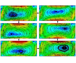
To better present the periodical orbiting of the vortex centre, we show in figure 5 the phase-averaged PIV velocity maps at phases  $t_0$,
 $t_0+\tau /6$,
 $t_0+\tau /3$,
 $t_0+\tau /2$,
 $t_0+2\tau /3$ and
 $t_0+5\tau /6$, at
 $Ra = 6.06 \times 10^8$. The corresponding movie can be viewed as supplementary movie 1, available at https://doi.org/10.1017/jfm.2022.11. Here
 $\tau$ is the period of the orbiting of the vortex centre as is indicated in figure 4. The phase average is calculated as follows. Suppose that in one period of the vortex centre orbiting we have captured
 $m$ velocity maps. We then take the average of the velocity maps numbered
 $1,m+1,2m+1,3m+1,\ldots$ as the phase-averaged velocity map at
 $t_0$, and similarly, the average of the velocity maps numbered
 $2,m+2,2m+2,3m+2,\ldots$ as the phase-averaged velocity map at
 $t_0+\tau /m$; in this way, the phase-averaged velocity maps in the whole period are obtained. It is seen from the figure that the centre of the big vortex is located on the left of the plane at phase
 $t=t_0$ (figure 5a); after approximately
 $\tau$/6, it moves to the lower left of the plane (figure 5b); it keeps going and arrives at the lower middle of the plane at
 $t_0+\tau /3$ (figure 5c); the vortex centre then goes to the middle right of the plane (figure 5d), then the upper right of the plane (figure 5e), then the upper middle of the plane (figure 5f); and finally it goes back to the position where it was at
 $t=t_0$. Clearly, the centre of the vortex moves in the counter-clockwise direction, which is opposite to the flow direction of the LSC.
Phase-averaged PIV velocity maps measured in the central vertical plane of the convection cell ( $d_{\parallel }=0$) at phases
 $t_0$,
 $t_0+\tau /6$,
 $t_0+\tau /3$,
 $t_0+\tau /2$,
 $t_0+2\tau /3$,
 $t_0+5\tau /6$, respectively, for
 $Ra = 6.06 \times 10^8$. The magnitude of the velocity
 $\sqrt {U^2+W^2}$ is coded in both colour and the lengths of the arrows (units of cm s
 $^{-1}$). The value
 $t_0$ is the starting time of a new period, and
 $\tau$ is the period of the orbiting of the vortex centre. The dashed lines denoted by ‘A’ and ‘B’ (in a and d) show the two planes perpendicular to
 $d_{\parallel }=0$, namely
 $d_\perp = 0$ and
 $d_\perp = 2r/3$, where the PIV measurements are also conducted. The cell is tilted by
 $2^\circ$ at the left, as shown in the figure.

In order to study quantitatively the orbiting of the vortex centre, we manually identified the centre of the vortex from the phase-averaged PIV velocity maps, and obtained the trajectories of the vortex centre in the  $d_{\parallel } = 0$,
 $d_{\parallel } = 0.5r$ and
 $d_{\parallel } = 0.95r$ planes. Figure 6 shows the trajectory of the vortex centre measured in the three planes for
 $Ra = 6.06 \times 10^8$. In the figure, the arrows show the direction of the vortex centre motion, and the colour represents the phase of the trajectory. In the
 $d_{\parallel } = 0$ plane, where the measured section is the largest, the vortex centre orbits within a large ellipse loop, as shown by the coloured elliptical trajectory. In the
 $d_{\parallel }=0.5r$ plane, the trajectory is confined in a much smaller ellipse as shown in figure 6(b). In the
 $d_{\parallel } = 0.95r$ plane, it is found that the vortex centre orbits within an ellipse loop that is similar to the case in the
 $d_{\parallel } = 0$ plane, but the size of the ellipse is smaller than that in the
 $d_{\parallel } = 0$ plane. We can also see from the figure that the motion of the vortex centre is in the counter-clockwise direction, which is opposite to the flow direction of the LSC. And the direction of the motion of the vortex centre is the same in all the three planes that we have measured.
Trajectory of the vortex centre in the three parallel vertical planes: (a)  $d_{\parallel } = 0$, (b)
 $d_{\parallel } = 0.5r$, and (c)
 $d_{\parallel } = 0.95r$, at
 $Ra = 6.06 \times 10^8$ in the
 $\varGamma =2$ cell. And (d) shows the trajectory of the vortex centre in the
 $d_{\parallel } = 0$ plane in the
 $\varGamma =1$ cell at
 $Ra = 5.25 \times 10^9$. The dashed lines in (b) and (c) show the side wall. The arrows show the direction of the vortex centre motion, and the colour represents the phase of the trajectory.

Taking all the measurements in the three planes, we come to the conclusion that the centre of the large-scale circulation (or the big vortex) is not fixed at the plane centre; rather, it orbits periodically around the plane centre. In the  $d_{\parallel }=0$ plane (the plane containing the vertical axis of the cell), the radius of the orbit of the vortex centre is largest; when it is away from the vertical axis of the cell, the radius of the orbit decreases, and reaches a minimum around
 $d_{\parallel }=0.5r$; then the radius of the orbit increases when it gets further away from the vertical axis of the cell. The decrease and increase of the magnitude of the orbiting of the vortex centre reveals that the LSC is not a two-dimensional narrow band, its thickness is as large as the size of the cell diameter. The central part of the LSC forms a vortex tube, and the centre line of the vortex tube is curved rather than straight. Previously, it was found that the large-scale circulation contains a ‘jump rope’ mode (Vogt et al. Reference Vogt, Horn, Grannan and Aurnou2018); now with the planar PIV measurements in the three parallel planes, it is clear that the so-called ‘jump rope’ mode actually is the orbiting of the centre line of the vortex tube, and the magnitude of the orbiting is largest near the centre of the convection cell, decreases, and then increases along the radius. The minimum orbiting radius implies that the axis of rotation of the ‘jump rope’ is roughly at the centre of the
 $d_{\parallel } = 0.5r$ plane. Previously, combining both the multi-point ultrasonic velocity measurements and numerical simulation, Vogt et al. (Reference Vogt, Horn, Grannan and Aurnou2018) showed that the ‘jump rope’ exists in the low-
 $Pr$ convection in the cell with aspect ratio
 $\sqrt {2}<\varGamma <2$. Here in RBC at moderate
 $Pr$, the two-dimensional velocity measurements in different planes enable us to reconstruct the three-dimensional flow structure, and directly show that the essence of the ‘jump rope’ mode is the orbiting of the vortex centre.
To see whether this orbiting of the vortex centre also exists in the  $\varGamma =1$ cylindrical cell, we also performed planar PIV velocity measurements in a
 $\varGamma =1$ cell. It is found that for the
 $\varGamma =1$ cell in the
 $d_{\parallel }=0$ plane, the position of the vortex centre is concentrated at the centre of the plane, which implies that the vortex centre stays at the centre of the plane, without any orbiting. This is confirmed by the random and low magnitude of the trajectory of the vortex centre obtained by the phase-averaged velocity maps shown in figure 6(d). The non-periodicity and very small amplitude of the motion of the vortex centre imply that the periodical orbiting of the vortex centre does not exist in
 $\varGamma =1$ cells, at least at the
 $Ra$ of our experiment (
 $Ra = 5.25\times 10^9$). It is very likely the case that the periodical orbiting of the vortex centre does not exist in the
 $\varGamma =1$ cell at other
 $Ra$, as it was not reported in the vast amounts of literature about the LSC in the
 $\varGamma =1$ cell. The reason why the orbiting of vortex centre exists only in
 $\varGamma =2$ cells but not in
 $\varGamma =1$ cells is not known to us. One speculation is that the interaction between the plumes erupting from the top/bottom plate with this specific cell height (
 $\varGamma$) meets the criteria for stable periodical orbiting to occur.
3.3. Flow field in the planes perpendicular to the LSC
We then explore the flow field in the two planes perpendicular to the LSC central plane, namely  $d_\perp = 0$ and
 $d_\perp = 2r/3$, where
 $0$ and
 $2r/3$ are the distances to the vertical axis of the cell. The two planes are also marked by ‘B’ and ‘A’ in figures 5(a) and 5(d). Figures 7(a) and 7(b) show the phase-averaged PIV velocity maps measured in the
 $d_\perp = 0$ plane for
 $Ra = 6.06 \times 10^8$ at
 $t=t_0$ and
 $t=t_0+\tau /2$. It is found that it contains a pair of side-by-side vortices with opposite rotating directions. And these two vortices reverse their rotating directions periodically with the period
 $\tau$, which is the same as the period of the orbiting of the centre of the LSC. At
 $t=t_0$, the left vortex is rotating in the clockwise direction and the right one is rotating in the counter clockwise direction, thus the fluid at the middle descends and the fluid on both sides ascends (figure 7a); after
 $\tau /2$, the rotating directions of the two vortices reverse, and as a result the fluid at the middle ascends and the fluid on both sides descends (figure 7b). This periodical reversal of the flow direction of the two vortices is actually caused by the periodical orbiting of the centre of the LSC, as evidenced in figures 5(a) and 5(d). One can see that: at
 $t=t_0$ the centre of the vortex moves to the left-hand side of the cell, at the centre of the cell along the vertical line marked by ‘B‘ the flow is descending; and when it comes to
 $t=t_0+\tau /2$, the centre of the vortex moves to the right-hand side of the cell, and the flow becomes ascending along the line marked by ‘B’.
Phase-averaged velocity field in the planes perpendicular to the LSC central plane at  $Ra \!=\! 6.06 \!\times\! 10^8$: (a,b) in the
 $d_\perp = 0$ plane at
 $t=t_0$ and
 $t=t_0+\tau /2$, respectively; (c,d) in the
 $d_\perp = 2r/3$ plane at
 $t=t_0$ and
 $t=t_0+\tau /2$, respectively. The magnitude of the vertical component (
 $W$) or the horizontal component (
 $V$) of the velocity in the plane is coded by colour, in units of cm s
 $^{-1}$. The lengths of the arrows represent the magnitudes of velocity
 $\sqrt {V^2+W^2}$.

Previously in the convection of low- $Pr$ fluid (liquid metal) in a
 $\varGamma =2$ cell, Vogt et al. (Reference Vogt, Horn, Grannan and Aurnou2018) made velocity measurements along a chord in the mid-height horizontal plane and
 $2r/3$ away from the vertical axis of the cell by using ultrasonic Doppler velocimetry (UDV). It is found that along this line, the fluid is periodically changing from diverging from the LSC central plane and then converging back towards it. To make a quantitative comparison with these results, we made a PIV velocity measurement in our system in the
 $d_\perp = 2r/3$ plane, denoted by ‘A’ in figures 5(a) and 5(d). It is seen that the flow diverges to both sides from the middle of the plane at
 $t=t_0$ (figure 7c); after
 $\tau /2$, the flow converges to the middle of the plane from both sides of the plane (figure 7d). Note that the middle line of the
 $d_\perp = 2r/3$ plane is also in the LSC central plane (
 $d_{\parallel }=0$ plane). Thus the divergence and then convergence of the flow are consistent with the results in the low-
 $Pr$ fluid (Vogt et al. Reference Vogt, Horn, Grannan and Aurnou2018). The periodical diverging and converging flow measured here actually originates from the periodical orbiting of the vortex centre. When the vortex centre moves from the top right corner to the bottom left corner, as shown in figures 5(e), 5( f) and 5(a), the ascending fluid on the left of the cell is pushed to the left and spread, resulting in the diverging flow field observed from the PIV velocity map shown in figure 7(c). On the other hand, when the vortex centre moves from the bottom left corner to the top right corner as shown in figure 5(b–e), the ascending fluid on the left of the cell is pulled to the right, resulting in the converging flow field observed from the PIV velocity map shown in figure 7(d).
To compare the flow strength parallel and perpendicular to the LSC central plane, we plotted in figure 8 the phase-averaged PIV velocity map in the three parallel vertical planes where the magnitude of vertical component ( $W$) of the velocity in the plane is coded by colour. As shown in figure 8, in the
 $d_{\parallel }=0$,
 $d_{\parallel }=0.5r$ and
 $d_{\parallel }=0.95r$ planes, the maximum velocities (the
 $W$ component) of the phase-averaged velocity fields are approximately
 $0.8$ cm s
 $^{-1}$,
 $0.8$ cm s
 $^{-1}$ and
 $0.7$ cm s
 $^{-1}$, which are much larger than that in the
 $d_\perp = 0$ plane, where the maximum velocity (the
 $W$ component) is about
 $0.5$ cm s
 $^{-1}$ (as shown in figure 7). Our study shows clearly that the flow in the planes parallel to the LSC central plane dominates over that in the planes perpendicular to the LSC central plane.
Phase-averaged velocity field in the planes parallel to the LSC central plane at  $Ra = 6.06 \times 10^8$: (a,b) in the
 $d_\parallel = 0$ plane at
 $t=t_0$ and
 $t=t_0+\tau /2$, respectively; (c,d) in the
 $d_\parallel = 0.5r$ plane at
 $t=t_0$ and
 $t=t_0+\tau /2$, respectively; (e,f) in the
 $d_\parallel = 0.95r$ plane at
 $t=t_0$ and
 $t=t_0+\tau /2$, respectively. The magnitude of the vertical component (
 $W$) of the velocity in the plane is coded by colour, in units of cm s
 $^{-1}$. The lengths of the arrows represent the magnitudes of velocity
 $\sqrt {U^2+W^2}$.

3.4. The oscillation of the local velocity
The orbiting of the vortex centre is also evidenced by the variation of the local velocity at the centre of the  $d_{\parallel } = 0$ and
 $d_{\parallel } = 0.95r$ planes. Figure 9 shows the probability density functions (PDFs) of the normalized horizontal and vertical velocities at the centre of the
 $d_{\parallel } = 0$,
 $d_{\parallel } = 0.5r$ and
 $d_{\parallel } = 0.95r$ planes. It is seen that the PDF of the horizontal component of velocity
 $u$ at the centre of the
 $d_{\parallel } = 0$ plane (figure 9a) shows two peaks; one peak is positive and the other is negative, which means that there are two probable flow direction at the plane centre, one is pointing to the left and the other is pointing to the right. This double-peak distribution of
 $u$ is due to the motion of the vortex centre: when the vortex centre is above the mid-height plane of cell, the direction of horizontal velocity at the plane centre is pointing to the left; when the vortex centre is below the mid-height plane of cell, the direction of horizontal velocity at the plane centre is pointing to the right. This left-pointing and right-pointing horizontal velocity at the centre appears periodically and alternately due to the periodical orbiting of the centre of the vortex, thus
 $u$ shows the double-peak distribution. Similarly, when the vortex centre is at the left of cell centre, the direction of vertical velocity at the plane centre is pointing up; when the vortex centre is at the right of the cell centre, the direction of vertical velocity at the plane centre is pointing down. This up-pointing and down-pointing vertical velocity at the centre appears periodically and alternately due to the periodical orbiting of the centre of the vortex, thus
 $w$ shows the double-peak distribution, as shown in figure 9(b). Despite the similar form, the double peak is clearer in the PDF of
 $u$, as in the
 $\varGamma =2$ cell the horizontal velocity dominates the vertical counterpart. The PDFs of
 $u$ and
 $w$ measured at the centre of the
 $d_{\parallel } = 0.95r$ plane (figures 9e and 9f) are similar to those in the
 $d_{\parallel } = 0$ plane. On the other hand, the PDFs of
 $u$ and
 $w$ measured at the centre of the
 $d_{\parallel }$= 0.5r plane do not show an appreciable double-peak feature (figure 9c), which is consistent with the fact that the motion of the vortex centre in the
 $d_{\parallel } = 0.5r$ plane is confined in a much smaller range, and the ‘supporting point’ of the ‘jump rope’ motion is around the centre of the
 $d_{\parallel } = 0.5r$ plane.
The probability density functions (PDFs) of velocity components  $u$ and
 $w$ at the centre of (a,b) the
 $d_{\parallel } = 0$ plane, (c,d) the
 $d_{\parallel } = 0.5r$ plane, and (e,f) the
 $d_{\parallel } = 0.95r$ plane, for
 $\varGamma =2$. Here,
 $\mu _i$ and
 $\sigma _i$ (where
 $i$ is
 $u$ or
 $w$) respectively denote the mean and standard deviation of the velocity component.

The periodicity of the orbiting of the vortex centre is also evidenced by the prominent peaks in the power spectra of the local velocity components  $u$ and
 $w$ measured at the centre of the
 $d_{\parallel } = 0$ plane (figures 10a and 10b). As the vortex centre orbits periodically, the centre of the
 $d_{\parallel } = 0$ plane experiences periodical change of flow direction from up to down and from pointing to the left to pointing to the right, and the oscillating (periodically changing of direction of) velocity is reflected by the prominent peaks in the power spectra. And this strong oscillation is found for all the
 $Ra$ that we have explored. We found that at each
 $Ra$, the period of the oscillation of the local velocity is identical to the period of the vortex centre orbiting, as the local velocity oscillation originates from the periodical orbiting of the vortex centre. Another interesting fact is that at each
 $Ra$, the oscillation period of the local velocity is also identical to the oscillation period of the local temperature (also known as the turnover time of the LSC) acquired in either the top/bottom plates or in fluid, as these two are also of the same origin. To better present the results, in figure 10 we normalized the frequency
 $f$ by the oscillation frequency
 $f_0$ of their own for each
 $Ra$; the power spectra data for different
 $Ra$ are aligned together vertically. The strong oscillation also happens to the velocity measured at the centre of the
 $d_{\parallel } = 0.95r$ plane as we expected, as shown by the prominent peaks in figures 10(e) and 10( f). Our result is consistent with those presented in Vogt et al. (Reference Vogt, Horn, Grannan and Aurnou2018), where the horizontal component of velocity (
 $u$) near the centre of the LSC central plane shows stronger oscillation. And since the vortex centre in the
 $d_{\parallel } = 0.5r$ plane is confined in a much smaller range and the ‘supporting point’ of the ‘jump rope’ motion is around the centre of the
 $d_{\parallel } = 0.5r$ plane, the velocity measured at the centre of the
 $d_{\parallel } = 0.5r$ plane should not exhibit oscillations, this is indeed the case, the power spectra do not exhibit appreciable peaks, as shown in figures 10(c) and 10(d).
The power spectra of velocity components  $u$ and
 $w$ at the centre of (a,b) the
 $d_{\parallel } = 0$ plane, (c,d) the
 $d_{\parallel } = 0.5r$ plane, and (e,f) the
 $d_{\parallel } = 0.95r$ plane, for
 $\varGamma =2$ and different
 $Ra$. Here,
 $f_u$ and
 $f_w$ are normalized by the oscillation frequency of velocity
 $f_0$ for each
 $Ra$. For clarity, each data set is shifted up from its neighbour by a factor of 10.

In figure 11 we plot the PDF and power spectra of the velocity component  $v$ at the centre of the
 $d_\perp = 0$ plane for three different
 $Ra$; as can be seen from the figure, the PDF of
 $v$ does not show an appreciable double-peak feature. The power spectra of
 $v$ show barely visible peaks at
 $f/f_0 =1$, but the amplitude is very small compared to those for
 $u$ and
 $w$, which implies that there is almost no oscillation in the direction perpendicular to the LSC central plane. This finding reveals that the sloshing motion that was observed previously in the
 $\varGamma =1$ cell (Xi et al. Reference Xi, Zhou, Zhou, Chan and Xia2009; Zhou et al. Reference Zhou, Xi, Zhou, Sun and Xia2009; Brown & Ahlers Reference Brown and Ahlers2009) is absent in the
 $\varGamma = 2$ cell. The oscillation of the three velocity components measured at the cell centre in the current study is consistent with previous local velocity measurements by LDV in the
 $\varGamma =2$ cell (Qiu et al. Reference Qiu, Shang, Tong and Xia2004), where it is found that the oscillation of
 $u$ is the strongest, and that of
 $v$ is the weakest.
(a) PDF of vertical velocity  $v$ at the centre of the
 $d_\perp = 0$ plane for different
 $Ra$;
 $\mu _v$ and
 $\sigma _v$ denote the mean and standard deviation of
 $v$. (b) The power spectra of
 $v$. Here,
 $f_v$ is normalized by the oscillation frequency of velocity
 $f_0$ for each
 $Ra$.

3.5. The three-dimensional flow structure
Combining the velocity fields measured in the five vertical planes, in figure 12 we show a schematic diagram that illustrates the three-dimensional flow structure at times  $t_0$ and
 $t_0+\tau /2$. With those measurements we come to a conclusion that the main flow is in a single-roll form with its horizontal size filling almost the whole cell, and the central part of the single roll is a vortex tube in the so-called ‘jump rope’ form.
Sketch of the spatial structure of the flow at times (a)  $t=t_0$, and (b)
 $t=t_0+\tau /2$.

At time  $t=t_0$, as shown in figure 12(a): in the
 $d_{\parallel } = 0$ plane, the centre of the off-centred elliptical vortex is at the left-hand side of the plane; in the
 $d_{\parallel } = 0.5r$ plane, the centre of the elliptical vortex is at around the centre of the plane; and in the
 $d_{\parallel } = 0.95r$ plane, the centre of the off-centred elliptical vortex is at the right-hand side of the plane. Based on the flow in the above-mentioned three planes, the flow in the other half of the cell should be the mirror image of the flow in the half containing the
 $d_{\parallel } = 0.5r$ and
 $d_{\parallel } = 0.95r$ planes. At the same time, in the
 $d_\perp = 0$ plane the flow consists of two counter-rotating side-by-side rolls, and the flow in the
 $d_\perp = 2r/3$ plane is diverging ascending as the centre of the vortex in the
 $d_{\parallel } = 0$ plane is pushing the fluid to the left. In the mirror image plane of the
 $d_\perp = 2r/3$ plane, the flow should be converging descending as the centre of the vortex in the
 $d_{\parallel } = 0$ plane is moving away from that side. At this moment, the centre of the vortex tube is in the form of a ‘jump rope’, and the ‘jump rope’ is in the mid-height horizontal plane of the cell with its handles pointing to the side opposite to the tilted side.
At time  $t=t_0+\tau /2$: in the
 $d_{\parallel } = 0$ plane, the centre of the off-centred elliptical vortex moves to the right-hand side of the plane; in the
 $d_{\parallel } = 0.5r$ plane, the centre of the elliptical vortex is still at around the centre of the plane; and in the
 $d_{\parallel } = 0.95r$ plane, the centre of the off-centred elliptical vortex has moved to the left-hand side of the plane. The flow in the other half of the cell should be the mirror image of the flow in the half containing the
 $d_{\parallel } = 0.5r$ and
 $d_{\parallel } = 0.95r$ planes. At the same time, in the
 $d_\perp = 0$ plane the flow consists of two counter-rotating side-by-side rolls, as shown in figure 12(b), and in the
 $d_\perp = 2r/3$ plane the flow is converging ascending as the centre of the vortex is moving away from the left-hand side. In the other half of the cell, in the mirror image plane of the
 $d_\perp = 2r/3$ plane, the flow should be diverging descending as the centre of the vortex is approaching that side. At this moment, the centre of the vortex tube is in the form of a ‘jump rope’, and the ‘jump rope’ is in the horizontal mid-height plane of the cell with its handles pointing to the tilted side.
4. Conclusions
In this work, we experimentally studied the three-dimensional spatial structure of the large-scale flow in a  $\varGamma = 2$ upright cylindrical Rayleigh–Bénard cell. The Rayleigh number varies in the range
 $7.64 \times 10^7 \leq Ra \leq 6.06 \times 10^8$, consequently covering almost an order of magnitude. And the Prandtl number is
 $Pr \approx 5.7$. The velocity fields were measured in five vertical cross-sectional planes of the convection cell; three of them are in or parallel to the LSC central plane (i.e.
 $d_{\parallel }=0$,
 $d_{\parallel } = 0.5r$ and
 $d_{\parallel } = 0.95r$), while the other two are perpendicular to the LSC central plane (i.e.
 $d_\perp =0$ and
 $d_\perp = 2r/3$). From the two-hours-averaged velocity fields in
 $d_{\parallel }=0$,
 $d_{\parallel } = 0.5r$ and
 $d_{\parallel } = 0.95r$, we found that in each plane the flow can be described by an elliptical single-roll structure with the centre of the roll at the centre of the plane. The long-time-averaged flow field that we obtained in the current study is consistent with the previous findings from the long-time-average of local velocity measurements by LDV, where it is concluded that the flow in the
 $\varGamma =2$ cell is in the form of a two-dimensional elliptical single roll with its centre at the centre of the convection cell (Qiu et al. Reference Qiu, Shang, Tong and Xia2004). Now with the new instantaneous two-dimensional whole plane velocity measurement in different planes, we found that the flow is not quasi-two-dimensional; instead, it extends in the direction perpendicular to the LSC central plane to fill almost the whole cell in the form of a vortex tube.
In addition, with the new instantaneous two-dimensional whole plane velocity measurement, we found that the centre of the vortex in the  $d_{\parallel }=0$ plane does not always stay at the centre of the cell; instead, the centre of the large-scale vortex orbits periodically around the cell, and its direction of motion is opposite to the flow direction of the LSC. The periodicity of the orbiting permits us to calculate the phase-averaged flow field, and obtain the trajectory of the orbiting of the centres in the
 $d_{\parallel }=0$,
 $d_{\parallel } = 0.5r$ and
 $d_{\parallel } = 0.95r$ planes. Combining the measured trajectory of the vortex centre motion, we conclude that the centre of the vortex tube is consistent with the so-called ‘jump rope’ form proposed by a previous study combined with numerical simulation and local velocity measurements in the low-
 $Pr$ case (Vogt et al. Reference Vogt, Horn, Grannan and Aurnou2018). The handles of the ‘jump rope’ are at the centre of the
 $d_{\parallel } = 0.5r$ planes, and the rope does not end at the handles but both ends extend to at least the two
 $d_{\parallel } = 0.95r$ planes. The current study provides the first direct experimental evidence that the ‘jump rope’ flow mode is essentially the orbiting of the vortex centre. Despite the complex three-dimensional structure, the majority of the energy is contained in the LSC flow rather than in the flow in the
 $d_\perp$ planes or horizontal planes of the cell, as implied by the ratio between the maximum velocity in the
 $d_{\parallel }$ and
 $d_\perp$ planes.
To check the universality of this periodical vortex centre orbiting, we also conducted planar PIV velocity measurements in the axial vertical plane in the cylindrical  $\varGamma =1$ cell, and vertical planes in quasi-two-dimensional rectangular cells of
 $\varGamma =2$ and
 $\varGamma =1$; in none of these geometries is the orbiting of the vortex centre observed. In addition, the experiments show that the oscillation of the velocity and temperature in
 $\varGamma =2$ cylindrical cell is due to the periodical orbiting of the centre of the LSC, while the oscillation of the velocity and temperature oscillation in
 $\varGamma =1$ cylindrical cell is due to the combination of the torsional and sloshing motion of the LSC. From this point of view, it seems that the oscillations in these two geometries are of different origins, while we believe that they should be governed by the same mechanism in which the interaction between the plumes erupting from the top/bottom boundary layers and the different cell height allowing different concerted ways of interactions should play important roles. And this mechanism is waiting to be uncovered in the future.
Supplementary movies
Supplementary movies are available at https://doi.org/10.1017/jfm.2022.11.
Acknowledgements
This work was supported by the National Natural Science Foundation of China (NSFC) through grant nos 12125204, 11772259 and 11902268, and the 111 project of China (no. B17037).
Declaration of interests
The authors report no conflict of interest.



