


Introduction
Headwater streams receive large amounts of allochthonous inputs, which are processed and help sustain aquatic communities throughout larger downstream watercourses (Vannote et al. Reference Vannote, Minshall, Cummins, Sedell and Cushing1980). Development and resource extraction near small streams often require removal of riparian vegetation and even excavation of the channel bed. Such work does not only affect the organic inputs to the stream but also causes increased sedimentation. Both processes potentially harm aquatic organisms (Lévesque and Dubé Reference Lévesque and Dubé2007). With an increasing level of industrial activity near lotic systems, assessment and monitoring of biological integrity are essential for better management and conservation of aquatic habitats.
Food webs have been a primary focus in ecological research and monitoring efforts, because community-level and species-level relationships can illuminate nutrient and energy fluctuations and competitive associations (Carreon-Martinez and Heath Reference Carreon-Martinez and Heath2010; Woodward et al. Reference Woodward, Perkins and Brown2010). For example, fish (Actinopterygii) diet data can be used to describe ecological processes such as prey selection, niche partitioning, competition, and nutrient and energy flow. The analysis of dietary contents is complex and influenced by many factors, such as prey type, digestion rate, identification accuracy, and spatial and temporal factors (Hyslop Reference Hyslop1980; Carreon-Martinez et al. Reference Carreon-Martinez, Johnson, Ludsin and Heath2011).
Fish prey analysis has long relied on identification of organisms occurring as part of the stomach contents using morphological features (Merz Reference Merz2002; Carreon-Martinez et al. Reference Carreon-Martinez, Johnson, Ludsin and Heath2011). This approach provides data on prey abundance, relative proportion of prey types, and mass (Smock Reference Smock1980) and can describe qualitative aspects such as prey life stage, colour, and predatory behaviour (Kislalioglu and Gibson Reference Kislalioglu and Gibson1976; Utne-Palm Reference Utne-Palm1999). Taxonomic identification based on morphology, however, is biased towards organisms with identifiable hard structures, whereas soft-bodied or otherwise quickly digested organisms can be overlooked (Symondson Reference Symondson2002; Carreon-Martinez et al. Reference Carreon-Martinez, Johnson, Ludsin and Heath2011; Pompanon et al. Reference Pompanon, Deagle, Symondson, Brown, Jarman and Taberlet2012). Data are further limited for insectivorous predators by the challenge of identifying prey taxa using degraded specimens. Even when prey specimens are complete, many invertebrate taxa, such as Chironomidae (Diptera) and other dipteran families, cannot be identified below the family level without high-level expertise (Kerans and Karr Reference Kerans and Karr1994).
Deoxyribonucleic acid (DNA) barcoding is a taxonomic approach in which a standardised region of the cytochrome C oxidase subunit I (COI) gene is sequenced and compared to online databases that cross-reference DNA sequences and voucher specimens (Hebert et al. Reference Hebert, Cywinska, Ball and deWaard2003). Barcoding has successfully been used for a variety of freshwater invertebrates, greatly increasing taxonomic resolution and allowing for identification of a much larger number of organisms to the species level (Zhou et al. Reference Zhou, Jacobus, DeWalt, Adamowicz and Hebert2010; Jackson et al. Reference Jackson, Battle, White, Pilgrim, Stein, Miller and Sweeney2014; Jacobus Reference Jacobus2019; Kondratieff et al. Reference Kondratieff, DeWalt and Verdone2019; Savage et al. Reference Savage, Borkent, Brodo, Cumming, Curler and Currie2019; Sheffield et al. Reference Sheffield, deWaard, Morse and Rasmussen2019). Deoxyribonucleic acid (DNA) barcoding has also been useful for obtaining greater resolution in diet analyses (Deagle et al. Reference Deagle, Thomas, Shaffer, Trites and Jarman2013; De Barba et al. Reference De Barba, Miquel, Boyer, Mercier, Rioux, Coissac and Taberlet2014) even with highly degraded prey items (Sheppard and Harwood Reference Sheppard and Harwood2005; Pompanon et al. Reference Pompanon, Deagle, Symondson, Brown, Jarman and Taberlet2012).
More recently, the field of metabarcoding has taken advantage of the increasing capacity and decreasing cost of next-generation sequencing technologies to develop protocols for sequencing entire communities at once (Taberlet et al. Reference Taberlet, Coissac, Pompanon, Brochmann and Willerslev2012; Cristescu Reference Cristescu2014). These technologies have rapidly been adapted for diet studies, as they are cost-effective and can provide a more complete list of prey items that can generally be obtained through traditional taxonomic identifications based on morphology (Pompanon et al. Reference Pompanon, Deagle, Symondson, Brown, Jarman and Taberlet2012; De Barba et al. Reference De Barba, Miquel, Boyer, Mercier, Rioux, Coissac and Taberlet2014). Despite the advantages of this approach, many issues remain that need to be tested, such as data biases due to polymerase chain reaction taxonomic bias (Deagle et al. Reference Deagle, Jarman, Coissac, Pompanon and Taberlet2014; Brandon-Mong et al. Reference Brandon-Mong, Gan, Sing, Lee, Lim and Wilson2015; Elbrecht and Leese Reference Elbrecht and Leese2015) and whether quantitative data, rather than only presence/absence data, can be obtained (Deagle et al. Reference Deagle, Thomas, Shaffer, Trites and Jarman2013; Pawluczyk et al. Reference Pawluczyk, Weiss, Links, Egana Aranguren, Wilkinson and Egea-Cortines2015).
Our objective was to compare morphological and molecular approaches to describe the diet of two fish species. We accomplished this by comparing next-generation sequencing of homogenised stomach samples with two methods commonly used to identify fish prey: morphological characteristics to conduct taxonomic identification and individual prey DNA barcoding. This allowed us to compare the diversity, abundance, and taxonomic resolution obtained by each of the three methods. It also provided information on an aquatic food web and created a checklist of species present in a stream in central British Columbia, Canada.
Methods
Ormond Creek is a 51.6-km long, fourth-order stream that drains into Fraser Lake in central British Columbia, Canada. Fishes were collected on 20 September 2013 from a 278-m section of Ormond Creek (54.096805, −124.745894) using a backpack electrofishing unit (Model LR-24; Smith-Root Incorporated, Vancouver, Washington, United States of America). University of Northern British Columbia Animal Care and Use Committee approved all fish capture and sampling procedures (protocol 2013–08). Fishes were euthanised in a lethal solution of 200-mg/L tricaine methanesulfonate buffered with 400-mg/L sodium bicarbonate and then measured for length to the nearest 0.1 cm and weighed to the nearest 0.1 g. Fishes were preserved in 95% ethanol in the field, transported to the laboratory within the same day, and then stored at −20 ºC until further processing.
Morphological identification of prey items
We used 16 fishes for diet analysis: eight rainbow trout (Oncorhynchus mykiss (Walbaum); Salmoniformes: Salmonidae) and eight prickly sculpin (Cottus asper Richardson; Scorpaeniformes: Cottidae). Using sterile techniques, we removed the gastrointestinal tract from each fish and weighed it to the nearest 0.1 g. We opened the gastrointestinal tracts with sterile scalpel and forceps. Being careful to avoid scraping cells from the predator stomach lining, we flushed prey items using 95% ethanol or physically removed them with forceps and placed them into a sterile petri dish.
We sorted the stomach contents by isolating and identifying invertebrates. Most of the prey items were aquatic Insecta, and head capsules were isolated to standardise the quantification of prey items. Few Annelida and Arachnida were identified and were generally fairly intact. Using a dissecting microscope with an ocular micrometer, we identified the heads of aquatic insects based on morphology to the lowest possible taxonomic level, usually order, using the keys in Clifford (Reference Clifford1991). We measured and photographed each head and individually stored them in 96-well plates with 95% ethanol at −20 ºC. We combined all remaining invertebrate prey matter from the gastrointestinal tract of each individual fish into separate 15-mL tubes to create individual bulk DNA stomach samples that were used for next-generation sequencing.
We calculated the complete mass for individual invertebrates using head width measurements and previously published head width/mass regressions for each of the orders (Smock Reference Smock1980), excluding adult Diptera as published regressions were not available for that group. The relationships established by Smock (Reference Smock1980) were developed from data on aquatic insects in California, United States of America, and may differ for British Columbia; however, regressions have not been established for aquatic insects in a region with habitat similar to that of central British Columbia. The mass estimates we have derived, therefore, serve as a mechanism for standardising mass comparisons between methods. We determined the total mass of each insect order in the diet of every fish, standardised for the total fish weight, and then calculated the average mass for each order in each fish species. We used a two-way analysis of variance to compare fish species, invertebrate order, and the interaction of fish species by order using invertebrate count and mass data separately using the PAST software (PAleontological Statistics, version 3.14) (Hammer et al. Reference Hammer, Harper and Ryan2001). When effects were significant, we ran a Tukey’s post hoc test to identify differences among treatment groups (α = 0.05).
Barcoding of individual prey items
We isolated a total of 419 invertebrates for DNA analysis from the 16 fish stomachs. Deoxyribonucleic acid extractions were conducted using the DNeasy Blood and Tissue Kit spin-column protocol (catalogue number 69506; Qiagen, Toronto, Ontario, Canada). To avoid contamination, all extractions were performed in a room dedicated to low-quality DNA sources. No DNA samples from other species were handled in this room, and separate laboratory coats, pipets, pipette filter tips, and laboratory equipment were used to perform the extractions at that location. Additionally, all equipment was first sterilised using a 10% (v/v) bleach solution, and surfaces were exposed to ultraviolet light for a minimum of 15 minutes.
Insect specimens (head capsules) that had been stored in 96-well plates following morphological identification were removed and air-dried for approximately two minutes to remove residual ethanol. Once the ethanol was evaporated, each specimen was placed into a new, sterile genogrinder 96-well block plate containing 180-µL buffer ATL and 20-µL Proteinase K. Two 5/32-inch steel grinding beads (catalogue number GBSS 156-5000-01; Ops Diagnostics, Lebanon, New Jersey, United States of America) were added to each well, and the plate was shaken for one minute in a Genogrinder 2000 (BT&C, Burlington, Ontario, Canada) at 1000 oscillations per minute. Samples were then incubated at 56 ºC for two hours allowing complete lysis of the tissue. After incubation, samples were centrifuged for five minutes at 20 000 g and transferred into new sterile 1.5-mL microfuge tubes. Hereafter, the samples were subjected to DNA extraction using Qiagen DNeasy Blood and Tissue Kit (manufacturer’s protocol), with the modification of using 2 × 75 µL AE buffer for each sample for the final elution step.
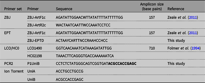
The standard COI barcoding region was amplified for each invertebrate head using up to three primer sets (ZBJ, LCO/HCO, and EPT; Table 1). Specimens were first amplified using primer set ZBJ (Zeale et al. Reference Zeale, Butlin, Barker, Lees and Jones2011) to produce a 157-base-pair amplicon. Samples were amplified in 10-µL reaction volumes using the Qiagen Multiplex polymerase chain reaction kit (catalogue number 206143; Qiagen). Each 10-µL polymerase chain reaction contained 5-µL Multiplex MasterMix (catalogue number 206143: Qiagen Multiplex polymerase chain reaction kit), 0.2-µL forward primer (10 µM), 0.2-µL reverse primer (10 µM), 1.6 µL of nuclease-free water, and 3 µL of extracted DNA. Samples were amplified at 95 ºC for 15 minutes, 39 cycles of 94 ºC for 30 seconds, 52 ºC for 60 seconds, and 72 ºC for 90 seconds, followed by a final extension at 72 ºC for 10 minutes.
Primers used to amplify DNA extracted from individual invertebrate samples and for next-generation sequencing of stomach homogenates on an ion torrent platform. UniA and UniB sequences were included within Zeale et al. (Reference Zeale, Butlin, Barker, Lees and Jones2011) and EPT primers.

If an amplification failed, primer set LCO/HCO was used to amplify the full-length COI barcoding region (Folmer et al. Reference Folmer, Black, Hoeh, Lutz and Vrijenhoek1994). Each 35-µL polymerase chain reaction contained 17.8-µL Multiplex MasterMix, 0.5-µL forward primer (10 µM), 0.5-µL reverse primer (10 µM), and 16.2 µL combined of nuclease-free water, and 20-ng extracted DNA – DNA volume varied by sample based on concentration. The thermocycling parameters were 95 ºC for 15 minutes, 35 cycles of 94 ºC for 60 seconds, 55 ºC for 60 seconds, and 72 ºC for 90 seconds, followed by a final extension at 72 ºC for seven minutes.
If an amplification failed with the first two sets of primers, samples were amplified using primer set EPT, which included the same forward primer as ZBJ (Zeale et al. Reference Zeale, Butlin, Barker, Lees and Jones2011) but with the reverse primer modified to target the most common aquatic Arthropoda in this study (Ephemeroptera, Plecoptera, Trichoptera, and Diptera). These samples were amplified as described for the LCO1490/HC02198 primers but with the same thermal cycling conditions as used for ZBJ. In all cases, polymerase chain reaction products were visualised on 2% TBE agarose gels stained with ethidium bromide to verify the presence of a band at the expected size. Negative extraction and polymerase chain reaction controls were included for each primer set and did not reveal any contamination. Samples that produced amplicons of the desired size were purified using Agencourt AMPure XP purification beads (catalogue number A63881; Beckman and Coulter, Mississauga, Ontario, Canada), and the concentration of the purified polymerase chain reaction product was quantified using a QUBIT 2.0 Fluorometer (catalogue number Q32854: dsDNA High Sensitivity (HS) Assay; Life Technologies, Burlington, Ontario, Canada).
All polymerase chain reaction products were sequenced in the forward direction on an ABI 3130xl genetic analyser (Burlington, Ontario, Canada). Sequences were visualised on CLC Main Workbench 7.6 (Qiagen Bioinformatics, Redwood City, California, United States of America) and manually edited if ambiguous bases were discernible through chromatogram interpretation. To assign taxa, all sequences were compared with publicly available databases, specifically GenBank (Benson et al. Reference Benson, Karsch-Mizrachi, Lipman, Ostell and Wheeler2007) and Biodiversity of Life Database (BOLD) version 3 (Ratnasingham and Hebert Reference Ratnasingham and Hebert2007). Similarities > 95% were considered to be adequate for taxonomic assignment, and taxa were assessed to the lowest corresponding rank. When multiple taxa met this threshold, the rank that was common among them was assigned.
Next-generation sequencing of homogenised stomach samples
Bulk stomach contents removed from the eight rainbow trout and eight prickly sculpin were used for next-generation sequencing analysis and were completed on two separate Ion Torrent sequencing runs. To avoid contamination, all extractions were performed in a room dedicated to low-quality DNA sources as described above. To monitor for contamination, a negative control was included for each set of stomach content DNA extractions.
Stomach samples were centrifuged for one minute at 20 000 × g. Excess ethanol was then decanted, and the stomach contents were transferred into sterile 2-mL centrifuge tubes. Two 5/32-inch steel grinding beads were added to each 2-mL tube and shaken in a Genogrinder 2000 for five minutes at 1500 oscillations/minute. Grinding beads were removed with sterile forceps, and 200 µL of homogenised contents and ethanol were transferred into sterile 1.5-mL centrifuge tubes. Tubes were left open overnight at room temperature in a fume hood for residual ethanol to evaporate. Stomach content samples were extracted using the Qiagen DNeasy Blood and Tissue Kit (spin-column protocol), with the modification of using 2 × 75 µL AE buffer for the final elution step. Deoxyribonucleic acid (DNA) concentration of each bulk sample was quantified using a QUBIT 2.0 Fluorometer (dsDNA HS Assay), and samples were stored at −20 ºC until polymerase chain reaction amplification.
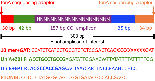
Stomach homogenate samples were prepared for unidirectional sequencing on a PGM Ion Torrent sequencer (Burlington, Ontario) using a two-step polymerase chain reaction amplification method that incorporated fusion primers. In the first polymerase chain reaction step (PCR1), samples were amplified using the EPT primer set, with the primers tailed by the sequences UniA (forward primer) and UniB (reverse primer) (Table 1). The second polymerase chain reaction step (PCR2) incorporated the IonA adaptor (required for the Ion Torrent sequencing reaction), a unique 10-base-pair sequence tag to distinguish each individual sample, and the P1 adaptor required for attaching the prepared amplicons to the Ion Spheres (Fig. 1).
Two-tailed amplicon fusion primer design. First polymerase chain reaction amplifies the 157-base-pair (bp) target sequences of the cytochrome C oxidase subunit I (COI) gene plus primer (ZBJ F and EPT R) and adaptor (UniA and UniB) sequences. Second polymerase chain reaction incorporates the additional IonA and P1 sequencing adaptors and the unique 10-mer sample identification sequence.

For PCR1, three replicates of each homogenised sample were amplified in 35-µL reaction volumes using a Qiagen Multiplex polymerase chain reaction kit (catalogue number 206143). For the first sequencing run, the polymerase chain reactions contained 17.8-µL Multiplex MasterMix, 0.7-µL UniA-tailed ZBJ forward primer (10 µM), 0.7-µL UniB-tailed EPT reverse primer (10 µM), and 15.8-µL combined nuclease-free water and DNA extraction to include 20 ng of DNA. The polymerase chain reactions were modified for the second sequencing run by reducing each primer to 0.5 µL and increasing the water and DNA accordingly. For both sequencing runs, negative extractions and negative polymerase chain reaction controls were included. Samples were amplified at 95 ºC for 15 minutes, 30 cycles of 94 ºC for 30 seconds, 46 ºC for 60 seconds, and 72 ºC for 60 seconds, followed by a final extension at 72 ºC for 10 minutes. Polymerase chain reaction products were visualised on 2% TBE agarose gels stained with ethidium bromide to verify the presence of a single 235-base-pair band (amplicon + primers). First polymerase chain reaction step products were purified using Agencourt AMPure XP purification beads (catalogue number A63881; Beckman and Coulter), and the resulting DNA concentrations were quantified using a QUBIT 2.0 Fluorometer (dsDNA HS Assay).
The second polymerase chain reaction amplification (PCR2) was amplified in 22.5-µL reaction volumes that contained 3.6-µL reaction buffer, 1.5-µL MgCl2 (50 mM), and 0.15-µL Platinum Taq polymerase (5 U/µL) (catalogue number 1096634: all from Invitrogen, Burlington, Ontario, Canada), 0.75-µL dNTPs mix (10 mM) (catalogue number N0446s; New England Biolabs, Ipswich, Massachusetts, United States of America), 0.75-µL IonA-UniA primer (10 µM) (IDT Technologies, Coralville, IA, USA), and 0.75-µL P1-UniB primer (10 µM) (IDT Technologies). The amount of purified PCR1 product added to the reaction varied depending on concentration for a total mass of 30–50 ng of purified PCR1 product per reaction in the first Ion Torrent run and 20–30 ng in the second Ion Torrent run with the volume of nuclease-free water adjusted to a combined volume of 15 µL per run. Second polymerase chain reaction step reactions were amplified at 94 ºC for two minutes, five cycles of 94 ºC for 30 seconds, 60 ºC for 30 seconds, and 72 ºC for 60 seconds, followed by a final extension at 72 ºC for five minutes. Subsets of samples were visualised using the Experion DNA 1 K analysis kit (catalogue number 7007107; Bio-Rad, Mississauga, Ontario, Canada) to verify that the barcodes attached correctly to the PCR1 amplicons. The triplicates of each sample were then pooled (approximately 60 µL), purified with Agencourt AMPure XP purification beads, and quantified using QUBIT 2.0 Fluorometer (dsDNA HS Assay).
Samples were normalised by pooling equimolar ratios of each, including approximately 5 µL of each negative control, which had DNA concentrations that were undetectable by the QUBIT 2.0 Fluorometer. Two 40-µL aliquots of the final normalised COI amplicon library (all samples and negatives controls) were then run on 1.5% TAE agarose gels stained with ethidium bromide at approximately 200 V for 1.5 hours for Ion Torrent run 1 and 100 V for 10 minutes then 150 V for one hour and 50 minutes for Ion Torrent run 2. Run time was increased while using a low voltage at this step to allow for sufficient separation of the 295-base-pair bands (amplicons plus all required adaptor sequences) from those containing amplicons with only one adaptor sequence attached (255 and 275 base pairs). The 295-base-pair fragment was extracted from the gel by visualising the bands on a ultraviolet-light box using a clean, sterile scalpel, and purified using Qiagen MinElute gel extraction kits (catalogue number 28606). The quality and concentration of the COI amplicon libraries were analysed using the Experion DNA 1 K analysis kit and subsequently pooled and submitted to the Great Lakes Institute for Environmental Research Laboratory at the University of Windsor (Windsor, Ontario, Canada), where they were sequenced using an Ion Torrent 318 chip.
Next-generation sequencing data analysis
Two Ion Torrent runs produced 1 116 665 raw reads from the 48 fish stomach homogenate samples (16 samples × three replicates) and 21 negative controls. Sequence cleaning and clustering into operational taxonomic units were performed using USEARCH version 8.1 (Edgar Reference Edgar2010). Primers were removed and barcodes relabelled from reads of each sequencing run fastq file, and then the two were concatenated for subsequent analysis. Sequences were truncated to 157 base pairs to align with the target region of COI and filtered to an expected error threshold of 0.4, which retained 318 521 reads. The expected error value is the sum of each base-pair quality score of a read, indicating a probability that a nucleotide was incorrectly assigned within that read. The reads were dereplicated and chimeras discarded from the sequence data set using the UPARSE algorithm (Edgar Reference Edgar2013). Using the cluster_otus command of UPARSE, each quality filtered read was compared to representative sequences for each operational taxonomic unit and binned using a 97% identity threshold. Combined with the embedded sample name, all reads contained sufficient information for the creation of an operational taxonomic unit table containing 270 operational taxonomic units and 314 363 sequences – 309 279 from the 48 fish samples and 5084 from the 21 negative controls.
To reduce uncertainty associated with unequal sequencing depths between each of the Ion Torrent runs, data were rarefied 10 times to the read count of the least abundant sample, 2045 sequences, using the GUnifrac (Chen Reference Chen2012) package in R, version 3.2.2 (R Core Team 2013). This eliminated one polymerase chain reaction replicate sample from two fish as the total read count in each was too low and resulted in a total of 93 994 sequences and 236 operational taxonomic units. Using polymerase chain reaction replicates as indicators of reliable operational taxonomic unit detection, operational taxonomic units for a fish were removed if they were present in a single replicate only. Operational taxonomic units present in at least two replicates of an individual fish were retained, and sequence counts were evaluated using the average read of the replicates. By eliminating operational taxonomic units which were present in only a single replicate of a given fish, the total number of operational taxonomic units was reduced to 132 and read count to 32 004.
Taxonomic assignment of operational taxonomic units
A blastn search (default parameters; Altschul et al. Reference Altschul, Madden, Schäffer, Zhang, Zhang, Miller and Lipman1997) was conducted for representative sequences of each operational taxonomic unit. Alignment results were imported into MEGAN version 6.5.8 (Huson et al. Reference Huson, Beier, Flade, Górska, El-Hadidi and Mitra2016) where sequences with ≥ 97% match were exported at both the lowest taxonomic level and at the genus level. Taxon verification was conducted by comparing all representative sequences to the BOLD version 3 (Ratnasingham and Hebert Reference Ratnasingham and Hebert2007) with similarities ≥ 97% considered to be successful for species identification. Operational taxonomic units that were assigned identical taxa were combined with their read counts being summed, and those which did not produce a single result (no hit) or were not ≥ 97% (not assigned) were omitted from further analysis. A total of 43 unique genus and species level assignments were made contributing to 194 individual taxonomic detections within the 16 fish. One operational taxonomic unit resulted in a no hit and 23 operational taxonomic units were not assigned.
Statistical analysis
Taxa were condensed at the genus level for statistical analysis, with read counts for operational taxonomic units of identical genera being combined and then transformed to presence/absence data. Nonmetric multidimensional scaling was performed to compare the composition of ingested prey between different fish using PC-Ord version 6.08 (McCune and Mefford Reference McCune and Mefford2011). Nonmetric multidimensional scaling is a rank-based ordination, meaning that although distances between sample units are calculated, the distance matrix is converted to a system that ranks the samples based on their dissimilarity (Minchin Reference Minchin1987) and was conducted according to methods outlined by McCune and Grace (Reference McCune and Grace2002). The ordination was based on a Sorenson’s dissimilarity matrix using PC-Ord in combination with a random starting configuration. Permutational multivariate analysis of variance (PerMANOVA – Sorensen distance measure with 4999 random permutations) was then used to test the difference between fish species based on the presence/absence data set of prey genera.
Results
The mean length (± standard deviation) and weight of the eight rainbow trout used for analysis was 8.0 ± 3.9 cm and 9.1 g (range 1.3–38.5 g) and for the eight prickly sculpin 7.2 ± 2.6 cm and 6.6 g (range 0.9–28.8 g), respectively.
Morphological identification of prey items
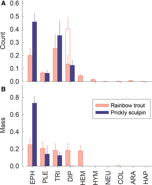
Morphological analyses were performed on 419 invertebrate prey items taken from the gastrointestinal tracts of eight rainbow trout (n = 302) and eight prickly sculpin (n = 117). The average proportional contribution of count data for all fishes combined at the order level suggested rainbow trout fed mainly on Diptera (40%), Trichoptera (25%), Ephemeroptera (20%), and Plecoptera (7%), with the remaining 8% categorised into seven additional invertebrate orders. Approximately, one-third (34%) of the specimens identified in the diet of rainbow trout were terrestrial or adult aquatic insects. Prickly sculpin diet comprised similar orders but mainly consisted of Ephemeroptera (46%) and Trichoptera (35%), with the remaining 19% consisting of Diptera (larvae) (13%) and Plecoptera (6%) (Fig. 2A). Prey mass estimates from rainbow trout revealed that Ephemeroptera (25%), Plecoptera (21%), Trichoptera (18%), Diptera (18%), and Hemiptera (18%) had similar contributions and total > 99% of their diet. Prickly sculpin prey mass estimates suggested their diet consists mainly of Ephemeroptera (73%), with Plecoptera and Trichoptera combining for 26% of the total mass (Fig. 2B).
Average proportional contribution for morphologically identified invertebrate orders sampled from rainbow trout (Oncorhynchus mykiss) (n = 8) and prickly sculpin (Cottus asper) (n = 8) caught in Ormond Creek, British Columbia. A, Count (proportion); B, mass (proportion). Orders are abbreviated as Ephemeroptera (EPH), Plecoptera (PLE), Trichoptera (TRI), Diptera (DIP), Hemiptera (HEM), Hymenoptera (HYM), Neuroptera (NEU), Araneae (ARA), Coleoptera (COL), and Haplotaxida (HAP). Adult (open) and nymph (cross-hatch) stages for the order Diptera were found in the stomachs of rainbow trout (Fig. 2A). No regressions were available for adult Diptera, however, so they are not included in the calculations for mass in Figure 2B. Data are shown as means + standard error.
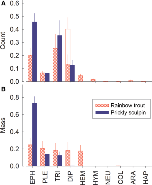
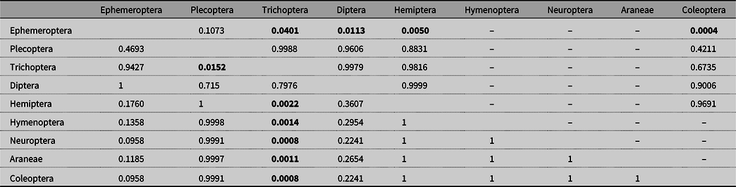
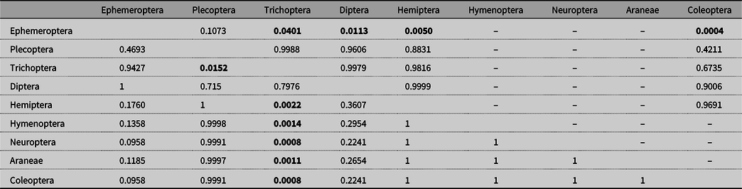
Diet composition varied significantly by invertebrate order for the count data (P < 0.05) and fish species (P < 0.05), while there was no significant interaction between order and fish species (P = 0.215). A significant difference was found between invertebrate orders with Tukey’s post hoc test (Table 2). Analysis of mass data (corrected for individual fish mass) also revealed significant differences in diet composition between orders (P < 0.05), but no effects of fish species (P = 0.118) or interaction (P = 0.350) were found. Post hoc analysis for mass showed significant differences between invertebrate orders (Table 2).
Tukey’s post hoc test for differences between morphologically identified invertebrate orders using all prey items examined from the stomach contents from both rainbow trout (Oncorhynchus mykiss) and prickly sculpin (Cottus asper) (n = 16). Count (below diagonal) and mass (above diagonal) prey data were examined. Bolded values indicate significance at P < 0.05.
Barcoding of individual prey items
From the 419 morphologically identified prey items, 84 full-length barcodes (using LCO/HCO) and 85 shorter barcodes (using ZBJ or EPT) were successfully sequenced and assigned to a taxonomic group with a ≥ 95% match. A further 126 specimens were sequenced but could not be assigned to a taxonomic group. The overall success rate was similar for prey items of rainbow trout and prickly sculpin, 41 and 38%, respectively, with Trichoptera (26%) providing the lowest proportion of successful sequences (Fig. 3A).
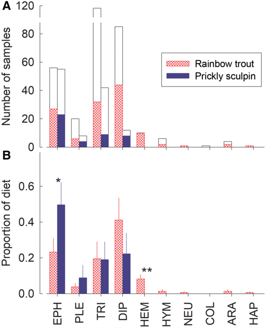
Rainbow trout (Oncorhynchus mykiss) and prickly sculpin (Cottus asper) stomach contents. A, Number of samples extracted for DNA (open bars) and successfully sequenced by barcoding (closed bars) from the stomach contents of rainbow trout (n = 8) and prickly sculpin (n = 8) using the three primers sets; B, proportional comparison of individual prey from rainbow trout and prickly sculpin that produced a barcode sequence that correctly matched their morphological identification (n = 169). Orders are abbreviated as Ephemeroptera (EPH), Plecoptera (PLE), Trichoptera (TRI), Diptera (DIP), Hemiptera (HEM), Hymenoptera (HYM), Neuroptera (NEU), Araneae (ARA), Coleoptera (COL), and Haplotaxida (HAP). Orders that differ significantly by fish species are marked with *(α = 0.10) and **(α = 0.01). Data are shown as means + standard error.
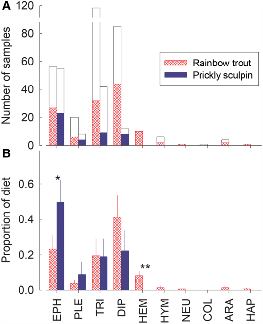
Proportional comparison at the order level showed that Ephemeroptera, Trichoptera, and Diptera were the most abundant prey detected in both fish species, contributing to 84% of the diet for rainbow trout and 91% for prickly sculpin (Fig. 3B). The Diptera (41 ± 12%) component of the diet that included adults and nymphs, however, was significantly greater in rainbow trout, and Ephemeroptera (50 ± 13%) much greater in prickly sculpin.
Next-generation sequencing of homogenised stomach samples
Ion Torrent sequencing of the homogenised stomach contents produced 309 279 high-quality sequences – 49% from rainbow trout and 51% from prickly sculpin – belonging to 270 operational taxonomic units. Following taxonomic assignment and verification of polymerase chain reaction triplicates, operational taxonomic units were condensed into 79 unique taxa, including 59 genera and excluding 56 operational taxonomic units that could not be determined at ≥ 97% identity. This conservative approach led to a final data set including 14 943 reads among 62 unique taxa in the eight rainbow trout and 15 964 reads among 37 unique taxa in the eight prickly sculpin.
The taxa with the highest sequence abundance in rainbow trout diet were Paraleptophlebia heteronea (McDunnough) (Ephemeroptera: Leptophlebiidae) (28%), Ameletus validus McDunnough (Ephemeroptera: Ameletidae) (22%), Lumbricus terrestris Linnaeus (Haplotaxida: Lumbricidae) (11%), Procladius Skuse (Diptera: Chironomidae) (9%), and Skwala compacta (McLachlan) (Plecoptera: Perlodidae) (6%). The most prevalent taxon was Paraleptophlebia heteronea (28%), which was consumed by all eight rainbow trout. Ameletus validus (22%), Lepidostoma Rambur (Trichoptera: Lepidostomatidae) (2%), Cinygmula mimus (Eaton) (Ephemeroptera: Heptageniidae) (< 1%), Micropsectra subletteorum Anderson, Stur, and Ekrem (Diptera: Chironomidae) (< 1%), and Orthocladius van der Wulp (Diptera: Chironomidae) (< 1%), were each consumed by five rainbow trout.
The taxa with the highest sequence abundance in prickly sculpin diet were Paraleptophlebia heteronea (60%), Skwala compacta (14%), Ameletus vernalis McDunnough (Ephemeroptera: Ameletidae) (8%), Ameletus validus (6%), and Drunella grandis (Eaton) (Ephemeroptera: Ephemerellidae) (3%). The most prevalent taxa were Paraleptophlebia heteronea, which were consumed by all eight prickly sculpin; Cinygmula mimus (2%) consumed by seven fish; Limoniidae (Diptera) (1%) consumed by five prickly sculpin; and Ameletus validus, Ameletus vernalis, Paraleptophlebia memorialis (Eaton) (Ephemeroptera: Leptophlebiidae) (1%), and Utacapnia columbiana (Claassen) (Plecoptera: Capniidae) (< 1%), which were each consumed by four prickly sculpin.
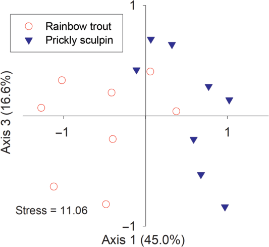
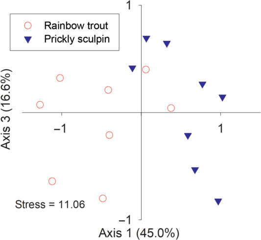
Nonmetric multidimensional scaling analysis of next-generation sequencing prey data indicated a separation in diet composition between rainbow trout and prickly sculpin (Fig. 4). The diet of prickly sculpin was more tightly clustered compared to rainbow trout, implying that there may be more taxonomic variation between the diets of individual rainbow trout. A significant difference in diet (PerMANOVA, F(1,14) = 3.49, P < 0.001) was found between rainbow trout and prickly sculpin based on the analysis of prey genera.
Nonmetric multidimensional scaling ordination of prey genera from rainbow trout (Oncorhynchus mykiss) (n = 8) and prickly sculpin (Cottus asper) (n = 8) sequenced using the Ion Torrent next-generation sequencer.
Comparison of approaches
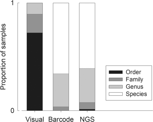
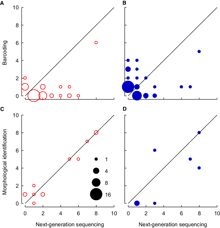
Morphological identification of fish diet typically led to order-level assignments (72%) with family (17%) and genus (10%) being attainable for few of the rainbow trout (Supplementary Table 1) and prickly sculpin (Supplementary Table 2) prey. None of the prey specimens were morphologically identifiable to species. In comparison, identification to genus and species was possible for individually sequenced specimens across nine orders, mainly Ephemeroptera, Plecoptera, Trichoptera, Diptera, and Hemiptera. The greatest number of genera and species were identified from the stomach homogenates that were analysed using next-generation sequencing. From the stomach homogenates, 79 unique taxonomic signatures were identified – 92% were resolved to at least the genus level – compared to 53 unique taxa achieved from barcoding individual specimens (Fig. 5). Both molecular methods identified unique taxa: next-generation sequencing detected 26 genera that were not detected by barcoding, and barcoding detected 17 genera that were not detected by next-generation sequencing (Fig. 6A–B). The genera of rainbow trout prey were more effectively detected using next-generation sequencing compared to prickly sculpin prey, which were, in turn, more effectively detected by barcoding. The use of morphological identification to detect prey at the order level appeared to be similar compared to next-generation sequencing (Fig. 6C–D). This pattern did not change between the fish species, with order-level detection remaining very consistent between the two methods.
Proportional lowest level of taxonomic resolution of samples from stomach contents of rainbow trout (Oncorhynchus mykiss) and prickly sculpin (Cottus asper) determined visually by morphological analysis (n = 419), barcode sequencing of individual prey (n = 169), and next-generation sequencing (NGS) from homogenised stomach contents.

Detection of prey genera using Ion Torrent next-generation sequencing compared to barcode sequencing. A, Rainbow trout (Oncorhynchus mykiss) (n = 8); B, prickly sculpin (Cottus asper) (n = 8). Genera found below the mid line represent greater detection using next-generation sequencing, and genera above the line represent greater detection using barcoding. Detection of orders using Ion Torrent next-generation sequencing compared to morphological identification. C, Rainbow trout; D, prickly sculpin prey. Orders found below the mid line represent greater detection using next-generation sequencing, and orders above the line represent greater detection using morphological identification. Symbol area is proportional to the number of taxa represented by each symbol.

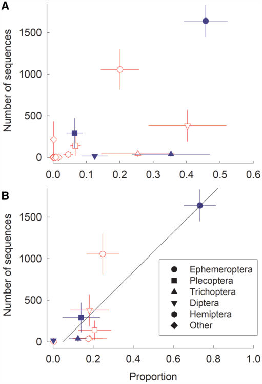
Comparison of the number of sequences produced by next-generation sequencing for each order of aquatic invertebrates to the proportional contribution of the count data of each order revealed little relationship for rainbow trout (F(1,9) = 3.080, P > 0.10) and prickly sculpin (F(1,2) = 1.610, P > 0.30) (Fig. 7A), but there was a significant relationship between sequences and mass data (F(1,8) = 28.39, P < 0.001; Fig. 7B) for data combined as there was no difference in slope between the two species (t = 1.225, P > 0.20).
Number of Ion Torrent next-generation sequencing sequences for each aquatic invertebrate prey order as a function of their proportional contribution from Ormond Creek, British Columbia. A, Count data from rainbow trout (Oncorhynchus mykiss – red open symbols) and prickly sculpin (Cottus asper – blue closed symbols); B, mass data from rainbow trout (red open symbols) and prickly sculpin (blue closed symbols). Data are plotted as means ± standard error.

Discussion
We have shown how molecular tools can be used to assess diversity of semi-digested contents acquired from fish digestive tracts. Tools that allow rapid assessment of aquatic ecosystem biota, particularly related to food chains, represent an important development for the assessment of biodiversity. Molecular methods combined with morphological approaches show tremendous potential for assessing changes associated with anthropogenic activity or natural factors along small streams.
Our fish diet analyses were conducted using three methods, and our study shows the strengths, limitations, and inferences that can be made with each approach. Taxonomic breadth and resolution were best achieved with next-generation sequencing. Barcoding also provided great taxonomic detail on prey items, but poor sequencing success reduced its use in diet analysis. Quantitative data on prey abundance were only available when morphologically identifying prey; however, this method lacks breadth of taxonomic detection and resolution.
Morphological analysis
Morphological analysis allowed the detection of supplemental information on prey items, which can be crucial for understanding diet and predation, such as developmental stage, size, digestion rate, and abundance estimates. Visual identification of invertebrate prey, however, requires a considerable amount of time and expertise to accurately classify even intact specimens to the species level (Lenat and Resh Reference Lenat and Resh2001). The level of digestion and fragmentation of prey obtained from fish digestive tracts restricted identification to order with family and genus being only unreliably attained and resolution to species never achieved. As a result, comparison of diet between rainbow trout and prickly sculpin could only be conducted at the level of order following morphological identification.
While metrics to assess the ecological role of invertebrates in aquatic systems often rely on identification to order, this limitation is often because of the difficulty in rapidly achieving better taxonomic resolution with morphological identification, as was the case in this study. However, better taxonomic resolution may also provide more accurate assessments, for instance, in observing the differences in functional feeding groups (Cummins et al. Reference Cummins, Merritt and Andrade2005), the biomonitoring of streams through invertebrate pollution tolerance levels (Hilsenhoff Reference Hilsenhoff1982; Kerans and Karr Reference Kerans and Karr1994; Diaz et al. Reference Diaz, Solan and Valente2004), and understanding resource partitioning by aquatic invertebrates (Cummins and Klug Reference Cummins and Klug1979; Townsend and Hildrew Reference Townsend and Hildrew1979).
Morphological analysis revealed that in addition to immature aquatic invertebrate prey, rainbow trout diet consisted of a considerable proportion of terrestrial arthropods and adult aquatic insects, indicating predation at or near the water surface by rainbow trout. This is consistent with previous research, which shows juvenile rainbow trout exploit prey throughout the water column, including surface feeding (McPhail Reference McPhail2007). Prickly sculpin are a benthic species whose diet relies on benthic organisms with no substantial terrestrial or adult aquatic invertebrate inputs (McPhail Reference McPhail2007). Morphological analysis of prickly sculpin prey was consistent with an exclusively aquatic diet.
Barcode sequencing
Species-level classifications for invertebrate fragments from the rainbow trout and prickly sculpin stomachs were possible following amplification and sequencing and consistently increased taxonomic resolution over morphological identifications. The detailed description of fish diet obtained using this approach would provide a better understanding of fish predation as invertebrate ecological roles do vary within families or genera (Lenat and Resh Reference Lenat and Resh2001). Inference, however, was limited as less than 50% of the specimens returned usable sequence data. This may be due to the process of digestion and because Sanger sequencing typically requires higher concentrations to properly sequence the target amplicon (Tipu and Shabbir Reference Tipu and Shabbir2015). In addition, although universal primers significantly reduce the cost and time required to perform sequence analysis, primer sets may contain unintended biases against certain taxa resulting in lower binding and amplification success (Sharma and Kobayashi Reference Sharma and Kobayashi2014; Pawluczyk et al. Reference Pawluczyk, Weiss, Links, Egana Aranguren, Wilkinson and Egea-Cortines2015). A combination of these limitations may have contributed to the failure to sequence approximately 60% of the individual specimens. Likely due to these limitations, individual sequencing of invertebrate fragments was also inconsistent across orders – most notably in the Trichoptera where only 26% of sequencing reactions were successful.
Next-generation sequencing
Next-generation sequencing can be used to analyse highly digested arthropods or soft-bodied organisms, which rapidly digest beyond recognition (Symondson Reference Symondson2002; Carreon-Martinez et al. Reference Carreon-Martinez, Johnson, Ludsin and Heath2011). This allows for the identification of a greater diversity of taxa within diet, as was observed in this study where we detected 26 genera that were not detected by morphology or barcoding. Most of the taxa identified using this method were classified with better resolution compared to morphological analysis, which was usually restricted to order, and as such next-generation sequencing of gut contents provided sufficient detail to determine differences between fish diet (Fig. 5), which can also provide ecologically relevant information pertaining to prey items.
Prey analyses rely on quantitative data such as taxonomic abundance or mass to determine prey selection or resource partitioning (Bardach Reference Bardach1962; Hyslop Reference Hyslop1980). Our data indicated that there was no relationship between the number of sequences obtained during next-generation sequencing and abundance, but there was a significant relationship with mass of taxa. Next-generation sequencing methods have not yet been developed to accurately reflect abundance in molecular diet analysis and with other eDNA techniques (Deagle et al. Reference Deagle, Thomas, Shaffer, Trites and Jarman2013; Thomas et al. Reference Thomas, Jarman, Haman, Trites and Deagle2014; Derocles et al. Reference Derocles, Bohan, Dumbrell, Kitson, Massol and Pauvert2018). While this restriction means that these data cannot be applied to prey selection indices, other statistical methods can provide relevant ecological inferences. Our ordination analysis allowed us to determine that the diets of rainbow trout and prickly sculpin were different, and permutational analysis of variance determined this difference to be statistically significant.
Morphological identification appears to be equally effective as molecular methods for the detection of invertebrate orders in fish but much less effective at assigning lower taxonomic levels. While this means that quantitative data can be obtained from morphological analyses, it is important to consider the lack of apparent functional diversity within aquatic invertebrates when viewed from the order level. When coupled with sequencing of individual organisms, morphological identification can provide quantitative and natural history data that would be impossible with next-generation sequencing. A morphology-plus-barcoding protocol thus provides advantages but is hindered by the ability to successfully sequence tiny specimens in a digestive context. Next-generation sequencing provided the most exhaustive description of taxa in fish diets and likely approximates the complete diversity of organisms that contribute to their diets – although biases against certain taxa will also occur with next-generation sequencing analysis. Morphological analysis, barcoding, and next-generation sequencing approaches to examine stomach contents provided complementary information on rainbow trout and prickly sculpin diets and should each be used alone or in different combinations depending on the analytical context. While the best possible resolution might come from very comprehensive barcoding of gut contents, the expense, the time required, and the loss of sequence data inherent to that technique likely preclude such a use in most situations.
Acknowledgements
We thank Angela Grob, Kacie Young, Charles Bradshaw, Rick Elsner, and Daemon Cline for assistance with field sampling and sample preparation; Caitlin Pitt for sequence analysis at the University of Northern British Columbia; and Dr. Aynsley Thielman and Dr. Nicole Sukdeo for assistance and suggestions for statistics and laboratory approaches. We appreciate the input and assistance with next-generation sequencing from Russ Hepburn, Great Lakes Institute for Environment Research and Department of Biology, University of Windsor. We are grateful to Dr. Michael Gillingham and Dr. Jeanne Robert for initiation and management of the Biodiversity Monitoring and Assessment Programme. We thank Dr. Cory Sheffield and two anonymous reviewers for their comments and suggestions that improved the manuscript. This project was funded by the Pacific Trail Pipeline Limited Partnership and Natural Sciences and Engineering Research Council of Canada Discovery grants to J.M.S. and D.P.W.H.
Supplementary material
To view supplementary material for this article, please visit https://doi.org/10.4039/tce.2020.25.