1 Introduction
An important task for minimizing the devastation of tsunamis is to establish a comprehensive and reliable early-warning system. Currently this task is largely based on the detection of the front of the surface gravity waves by measuring either the movement of dart buoys or the bottom pressure at many stations in the ocean. Guided by the key parameters of the fault estimated from seismic observations, these records are used to supply the initial and boundary conditions for computational models of hydrodynamics. So far, these operational models are based on the assumptions of an incompressible fluid, where only gravity is accounted for as a restoring force.
In an ocean of depth
 $h=4000~\text{m}$
, the phase speed of a tsunami front
 $\sqrt{gh}$
is approximately
 $200~\text{m}~\text{s}^{-1}$
, whereas the speed of sound in water is far greater, at
 $c=1500~\text{m}~\text{s}^{-1}$
. Hence, ideas for earlier detection of tsunamis from the acoustic forerunner have attracted some attention in the recent past. A number of authors have studied unidirectional acoustic–gravity waves from an infinitely long fault by including water compressibility and gravity (Miyoshi Reference Miyoshi1954; Sells Reference Sells1965; Kajiura Reference Kajiura1970; Yamamoto Reference Yamamoto1982; Nosov Reference Nosov1999; Nosov & Kolesov Reference Nosov and Kolesov2007; Chierici et al. Reference Chierici, Pignagnoli and Embriaco2010; Stiassnie Reference Stiassnie2010; Kadri & Stiassnie Reference Kadri and Stiassnie2013; Kadri & Akylas Reference Kadri and Akylas2016). However, all of these cited studies show that sound and gravity waves are virtually decoupled after a long distance of propagation, due to the disparate speeds. In particular, Stiassnie derived a simple asymptotic approximation of the leading waves and showed explicitly that, if the distance between the source and target is great, sound signals can clearly outrun the gravity waves at the front. For two-dimensional faults of finite size in a sea of constant depth, Hendin & Stiassnie (Reference Hendin and Stiassnie2013) reported a three-dimensional theory of acoustic–gravity waves based on the classical method of the Green’s function. Contributions from the acoustic and gravity waves were shown to be expressed by two separate integrals. For an elongated rectangular fault, some computational efforts were required to evaluate the integral over the area of source distribution. (For a rectangular fault of
 $40~\text{km}$
by
 $800~\text{km}$
, 32 000 discrete elements of
 $1~\text{km}^{2}$
size were needed to compute the far field
 $1000~\text{km}$
away from the fault.) They further introduced an ingenious inverse theory to predict major features of the fault based on data from two remote hydrophones. For two-dimensional bathymetry and fault area, the mild-slope equation originated for gravity waves has recently been extended to acoustic–gravity waves by Sammarco et al. (Reference Sammarco, Cecioni, Bellotti and Abdolali2013) and Abdolali, Kirby & Bellotti (Reference Abdolali, Kirby and Bellotti2015). To cover an area of many wavelengths in each horizontal direction, a numerical solution requires a huge number of discrete elements much smaller than a wavelength. Hence, this scheme demands non-trivial computational effort for trans-ocean sound signals from two-dimensional fault and bathymetry, as is well known in the case of pure gravity waves. So far these two-dimensional mild-slope equations have been numerically demonstrated only for a one-dimensional fault and bathymetry, using 2500 discrete elements (Abdolali et al.
Reference Abdolali, Kirby and Bellotti2015).
In this work our objective is to seek alternative theories for cases where the submarine epicentre is very far from the target region. Since the acoustic precursor can arrive at a distant target considerably earlier than the gravity waves, it is mathematically simpler to treat the acoustic and gravity waves separately. Indeed, we shall show that by focusing on the acoustic effects alone, the front-running part in Stiassnie’s (Reference Stiassnie2010) theory for a unidirectional tsunami can be quickly recovered. With this simplification, we find an explicit analytical solution for two-dimensional sound radiated from a slender fault of finite size.
Since the fault of a submarine earthquake is often slender in shape (see table 1), the forward (or backward) radiation must differ from that in the lateral directions. For these cases, approximate three-dimensional analyses are desirable to expedite the theoretical understanding. In particular, two-dimensional variations in the open ocean are affected by several much greater length scales, which are sharply different in the forward and lateral directions. Using this contrast, we start from the acoustic equations without gravity and show first that, within a distance not too far from the fault, sound is essentially unidirectional, as predicted by the front-running part of the acoustic–gravity wave theory of Stiassnie (Reference Stiassnie2010). However, over much longer distances, the finite size of the slender fault leads to variations of the wave envelope being evident in both forward and lateral directions. Analytical results for a sea of constant depth are employed to calculate the sound signal of the tsunami front from a medium-sized fault to an area thousands of kilometres away. The inverse theory of Hendin & Stiassnie (Reference Hendin and Stiassnie2013) is then applied to predict explicitly the main fault features from recordings at two distant hydrophones. For slowly varying sea depth, the multiple-scale approximation can be extended to reduce the numerical effort. The approximate envelope equation for non-uniform but slowly varying sea depth is outlined in appendix B.
Underwater sound propagation is of course a topic important to the tracking of ships and marine animals, and in the survey of seabed properties and topography. In nature, ocean acoustics should involve other complex factors, such as coastline reflection and scattering by bathymetric variations (Kadri Reference Kadri2015) and by surface gravity waves (Brekhovskikh & Lysanov Reference Brekhovskikh and Lysanov1991), as well as dissipation by fluid viscosity, friction on the rough seabed, and through marine sediments (Stoll Reference Stoll1977), etc. In principle, elastic waves of Rayleigh and Scholte class can exist along the sea floor. It has been shown by Eyov et al. (Reference Eyov, Klar, Kadri and Stiassnie2013) that, for monochromatic waves in a sea of constant depth
 $h$
over an elastic half-space, the vertical ground displacement is only
 $O(10^{-6})$
times that of the free surface if the frequency is
 $f=0.167~\text{Hz}$
, corresponding roughly to the radian frequency of the most energetic acoustic mode
 $\unicode[STIX]{x1D714}_{1}=\unicode[STIX]{x03C0}c/2h$
for
 $h=4~\text{km}$
. These effects are not considered here. For slender faults, modifications of the present approach to incorporate these additional effects are possible to reduce future modelling efforts.
Key data of some recent tsunamis. The sea depth is approximately
 $4~\text{km}$
in all cases above. From the lecture by Philip L.-F. Liu, in Tsunami and storm surges, Valparaiso, Chile, 2–13 January 2013.

2 Governing equations and approximations
We assume the sea water to be slightly compressible. For the dominant acoustic mode in a sea of depth
 $h$
,
 $\unicode[STIX]{x1D714}_{1}=\unicode[STIX]{x03C0}c/2h$
, the viscous damping rate is roughly
 $O(10^{-8})~\text{dB}~\text{km}^{-1}$
if
 $h=4~\text{km}$
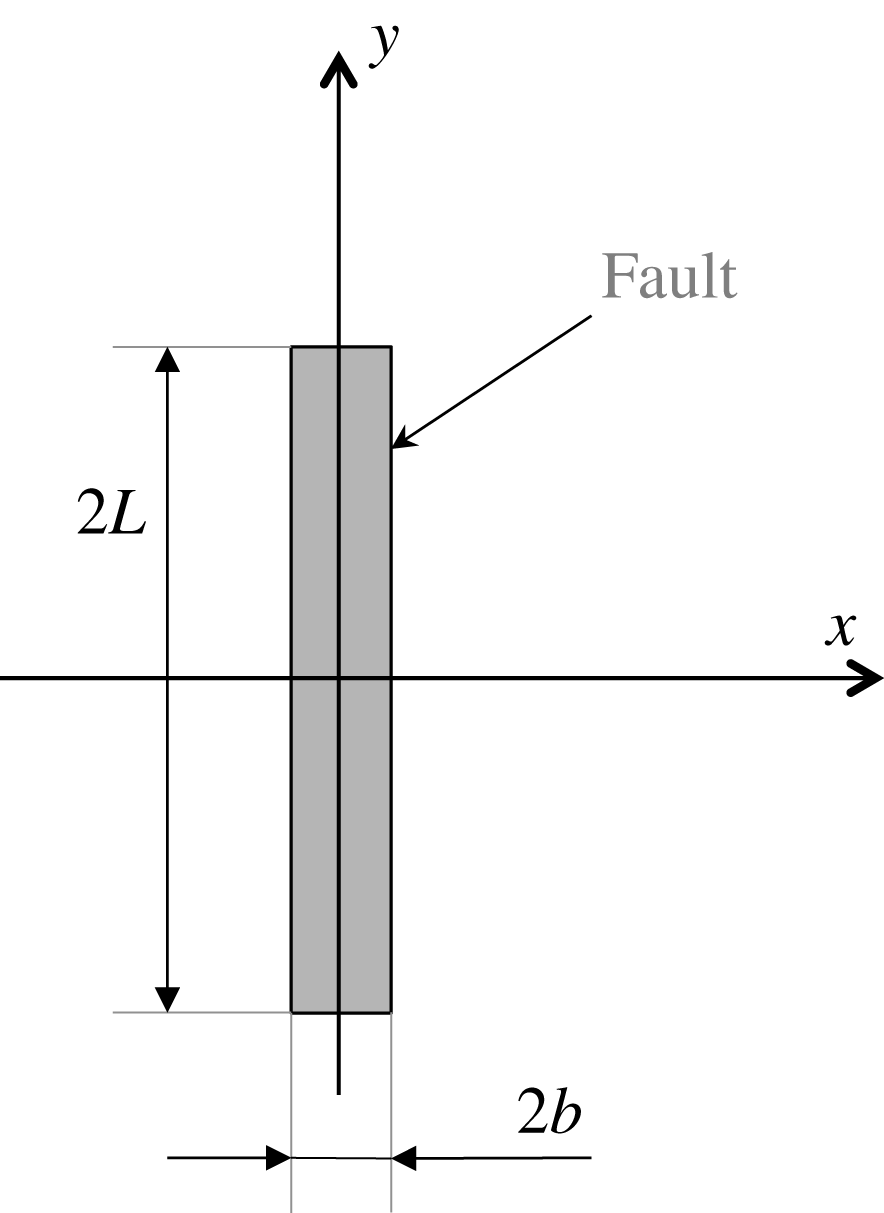
(by extrapolation from Brekhovskikh & Lysanov (Reference Brekhovskikh and Lysanov1991) and Denny (Reference Denny1993)). Hence viscosity is negligible and the flow is irrotational, as is commonly assumed in ocean acoustics. With reference to the coordinate system defined in figure 1, the velocity potential
 $\unicode[STIX]{x1D719}$
of the sound wave is governed by the standard wave equation
 $$\begin{eqnarray}\frac{\unicode[STIX]{x2202}^{2}\unicode[STIX]{x1D719}}{\unicode[STIX]{x2202}x^{2}}+\frac{\unicode[STIX]{x2202}^{2}\unicode[STIX]{x1D719}}{\unicode[STIX]{x2202}y^{2}}+\frac{\unicode[STIX]{x2202}^{2}\unicode[STIX]{x1D719}}{\unicode[STIX]{x2202}z^{2}}=\frac{1}{c^{2}}\frac{\unicode[STIX]{x2202}^{2}\unicode[STIX]{x1D719}}{\unicode[STIX]{x2202}t^{2}}.\end{eqnarray}$$
On the free surface
 $z=h$
the atmospheric pressure is assumed to be uniform and taken to be zero:
 $$\begin{eqnarray}\unicode[STIX]{x1D719}=0,\quad z=h.\end{eqnarray}$$
On the horizontal seabed
 $z=0$
, the ground motion due to seismic rupture is confined in a rectangular strip of width
 $2b$
and length
 $2L$
:
 $$\begin{eqnarray}\frac{\unicode[STIX]{x2202}\unicode[STIX]{x1D719}}{\unicode[STIX]{x2202}z}=W(x,y,t),\quad |x|<b,|y|<L,z=0.\end{eqnarray}$$
Coordinates of a slender fault in the horizontal plane.

As a numerical guide, we shall consider a medium-to-large earthquake where the typical sea depth
 $h=4~\text{km}$
, and a slender fault of width
 $b=O(10)~\text{km}$
and length
 $L=O(100)~\text{km}$
. Hence we assume
 $$\begin{eqnarray}\frac{b}{L}=\unicode[STIX]{x1D716}\ll 1.\end{eqnarray}$$
Owing to reflections from the seabed and the sea surface, many acoustic modes are generated. The frequency of the fundamental mode can be estimated as
 $\unicode[STIX]{x1D714}_{1}=\unicode[STIX]{x03C0}c/2h$
(see (3.9)) where
 $c=1500~\text{m}~\text{s}^{-1}$
is the sound speed in water. Using
 $h=4~\text{km}$
as an estimate, we find the corresponding sound wave period to be
 $10.6~\text{s}$
and wavelength to be
 $16~\text{km}$
. To predict trans-ocean propagation of
 $O(1000)~\text{km}$
or more, we introduce multiple-scale coordinates as
 $$\begin{eqnarray}x,~z;~X=\unicode[STIX]{x1D716}^{2}x,~Y=\unicode[STIX]{x1D716}y,\end{eqnarray}$$
and rewrite the wave equation as
 $$\begin{eqnarray}\left(\frac{\unicode[STIX]{x2202}^{2}}{\unicode[STIX]{x2202}x^{2}}+2\unicode[STIX]{x1D716}^{2}\frac{\unicode[STIX]{x2202}^{2}}{\unicode[STIX]{x2202}x\unicode[STIX]{x2202}X}+\unicode[STIX]{x1D716}^{2}\frac{\unicode[STIX]{x2202}^{2}}{\unicode[STIX]{x2202}Y^{2}}+\frac{\unicode[STIX]{x2202}^{2}}{\unicode[STIX]{x2202}z^{2}}\right)\unicode[STIX]{x1D719}=\frac{1}{c^{2}}\frac{\unicode[STIX]{x2202}^{2}\unicode[STIX]{x1D719}}{\unicode[STIX]{x2202}t^{2}},\quad 0<z<h.\end{eqnarray}$$
Let
 $$\begin{eqnarray}\unicode[STIX]{x1D719}=\unicode[STIX]{x1D719}_{0}(x,X,Y,z)+\unicode[STIX]{x1D716}^{2}\unicode[STIX]{x1D719}_{2}(x,X,Y,z)+\cdots \,.\end{eqnarray}$$
The perturbation equations at
 $O(1)$
describe the two-dimensional physics only,
 $$\begin{eqnarray}\frac{\unicode[STIX]{x2202}^{2}\unicode[STIX]{x1D719}_{0}}{\unicode[STIX]{x2202}z^{2}}+\frac{\unicode[STIX]{x2202}^{2}\unicode[STIX]{x1D719}_{0}}{\unicode[STIX]{x2202}x^{2}}-\frac{1}{c^{2}}\frac{\unicode[STIX]{x2202}^{2}\unicode[STIX]{x1D719}_{0}}{\unicode[STIX]{x2202}t^{2}}=0,\quad 0<z<h,\end{eqnarray}$$
subjected to the boundary conditions
 $$\begin{eqnarray}\unicode[STIX]{x1D719}_{0}=0,\quad z=h\end{eqnarray}$$
and
 $$\begin{eqnarray}\frac{\unicode[STIX]{x2202}\unicode[STIX]{x1D719}_{0}}{\unicode[STIX]{x2202}z}=\left\{\begin{array}{@{}ll@{}}W(x,Y,t), & |x|<b,~|Y|<\ell =\unicode[STIX]{x1D716}L,\\ 0, & \text{elsewhere,}\end{array}\right.\quad z=0,\end{eqnarray}$$
where
 $X$
and
 $Y$
are only parameters.
At
 $O(\unicode[STIX]{x1D716}^{2})$
we have
 $$\begin{eqnarray}\frac{\unicode[STIX]{x2202}^{2}\unicode[STIX]{x1D719}_{2}}{\unicode[STIX]{x2202}z^{2}}+\frac{\unicode[STIX]{x2202}^{2}\unicode[STIX]{x1D719}_{2}}{\unicode[STIX]{x2202}x^{2}}-\frac{1}{c^{2}}\frac{\unicode[STIX]{x2202}^{2}\unicode[STIX]{x1D719}_{2}}{\unicode[STIX]{x2202}t^{2}}=-\!\left\{\frac{\unicode[STIX]{x2202}^{2}\unicode[STIX]{x1D719}_{0}}{\unicode[STIX]{x2202}Y^{2}}+2\frac{\unicode[STIX]{x2202}^{2}\unicode[STIX]{x1D719}_{0}}{\unicode[STIX]{x2202}x\unicode[STIX]{x2202}X}\right\},\quad 0<z<h,\end{eqnarray}$$
with
 $$\begin{eqnarray}\unicode[STIX]{x1D719}_{2}=0,\quad z=h\end{eqnarray}$$
and
 $$\begin{eqnarray}\frac{\unicode[STIX]{x2202}\unicode[STIX]{x1D719}_{2}}{\unicode[STIX]{x2202}z}=0,\quad z=0.\end{eqnarray}$$
3 Leading-order potential
 $\unicode[STIX]{x1D719}_{0}$

For analytical simplicity we assume the ground uplift to be of top-hat form:
 $$\begin{eqnarray}\frac{\unicode[STIX]{x2202}\unicode[STIX]{x1D719}_{0}}{\unicode[STIX]{x2202}z}=w(x,Y)\unicode[STIX]{x1D70F}(t),\quad z=0,\end{eqnarray}$$
where
 $$\begin{eqnarray}w(x,Y)=\left\{\begin{array}{@{}ll@{}}W_{0}=\text{const.}, & |x|<b,~|Y|<\ell ,\\ 0, & \text{elsewhere,}\end{array}\right.\quad \unicode[STIX]{x1D70F}(t)=\left\{\begin{array}{@{}ll@{}}1, & -T<t<T,\\ 0, & |t|>T,\end{array}\right.\end{eqnarray}$$
with
 $\ell =O(\unicode[STIX]{x1D716}L)=O(b/\unicode[STIX]{x1D716})$
. By double Fourier transformation
 $$\begin{eqnarray}\bar{\unicode[STIX]{x1D719}}_{0}=\int _{-\infty }^{\infty }\text{e}^{\text{i}\unicode[STIX]{x1D714}t}\unicode[STIX]{x1D719}_{0}\,\text{d}t,\quad \unicode[STIX]{x1D6F7}=\int _{-\infty }^{\infty }\text{e}^{-\text{i}kx}\bar{\unicode[STIX]{x1D719}}_{0}\,\text{d}x,\end{eqnarray}$$
we readily find
 $$\begin{eqnarray}\unicode[STIX]{x1D6F7}=-W_{0}\frac{G}{\unicode[STIX]{x1D707}}\frac{\sin \unicode[STIX]{x1D707}(h-z)}{\cos \unicode[STIX]{x1D707}h},\end{eqnarray}$$
where
 $$\begin{eqnarray}W_{0}G(k,\unicode[STIX]{x1D714})=\int _{-\infty }^{\infty }\text{e}^{-\text{i}kx}w(x,Y)\,\text{d}x\int _{-\infty }^{\infty }\text{e}^{\text{i}\unicode[STIX]{x1D714}t}\unicode[STIX]{x1D70F}(t)\,\text{d}t=4W_{0}\frac{\sin (kb)\sin (\unicode[STIX]{x1D714}T)}{k\unicode[STIX]{x1D714}}\end{eqnarray}$$
and
 $$\begin{eqnarray}\displaystyle & \displaystyle \unicode[STIX]{x1D707}=\sqrt{\frac{\unicode[STIX]{x1D714}^{2}}{c^{2}}-k^{2}}, & \displaystyle\end{eqnarray}$$
 $$\begin{eqnarray}\displaystyle & \displaystyle \unicode[STIX]{x1D719}_{0}=-\frac{W_{0}(Y)}{2\unicode[STIX]{x03C0}2\unicode[STIX]{x03C0}}\int _{-\infty }^{\infty }\,\text{d}\unicode[STIX]{x1D714}\,\text{e}^{-\text{i}\unicode[STIX]{x1D714}t}\int _{-\infty }^{\infty }\text{d}k\,\text{e}^{\text{i}kx}\frac{G(k,\unicode[STIX]{x1D714})}{\unicode[STIX]{x1D707}}\frac{\sin \unicode[STIX]{x1D707}(h-z)}{\cos \unicode[STIX]{x1D707}h}. & \displaystyle\end{eqnarray}$$
The inversion can be completed by the standard method of residue calculus, as sketched in appendix A, with the result
 $$\begin{eqnarray}\displaystyle \displaystyle \unicode[STIX]{x1D719}_{0} & = & \displaystyle -\frac{W_{0}}{\unicode[STIX]{x03C0}}\,\text{Re}\int _{\unicode[STIX]{x1D714}_{N}}^{\infty }\text{i}\,\text{d}\unicode[STIX]{x1D714}\,\text{e}^{-\text{i}\unicode[STIX]{x1D714}t}\mathop{\sum }_{1}^{N}\frac{G(k_{n},\unicode[STIX]{x1D714})}{k_{n}h}\frac{\sin \unicode[STIX]{x1D707}_{n}(h-z)}{\sin \unicode[STIX]{x1D707}_{n}h}\text{e}^{\text{i}k_{n}|x|}\nonumber\\ \displaystyle & & \displaystyle -\,\frac{W_{0}}{\unicode[STIX]{x03C0}}\int _{0}^{\unicode[STIX]{x1D714}_{N}}\text{d}\unicode[STIX]{x1D714}\cos (\unicode[STIX]{x1D714}t)\mathop{\sum }_{N+1}^{\infty }\frac{G(\unicode[STIX]{x1D706}_{n},\unicode[STIX]{x1D714})}{\unicode[STIX]{x1D706}_{n}h}\frac{\sin \unicode[STIX]{x1D707}_{n}(h-z)}{\sin \unicode[STIX]{x1D707}_{n}h}\text{e}^{-\unicode[STIX]{x1D706}_{n}|x|},\end{eqnarray}$$
where
 $$\begin{eqnarray}\unicode[STIX]{x1D707}_{n}=\left(n-\frac{1}{2}\right)\frac{\unicode[STIX]{x03C0}}{h}\,\equiv \,\frac{\unicode[STIX]{x1D714}_{n}}{c},\quad n=1,2,3,\ldots\end{eqnarray}$$
is a real zero of
 $\cos \unicode[STIX]{x1D707}h=0$
. It follows from (3.6) that
 $$\begin{eqnarray}k_{n}=\frac{\sqrt{\unicode[STIX]{x1D714}^{2}-\unicode[STIX]{x1D714}_{n}^{2}}}{c}\end{eqnarray}$$
is real if
 $\unicode[STIX]{x1D714}^{2}>\unicode[STIX]{x1D714}_{n}^{2}$
. Let
 $\unicode[STIX]{x1D714}_{N}$
be the largest
 $\unicode[STIX]{x1D714}_{n}$
satisfying this inequality; then only
 $k_{1}>k_{2}>\cdots >k_{N}$
are real. If, on the other hand,
 $\unicode[STIX]{x1D714}^{2}<\unicode[STIX]{x1D714}_{N}^{2}$
,
 $k_{n}=\text{i}\unicode[STIX]{x1D706}_{n}$
is imaginary, with
 $$\begin{eqnarray}\unicode[STIX]{x1D706}_{n}=\frac{\sqrt{\unicode[STIX]{x1D714}_{n}^{2}-\unicode[STIX]{x1D714}^{2}}}{c},\quad n=N+1,N+2,\ldots ~\text{and}~\unicode[STIX]{x1D706}_{N+1}<\unicode[STIX]{x1D706}_{N+2}<\cdots \,.\end{eqnarray}$$
The bottom pressure is given by the linearized Bernoulli equation,
 $$\begin{eqnarray}\displaystyle & & \displaystyle \displaystyle p=-\unicode[STIX]{x1D70C}\left.\frac{\unicode[STIX]{x2202}\unicode[STIX]{x1D719}_{0}}{\unicode[STIX]{x2202}t}\right|_{z=0}=-\unicode[STIX]{x1D70C}\frac{W_{0}}{\unicode[STIX]{x03C0}}\,\text{Re}\int _{\unicode[STIX]{x1D714}_{N}}^{\infty }\unicode[STIX]{x1D714}\,\text{d}\unicode[STIX]{x1D714}\,\text{e}^{-\text{i}\unicode[STIX]{x1D714}t}\mathop{\sum }_{1}^{N}\frac{G(k_{n},\unicode[STIX]{x1D714})}{k_{n}h}\,\text{e}^{\text{i}k_{n}|x|}\nonumber\\ \displaystyle & & \displaystyle \displaystyle \qquad +\,\unicode[STIX]{x1D70C}\frac{W_{0}}{\unicode[STIX]{x03C0}}\int _{0}^{\unicode[STIX]{x1D714}_{N}}\unicode[STIX]{x1D714}\,\text{d}\unicode[STIX]{x1D714}\sin (\unicode[STIX]{x1D714}t)\mathop{\sum }_{N+1}^{\infty }\frac{G(\unicode[STIX]{x1D706}_{n},\unicode[STIX]{x1D714})}{\unicode[STIX]{x1D706}_{n}h}\,\text{e}^{-\unicode[STIX]{x1D706}_{n}|x|}.\end{eqnarray}$$
In (3.8) and (3.12), the first series represents the propagating modes, whereas the second corresponds to evanescent modes that decay exponentially with distance and is not important far from the source. Note that (3.8) and (3.12) are exact, but can only describe the physics in the small neighbourhood of
 $O(x,y)\leqslant b$
. For trans-ocean application, an improvement for the study of long-distance evolution must now be found.
4 Improvement for long-range modulation
Let us consider the region
 $x>0$
far away to the right of the fault. Anticipating that the propagating modes have slowly varying envelopes, we introduce unknown envelope factors
 $A_{n}^{\pm }(X,Y)$
and rewrite (3.8) as
 $$\begin{eqnarray}\displaystyle & & \displaystyle \displaystyle \unicode[STIX]{x1D719}_{0}=-\frac{W_{0}}{2\unicode[STIX]{x03C0}}\left\{\int _{\unicode[STIX]{x1D714}_{N}}^{\infty }\text{i}\,\text{d}\unicode[STIX]{x1D714}\,\text{e}^{-\text{i}\unicode[STIX]{x1D714}t}\mathop{\sum }_{1}^{N}A_{n}^{+}\frac{G(k_{n})}{k_{n}h}\frac{\sin \unicode[STIX]{x1D707}_{n}(h-z)}{\sin \unicode[STIX]{x1D707}_{n}h}\text{e}^{\text{i}k_{n}|x|}\right.\nonumber\\ \displaystyle & & \displaystyle \displaystyle \qquad \left.-\int _{-\infty }^{-\unicode[STIX]{x1D714}_{N}}\text{i}\,\text{d}\unicode[STIX]{x1D714}\,\text{e}^{-\text{i}\unicode[STIX]{x1D714}t}\mathop{\sum }_{1}^{N}A_{n}^{-}\frac{G(k_{n})}{k_{n}h}\frac{\sin \unicode[STIX]{x1D707}_{n}(h-z)}{\sin \unicode[STIX]{x1D707}_{n}h}\text{e}^{-\text{i}k_{n}|x|}\right\}\nonumber\\ \displaystyle & & \displaystyle \displaystyle \qquad -\,\frac{W_{0}}{2\unicode[STIX]{x03C0}}\left[\int _{-\unicode[STIX]{x1D714}_{N}}^{0}+\int _{0}^{\unicode[STIX]{x1D714}_{N}}\right]\text{i}\,\text{d}\unicode[STIX]{x1D714}\,\text{e}^{-\text{i}\unicode[STIX]{x1D714}t}\mathop{\sum }_{N+1}^{\infty }\frac{G(\text{i}\unicode[STIX]{x1D706}_{n})}{\text{i}\unicode[STIX]{x1D706}_{n}h}\frac{\sin \unicode[STIX]{x1D707}_{n}(h-z)}{\sin \unicode[STIX]{x1D707}_{n}h}\text{e}^{-\unicode[STIX]{x1D706}_{n}|x|}.\end{eqnarray}$$
The envelope factors of the evanescent modes are trivially
 $A_{n}\,\equiv \,1$
since they vanish in the far field. We shall now search for the equation governing
 $A_{n}^{\pm }(X,Y)$
, which are expected to satisfy the initial conditions:
 $$\begin{eqnarray}A_{n}^{\pm }=\left\{\begin{array}{@{}ll@{}}1, & |Y|<\ell =\unicode[STIX]{x1D716}L,\\ 0, & |Y|>\ell =\unicode[STIX]{x1D716}L,\end{array}\right.\quad X=\unicode[STIX]{x1D716}^{2}x\rightarrow 0.\end{eqnarray}$$
Let us take the time-Fourier transform of (2.11) and separate
 $\bar{\unicode[STIX]{x1D719}}_{2}$
into three different ranges of
 $\unicode[STIX]{x1D714}$
, as follows:
 $$\begin{eqnarray}\bar{\unicode[STIX]{x1D719}}_{2}=\left\{\begin{array}{@{}ll@{}}\bar{\unicode[STIX]{x1D719}}_{2}^{+}, & \unicode[STIX]{x1D714}_{N}<\unicode[STIX]{x1D714}<\infty ,\\ \bar{\unicode[STIX]{x1D719}}_{2}^{e}, & -\unicode[STIX]{x1D714}_{N}<\unicode[STIX]{x1D714}<\unicode[STIX]{x1D714}_{N},\\ \bar{\unicode[STIX]{x1D719}}_{2}^{-}, & -\unicode[STIX]{x1D714}_{N}>\unicode[STIX]{x1D714}>-\infty .\end{array}\right.\end{eqnarray}$$
In the range of
 $\unicode[STIX]{x1D714}_{N}<\unicode[STIX]{x1D714}<\infty$
,
 $$\begin{eqnarray}\frac{\unicode[STIX]{x2202}^{2}\bar{\unicode[STIX]{x1D719}}_{2}^{+}}{\unicode[STIX]{x2202}x^{2}}+\frac{\unicode[STIX]{x2202}^{2}\bar{\unicode[STIX]{x1D719}}_{2}^{+}}{\unicode[STIX]{x2202}z^{2}}+\frac{\unicode[STIX]{x1D714}^{2}}{c^{2}}\bar{\unicode[STIX]{x1D719}}_{2}^{+}=-\text{i}W_{0}\mathop{\sum }_{1}^{N}\left[\frac{\unicode[STIX]{x2202}^{2}A_{n}^{+}}{\unicode[STIX]{x2202}Y^{2}}+2\text{i}k_{n}(\text{sgn}~x)\frac{\unicode[STIX]{x2202}A_{n}^{+}}{\unicode[STIX]{x2202}X}\right]\frac{G(k_{n},\unicode[STIX]{x1D714})}{k_{n}h}\frac{\sin \unicode[STIX]{x1D707}_{n}(h-z)}{\sin \unicode[STIX]{x1D707}_{n}h}\text{e}^{\text{i}k_{n}|x|}.\end{eqnarray}$$
Assuming
 $$\begin{eqnarray}\bar{\unicode[STIX]{x1D719}}_{2}^{+}=\mathop{\sum }_{n=1}^{N}\unicode[STIX]{x1D713}_{n}^{+}(\unicode[STIX]{x1D714},z)\text{e}^{\text{i}k_{n}|x|},\end{eqnarray}$$
then
 $$\begin{eqnarray}\frac{\unicode[STIX]{x2202}^{2}\unicode[STIX]{x1D713}_{n}^{+}}{\unicode[STIX]{x2202}z^{2}}+\unicode[STIX]{x1D707}_{n}^{2}\unicode[STIX]{x1D713}_{n}^{+}=-\text{i}W_{0}\left[\frac{\unicode[STIX]{x2202}^{2}A_{n}^{+}}{\unicode[STIX]{x2202}Y^{2}}+2\text{i}k_{n}(\text{sgn}~x)\frac{\unicode[STIX]{x2202}A_{n}^{+}}{\unicode[STIX]{x2202}X}\right]\frac{G(k_{n},\unicode[STIX]{x1D714})}{k_{n}h}F_{n}(z)\end{eqnarray}$$
subjected to the boundary conditions
 $$\begin{eqnarray}\unicode[STIX]{x1D713}_{n}^{+}=0,\quad z=h\quad \text{and}\quad \frac{\unicode[STIX]{x2202}\unicode[STIX]{x1D713}_{n}^{+}}{\unicode[STIX]{x2202}z}=0,\quad z=0,\end{eqnarray}$$
where
 $$\begin{eqnarray}F_{n}=\frac{\sin \unicode[STIX]{x1D707}_{n}(h-z)}{\sin \unicode[STIX]{x1D707}_{n}h},\end{eqnarray}$$
which is an eigen-solution of the homogeneous boundary value problem
 $$\begin{eqnarray}\displaystyle & \displaystyle \frac{\unicode[STIX]{x2202}^{2}F_{n}}{\unicode[STIX]{x2202}z^{2}}+\unicode[STIX]{x1D707}_{n}^{2}F_{n}=0, & \displaystyle\end{eqnarray}$$
 $$\begin{eqnarray}\displaystyle & \displaystyle F_{n}=0,\quad z=h, & \displaystyle\end{eqnarray}$$
 $$\begin{eqnarray}\displaystyle & \displaystyle \frac{\unicode[STIX]{x2202}F_{n}}{\unicode[STIX]{x2202}z}=0,\quad z=0. & \displaystyle\end{eqnarray}$$
For the solvability of
 $\bar{\unicode[STIX]{x1D713}}_{n}^{+}$
, we substitute the governing conditions of
 $F_{n}$
and
 $\bar{\unicode[STIX]{x1D713}}_{n}^{+}$
in the following Green’s identity:
 $$\begin{eqnarray}\int _{0}^{h}\text{d}z\left[F_{n}\left(\frac{\unicode[STIX]{x2202}^{2}\bar{\unicode[STIX]{x1D713}}_{n}^{+}}{\unicode[STIX]{x2202}z^{2}}+\unicode[STIX]{x1D707}_{n}^{2}\unicode[STIX]{x1D713}_{n}^{+}\right)-\bar{\unicode[STIX]{x1D713}}_{n}^{+}\left(\frac{\unicode[STIX]{x2202}^{2}F_{n}}{\unicode[STIX]{x2202}z^{2}}+\unicode[STIX]{x1D707}_{n}^{2}F_{n}\right)\right]=\left[F_{n}\frac{\unicode[STIX]{x2202}\unicode[STIX]{x1D713}_{n}^{+}}{\unicode[STIX]{x2202}z}-\unicode[STIX]{x1D713}_{n}^{+}\frac{\unicode[STIX]{x2202}F_{n}}{\unicode[STIX]{x2202}z}\right]_{0}^{h}=0.\end{eqnarray}$$
The result is the Schrödinger equation for the two-dimensional evolution of the envelope factor,
 $$\begin{eqnarray}\frac{\unicode[STIX]{x2202}^{2}A_{n}^{+}}{\unicode[STIX]{x2202}Y^{2}}+2\text{i}k_{n}(\text{sgn}~x)\frac{\unicode[STIX]{x2202}A_{n}^{+}}{\unicode[STIX]{x2202}X}=0.\end{eqnarray}$$
In addition to the initial condition (4.2), we require the waves to vanish far away from and be symmetric about the central axis,
 $$\begin{eqnarray}A_{n}^{+}=0,\quad |Y|\rightarrow \infty ,\quad \text{and}\quad \frac{\unicode[STIX]{x2202}A_{n}^{+}}{\unicode[STIX]{x2202}Y}=0,\quad Y=0.\end{eqnarray}$$
The initial–boundary value problem for the envelope factor will be solved analytically. Similarly, the solvability requirement of
 $\bar{\unicode[STIX]{x1D713}}_{n}^{-}$
leads to the same result for
 $A_{n}^{-}$
.
The present approach can be extended to seabeds slowly varying in two horizontal directions. As shown in appendix B, the approximate envelope equation is similar to (4.13) but with slowly varying coefficients, and can be solved numerically by methods for diffusion problems.
5 Envelope solution
Consider the side
 $x>0$
only and abbreviate
 $A_{n}^{+}$
by
 $A_{n}$
. By Fourier cosine transform with respect to
 $Y$
,
 $$\begin{eqnarray}\int _{0}^{\infty }A_{n}\,\cos \unicode[STIX]{x1D6FE}Y\,\text{d}Y=\widehat{A}_{n},\end{eqnarray}$$
we get the solution that satisfies the initial condition (4.2),
 $$\begin{eqnarray}\widehat{A}_{n}=\frac{\sin \unicode[STIX]{x1D6FE}\ell }{\unicode[STIX]{x1D6FE}}\exp \left(-\frac{\text{i}\unicode[STIX]{x1D6FE}^{2}}{2k_{n}}X\right).\end{eqnarray}$$
To evaluate the inverse cosine transform, we denote, for brevity,
 $$\begin{eqnarray}\unicode[STIX]{x1D708}=\frac{X}{k_{n}}.\end{eqnarray}$$
The inverse is
 $$\begin{eqnarray}\displaystyle \displaystyle A_{n}(k_{n},\,X,\,Y) & = & \displaystyle \frac{2}{\unicode[STIX]{x03C0}}\int _{0}^{\infty }\text{d}\unicode[STIX]{x1D6FE}\cos \unicode[STIX]{x1D6FE}Y\left\{\frac{\sin \unicode[STIX]{x1D6FE}\ell }{\unicode[STIX]{x1D6FE}}\exp (-\text{i}\unicode[STIX]{x1D6FE}^{2}\unicode[STIX]{x1D708}/2)\right\}\nonumber\\ \displaystyle & = & \displaystyle \displaystyle \frac{1}{\unicode[STIX]{x03C0}}\int _{0}^{\infty }\frac{\text{d}\unicode[STIX]{x1D6FE}}{\unicode[STIX]{x1D6FE}}\,[\sin (\unicode[STIX]{x1D6FE}(\ell +Y))+\sin (\unicode[STIX]{x1D6FE}(\ell -Y))]\cos (\unicode[STIX]{x1D6FE}^{2}\unicode[STIX]{x1D708}/2)\nonumber\\ \displaystyle & & \displaystyle \displaystyle -\,\frac{\text{i}}{\unicode[STIX]{x03C0}}\int _{0}^{\infty }\frac{\text{d}\unicode[STIX]{x1D6FE}}{\unicode[STIX]{x1D6FE}}[\sin (\unicode[STIX]{x1D6FE}(\ell +Y))+\sin (\unicode[STIX]{x1D6FE}(\ell -Y))]\sin (\unicode[STIX]{x1D6FE}^{2}\unicode[STIX]{x1D708}/2).\end{eqnarray}$$
Again, for brevity, we let
 $$\begin{eqnarray}{\mathcal{X}}=\frac{\unicode[STIX]{x1D708}}{2}=\frac{X}{2k_{n}},\quad 2{\mathcal{Y}}_{+}=\ell +Y,\quad 2{\mathcal{Y}}_{-}=\ell -Y.\end{eqnarray}$$
Since
 $$\begin{eqnarray}\frac{1}{2}\frac{\text{d}}{\text{d}{\mathcal{Y}}}\!\int _{0}^{\infty }\frac{\text{d}\unicode[STIX]{x1D6FE}}{\unicode[STIX]{x1D6FE}}\cos {\mathcal{X}}\unicode[STIX]{x1D6FE}^{2}\sin 2{\mathcal{Y}}\unicode[STIX]{x1D6FE}=\!\int _{0}^{\infty }\!\!\text{d}\unicode[STIX]{x1D6FE}\cos {\mathcal{X}}\unicode[STIX]{x1D6FE}^{2}\cos 2{\mathcal{Y}}\unicode[STIX]{x1D6FE}=\frac{1}{2}\sqrt{\frac{\unicode[STIX]{x03C0}}{2{\mathcal{X}}}}\left\{\!\cos \frac{{\mathcal{Y}}^{2}}{{\mathcal{X}}}+\sin \frac{{\mathcal{Y}}^{2}}{{\mathcal{X}}}\!\right\}\end{eqnarray}$$
and
 $$\begin{eqnarray}\frac{1}{2}\frac{\text{d}}{\text{d}{\mathcal{Y}}}\!\int _{0}^{\infty }\frac{\text{d}\unicode[STIX]{x1D6FE}}{\unicode[STIX]{x1D6FE}}\sin {\mathcal{X}}\unicode[STIX]{x1D6FE}^{2}\sin 2{\mathcal{Y}}\unicode[STIX]{x1D6FE}=\!\int _{0}^{\infty }\!\!\text{d}\unicode[STIX]{x1D6FE}\sin {\mathcal{X}}\unicode[STIX]{x1D6FE}^{2}\cos 2{\mathcal{Y}}\unicode[STIX]{x1D6FE}=\frac{1}{2}\sqrt{\frac{\unicode[STIX]{x03C0}}{2{\mathcal{X}}}}\left\{\!\cos \frac{{\mathcal{Y}}^{2}}{{\mathcal{X}}}-\sin \frac{{\mathcal{Y}}^{2}}{{\mathcal{X}}}\!\right\},\end{eqnarray}$$
after using known integral formulas (Gradshteyn & Ryzhik Reference Gradshteyn and Ryzhik2014, p. 395), it follows that
 $$\begin{eqnarray}\displaystyle \int _{0}^{\infty }\frac{\text{d}\unicode[STIX]{x1D6FE}}{\unicode[STIX]{x1D6FE}}\cos {\mathcal{X}}\unicode[STIX]{x1D6FE}^{2}\sin 2{\mathcal{Y}}\unicode[STIX]{x1D6FE} & = & \displaystyle \int _{0}^{{\mathcal{Y}}}\text{d}{\mathcal{Y}}\,\sqrt{\frac{\unicode[STIX]{x03C0}}{2{\mathcal{X}}}}\left\{\cos \frac{{\mathcal{Y}}^{2}}{{\mathcal{X}}}+\sin \frac{{\mathcal{Y}}^{2}}{{\mathcal{X}}}\right\}\nonumber\\ \displaystyle & = & \displaystyle \frac{\unicode[STIX]{x03C0}}{2}\left\{C\left(\sqrt{\frac{2}{\unicode[STIX]{x03C0}{\mathcal{X}}}}{\mathcal{Y}}\right)+S\left(\sqrt{\frac{2}{\unicode[STIX]{x03C0}{\mathcal{X}}}}{\mathcal{Y}}\right)\right\}\end{eqnarray}$$
and
 $$\begin{eqnarray}\displaystyle \int _{0}^{\infty }\frac{\text{d}\unicode[STIX]{x1D6FE}}{\unicode[STIX]{x1D6FE}}\sin {\mathcal{X}}\unicode[STIX]{x1D6FE}^{2}\sin 2{\mathcal{Y}}\unicode[STIX]{x1D6FE} & = & \displaystyle \int _{0}^{{\mathcal{Y}}}\text{d}{\mathcal{Y}}\,\sqrt{\frac{\unicode[STIX]{x03C0}}{2{\mathcal{X}}}}\left\{\cos \frac{{\mathcal{Y}}^{2}}{{\mathcal{X}}}-\sin \frac{{\mathcal{Y}}^{2}}{{\mathcal{X}}}\right\}\nonumber\\ \displaystyle & = & \displaystyle \frac{\unicode[STIX]{x03C0}}{2}\left\{C\left(\sqrt{\frac{2}{\unicode[STIX]{x03C0}{\mathcal{X}}}}{\mathcal{Y}}\right)-S\left(\sqrt{\frac{2}{\unicode[STIX]{x03C0}{\mathcal{X}}}}{\mathcal{Y}}\right)\right\},\end{eqnarray}$$
where
 $C(z)$
and
 $S(z)$
are Fresnel integrals (Abramowitz & Stegun Reference Abramowitz and Stegun1964). In summary, the envelope factor of mode
 $n$
is given by
 $$\begin{eqnarray}\displaystyle A_{n}(k_{n},\,X,\,Y) & = & \displaystyle \frac{1-\text{i}}{2}\left\{C\left(\sqrt{\frac{2}{\unicode[STIX]{x03C0}{\mathcal{X}}}}{\mathcal{Y}}_{+}\right)+C\left(\sqrt{\frac{2}{\unicode[STIX]{x03C0}{\mathcal{X}}}}{\mathcal{Y}}_{-}\right)\right\}\nonumber\\ \displaystyle & & \displaystyle +\,\frac{1+\text{i}}{2}\left\{S\left(\sqrt{\frac{2}{\unicode[STIX]{x03C0}{\mathcal{X}}}}{\mathcal{Y}}_{+}\right)+S\left(\sqrt{\frac{2}{\unicode[STIX]{x03C0}{\mathcal{X}}}}{\mathcal{Y}}_{-}\right)\right\}.\end{eqnarray}$$
With this result, equation (4.1) is valid for all
 $(x,y)$
within the range (
 $x\leqslant O(\ell \unicode[STIX]{x1D716}^{-2})=O(L\unicode[STIX]{x1D716}^{-1}),y\leqslant O(\ell \unicode[STIX]{x1D716}^{-1})$
).
6 Stationary-phase approximation for large
$t$

We seek the approximation of the propagating part of the bottom pressure,
 $$\begin{eqnarray}p=-\unicode[STIX]{x1D70C}\frac{W_{0}}{\unicode[STIX]{x03C0}}\,\text{Re}\int _{\unicode[STIX]{x1D714}_{N}}^{\infty }\unicode[STIX]{x1D714}\,\text{d}\unicode[STIX]{x1D714}\,\mathop{\sum }_{n=1}^{N}A_{n}\frac{G(k_{n},\unicode[STIX]{x1D714})}{k_{n}h}\text{e}^{\text{i}k_{n}|x|-\text{i}\unicode[STIX]{x1D714}t}\end{eqnarray}$$
for large
 $t$
, fixed
 $x/ct$
and
 $x>0$
. Let the phase of mode
 $n$
be denoted by
 $g_{n}(\unicode[STIX]{x1D714})$
,
 $$\begin{eqnarray}g_{n}(\unicode[STIX]{x1D714})=k_{n}\frac{x}{t}-\unicode[STIX]{x1D714},\quad \text{where }k_{n}(\unicode[STIX]{x1D714})=\frac{\sqrt{\unicode[STIX]{x1D714}^{2}-\unicode[STIX]{x1D714}_{n}^{2}}}{c}.\end{eqnarray}$$
Since
 $$\begin{eqnarray}\frac{\unicode[STIX]{x2202}g_{n}}{\unicode[STIX]{x2202}\unicode[STIX]{x1D714}}=\frac{\unicode[STIX]{x1D714}}{\sqrt{\unicode[STIX]{x1D714}^{2}-\unicode[STIX]{x1D714}_{n}^{2}}}\frac{x}{ct}-1,\end{eqnarray}$$
the point of stationary phase is at
 $\unicode[STIX]{x1D714}=\unicode[STIX]{x1D6FA}_{n}$
where
 $\unicode[STIX]{x2202}g_{n}/\unicode[STIX]{x2202}\unicode[STIX]{x1D714}=0$
, so that
 $$\begin{eqnarray}\frac{\unicode[STIX]{x1D6FA}_{n}}{\sqrt{\unicode[STIX]{x1D6FA}_{n}^{2}-\unicode[STIX]{x1D714}_{n}^{2}}}=\frac{ct}{x}.\end{eqnarray}$$
It follows that
 $$\begin{eqnarray}\displaystyle & \displaystyle \unicode[STIX]{x1D6FA}_{n}=\frac{\unicode[STIX]{x1D714}_{n}}{\sqrt{1-\left(x/ct\right)^{2}}}, & \displaystyle\end{eqnarray}$$
 $$\begin{eqnarray}\displaystyle & \displaystyle \unicode[STIX]{x1D6FA}_{n}^{2}-\unicode[STIX]{x1D714}_{n}^{2}=\unicode[STIX]{x1D714}_{n}^{2}\left(\displaystyle \frac{1}{1-\left(\displaystyle \frac{x}{ct}\right)^{2}}-1\right)=\unicode[STIX]{x1D714}_{n}^{2}\frac{\left(\displaystyle \frac{x}{ct}\right)^{2}}{1-\left(\displaystyle \frac{x}{ct}\right)^{2}} & \displaystyle\end{eqnarray}$$
and
 $$\begin{eqnarray}\displaystyle \frac{\unicode[STIX]{x2202}^{2}g}{\unicode[STIX]{x2202}\unicode[STIX]{x1D714}^{2}} & = & \displaystyle \frac{x}{ct}\left(\frac{1}{\sqrt{\unicode[STIX]{x1D6FA}_{n}^{2}-\unicode[STIX]{x1D714}_{n}^{2}}}-\frac{\unicode[STIX]{x1D714}^{2}}{(\unicode[STIX]{x1D6FA}_{n}^{2}-\unicode[STIX]{x1D714}_{n}^{2})^{3/2}}\right)\nonumber\\ \displaystyle & = & \displaystyle \frac{x}{ct}\frac{\unicode[STIX]{x1D714}^{2}-\unicode[STIX]{x1D714}_{n}^{2}-\unicode[STIX]{x1D714}^{2}}{(\unicode[STIX]{x1D6FA}_{n}^{2}-\unicode[STIX]{x1D714}_{n}^{2})^{3/2}}=\frac{-\unicode[STIX]{x1D714}_{n}^{2}(x/ct)}{(\unicode[STIX]{x1D6FA}_{n}^{2}-\unicode[STIX]{x1D714}_{n}^{2})^{3/2}}<0.\end{eqnarray}$$
At the point of stationary phase,
 $$\begin{eqnarray}k_{n}(\unicode[STIX]{x1D6FA}_{n})\,\equiv \,K_{n}=\frac{1}{c}\sqrt{\unicode[STIX]{x1D6FA}_{n}^{2}-\unicode[STIX]{x1D714}_{n}^{2}}=\frac{\unicode[STIX]{x1D714}_{n}}{c}\frac{x/ct}{\sqrt{1-\left(x/ct\right)^{2}}}.\end{eqnarray}$$
Using the known formula of stationary-phase approximation (Erdélyi Reference Erdélyi1956), the bottom pressure is
 $$\begin{eqnarray}\displaystyle p & = & \displaystyle \frac{\unicode[STIX]{x1D70C}W_{0}}{\unicode[STIX]{x03C0}}\,\text{Re}\mathop{\sum }_{1}^{N}A_{n}(K_{n},X,Y)\frac{\unicode[STIX]{x1D6FA}_{n}G(K_{n},\unicode[STIX]{x1D6FA}_{n})}{K_{n}h}\nonumber\\ \displaystyle & & \displaystyle \times \left[\frac{2\unicode[STIX]{x03C0}}{t\displaystyle \frac{x}{ct}\frac{\unicode[STIX]{x1D714}_{n}^{2}}{(\unicode[STIX]{x1D6FA}_{n}^{2}-\unicode[STIX]{x1D714}_{n}^{2})^{3/2}}}\right]^{1/2}\exp \left(\text{i}K_{n}x-\text{i}\unicode[STIX]{x1D6FA}_{n}t-\frac{\text{i}\unicode[STIX]{x03C0}}{4}\right)\nonumber\\ \displaystyle & = & \displaystyle \frac{\unicode[STIX]{x1D70C}W_{0}}{\unicode[STIX]{x03C0}}\mathop{\sum }_{1}^{N}|A_{n}(K_{n},X,Y)|\,\text{e}^{\text{i}\unicode[STIX]{x1D713}_{n}^{A}}\frac{\unicode[STIX]{x1D6FA}_{n}G(K_{n},\unicode[STIX]{x1D6FA}_{n})}{K_{n}h}\nonumber\\ \displaystyle & & \displaystyle \times \left[\frac{2\unicode[STIX]{x03C0}}{\displaystyle \frac{x}{c}\frac{\unicode[STIX]{x1D714}_{n}^{2}}{(\unicode[STIX]{x1D6FA}_{n}^{2}-\unicode[STIX]{x1D714}_{n}^{2})^{3/2}}}\right]^{1/2}\cos \left(K_{n}x-\unicode[STIX]{x1D6FA}_{n}t-\frac{\unicode[STIX]{x03C0}}{4}\right),\end{eqnarray}$$
where
 $\unicode[STIX]{x1D713}_{n}^{A}$
is the phase of the complex
 $A_{n}$
. It should be stressed that
 $\unicode[STIX]{x1D6FA}_{n}$
and
 $K_{n}$
are functions of
 $x/ct$
. By taking
 $A_{n}=1$
, this result is identical to (4.2) in Stiassnie (Reference Stiassnie2010), which represents the acoustic wave ahead of the gravity wave.
Let us express the far-field pressure as a sum of sinusoidal waves,
 $$\begin{eqnarray}p=\mathop{\sum }_{n=1}^{N}P_{n}\cos \left(K_{n}x-\unicode[STIX]{x1D6FA}_{n}t-\frac{\unicode[STIX]{x03C0}}{4}+\unicode[STIX]{x1D703}_{n}^{A}\right),\end{eqnarray}$$
where
 $P_{n}$
is the pressure amplitude of mode
 $n$
and
 $\unicode[STIX]{x1D703}_{n}^{A}$
the phase of
 $A_{n}$
,
 $$\begin{eqnarray}\displaystyle & & \displaystyle \displaystyle P_{n}=\frac{\unicode[STIX]{x1D70C}W_{0}}{\unicode[STIX]{x03C0}}|A_{n}(K_{n},X,Y)|\frac{G(K_{n},\unicode[STIX]{x1D6FA}_{n})}{h/c}\frac{\unicode[STIX]{x1D6FA}_{n}}{(\unicode[STIX]{x1D6FA}_{n}^{2}-\unicode[STIX]{x1D714}_{n}^{2})^{1/2}}\left(\frac{2\unicode[STIX]{x03C0}c}{x\unicode[STIX]{x1D714}_{n}^{2}}\right)^{1/2}(\unicode[STIX]{x1D6FA}_{n}^{2}-\unicode[STIX]{x1D714}_{n}^{2})^{3/4}\nonumber\\ \displaystyle & & \displaystyle \quad =\frac{\unicode[STIX]{x1D70C}W_{0}}{\unicode[STIX]{x03C0}}|A_{n}(K_{n},X,Y)|\frac{G(K_{n},\unicode[STIX]{x1D6FA}_{n})}{h/c}\sqrt{\frac{2\unicode[STIX]{x03C0}c}{x}}\frac{\unicode[STIX]{x1D6FA}_{n}}{\unicode[STIX]{x1D714}_{n}}(\unicode[STIX]{x1D6FA}_{n}^{2}-\unicode[STIX]{x1D714}_{n}^{2})^{1/4}\nonumber\\ \displaystyle & & \displaystyle \quad =\frac{\unicode[STIX]{x1D70C}W_{0}}{\unicode[STIX]{x03C0}}|A_{n}(K_{n},X,Y)|\frac{G(K_{n},\unicode[STIX]{x1D6FA}_{n})}{h/c}\sqrt{\frac{2\unicode[STIX]{x03C0}c}{x}}\frac{\left(\unicode[STIX]{x1D714}_{n}\displaystyle \frac{x}{ct}\right)^{1/2}}{\left(1-\left(\displaystyle \frac{x}{ct}\right)^{2}\right)^{3/4}}.\end{eqnarray}$$
Since
 $$\begin{eqnarray}G(K_{n},\unicode[STIX]{x1D6FA}_{n})=\frac{4\sin K_{n}b\sin \unicode[STIX]{x1D6FA}_{n}T}{K_{n}\unicode[STIX]{x1D6FA}_{n}}=\frac{4\sin \left(\displaystyle \frac{\unicode[STIX]{x1D714}_{n}}{c}\displaystyle \frac{x/ct}{\sqrt{1-\left(x/ct\right)^{2}}}b\right)\sin \left(\displaystyle \frac{\unicode[STIX]{x1D714}_{n}}{\sqrt{1-\left(x/ct\right)^{2}}}T\right)}{\displaystyle \frac{\unicode[STIX]{x1D714}_{n}}{c}\displaystyle \frac{x/ct}{\sqrt{1-\left(x/ct\right)^{2}}}\displaystyle \frac{\unicode[STIX]{x1D714}_{n}}{\sqrt{1-\left(x/ct\right)^{2}}}},\end{eqnarray}$$
we have
 $$\begin{eqnarray}\displaystyle \displaystyle P_{n} & = & \displaystyle \frac{\unicode[STIX]{x1D70C}W_{0}}{\unicode[STIX]{x03C0}}\frac{|A_{n}|}{h/c}\displaystyle \frac{4\sin \left(\displaystyle \frac{\unicode[STIX]{x1D714}_{n}}{c}\displaystyle \frac{x/ct}{\sqrt{1-\left(x/ct\right)^{2}}}b\right)\sin \left(\displaystyle \frac{\unicode[STIX]{x1D714}_{n}}{\sqrt{1-\left(x/ct\right)^{2}}}T\right)}{\displaystyle \frac{\unicode[STIX]{x1D714}_{n}}{c}\displaystyle \frac{x/ct}{\sqrt{1-\left(x/ct\right)^{2}}}\displaystyle \frac{\unicode[STIX]{x1D714}_{n}}{\sqrt{1-\left(x/ct\right)^{2}}}}\nonumber\\ \displaystyle & & \displaystyle \times \,\sqrt{\displaystyle \frac{2\unicode[STIX]{x03C0}c}{x}}\displaystyle \frac{\left(\unicode[STIX]{x1D714}_{n}\displaystyle \frac{x}{ct}\right)^{1/2}}{\left(1-\left(\displaystyle \frac{x}{ct}\right)^{2}\right)^{3/4}}\nonumber\\ \displaystyle & = & \displaystyle \unicode[STIX]{x1D70C}W_{0}|A_{n}|\displaystyle \frac{2^{5/2}c^{3}t^{1/2}}{h\unicode[STIX]{x03C0}^{1/2}\unicode[STIX]{x1D714}_{n}^{3/2}x}\left[1-\left(\displaystyle \frac{x}{ct}\right)^{2}\right]^{1/4}\nonumber\\ \displaystyle & & \displaystyle \times \,\sin \left(\displaystyle \frac{\unicode[STIX]{x1D714}_{n}}{c}\displaystyle \frac{x/ct}{\sqrt{1-\left(x/ct\right)^{2}}}b\right)\sin \left(\displaystyle \frac{\unicode[STIX]{x1D714}_{n}}{\sqrt{1-\left(x/ct\right)^{2}}}T\right).\end{eqnarray}$$
Finally, the bottom pressure is obtained by combining (6.10) and (6.13). Using these we can predict the acoustic pressure at any far-field station on the seabed before the tsunami arrives, provided that the slender fault geometry, location and eruption duration and speed are all known. Even for post-tsunami analysis of multiple-fault eruption (see e.g. Hamling et al. Reference Hamling, Hreinsdóttir, Clark, Elliott, Liang, Fielding, Litchfield, Villamor, Wallace and Wright2017), the presented solution can be applied by linear superposition. Furthermore, the present solution can also be used to estimate approximately the fault parameters by an inverse approach, as briefly addressed in § 8.
7 Numerical example and discussion
To assess the propagation of sound signals from slender faults quantitatively, we solved the envelope and pressure equations (5.10) and (6.13) numerically. As a sample input, we chose a fault of medium size of half-length
 $L=400~\text{km}$
and half-width
 $b=40~\text{km}$
, with eruption duration
 $T=10~\text{s}$
and bottom uplift
 $1~\text{m}$
(
 $W_{0}=0.1~\text{m}~\text{s}^{-1}$
). The water depth is
 $h=4~\text{km}$
, the speed of sound in water
 $c=1500~\text{m}~\text{s}^{-1}$
and water density
 $\unicode[STIX]{x1D70C}=1000~\text{kg}~\text{m}^{-3}$
. The chosen parameters correspond to a small earthquake, as in the 2016
 $M_{W}=7.8$
Kaikōura earthquake, New Zealand (Hamling et al.
Reference Hamling, Hreinsdóttir, Clark, Elliott, Liang, Fielding, Litchfield, Villamor, Wallace and Wright2017). The choice of
 $h=4~\text{km}$
is appropriate both for the 2004 Boxing Day tsunami and the 1960 Chilean tsunami (Kadri & Stiassnie Reference Kadri and Stiassnie2012). Note that in both cases the tsunami front propagates at a speed of approximately
 $200~\text{m}~\text{s}^{-1}$
, which is far below the acoustic wave, as highlighted above.
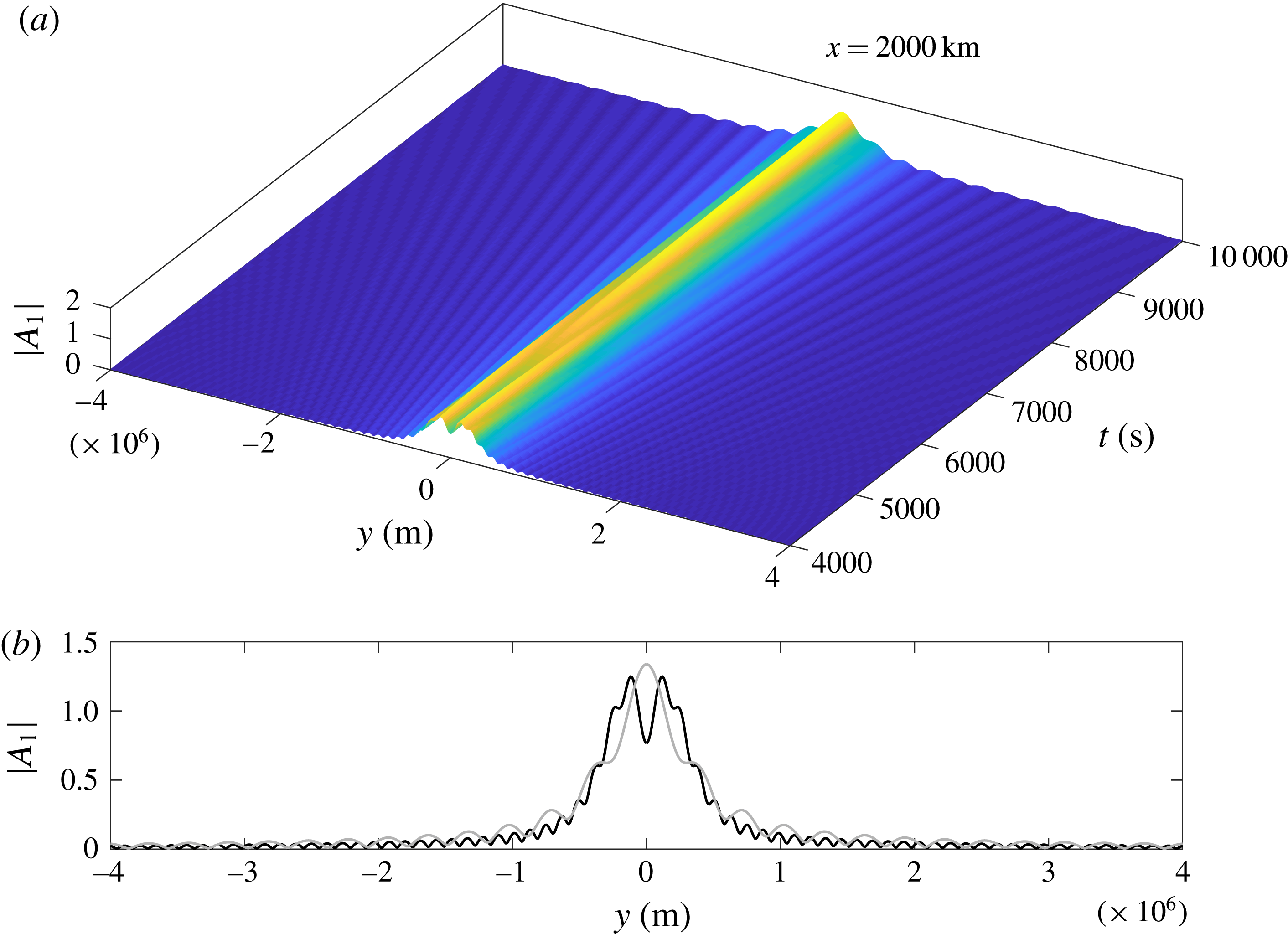
(a) Plot of
 $|A_{1}|$
versus
 $y$
and
 $t$
at
 $x=2000~\text{km}$
. (b) Black and grey curves correspond to
 $t=4000~\text{s}$
and
 $t=10\,000~\text{s}$
, respectively.

(a) Plot of
 $|A_{1}|$
versus
 $y$
and
 $t$
at
 $x=6000~\text{km}$
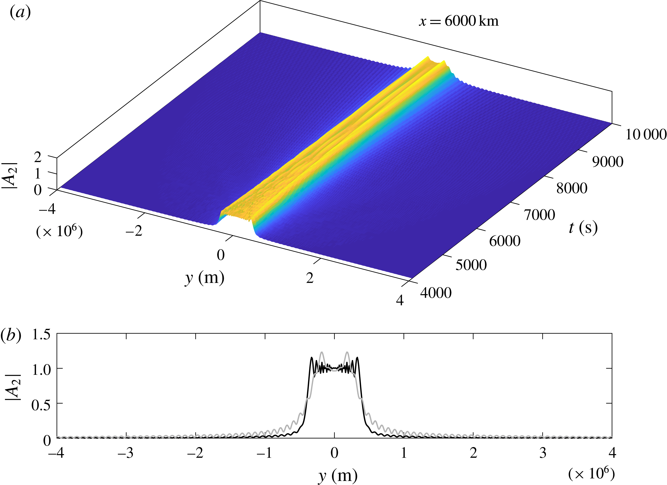
. (b) Black and grey curves correspond to
 $t=4000~\text{s}$
and
 $t=10\,000~\text{s}$
, respectively.

(a) Plot of
 $|A_{2}|$
versus
 $y$
and
 $t$
at
 $x=2000~\text{km}$
. (b) Black and grey curves correspond to
 $t=4000~\text{s}$
and
 $t=10\,000~\text{s}$
, respectively.

(a) Plot of
 $|A_{2}|$
versus
 $y$
and
 $t$
at
 $x=6000~\text{km}$
. (b) Black and grey curves correspond to
 $t=4000~\text{s}$
and
 $t=10\,000~\text{s}$
, respectively.

The envelope
 $|A_{1}(K_{n},X,Y)|$
initially mimics the fault dislocation of top-hat form, but spreads laterally in time (figures 2 and 3). Owing to the properties of the Fresnel integrals,
 $|A_{n}|$
is oscillatory in
 $X$
and
 $Y$
. Moreover, the well-known conservation identity derivable from the Schrödinger equation (4.13),
 $$\begin{eqnarray}\frac{\unicode[STIX]{x2202}}{\unicode[STIX]{x2202}X}\int _{-\infty }^{\infty }|A_{n}|^{2}\,\text{d}Y=0,\end{eqnarray}$$
dictates that lateral decay is compensated by the growth along the centreline. Thus the amplitude
 $|A_{n}|$
near
 $y=0$
can exceed the initial value of 1. In the case of
 $A_{2}$
, the profile at any
 $x$
becomes closer to the top-hat form, as demonstrated in figures 4 and 5. This is because, for finite
 $x/ct$
,
 $K_{2}$
is dominated by
 $\unicode[STIX]{x1D714}_{2}/c=3/2h$
, which is large. This makes
 $X/k_{n}=X/K_{n}$
in (5.2) small and
 $$\begin{eqnarray}\widehat{A}_{n}\approx \frac{\sin \unicode[STIX]{x1D6FC}\ell }{\unicode[STIX]{x1D6FC}},\end{eqnarray}$$
whose inverse transform
 $A_{n}(X,Y)$
is approximately of the initial top-hat profile. As such, higher modes are expected to retain their initial shape for larger distances and longer time. In addition, the evolution may result in temporary local amplification. Note, however, that it can be shown analytically from (5.10) that, for constant
 $x/ct$
(hence
 $K_{n}$
),
 $A_{n}$
vanishes as
 $(X,|Y|)\rightarrow \infty$
.
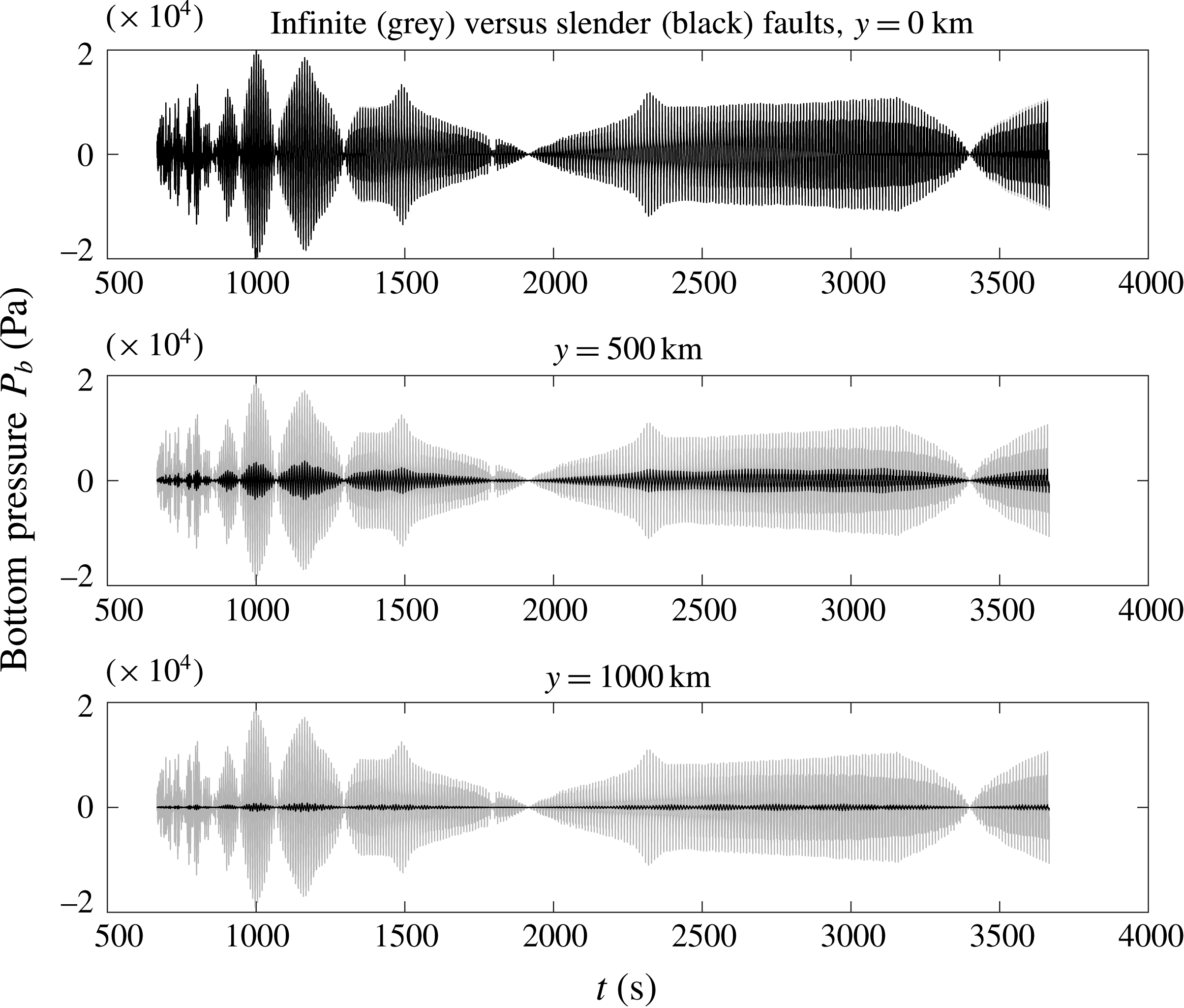
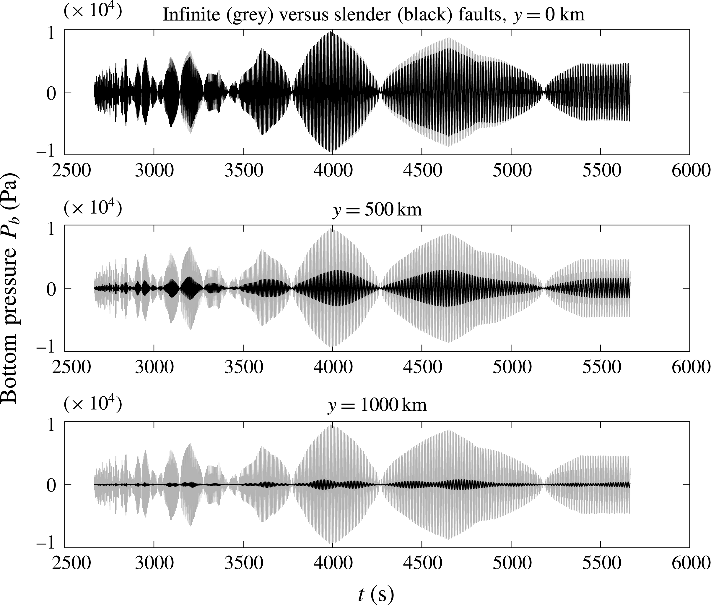
In figures 6 and 7 we show the bottom pressure at different lateral stations along the same lines
 $x=1000~\text{km}$
and
 $x=4000~\text{km}$
. The upward thrust at the fault is assumed to have the speed
 $0.1~\text{m}~\text{s}^{-1}$
. For comparison, the results of an infinitely long fault according to (6.10) and (6.13) with
 $A_{n}=1$
are also shown. At the distance
 $x=1000~\text{km}$
, the pressures at the centreline (
 $y=0$
) by the two theories are virtually the same up to
 $t=3700~\text{s}$
. Significantly lower pressure is evident for the slender fault for all
 $t<3700~\text{s}$
. The difference increases with the distance away from the centreline. At the greater distance of
 $x=4000~\text{km}$
, the drop of the bottom pressure due to the finite fault length is evident after
 $t=4000~\text{s}$
at the centreline station. Away from the centreline, the bottom pressure diminishes even more rapidly for the slender fault.
Variation of bottom pressure in
 $500<t<4000~\text{s}$
at
 $x=1000~\text{ km}$
, for
 $y=0,500,1000~\text{km}$
. Black, slender fault; grey, infinitely long fault.

Variation of bottom pressure in
 $2500<t<6000~\text{s}$
at
 $x=4000~\text{km}$
, for
 $y=0,500,1000~\text{km}$
. Black, slender fault; grey, infinitely long fault.

In a shallower ocean with depth
 $h$
less than
 $4~\text{km}$
, the tsunami advances at a lower speed
 $\sqrt{gh}$
, hence trails behind the acoustic wave front even more. Quantitatively the modal frequencies and modal wavelengths are also reduced. The overall behaviour should remain qualitatively similar.
8 Inverse estimation of fault parameters
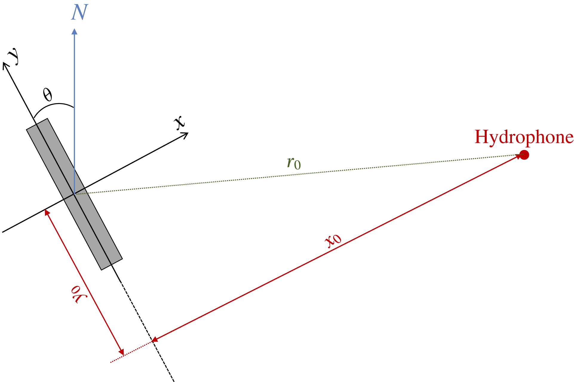
We now extend the inverse approach of Hendin & Stiassnie (Reference Hendin and Stiassnie2013), originally devised for a circular fault, to retrieve the main properties of a slender fault by analysing the pressure recordings available from hydrophones. In particular, we wish to estimate approximately the epicentre coordinates (
 $x_{0},y_{0}$
) relative to one of the hydrophones, orientation relative to the north (see figure 8), fault half-length
 $L$
and half-width
 $b$
, eruption time
 $t_{0}$
(relative to a recorded time
 $\hat{t}$
) and duration
 $T$
. Practically, hydrophone monitoring stations must comprise an array of underwater hydrophones, located at a distance of the order of a kilometre from each other. From wavelet energy entropy considerations and time differences of the arriving signals, the direction (known as bearing) of the epicentre relative to the station can be calculated (see e.g. Wu & Wei Reference Wu and Wei2013). With the bearing at hand, data from a single hydrophone are sufficient to obtain the fault properties, as recently demonstrated by Kadri et al. (Reference Kadri, Crivelli, Parsons, Colbourne and Ryan2017). Although from available seismic sensors the epicentre could be calculated well before the hydro-acoustic signals arrive at the hydrophone station, an alternative estimate can help minimize the uncertainties.
Location and orientation of a slender fault relative to a hydrophone.

8.1 Eruption time and epicentre location and fault orientation
For simplicity, we consider only the first mode
 $n=1$
as in Hendin & Stiassnie (Reference Hendin and Stiassnie2013), and denote quantities obtained from the recordings at the hydrophone by a circumflex. Namely,
 $\widehat{\unicode[STIX]{x1D6FA}}_{\hat{t}_{j}}$
is the measured frequency at the selected instant
 $\hat{t}_{j}$
, where
 $j=1,2,\ldots$
. Now we can rewrite (6.5) in terms of the measured quantities
 $$\begin{eqnarray}\widehat{\unicode[STIX]{x1D6FA}}_{\hat{t}_{j}}=\frac{\unicode[STIX]{x03C0}c}{2h\sqrt{1-[x_{0}/c(\hat{t}_{j}-t_{0})]^{2}}},\quad j=1,2,\ldots ,\end{eqnarray}$$
where
 $t_{0}$
denotes the starting time of eruption. By considering just two different instants
 $\hat{t}_{1}$
and
 $\hat{t}_{2}$
, we can solve for
 $x_{0}$
and
 $t_{0}$
explicitly:
 $$\begin{eqnarray}x_{0}=\frac{(\hat{t}_{2}-\hat{t}_{1})c}{\{1-[\unicode[STIX]{x03C0}c/(2h\widehat{\unicode[STIX]{x1D6FA}}_{\hat{t}_{2}})]^{2}\}^{-1/2}-\{1-[\unicode[STIX]{x03C0}c/(2h\widehat{\unicode[STIX]{x1D6FA}}_{\hat{t}_{1}})]^{2}\}^{-1/2}}\end{eqnarray}$$
and
 $$\begin{eqnarray}t_{0}=\hat{t}_{j}-\frac{x_{0}}{c}\left\{1-\left[\frac{\unicode[STIX]{x03C0}c}{2h\widehat{\unicode[STIX]{x1D6FA}}_{\hat{t}_{j}}}\right]^{2}\right\}^{-1/2},\quad j=1\text{ or }2.\end{eqnarray}$$
If (
 $x_{0},y_{0}$
) is known from seismic recordings,
 $t_{0}$
is found at once from (8.3). Otherwise
 $x_{0}$
can be calculated from hydrophone records according to (8.2), and then
 $t_{0}$
from (8.3). If only the distance
 $r_{0}$
between the epicentre and hydrophone is known from the seismic recordings, the calculated
 $x_{0}$
can be used to get
 $y_{0}=\sqrt{r_{0}^{2}-x_{0}^{2}}$
. For simplicity this is assumed in the present example, with the prescribed value
 $r_{0}=10\,000~\text{km}$
. If seismic information is not available at all,
 $y_{0}$
can be estimated by employing the acoustic recordings of the pressure amplitude together with the remaining parameters, as noted at the end of § 8.2.
Once
 $(x_{0},y_{0})$
is found, the orientation of the slender fault relative to the north
 $\unicode[STIX]{x1D703}$
can be calculated from figure 8,
 $$\begin{eqnarray}\unicode[STIX]{x1D703}=90^{\circ }-\tan ^{-1}(x_{0}/y_{0}).\end{eqnarray}$$
For the prescribed distance from the fault centre to the hydrophone
 $r_{0}=10\,000~\text{km}$
, we find
 $x_{0}=9994~\text{km}$
,
 $y_{0}=341~\text{km}$
,
 $\unicode[STIX]{x1D703}=1.95^{\circ }$
and
 $t_{0}=5.739~\text{s}$
.
8.2 Fault length, width, duration and rising speed
Finally, we employ (6.13) for
 $n=1$
only to approximate the measured bottom pressure
 $$\begin{eqnarray}\widehat{P}_{1}(\hat{t}_{j})=\unicode[STIX]{x1D70C}W_{0}|A_{1}(K_{1},X,Y)|\frac{2^{7/2}C}{\sqrt{\unicode[STIX]{x03C0}^{3}x_{0}k(\widehat{\unicode[STIX]{x1D6FA}}_{\hat{t}_{j}})}}\sin [k(\widehat{\unicode[STIX]{x1D6FA}}_{\hat{t}_{j}})b]\sin (\widehat{\unicode[STIX]{x1D6FA}}_{\hat{t}_{j}}T).\end{eqnarray}$$
With
 $y_{0}$
known, four unknowns remain:
 $L,b,W_{0},T$
. Choosing four different time instants
 $\hat{t}_{j},~j=1,2,3,4$
, we get four calculated
 $\widehat{P}_{1}(\hat{t}_{j})$
, which are taken as the measured amplitudes. Since
 $\widehat{P}_{1}(\hat{t}_{j})$
is a function of
 $W_{0},b,T$
and
 $L$
through
 $|A_{1}|$
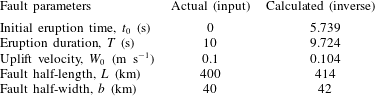
, these four amplitudes comprise four algebraic equations for the four unknowns, and are solved numerically. In table 2 the direct input and calculated fault parameters are compared for the case in § 7. Better accuracy is possible by more elaborate computations using more modes. If
 $r_{0}$
is not known from seismic records, one can evaluate
 $\widehat{P}_{1}$
at another time instant
 $\hat{t}_{5}$
to get an additional equation, and then solve for
 $y_{1}$
and the four other parameters from five equations.
Fault parameters for the case studied in § 7.
9 Conclusion
Making use of the sharp difference between the speeds of sound and of gravity waves, we have developed a simple analytical theory based on linearized acoustics excluding the gravity wave effect. By further focusing on slender faults, which are quite common in nature, an explicit theory is worked out by employing the asymptotic method of multiple scales. The effects of two-dimensional trans-ocean propagation are worked out for large time and long distances. By following the approximate approach of Hendin & Stiassnie (Reference Hendin and Stiassnie2013), we have demonstrated that our direct theory facilitates the inverse estimates of fault properties (location, dimension, duration, orientation, etc.) from pressure measurements at one hydrophone. For helping the design of acoustic sensing systems for early warning of tsunamis, it is necessary to account for the scattering of sound by wind-induced surface waves, coastline geometry, seabed topography and dissipation in water and along the seabed, etc. We hope that the present asymptotic approach can be extended to expedite practical computational modelling.
Appendix A. Inverse transform of
$I$

We rewrite (3.7) as
 $$\begin{eqnarray}\displaystyle \displaystyle \unicode[STIX]{x1D719}_{0} & = & \displaystyle -\frac{W_{0}}{2\unicode[STIX]{x03C0}2\unicode[STIX]{x03C0}}\int _{-\infty }^{\infty }\,\text{d}\unicode[STIX]{x1D714}\,\text{e}^{-\text{i}\unicode[STIX]{x1D714}t}\int _{-\infty }^{\infty }\,\text{d}k\,\text{e}^{\text{i}kx}\frac{G}{\unicode[STIX]{x1D707}}\frac{\sin \unicode[STIX]{x1D707}(h-z)}{\cos \unicode[STIX]{x1D707}h}\nonumber\\ \displaystyle & = & \displaystyle -\frac{W_{0}}{2\unicode[STIX]{x03C0}}\int _{-\infty }^{\infty }\text{i}\,\text{d}\unicode[STIX]{x1D714}\,\text{e}^{-\text{i}\unicode[STIX]{x1D714}t}\left\{\frac{1}{2\unicode[STIX]{x03C0}\text{i}}\int _{-\infty }^{\infty }\,\text{d}k\,\text{e}^{\text{i}kx}\frac{G}{\unicode[STIX]{x1D707}}\frac{\sin \unicode[STIX]{x1D707}(h-z)}{\cos \unicode[STIX]{x1D707}h}\right\}\nonumber\\ \displaystyle & = & \displaystyle -\frac{W_{0}}{2\unicode[STIX]{x03C0}}\int _{-\infty }^{\infty }\text{i}\,\text{d}\unicode[STIX]{x1D714}\,\text{e}^{-\text{i}\unicode[STIX]{x1D714}t}I(x,z,\unicode[STIX]{x1D714}),\end{eqnarray}$$
where
 $I$
is the
 $k$
integral
 $$\begin{eqnarray}I(x,z,\unicode[STIX]{x1D714})=\frac{1}{2\unicode[STIX]{x03C0}\text{i}}\int _{-\infty }^{\infty }\,\text{d}k\,\text{e}^{\text{i}kx}\frac{G}{\unicode[STIX]{x1D707}}\frac{\sin \unicode[STIX]{x1D707}(h-z)}{\cos \unicode[STIX]{x1D707}h}.\end{eqnarray}$$
The integrand has poles at the zeros of
 $\cos \unicode[STIX]{x1D707}h$
:
 $$\begin{eqnarray}\cos \unicode[STIX]{x1D707}h=0,\quad \unicode[STIX]{x1D707}=\pm \unicode[STIX]{x1D707}_{n}=\pm \left(n-\frac{1}{2}\right)\frac{\unicode[STIX]{x03C0}}{h},\quad \unicode[STIX]{x1D707}_{1}<\unicode[STIX]{x1D707}_{2}<\unicode[STIX]{x1D707}_{3}<\cdots \,.\end{eqnarray}$$
To facilitate the indentation of the path of integration in the complex
 $k$
-plane, we apply the method of Rayleigh damping and replace
 $\unicode[STIX]{x1D714}$
by
 $\unicode[STIX]{x1D714}^{\prime }=\unicode[STIX]{x1D714}+\text{i}\unicode[STIX]{x1D6FF}^{\prime }$
, where
 $\unicode[STIX]{x1D6FF}^{\prime }>0$
is a small and positive number, which will be set to zero in the limit. Thus
 $$\begin{eqnarray}\displaystyle & \displaystyle \unicode[STIX]{x1D707}=\sqrt{\frac{{\unicode[STIX]{x1D714}^{\prime }}^{2}}{c^{2}}-k^{2}}, & \displaystyle\end{eqnarray}$$
 $$\begin{eqnarray}\displaystyle & \displaystyle k=\pm \sqrt{\frac{{\unicode[STIX]{x1D714}^{\prime }}^{2}}{c^{2}}-\unicode[STIX]{x1D707}^{2}}. & \displaystyle\end{eqnarray}$$
We define
 $\unicode[STIX]{x1D714}_{n}$
by
 $$\begin{eqnarray}\unicode[STIX]{x1D707}_{n}=\left(n-\frac{1}{2}\right)\frac{\unicode[STIX]{x03C0}}{h}\,\equiv \,\frac{\unicode[STIX]{x1D714}_{n}}{c},\end{eqnarray}$$
and consider the following two possibilities. (i) If
 $\unicode[STIX]{x1D714}^{2}>\unicode[STIX]{x1D714}_{N}^{2}$
,
 $2N$
complex poles,
 $$\begin{eqnarray}k=\pm k_{n}^{\prime },\quad n=1,2,3,\ldots ,N,\end{eqnarray}$$
exist in the
 $k$
-plane, where
 $$\begin{eqnarray}k_{n}^{\prime }=\frac{\sqrt{(\unicode[STIX]{x1D714}+\text{i}\unicode[STIX]{x1D6FF}^{\prime })^{2}-\unicode[STIX]{x1D714}_{n}^{2}}}{c}\approx k_{n}+\text{i}\frac{\unicode[STIX]{x1D6FF}\unicode[STIX]{x1D714}}{c^{2}(\unicode[STIX]{x1D714}^{2}-\unicode[STIX]{x1D714}_{n}^{2})},\end{eqnarray}$$
with
 $k_{1}>k_{2}>\cdots >k_{N}$
. Because of the Rayleigh damping factor
 $\unicode[STIX]{x1D707}$
,
 $+k_{n}^{\prime }$
is slightly above the real
 $k$
axis (the path of integration) if
 $\unicode[STIX]{x1D714}>0$
, and slightly below the real axis if
 $\unicode[STIX]{x1D714}<0$
. On the other hand,
 $-k_{n}^{\prime }$
is slightly below the real
 $k$
axis if
 $\unicode[STIX]{x1D714}>0$
, and slightly above the real axis if
 $\unicode[STIX]{x1D714}<0$
. (ii) If
 $\unicode[STIX]{x1D714}^{2}<\unicode[STIX]{x1D714}_{N}^{2}$
,
 $2\times \infty$
imaginary poles exist in the
 $k$
-plane,
 $$\begin{eqnarray}k=\pm \text{i}\unicode[STIX]{x1D706}_{n},\quad n=N+1,N+2,\ldots ,\quad \unicode[STIX]{x1D706}_{N+1}<\unicode[STIX]{x1D706}_{N+2}<\cdots \,,\quad \text{if}~\unicode[STIX]{x1D714}^{2}<\unicode[STIX]{x1D714}_{N}^{2},\end{eqnarray}$$
where
 $$\begin{eqnarray}\unicode[STIX]{x1D706}_{n}=\frac{\sqrt{\unicode[STIX]{x1D714}_{n}^{2}-\unicode[STIX]{x1D714}^{2}}}{C}.\end{eqnarray}$$
Let us first break the
 $\unicode[STIX]{x1D714}$
integral in (A 1):
 $$\begin{eqnarray}\displaystyle \unicode[STIX]{x1D719}_{0} & = & \displaystyle -\frac{W_{0}}{2\unicode[STIX]{x03C0}}\left\{\int _{-\infty }^{-\unicode[STIX]{x1D714}_{N}}+\int _{\unicode[STIX]{x1D714}_{N}}^{\infty }\right\}\text{i}\,\text{d}\unicode[STIX]{x1D714}\,\text{e}^{-\text{i}\unicode[STIX]{x1D714}t}\left\{\frac{1}{2\unicode[STIX]{x03C0}\text{i}}\int _{-\infty }^{\infty }\,\text{d}k\,\text{e}^{\text{i}kx}\frac{G}{\unicode[STIX]{x1D707}}\frac{\sin \unicode[STIX]{x1D707}(h-z)}{\cos \unicode[STIX]{x1D707}h}\right\}\nonumber\\ \displaystyle & & \displaystyle \displaystyle -\,\frac{W_{0}}{2\unicode[STIX]{x03C0}}\left\{\int _{-\unicode[STIX]{x1D714}_{N}}^{\unicode[STIX]{x1D714}_{N}}\right\}\text{i}\,\text{d}\unicode[STIX]{x1D714}\,\text{e}^{-\text{i}\unicode[STIX]{x1D714}t}\left\{\frac{1}{2\unicode[STIX]{x03C0}\text{i}}\int _{-\infty }^{\infty }\,\text{d}k\,\text{e}^{\text{i}kx}\frac{G}{\unicode[STIX]{x1D707}}\frac{\sin \unicode[STIX]{x1D707}(h-z)}{\cos \unicode[STIX]{x1D707}h}\right\}\nonumber\\ \displaystyle & = & \displaystyle -\,\frac{W_{0}}{2\unicode[STIX]{x03C0}}\left\{\int _{-\infty }^{-\unicode[STIX]{x1D714}_{N}}+\int _{\unicode[STIX]{x1D714}_{N}}^{\infty }\right\}\text{i}\,\text{d}\unicode[STIX]{x1D714}\,\text{e}^{-\text{i}\unicode[STIX]{x1D714}t}I(x,z,\unicode[STIX]{x1D714})-\frac{1}{2\unicode[STIX]{x03C0}}\left\{\int _{-\unicode[STIX]{x1D714}_{N}}^{\unicode[STIX]{x1D714}_{N}}\right\}\text{i}\,\text{d}\unicode[STIX]{x1D714}\,\text{e}^{-\text{i}\unicode[STIX]{x1D714}t}I(x,z,\unicode[STIX]{x1D714})\nonumber\\ \displaystyle & = & \displaystyle -\frac{W_{0}}{2\unicode[STIX]{x03C0}}\left(I_{+}+I_{-}+I_{e}\right),\end{eqnarray}$$
where
 $$\begin{eqnarray}\left(I_{+},I_{-},I_{e}\right)=\left(\int _{\unicode[STIX]{x1D714}_{N}}^{\infty },\int _{-\infty }^{-\unicode[STIX]{x1D714}_{N}},\int _{-\unicode[STIX]{x1D714}_{N}}^{\unicode[STIX]{x1D714}_{N}}\right)\text{i}\,\text{d}\unicode[STIX]{x1D714}\,\text{e}^{-\text{i}\unicode[STIX]{x1D714}t}I(x,z,\unicode[STIX]{x1D714}).\end{eqnarray}$$
Next, we take the limit
 $\unicode[STIX]{x1D6FF}^{\prime }\rightarrow 0+$
. For
 $I_{+}$
we indent the path of
 $k$
integration below the poles
 $k_{n}^{\prime }$
on the positive real side of the
 $k$
-plane and above the poles
 $-k_{n}^{\prime }$
on the negative real side of the
 $k$
-plane. The anticlockwise contour is closed by a large semicircle in the upper
 $k$
-plane. We get from the residues
 $$\begin{eqnarray}I_{+}=\mathop{\sum }_{n=1}^{N}\frac{G(k_{n}^{\prime })}{\unicode[STIX]{x1D707}_{n}}\displaystyle \frac{\sin \unicode[STIX]{x1D707}_{n}(h-z)}{\left.\displaystyle \frac{\unicode[STIX]{x2202}\cos \unicode[STIX]{x1D707}h}{\unicode[STIX]{x2202}k}\right|_{k_{n}^{\prime }}}\text{e}^{\text{i}k_{n}^{\prime }|x|}=\mathop{\sum }_{1}^{N}\frac{G(k_{n})}{k_{n}h}\frac{\sin \unicode[STIX]{x1D707}_{n}(h-z)}{\sin \unicode[STIX]{x1D707}_{n}h}\text{e}^{\text{i}k_{n}|x|},\end{eqnarray}$$
which gives outgoing waves with
 $\text{e}^{-\text{i}\unicode[STIX]{x1D714}t}$
.
For
 $I_{-}$
we indent the path below
 $-k_{n}^{\prime }$
on the negative real side of the
 $k$
-plane and above
 $k_{n}^{\prime }$
. By closing the indented path by an anticlockwise contour of a semicircle in the upper
 $k$
-plane, we get from all
 $-k_{n}^{\prime }$
the residues
 $$\begin{eqnarray}I_{-}=\mathop{\sum }_{1}^{N}\frac{G(-k_{n})}{-k_{n}h}\frac{\sin \unicode[STIX]{x1D707}_{n}(h-z)}{\sin \unicode[STIX]{x1D707}_{n}h}\text{e}^{-\text{i}k_{n}|x|}=-\mathop{\sum }_{1}^{N}\frac{G(k_{n})}{k_{n}h}\frac{\sin \unicode[STIX]{x1D707}_{n}(h-z)}{\sin \unicode[STIX]{x1D707}_{n}h}\text{e}^{-\text{i}k_{n}|x|},\end{eqnarray}$$
which gives outgoing waves with
 $\text{e}^{\text{i}\unicode[STIX]{x1D714}t}$
. Use is made of
 $G(-k_{n})/(-k_{n})=-G(k_{n})/k_{n}$
.
Finally for
 $I_{e}$
we close the anticlockwise contour in the upper half
 $k$
-plane. From the positive imaginary poles, we get
 $$\begin{eqnarray}I_{e}=\mathop{\sum }_{N+1}^{\infty }\frac{G(\text{i}\unicode[STIX]{x1D706}_{n})}{\text{i}\unicode[STIX]{x1D706}_{n}h}\frac{\sin \unicode[STIX]{x1D707}_{n}(h-z)}{\sin \unicode[STIX]{x1D707}_{n}h}\text{e}^{-\unicode[STIX]{x1D706}_{n}|x|},\end{eqnarray}$$
where
 $$\begin{eqnarray}\frac{G(\text{i}\unicode[STIX]{x1D706}_{n})}{\text{i}\unicode[STIX]{x1D706}_{n}h}=\frac{4\sin \text{i}\unicode[STIX]{x1D706}_{n}b\,\sin \unicode[STIX]{x1D714}T}{\text{i}\unicode[STIX]{x1D706}_{n}h\,\unicode[STIX]{x1D714}\text{i}\unicode[STIX]{x1D706}_{n}h}=\frac{4\sinh \unicode[STIX]{x1D706}_{n}b\,\sin \unicode[STIX]{x1D714}T}{\unicode[STIX]{x1D706}_{n}h\,\unicode[STIX]{x1D714}\text{i}\unicode[STIX]{x1D706}_{n}h}=\text{imaginary},\end{eqnarray}$$
and
 $I_{e}$
represents the evanescent modes.
In summary
 $$\begin{eqnarray}\displaystyle \displaystyle \unicode[STIX]{x1D719}_{0} & = & \displaystyle -\frac{W_{0}}{2\unicode[STIX]{x03C0}}\left\{\int _{\unicode[STIX]{x1D714}_{N}}^{\infty }\text{i}\,\text{d}\unicode[STIX]{x1D714}\,\text{e}^{-\text{i}\unicode[STIX]{x1D714}t}\mathop{\sum }_{1}^{N}\frac{G(k_{n})}{k_{n}h}\frac{\sin \unicode[STIX]{x1D707}_{n}(h-z)}{\sin \unicode[STIX]{x1D707}_{n}h}\text{e}^{\text{i}k_{n}|x|}\right.\nonumber\\ \displaystyle & & \displaystyle \displaystyle \left.-\,\int _{-\infty }^{-\unicode[STIX]{x1D714}_{N}}\text{i}\,\text{d}\unicode[STIX]{x1D714}\,\text{e}^{-\text{i}\unicode[STIX]{x1D714}t}\mathop{\sum }_{1}^{N}\frac{G(k_{n})}{k_{n}h}\frac{\sin \unicode[STIX]{x1D707}_{n}(h-z)}{\sin \unicode[STIX]{x1D707}_{n}h}\text{e}^{-\text{i}k_{n}|x|}\right\}\nonumber\\ \displaystyle & & \displaystyle \displaystyle -\,\frac{W_{0}}{2\unicode[STIX]{x03C0}}\left[\int _{-\unicode[STIX]{x1D714}_{N}}^{0}+\int _{0}^{\unicode[STIX]{x1D714}_{N}}\right]\text{i}\,\text{d}\unicode[STIX]{x1D714}\,\text{e}^{-\text{i}\unicode[STIX]{x1D714}t}\mathop{\sum }_{N+1}^{\infty }\frac{G(\text{i}\unicode[STIX]{x1D706}_{n})}{\text{i}\unicode[STIX]{x1D706}_{n}h}\frac{\sin \unicode[STIX]{x1D707}_{n}(h-z)}{\sin \unicode[STIX]{x1D707}_{n}h}\text{e}^{-\unicode[STIX]{x1D706}_{n}|x|},\end{eqnarray}$$
which can be further simplified to
 $$\begin{eqnarray}\displaystyle \unicode[STIX]{x1D719}_{0} & = & \displaystyle -\frac{W_{0}}{\unicode[STIX]{x03C0}}\,\text{Re}\int _{\unicode[STIX]{x1D714}_{N}}^{\infty }\text{i}\,\text{d}\unicode[STIX]{x1D714}\,\text{e}^{-\text{i}\unicode[STIX]{x1D714}t}\mathop{\sum }_{1}^{N}\frac{G(k_{n},\unicode[STIX]{x1D714})}{k_{n}h}\frac{\sin \unicode[STIX]{x1D707}_{n}(h-z)}{\sin \unicode[STIX]{x1D707}_{n}h}\text{e}^{\text{i}k_{n}|x|}\nonumber\\ \displaystyle & & \displaystyle -\,\displaystyle \frac{W_{0}}{\unicode[STIX]{x03C0}}\int _{0}^{\unicode[STIX]{x1D714}_{N}}\,\text{d}\unicode[STIX]{x1D714}\cos (\unicode[STIX]{x1D714}t)\mathop{\sum }_{N+1}^{\infty }\frac{G(\unicode[STIX]{x1D706}_{n},\unicode[STIX]{x1D714})}{\unicode[STIX]{x1D706}_{n}h}\frac{\sin \unicode[STIX]{x1D707}_{n}(h-z)}{\sin \unicode[STIX]{x1D707}_{n}h}\text{e}^{-\unicode[STIX]{x1D706}_{n}|x|}.\end{eqnarray}$$
The bottom pressure is
 $$\begin{eqnarray}\displaystyle p & = & \displaystyle \left.-\unicode[STIX]{x1D70C}\frac{\unicode[STIX]{x2202}\unicode[STIX]{x1D719}_{0}}{\unicode[STIX]{x2202}t}\right|_{z=0}=-\frac{W_{0}}{\unicode[STIX]{x03C0}}\,\text{Re}\int _{\unicode[STIX]{x1D714}_{N}}^{\infty }\unicode[STIX]{x1D714}\,\text{d}\unicode[STIX]{x1D714}\,\text{e}^{-\text{i}\unicode[STIX]{x1D714}t}\mathop{\sum }_{1}^{N}\frac{G(k_{n},\unicode[STIX]{x1D714})}{k_{n}h}\text{e}^{\text{i}k_{n}|x|}\nonumber\\ \displaystyle & & \displaystyle +\,\frac{W_{0}}{\unicode[STIX]{x03C0}}\int _{0}^{\unicode[STIX]{x1D714}_{N}}\unicode[STIX]{x1D714}\,\text{d}\unicode[STIX]{x1D714}\sin (\unicode[STIX]{x1D714}t)\mathop{\sum }_{N+1}^{\infty }\frac{G(\unicode[STIX]{x1D706}_{n},\unicode[STIX]{x1D714})}{\unicode[STIX]{x1D706}_{n}h}\text{e}^{-\unicode[STIX]{x1D706}_{n}|x|}.\end{eqnarray}$$
Appendix B. Envelope equation for slowly varying sea depth
Let the uneven sea depth
 $H$
change very slowly in both horizontal directions according to
 $H(X,y_{2})$
where
 $X=\unicode[STIX]{x1D716}^{2}x$
and
 $y_{2}=\unicode[STIX]{x1D716}^{2}y$
. By switching the coordinate system from
 $x,y,z$
to
 $x,y,z^{\prime }$
, the sea layer becomes
 $-H(X,y_{2})<z^{\prime }<0$
. The leading-order results in §§ 3 and 4 and appendix A remain valid if
 $h$
is replaced by
 $H$
and
 $h-z$
by
 $z^{\prime }$
. Now (2.13) must be replaced by
 $$\begin{eqnarray}\frac{\unicode[STIX]{x2202}\unicode[STIX]{x1D719}_{2}}{\unicode[STIX]{x2202}z^{\prime }}=-\frac{\unicode[STIX]{x2202}H}{\unicode[STIX]{x2202}X}\frac{\unicode[STIX]{x2202}\unicode[STIX]{x1D719}_{0}}{\unicode[STIX]{x2202}x},\quad z^{\prime }=-H.\end{eqnarray}$$
Since
 $\unicode[STIX]{x2202}\unicode[STIX]{x1D719}_{0}/\unicode[STIX]{x2202}y=0$
, the term
 $(\unicode[STIX]{x2202}H/\unicode[STIX]{x2202}y_{2})(\unicode[STIX]{x2202}\unicode[STIX]{x1D719}_{0}/\unicode[STIX]{x2202}y)=0$
. The
 $y_{2}$
dependence of
 $H$
does not enter the seabed boundary condition explicitly up to the present order. Finally solvability of the order
 $O(\unicode[STIX]{x1D716}^{2})$
problem leads to the envelope equation
 $$\begin{eqnarray}2\text{i}k_{n}\frac{\unicode[STIX]{x2202}A_{n}}{\unicode[STIX]{x2202}X}+\text{i}(2k_{n}\sin ^{2}\unicode[STIX]{x1D707}_{n}H)\left(\frac{1}{H}\frac{\unicode[STIX]{x2202}H}{\unicode[STIX]{x2202}X}\right)A_{n}+\frac{\unicode[STIX]{x2202}^{2}A_{n}}{\unicode[STIX]{x2202}Y^{2}}=0.\end{eqnarray}$$
For given
 $H(X,y_{2})$
, this modified Schrödinger equation can be conveniently solved by any numerical method for the diffusion equation.