



1. Introduction
Gamma-ray binaries are an important class of high-energy astrophysical sources (Guillaume Dubus Reference Dubus2013). A canonical example is LS 5039, which has historically been the subject of intense multiwavelength campaigns (Hadasch et al. Reference Hadasch2012; Collmar & Zhang Reference Collmar and Zhang2014) (other sources include (LS I +61
 ${}^{\circ} $
303, HESS J0632+057, 1FGL J1018.6-5856, and 1FGL J1018.6-5856).
In these sources, the relativistic pulsar wind interacts with the wind of the companion and later with the interstellar matter. In the process, ultra-relativistic particles are accelerated and emit radio emission to gamma-rays (see, e.g. Tavani & Arons Reference Tavani and Arons1997; Sierpowska & Bednarek Reference Sierpowska and Bednarek2005; Dubus Reference Dubus2006; Khangulyan et al. Reference Khangulyan, Hnatic, Aharonian and Bogovalov2007; Kong, Cheng, & Huang Reference Kong, Cheng and Huang2012; Zabalza et al. Reference Zabalza, Bosch-Ramon, Aharonian and Khangulyan2013; Dubus, Lamberts, & Fromang Reference Dubus, Lamberts and Fromang2015; Molina & Bosch-Ramon Reference Molina and Bosch-Ramon2020; Huber, Kissmann, & Reimer Reference Huber, Kissmann and Reimer2021; Khangulyan, Barkov, & Popov Reference Khangulyan, Barkov and Popov2022; Lopez-Miralles et al. Reference Lopez-Miralles, Perucho, Marti, Migliari and Bosch-Ramon2022). The accretion black hole as a compact object was also discussed in the literature (see Casares et al. Reference Casares, Ribo, Ribas, Paredes, Marti and Herrero2005; Bosch-Ramon & Khangulyan Reference Bosch-Ramon and Khangulyan2009; Barkov & Khangulyan Reference Barkov and Khangulyan2012), but it looks less feasible due to the strict energetic constraint observed in the MeV energy range (Collmar & Zhang Reference Collmar and Zhang2014).
Importantly, the interaction of the wind from the neutron star with the wind from a high-mass companion leads to the orbital-dependent X-ray emission and gamma-ray emission. Often flares are observed at particular orbital phases (e.g. Abdo et al. Reference Abdo2011). Understanding the origin and properties of this orbital dependence is the main goal of the present work.
There is general agreement that this complex behaviour is the result of the wind–wind interaction between the relativistic highly magnetised wind of neutron star and a powerful (and anisotropic) wind from the main sequence companion (Guillaume Dubus Reference Dubus2013), the main mechanisms of the non-thermal emission are synchrotron (SYN) and inverse-Compton (IC) (see Bosch-Ramon & Khangulyan Reference Bosch-Ramon and Khangulyan2009), but the details of the interaction and production of γ-ray emission remain controversial.
Here, we point out that the wind–wind interaction depends both on the global properties of the pulsar (its spin-down power) and of the companion’s wind (mass and momentum loss rates), as well on the more subtle geometrical properties: relative direction of the pulsar’s rotational axis and its magnetic inclination, and orbital-dependent direction from the pulsar to the companion. In addition, since effects of relativistic beaming are likely to be important, the view of the interacting region depends on the orbital-dependent line of sight. This requires both 3D simulations, as well as investigation of various parameters.
The system resembles the case of the pulsar–ISM interaction studied by Barkov, Lyutikov, & Khangulyan (Reference Barkov, Lyutikov and Khangulyan2019a), but is also different in many ways. In the case of pulsar–ISM interaction we can identify two basic geometric types depending on the relative orientation of the pulsar rotational axis and the velocity: (i) a ‘Rifle Bullet’, with the pulsar spin and velocity aligned and (ii) a ‘Frisbee’, with the pulsar spin and velocity orthogonal to each other. The internal dynamics of the shocked pulsar wind is considerably different in these cases. The ‘Frisbee’ configuration results in substantially non-symmetric morphologies of the tail region due to the influence of the internal hoop stresses.
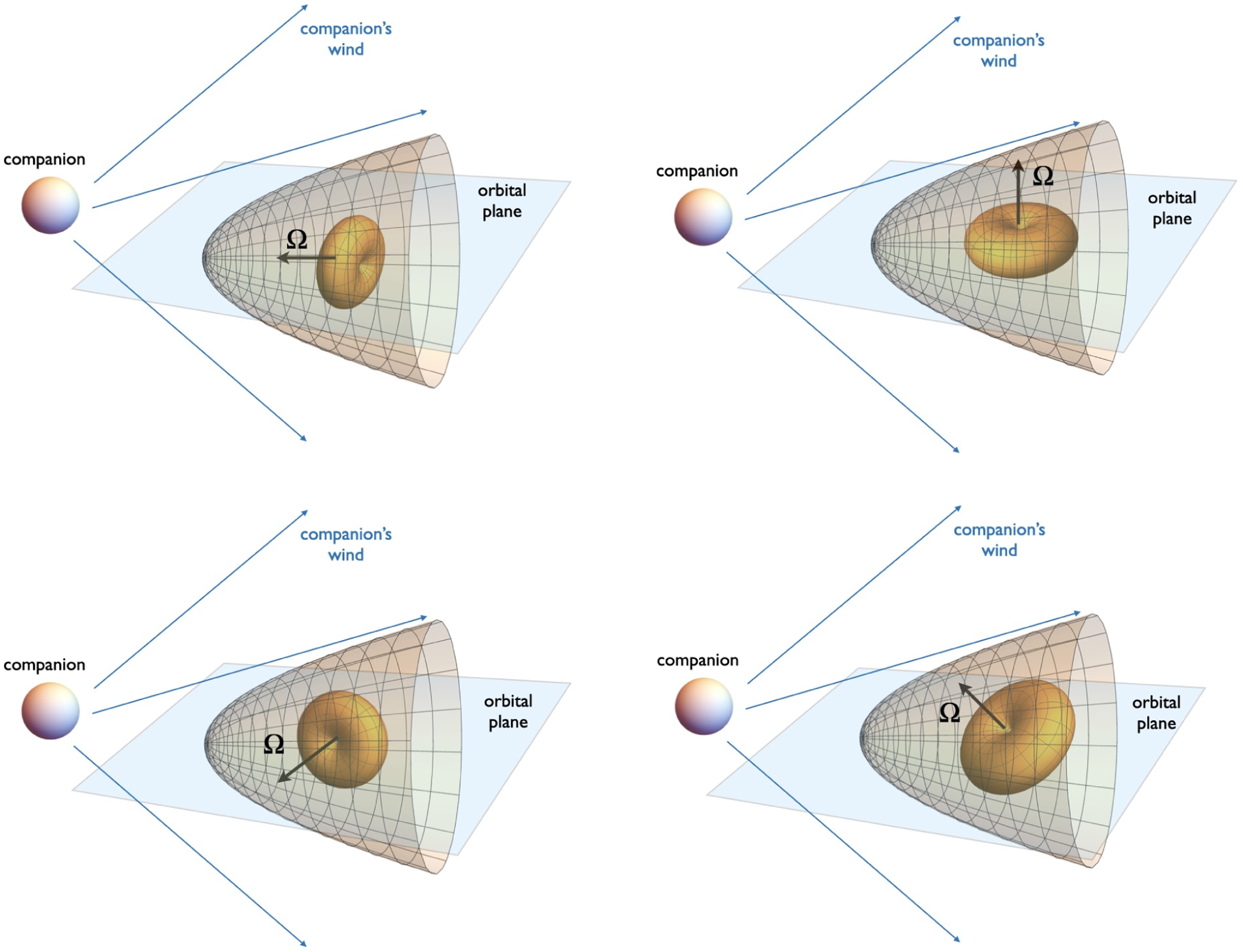
Somewhat similar configurations are expected in the binary case, Fig. 1. One difference of the wind–wind interaction from the wind–ISM case is that the relative geometry is orbital phase-dependent (except for ‘Frisbee’ configuration). For the case of spin in the plane of the orbit, the system evolves from the ‘Bullet’ to the ‘Cartwheel’ configuration every quarter of the period.
Basic geometries: ‘Rifle Bullet’ (the spin of the neutron star is in the orbital plane, directed towards the companion, top left panel), ‘Frisbee’ (with the spin of the neutron star perpendicular both to the orbital plane, top right panel), ‘Cartwheel’ (spin of the neutron star in the orbital plane but perpendicular to the direction to the companion, bottom left panel), and a mixed ‘Frisbee-Bullet’ configuration (bottom right panel). The central doughnut-like structure indicates the distribution of wind power.
The most important difference between the wind–ISM and wind–wind interaction is the tail structure of the resulting pulsar wind nebulae (PWN). First, the winds’ collision creates two shocks separated by contact discontinuity (CD). The shock in the normal star wind we call the forward shock (FS) and the second one in the pulsar wind we call the reverse shock (RS), Fig. 2. In the wind–ISM case, the tailward pulsar wind always terminates at the so-called Mach disc – a strong, nearly perpendicular shock (perpendicular in a sense that flow velocity is nearly orthogonal to the shock plane Barkov et al. Reference Barkov, Lyutikov, Klingler and Bordas2019b). In the wind–wind case ‘open’ structure has a possibility of creating – when the weaker wind extends as a supersonic flow to infinity in the tailward direction, see Fig. 2 left panel and Fig. 10 of Bogovalov et al. Reference Bogovalov, Khangulyan, Koldoba, Ustyugova and Aharonian2008. In such a case, the confined pulsar wind expands conically, keeping the force balance with the confining wind.
Two possible structures of the tail flow: ‘open’ one, when the supersonic pulsar wind partially extends to infinity, and ‘closed’ one, when the supersonic pulsar wind always terminates at the reverse shock. For a given thrust ratio η the type of configuration also depends on the neutron star geometry, see Fig. 3. In the case pulsar–ISM interaction only closed configurations are possible. For ‘Stellar wind’–‘pulsar wind’ case switching between the two morphologies leads to sudden changes in the resulting emission.

Conventionally, in a fluid description (Bogovalov et al. Reference Bogovalov, Khangulyan, Koldoba, Ustyugova and Aharonian2008), the key parameter of the interaction of winds is momentum thrust ratio
 $\eta $
which in the case of pulsar and stellar wind interaction is
 \begin{align}\eta = \frac{{{L_{sd}}}}{{\dot M{v_w}c}},\end{align}
here
 $\dot M$
and
 ${v_w}$
are stellar wind mass loss rate and speed correspondingly, c is speed of light, and
 ${L_{sd}}$
is pulsar spindown power. For sufficiently small
 $\eta \le 0.01$
the Mach disc appears at large distances down the pulsar tail (see Fig. 2 right panel), of the order of the orbital separation, and moves to shorter distances if we reduce
 $\eta $
. Thus, we expect a sensitive dependence of the overall morphology, and consequently of the emission properties, on the momentum thrust ratio
 $\eta $
.
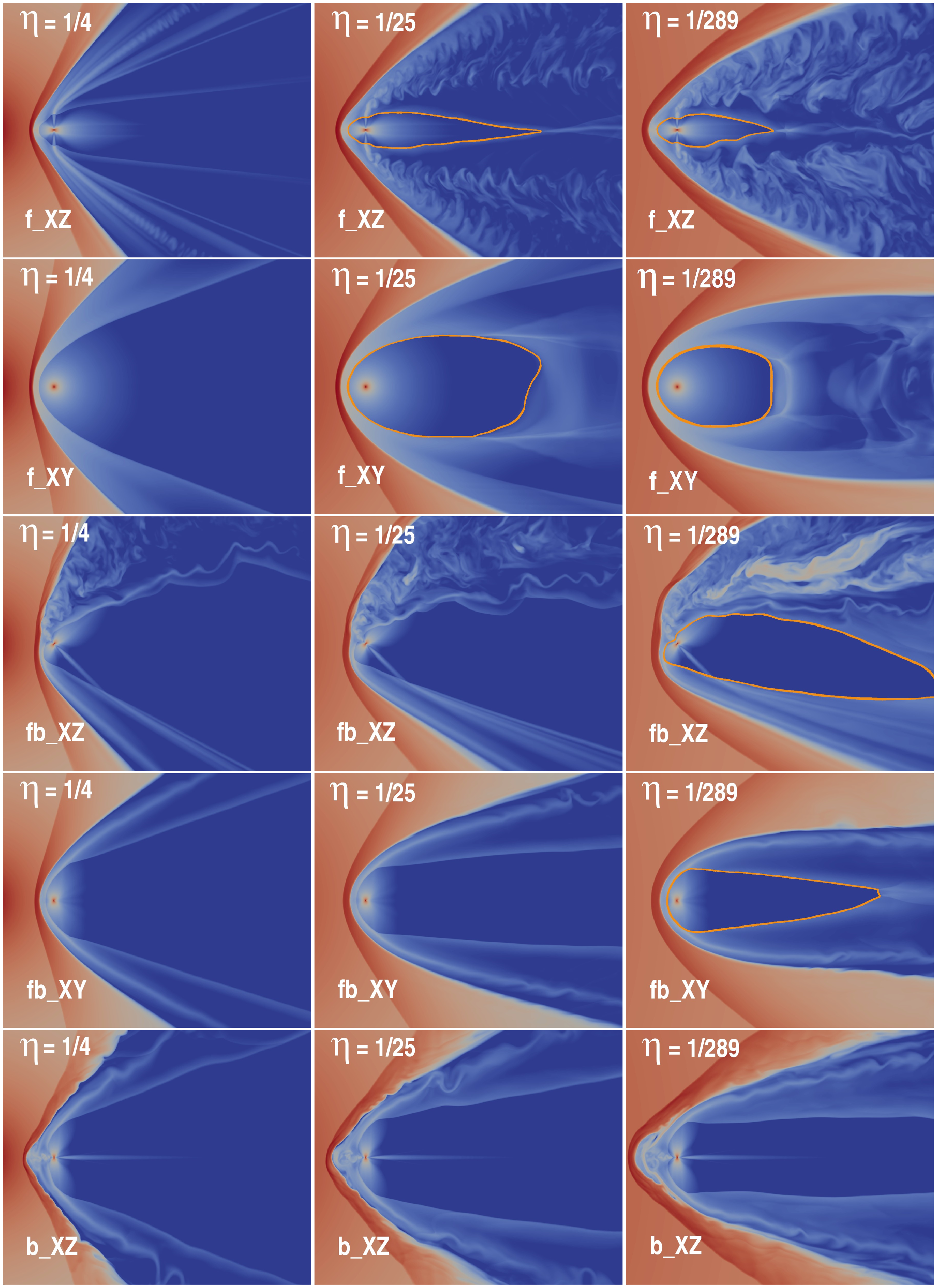
As we demonstrate in this paper, the open-closed dichotomy also depends on the orbital-dependent geometrical properties of the pulsar wind, for example, Fig. 3. The same system may evolve into different configurations depending on the orbital phase. On the Fig. 3 we indicated a position of the RS in pulsar wind by orange line.
Density (colour) for the models with η = 1/4 (left column), η = 1/25 (central column), and η = 1/289 (right column). At the first row ‘Frisbee’ XZ-plane and the second row XY-plane, the ‘Frisbee-Bullet’ XZ-plane and XY-plane on the third and fourth rows, respectively, and the ‘Bullet’ XZ-plane on the fifth row. The position of the reverse shock in pulsar wind is indicated by orange line.
In order to understand the complicated orbital-dependent behaviour of these systems, we performed a set of relativistic 3D magnetohydrodynamics (MHD) simulations of the interaction of the relativistic pulsar wind with the stellar wind. We rely on (and extend) two previous related investigations: hydrodynamic models of the wind–wind interaction in gamma-ray binaries (Bogovalov et al. Reference Bogovalov, Khangulyan, Koldoba, Ustyugova and Aharonian2008, Reference Bogovalov, Khangulyan, Koldoba, Ustyugova and Aharonian2012; Bosch-Ramon et al. Reference Bosch-Ramon, Barkov, Khangulyan and Perucho2012; Bosch-Ramon, Barkov, & Perucho Reference Bosch-Ramon, Barkov and Perucho2015; Valenti Bosch-Ramon et al. Reference Bosch-Ramon, Barkov, Mignone and Bordas2017; Barkov & Bosch-Ramon Reference Barkov and Bosch-Ramon2016, Reference Barkov and Bosch-Ramon2021; Lamberts et al. Reference Lamberts, Fromang, Dubus and Teyssier2013; Dubus et al. Reference Dubus, Lamberts and Fromang2015; Huber et al. Reference Huber, Kissmann and Reimer2021) and 3D relativistic MHD (RMHD) simulations of the pulsar wind–ISM interaction (Barkov et al. Reference Barkov, Lyutikov and Khangulyan2019a,b; Olmi & Bucciantini Reference Olmi and Bucciantini2019).
In the case of fluid simulations, Bosch-Ramon et al. (Reference Bosch-Ramon, Barkov, Khangulyan and Perucho2012, Reference Bosch-Ramon, Barkov and Perucho2015) found that the wind–wind interaction is subject to strongly non-linear processes already within the orbital scale that leads to the isotropisation of the interaction region and loss of coherence. Eventually the interacting region becomes an irregular isotropic flow formed by mixed stellar and pulsar winds. This mixed flow terminates with a shock on the external medium (interstellar medium (ISM)) or the interior of a supernova remnant (SNR).
Near the bow shock region, one can adopt the interaction of a magnetised pulsar wind with the ISM as an approximate model for the interaction of a pulsar and a stellar wind. Recently, two papers (Barkov et al. Reference Barkov, Lyutikov and Khangulyan2019a,b) have presented a study of the formation of PWN from a fast-moving pulsar. These works show that the geometry head of the bow shock and the pulsar wind tail can be significantly affected by the formation of the jet-like structures along pulsar spin axis. The CD in the pulsar wind tail can take the form of a cross (in ‘Frisbee’ case), instead of a cylindrical shape, as in the case of a spherically symmetric non-magnetised wind moving fast and interacting with the ISM. This cross shape of the CD is the result of the asymmetry of the pulsar wind, which is dominated by the equatorial flow and the jet-like structures in the polar directions.
The paper has the following structure: (1) Introduction; (2) Details of the simulation set-up (stellar wind and pulsar wind set-up); (3) Simulation results with a detailed comparison with 2D relativistic hydrodynamics (RHD) and 2D RMHDFootnote a and a detailed discussion of the flow in general; and (4) Discussion and conclusions.
2. Details of the simulations’ set-up
The initial set-up of our simulation for the magnetised pulsar wind is similar to our previous work for the interaction of the ISM with the relativistic wind of a fast-moving pulsar (Barkov et al. Reference Barkov, Lyutikov and Khangulyan2019a, see also Porth, Komissarov, & Keppens Reference Porth, Komissarov and Keppens2014). As a first step, we focus on the bow shock structure and study the formation of tailward Mach discs, neglecting the orbital motion of the pulsar.
The simulations were performed using a three-dimensional (3D) geometry in Cartesian coordinates using the PLUTO codeFootnote
b
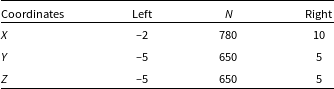
(Mignone et al. Reference Mignone, Bodo, Massaglia, Matsakos, Tesileanu, Zanni and Ferrari2007). Spatial linear interpolation, a second-order Runge–Kutta approximation in time, and an Harten-Lax-van Leer (HLL) Riemann solver were used (Harten Reference Harten1983). PLUTO is a modular Godunov-type code entirely written in C and intended mainly for astrophysical applications and high Mach number flows in multiple spatial dimensions. The simulations were performed on CFCA XC50 cluster of National Astronomical Observatory of Japan (NAOJ). The flow has been approximated as an ideal, relativistic adiabatic gas, one particle species, and polytropic index of 4/3. The size of the domain is
 $x \in \left[ {-2,\;10} \right],$
 $y$
and
 $z \in \left[ {-5,{\rm{\;}}5} \right]$
. We have uniform resolution in the entire computational domain with total number of cells
 ${N_X}$
= 780, and
 ${N_Y}$
=
 ${N_Z}$
= 650; see details in Table 1.
2.1 Stellar wind set-up
The stellar wind is simulated as an already formed, full-speed, supersonic radial flow centred in the star location carrying toroidal magnetic field. To make the simulation computationally lighter, we use a non-uniform resolution in the computational domain. All these assumptions allow us to use a much larger resolution at the region encompassing the pulsar and its bow shock, as well as a large linear size of the computational domain.
In our model the normal star has place outside the computational domain, because of supersonic inflow on the left X edge (X = –2) we can inject such the stellar wind. For models r3 we set the normal star position at the point (-3,0,0), for r6 at the point (-6,0,0), and r18 at the point (-18,0,0).
We start our simulation from a non-equilibrium configuration and evolve it up to the time at which quasi-stationary solution is reached. To reduce computational expenses, we set the stellar wind speed as
 ${v_{{\rm{wind}}}} = 0.1c$
and Mach number M = 85. The density of the stellar wind was adopted so that in the case of non-magnetised spherical pulsar wind, the bow shock is formed at the position near (–1, 0, 0). The wind speed value is not realistic, but it is not significantly affecting the volume inside the CD (Barkov, Lyutikov, & Khangulyan Reference Barkov, Lyutikov and Khangulyan2020). The stellar wind have weak magnetisation
 ${\sigma _{{\rm{wind}}}}$
= 0.01, which is formed by toroidal/axisymmetric (Y-axis) magnetic field in the plane-XZ.
This set-up has several free parameters which we vary in our simulations: (i) changing the pulsar distance to the normal star while keeping the distance to the bow shock constant (in dimensional less units, actual distance from pulsar to standing point in the RS is function of
 $\eta $
) allows us to inspect how sensitivity is the numerical solution to variations of the non-dimensional momentum-rate ratio, the pulsar wind magnetisation, and the orientation of pulsar rotation axis (i.e. the magnetic field toroidal geometry) relative to the direction to the normal star; (ii) we study different spin orientations of the pulsar with respect to the wind velocity (as the pulsar moves along the orbit the orientation of the pulsar spin change with respect to the wind direction, except in the case when pulsar spin axis is perpendicular to the orbital plane); and (iii) we include the rotation of the pulsar spin axis along the orbit, which mimics the effect of orbital motion.
Parameters of the computational grid.
2.2 Pulsar wind set-up
The pulsar emits the unshocked magnetised pulsar wind with a toroidal magnetic field, which changes its polarity in the northern and southern hemispheres.
In our work we use the prescription of pulsar wind described in the paper (Porth et al. Reference Porth, Komissarov and Keppens2014), see details in the Appendix A. The pulsar with radius 0.15 is placed at the point (0,0,0). The pulsar wind was injected with the initial Lorentz factor
 $\Gamma $
= 1.7 and Mach number 25. For all models, we adopt the same magnetisation parameter
 ${\sigma _0}$
= 1Footnote
c
and angle between the magnetic and rotation axis
 $\alpha = \pi /4$
. The thrust ratio of the pulsar and stellar wind was chosen to form a bow shock at the distance of 1 for the spherical pulsar wind. Parameters for the models are presented in the Table 2.
We choose three cases of pulsar orientation ‘Frisbee’, ‘Bullet’, and intermediate one ‘Frisbee-Bullet’ (Barkov et al. Reference Barkov, Lyutikov and Khangulyan2019a). In the case of the ‘Frisbee’, the pulsar rotation axis is parallel to the axis Z (
 $\zeta = 0$
), in the case of the ‘Bullet’ the pulsar rotation axis is parallel to the axis X (
 $\zeta = \pi /2$
), the intermediate case was formed by clockwise turn of the ‘Frisbee’ configuration around the Y-axis at angle
 $\zeta = \pi /4$
. Such change of configurations is natural if the pulsar rotation axis lays in the orbital plane.
Parameters of the models. (1) Name of the model; (2) angle between direction to the star and pulsar spin axis; (3) stellar and pulsar wind thrust ratio; (4) distance to the normal star in the bow shock radius units; (5) angle between magnetic and rotation axis of pulsar.
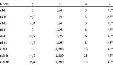
We performed calculations for nine models, as we vary the η parameter and pulsar orientation in respect to direction to the normal component, Table 2. These static cases can be interpreted as evolution of the spin axis in the binary system if the pulsar spin lies in the orbital plane. Thus, neglecting the influence of the magnetic field in the stellar wind (which was chosen small and dynamically not important) we can also interpret our results as different individual binary systems with various orientation of spin axis in respect to orbital plane. It can be systems with three sequences: (1) if the pulsar spin axis is normal to the orbital plane, we have ‘Frisbee’ all the time; (2) if the pulsar spin axis angled on
 ${45^{\rm{o}}}$
to the orbital plane, we have transition ‘Frisbee’ − ‘Frisbee-Bullet’ − ‘Frisbee’ every half of the orbit; and (3) if the pulsar spin axis lay in the orbital plane, we have ‘Cartwheel’ − ‘Frisbee-Bullet’ − ‘Bullet’ − ‘Frisbee-Bullet’ − ‘Cartwheel’ every half of the orbit.
3. Results
3.1 ‘Bird’s-eye’ view
In Fig. 3, we demonstrate ‘bird’s-eye’ view of different configurations. We explore various thrust ratios (we consider cases
 $\eta \le 1{\rm{\;}}$
so that the resulting shock structure wraps around the pulsar) and effects of different internal geometries. While for not very small thrust ratio of
 $\eta = 1/4$
(left column) the differences between different geometries are mild, for very small thrust ratios of
 $\eta = 1/25\,{\rm{\;}}289$
we find qualitatively different behaviour for different orientations and different cuts.
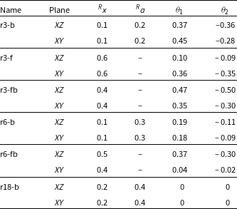
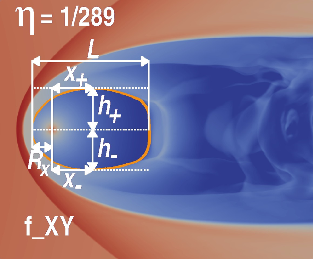
There are two different shock wave structures that we obtained: opened-in-the-back and closed, qualitatively described in Fig. 2; results of simulations are in Figs. 4–5. Opened configurations have two branches laying along
 $x$
-axis, which don’t intersect each other. The upper situation in Fig. 4 may be only in ‘Frisbee-Bullet’ orientation, and the lower situation may be in ‘Frisbee’ and ‘Bullet’ orientation. Otherwise, in closed configuration, two branches have the intersection point.
Sketches of two different configurations with open free wind zone. The upper case may be only in ‘Bullet’ orientation, and the lower case may be in ‘Frisbee’ or ‘Frisbee-Bullet’ orientation. The measured parameters for the models are presented in the Table 3.
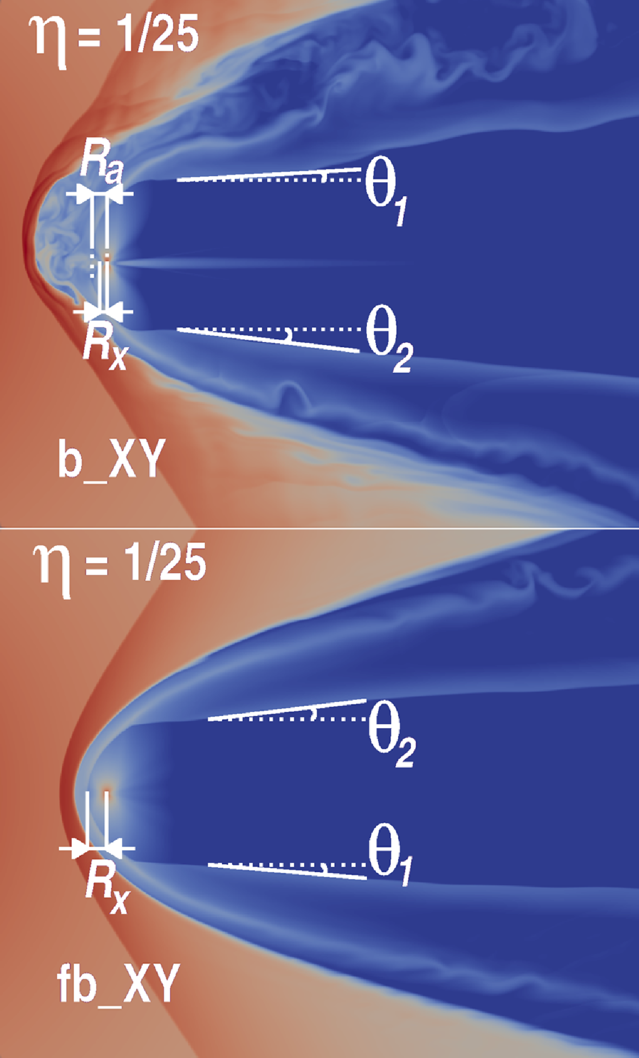
In Figs. 4 and 5, the cross indicates the location of the neutron star. The distance between the neutron star and the intersection point of the shock wave ‘head’ and
 $x$
-axis is denoted by
 ${R_x}$
. If the shock wave head has the apex point that don’t laying at the
 $x$
-axis (see upper sketch in Fig. 4), the corresponding distance along x-axis is denoted as
 ${R_a}$
. Also, in the case of open areas, the values of the angles between the branches and
 $x$
-axis
 ${\theta _1}$
and
 ${\theta _2}$
were calculated. The clockwise is positive direction, and the counterclockwise is negative. In the opposite situation of closed zone, the following parameters are calculated: the length of the zone from apex point to the end of the tail L, the locations of the maximum points in perpendicular directions to the
 $x$
-axis from the location of the neutron star (
 ${x_ + }$
and
 ${x_ - }$
) and from the
 $x$
-axis (
 ${h_ + }$
and
 ${h_ - }$
). The corresponding values of the parameters are presented in Tables 3 and 4.
Parameters of the shock waves – opened configuration.
Parameters of the shock waves – closed configuration.
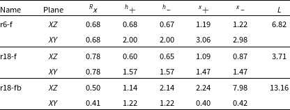
Sketch with close wind zone, which may be in situations with ‘Frisbee’ and ‘Frisbee-Bullet’ orientations. The measured parameters for the models are presented in the Table 4.
Dependence of angles
 ${{\rm{\theta }}_1}$
(upper) and
 ${{\rm{\theta }}_2}$
(lower) on the eta parameter
 $\eta $
. The ‘Frisbee’, ‘Bullet’ and ‘Frisbee-Bullet’ orientations were marked by ‘squares’, ‘triangles’ and ‘stars’ correspondingly. The measured parameters for the models are presented in the Table 3. The black thick solid line denotes the result obtained in the work (Bogovalov et al. Reference Bogovalov, Khangulyan, Koldoba, Ustyugova and Aharonian2008). The orange and purple dots denote the opening angles for magnetisation
 $\sigma $
0.8 and 0 correspondingly obtained in the work (Bogovalov et al. Reference Bogovalov, Khangulyan, Koldoba, Ustyugova and Aharonian2019).
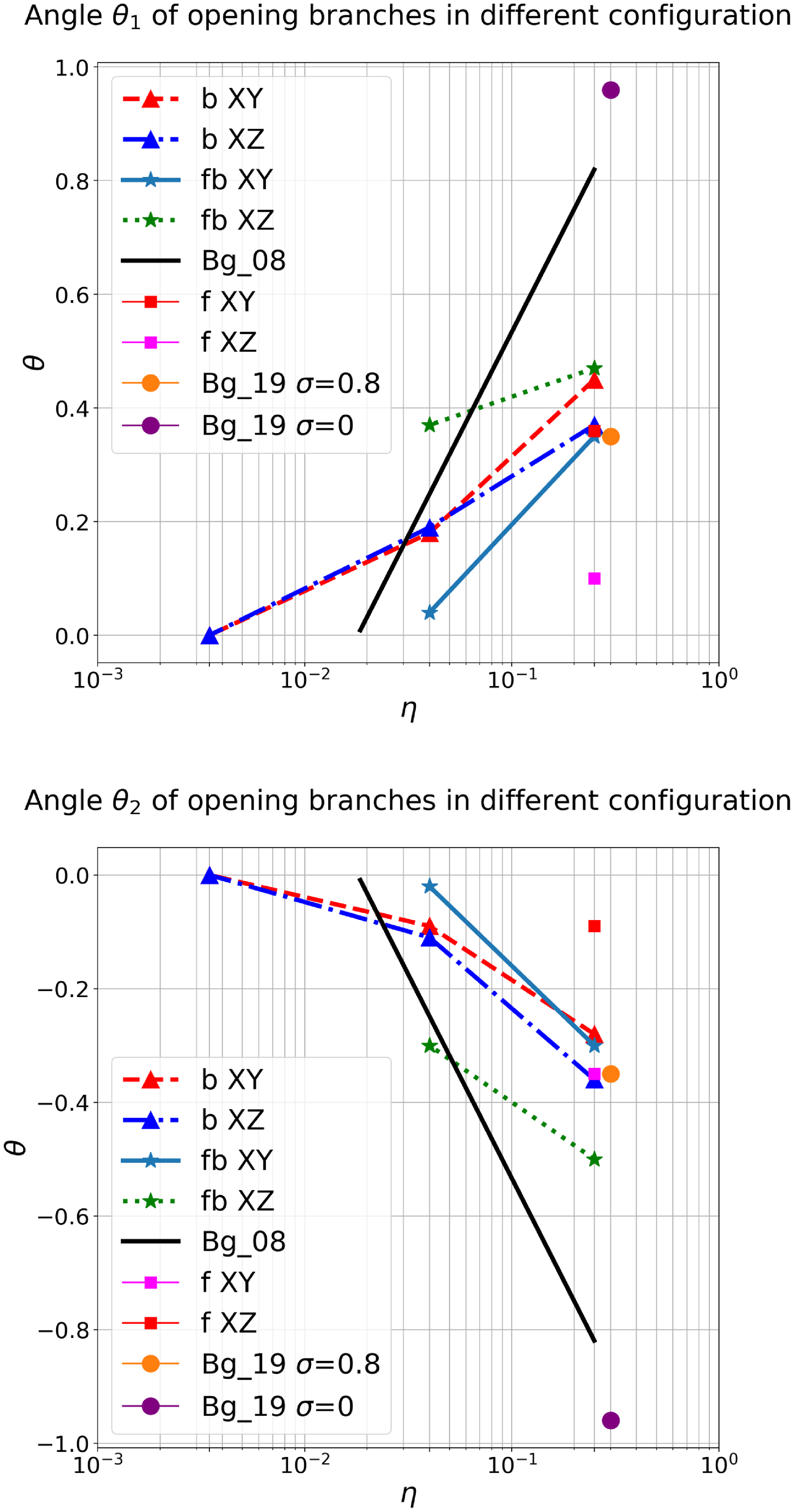
In Figs. 6–7, we presented the dependence of the geometrical properties on the parameters of the simulations. In these figures, ‘squares’, ‘triangles’, and ‘stars’ denote ‘Frisbee’, ‘Bullet’, and ‘Frisbee-Bullet’ orientation correspondingly. The
 $\eta $
parameter was chosen as the parameter of the
 $x$
-axis, which has the connection with distance from neutron star to normal star:
 \begin{align}\frac{r}{a} = \frac{{\sqrt \eta }}{{1 + \sqrt \eta }},\end{align}
Dependence of length of tail L_tail on the eta parameter η. The ‘Frisbee’ and ‘Frisbee-bullet’ orientations were marked by ‘squares’ and ‘stars’ correspondingly. The measured parameters for the models are presented in the Table 4. The black thick solid line denotes the result obtained in the work (Bogovalov et al. Reference Bogovalov, Khangulyan, Koldoba, Ustyugova and Aharonian2008).
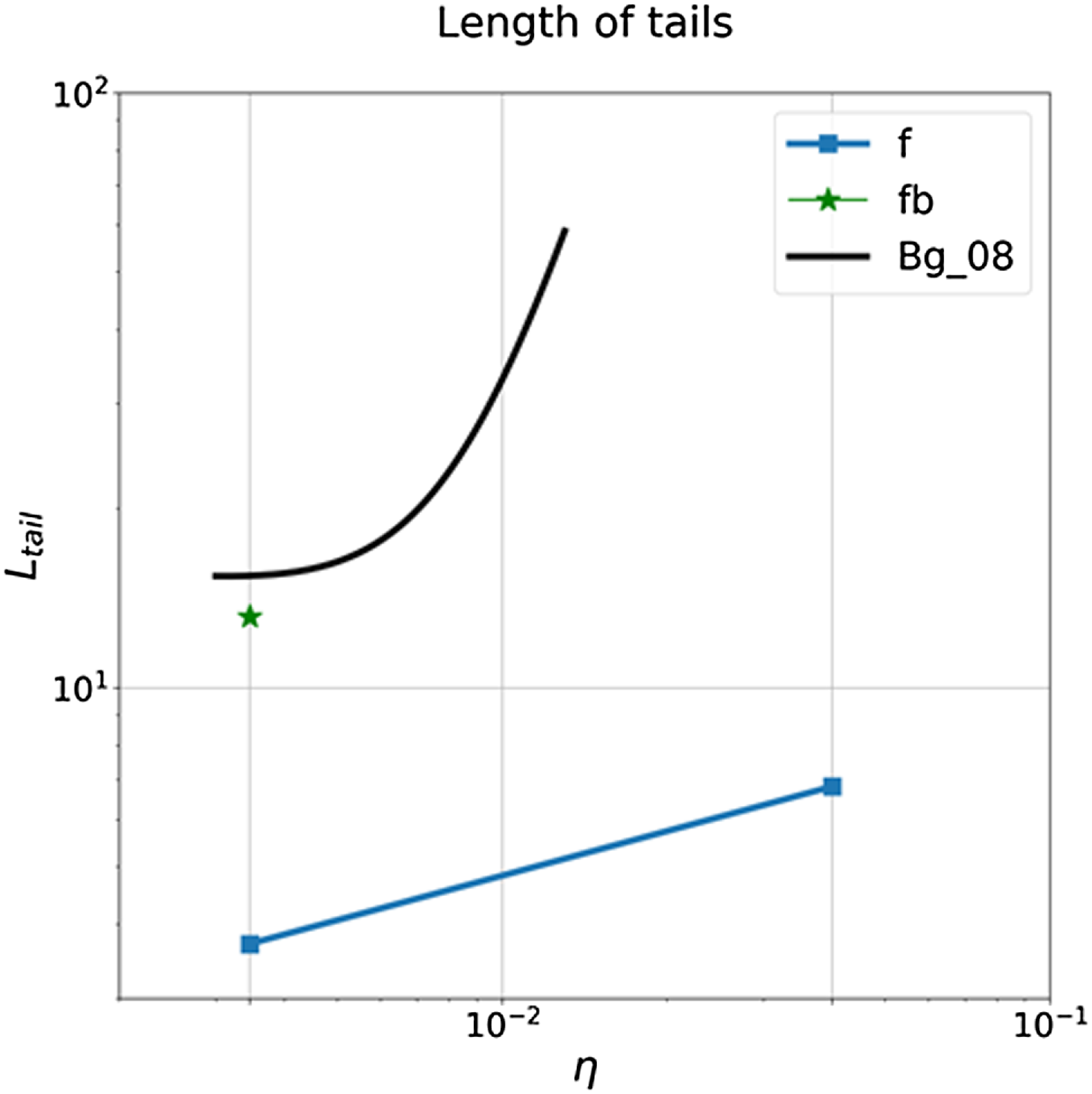
One can see that wind zone expands with increasing of
 $\eta $
parameter. This result has the similarities with the paper Bogovalov et al. (Reference Bogovalov, Khangulyan, Koldoba, Ustyugova and Aharonian2008). In Fig. 6, the black thick solid line means the result obtained by Bogovalov et al. (Reference Bogovalov, Khangulyan, Koldoba, Ustyugova and Aharonian2008). But this dependence on the eta parameter has a gradient that is greater than when taking into account the magnetic field. On the other hand, not taking into account magnetic field by Bogovalov et al. (Reference Bogovalov, Khangulyan, Koldoba, Ustyugova and Aharonian2008) leads to critical value of the
 $\eta $
parameter, which means that there are only opened configurations for greater values η. Fig. 7 shows that closed configuration takes place when magnetic field has Frisbee or Frisbee–Bullet orientation, and wind zone can take smaller values of tail lengths compared to the result without taking into account the magnetic field.
In other words, for pulsar with the spin axis in the orbital plane, the length of the free wind zone can change from 1/4 orbital separation till
 $x \approx 3{v_w}/2{\rm{\Omega }}{\eta ^{1/2}}~2T_{{\rm{orb}},\;\;6}^{1/3}{\eta ^{1/2\;}}$
(Barkov & Bosch-Ramon Reference Barkov and Bosch-Ramon2021). So photon–photon absorption can vary in one order of magnitude and lead to strong variation of gamma-ray signal during orbital period (see as example Khangulyan, Aharonian, & Bosch-Ramon Reference Khangulyan, Aharonian and Bosch-Ramon2008; Zabalza et al. Reference Zabalza, Bosch-Ramon, Aharonian and Khangulyan2013).
3.2 Dynamics of the magnetised wind
Next, we discuss the internal magnetic field structure of the flow. In Figs. 8−10, we show a complex plot of pressure (by colour) which is projected on the CD surface and streamlines showing magnetic field strength by its thickness and colour.
The pressure (colour) and magnetic field lines (streamlines) for models with η = 1/4 r3-f (top panel), r3-fb (middle panel) and r3-b (bottom panel). We extrude the data at the contact discontinuity based on the jump of density and put half-transparent surface of pressure by colour. The thickness of the streamlines indicates the strength of the magnetic field. The quantities B_0 and p_0 are means the units of magnetic field and pressure consequently (B_0 is equal to 52 G and p_0 is equal to 137 bar).
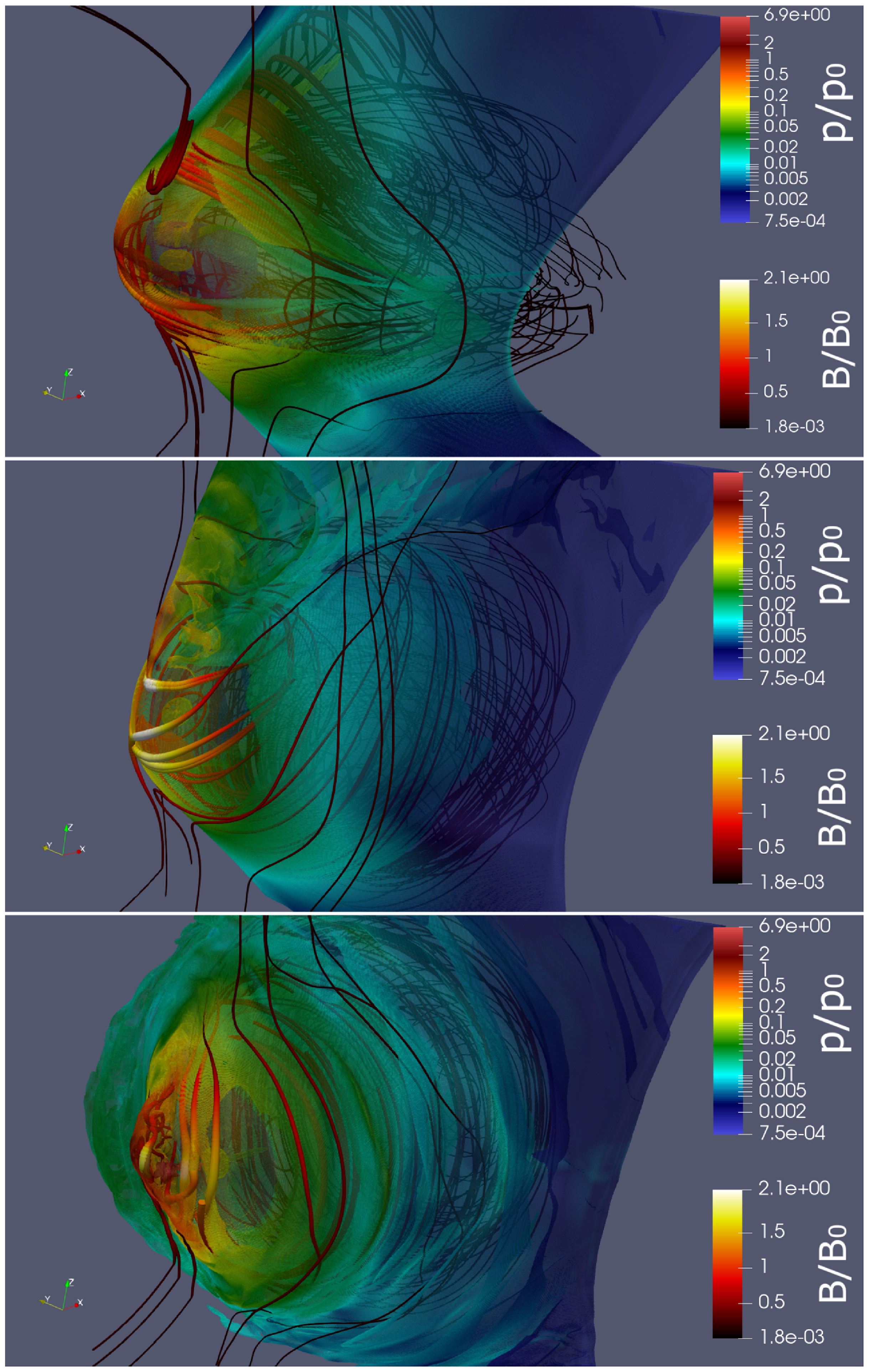
Same as Fig. 8 for models with η = 1/25 r6-f (top panel), r6-fb (middle panel) and r6-b (bottom panel). We extrude the data at the contact discontinuity based on the jump of density and put half-transparent surface of pressure by colour. The thickness of the streamlines indicates the strength of the magnetic field. The quantities B_0 and p_0 are means the units of magnetic field and pressure consequently (_0 is equal to 42 G and p_0 is equal to 88 bar).
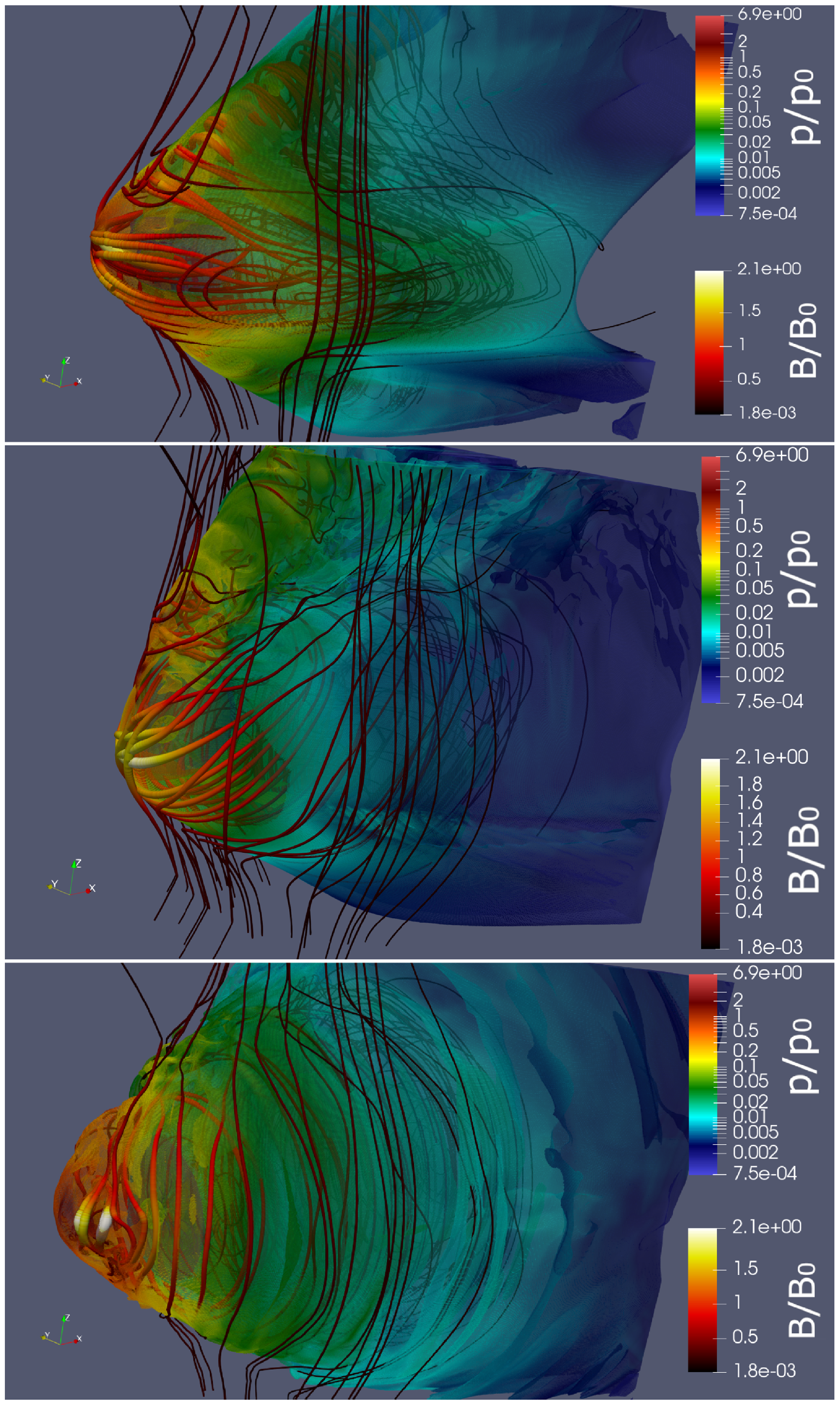
Same as Fig. 8 for models with η = 1/289 r18-f (top panel), r18-fb (middle panel) and r18-b (bottom panel). We extrude the data at the contact discontinuity based on the jump of density and put half-transparent surface of pressure by colour. The thickness of the streamlines indicates the strength of the magnetic field. The quantities B_0 and p_0 are means the units of magnetic field and pressure consequently (B_0 is equal to 37 G and p_0 is equal to 68 bar).
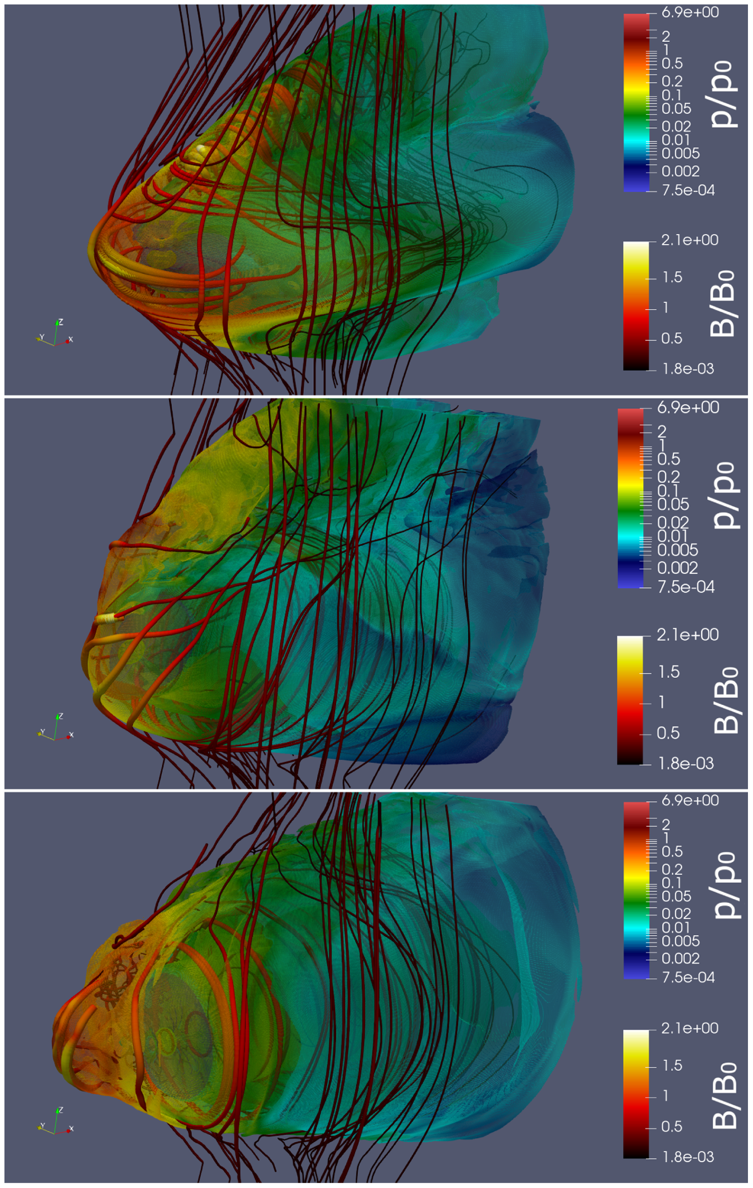
We find that the shape of the CD changes from almost conical one (‘Bullet’ cases), transformed to flattened structure for the ‘Frisbee-Bullet’ cases, and cross for ‘Frisbee/Cartwheel’. The jet in the ‘Bullet’ configurations pushed bow shock closer to the normal star and magnetic field near CD head of the jet is significantly increased compare to ‘Frisbee-Bullet’ and ‘Frisbee/Cartwheel’ cases.
In Figs. 11–13, we present density and streamlines distribution, and colour indicates velocity magnitude for different winds thrust ration
 $\eta = {\raise0.7ex\hbox{$1$} \!\mathord{\left/ {\vphantom {1 4}}\right.}\!\lower0.7ex\hbox{$4$}}$
,
 $\eta $
= 1/25, and
 $\eta $
= 1/289, respectively. On all plots, we see standard structure of the flow which consist of free stellar wind and pulsar wind separated by shocked pulsar wind and stellar wind. The magnetic field significantly affects the flow from the pulsar. In an equatorial plane wind is stronger (see Equation (A1)) but in the polar direction hoop stress climate flow in the jet-like structures.
The density (colour) and velocity distribution (streamlines) for the models with η = 1/4 r3-f (top panel), r3-fb (middle panel) and r3-b (bottom panel). The quantities ρ_0 and c means the units of density and speed consequently (ρ_0 is equal to 6.33 × 10⁻¹⁸gr/cm3 and c is the speed of light).
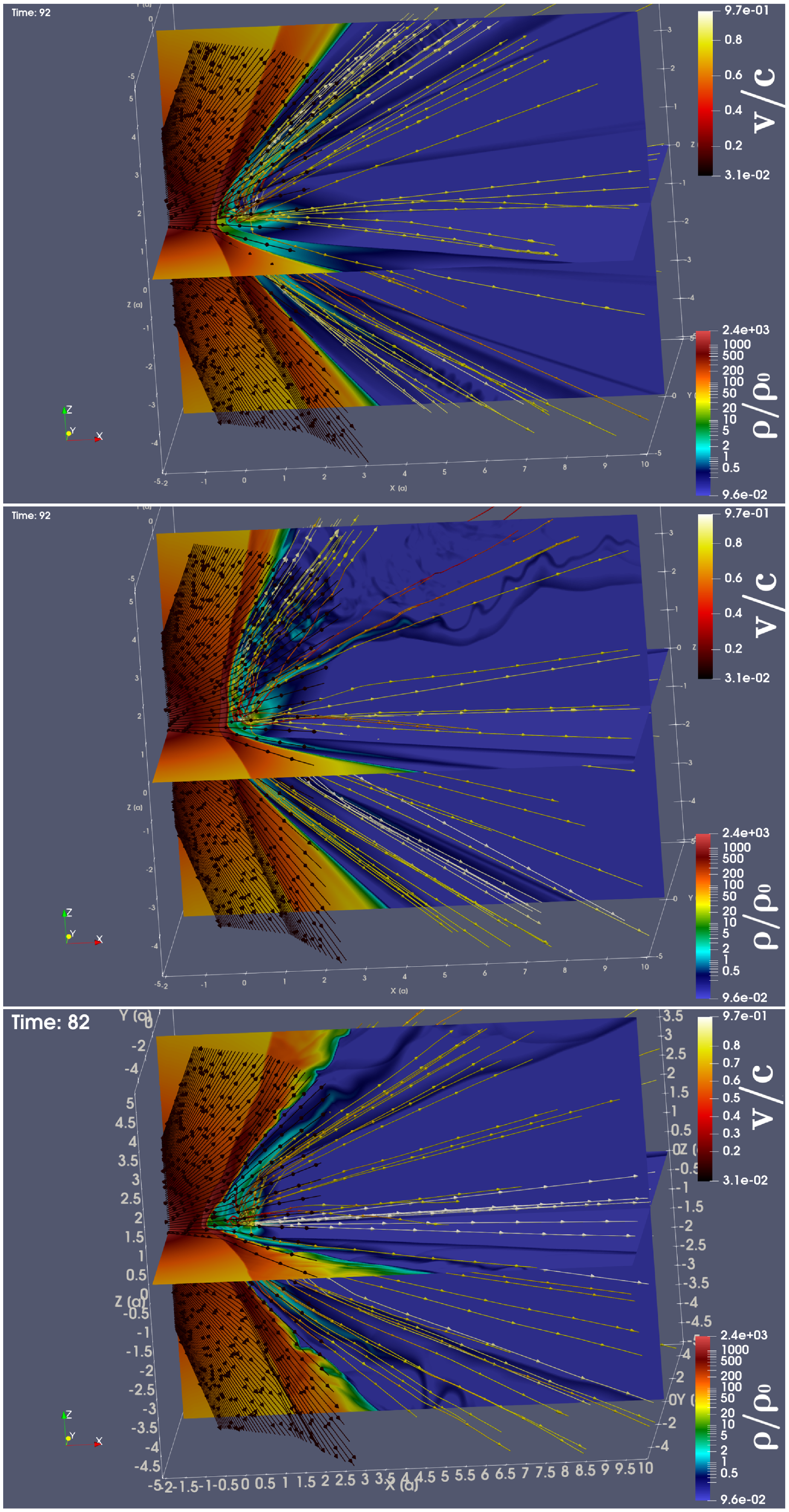
The density (colour) and velocity distribution (streamlines) for the models with η = 1/25 r6-f (top panel), r6-fb (middle panel) and r6-b (bottom panel). The quantities ρ_0 and c means the units of density and speed consequently (ρ_0 is equal to 4.05×10⁻¹⁸ gr/cm3 and c is the speed of light).
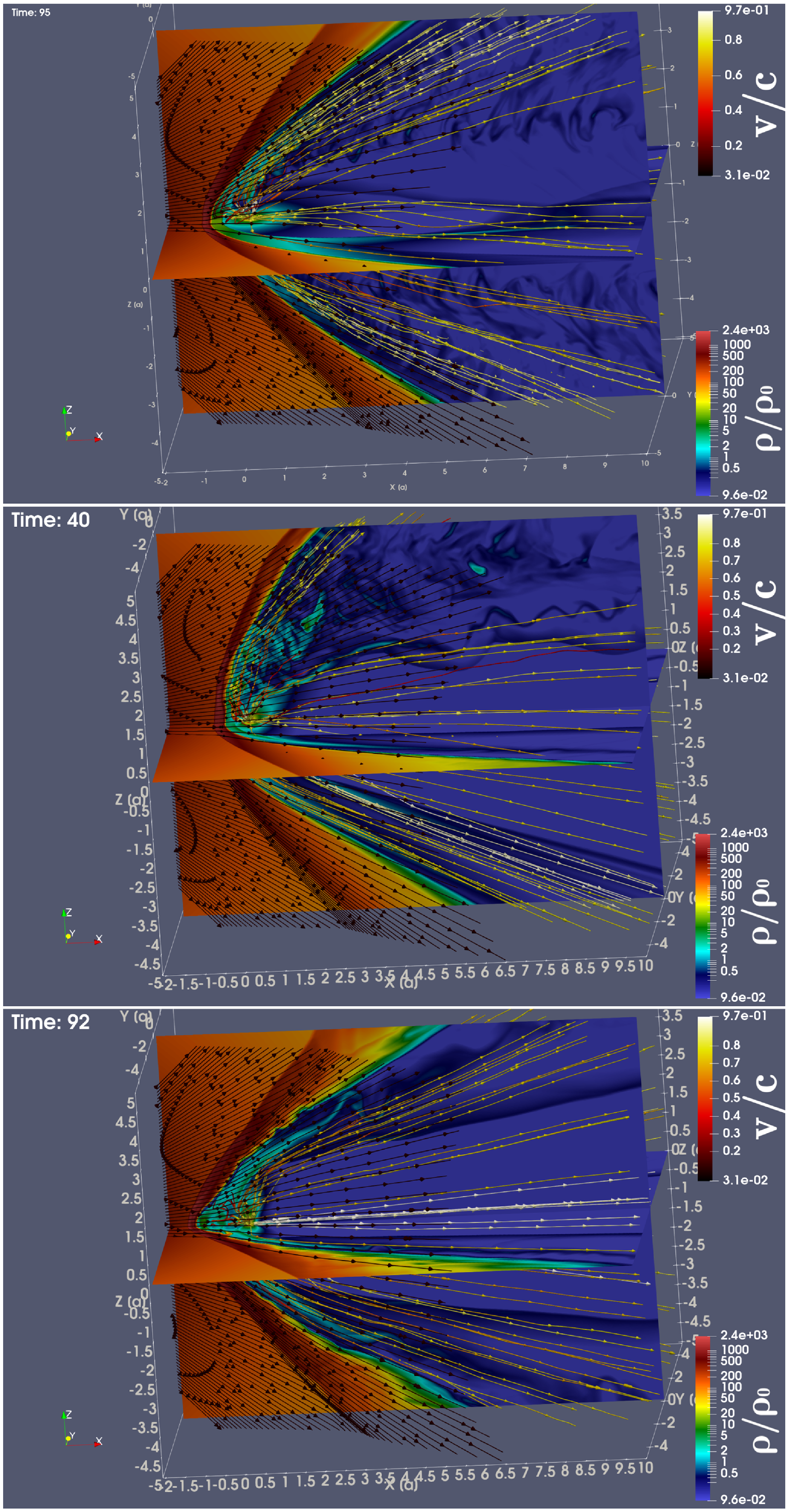
The density (colour) and velocity distribution (streamlines) for the models with η = 1/289 r18-f (top panel), r18-fb (middle panel) and r18-b (bottom panel). The quantities ρ_0 and c means the units of density and speed consequently (ρ_0 is equal to 3.15×10⁻¹⁸gr/cm3 and c is the speed of light)
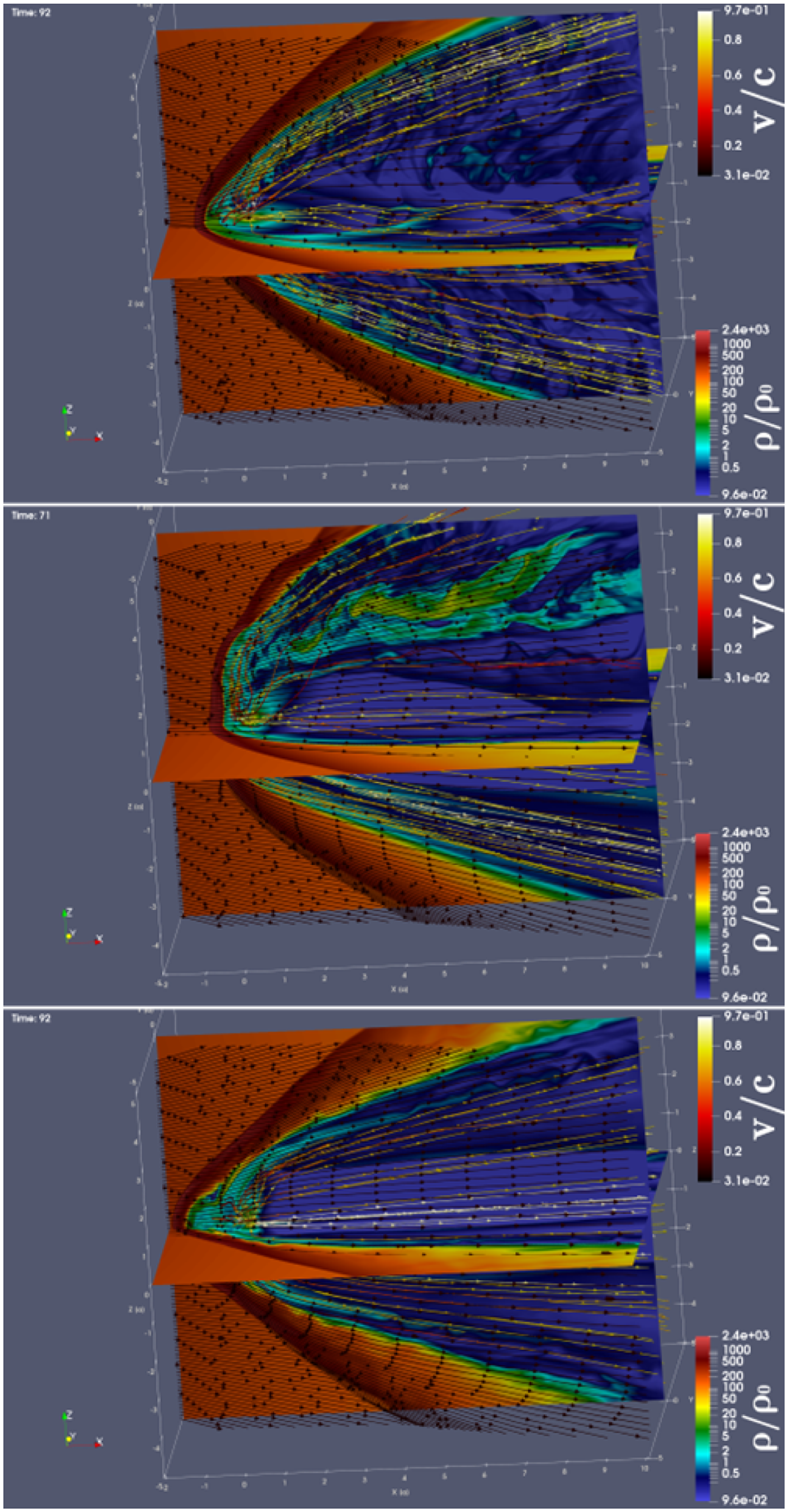
The density plots indicate clearly the CD. The angle of the CD is dependent on the η parameter and less sensitive to the pulsar orientation. The position of the pulsar wind shock, much more sensitive to the pulsar orientation. The higher η parameter leads to smoother (more laminar) flow for all orientations, smaller η leads to more turbulent flow. The ‘Bullet’ configuration forms turbulent motion near CD, but near pulsar wind shock the flow is smooth. The ‘Cartwheel’ or ‘Frisbee-Bullet’ cases show strong turbulence in polar regions, especially if it is inclined onto normal star.
In Fig. 3, we presented the density cuts in different planes. Here, we clearly see shocks in the stellar wind and in the pulsar wind. The orientation of the pulsar significantly affects the RS geometry. The results in general are similar to results obtained in the works (Barkov et al. Reference Barkov, Lyutikov and Khangulyan2019a,b). For higher values of
 $\eta $
parameters, the flow become more expanding, but the general topology is preserved.
4. Radiation processes
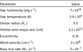
We calculated the non-thermal emission of the pulsar in high-mass binary system, as a prototype, we chose LS 5039. The properties of the binary system used are shown in Table 5 (Casares et al. Reference Casares, Ribo, Ribas, Paredes, Marti and Herrero2005). Thus, using the formula 1 one can find the spin-down luminosity of a neutron star (see Table 6). The bolometric luminosity of the system is dominated by optical emission of the normal massive star. On the other hand, non-thermal radiation processes are controlled by the SYN and IC (see for details Khangulyan et al. Reference Khangulyan, Aharonian and Bosch-Ramon2008), and
 $\gamma - \gamma $
absorption has a significant effect on hard radiation and has to be taken into account as well. Our emissivity model is similar to the described in the (Bosch-Ramon & Khangulyan Reference Bosch-Ramon and Khangulyan2009; Khangulyan, Aharonian, & Kelner Reference Khangulyan, Aharonian and Kelner2014), details are presented in the Appendix B.
To evaluate the gamma–gamma absorption process, optical thickness
 $\tau = \smallint n\sigma d$
was calculated assuming maximum cross section for two-photon pair production
 $\sigma $
(
 ${\sigma _T}$
/5) was selected. Optical thickness
 ${\tau _0}$
was calculated for one point located at a unit distance from a massive star, then the remaining values along one straight line were calculated using the scaling property of the optical thickness (see formula (12) Khangulyan et al. Reference Khangulyan, Aharonian and Bosch-Ramon2008) as:
 \begin{align}\tau = {\tau _0}\frac{d}{l},\end{align}
where
 ${\tau _0}$
is evaluated optical thickness on the distance
 $d = 1$
from star,
 $l$
is the distance for which we evaluate thickness
 $\tau $
.
The emissivity for the IC and SYN processes was calculated using the formula
 $I^{\prime}_{rad} \propto \smallint \left( {{u_{cell}}/{t_{rad}}} \right)d\ell $
, where
 $\ell $
is the length element along the line of sight (see Barkov & Bosch-Ramon Reference Barkov and Bosch-Ramon2018). We take into account the power-low distribution of electrons with spectra
 $n = A{ \in ^{ - \alpha }}$
there an
 $\alpha $
= 2. The resulting value describes the emissivity of the system in its own frame of reference. The Doppler factor
 $\delta $
(see Appendix B) is used to convert the emissivity from the co-moving reference frame
 $I_\nu ^{\rm{'}}$
to a laboratory reference frame
 ${I_\nu }$
. Thus, the emissivity for
 $\alpha $
= 2 is converted by the formula.
 \begin{align}{I_\nu } = {\delta ^{2.5}}I_\nu ^{\rm{'}},\end{align}
In particular, in the case of the IC process, gamma absorption of gamma radiation was taken into account by multiplying by an additional factor:
 \begin{align}{I_{IC}}{\rm{\;}} = {\rm{\;}}{I_\nu }{\rm{exp}}\left( {-\tau } \right),\end{align}
where
 $\tau $
is the optical thickness (see formula (3)).
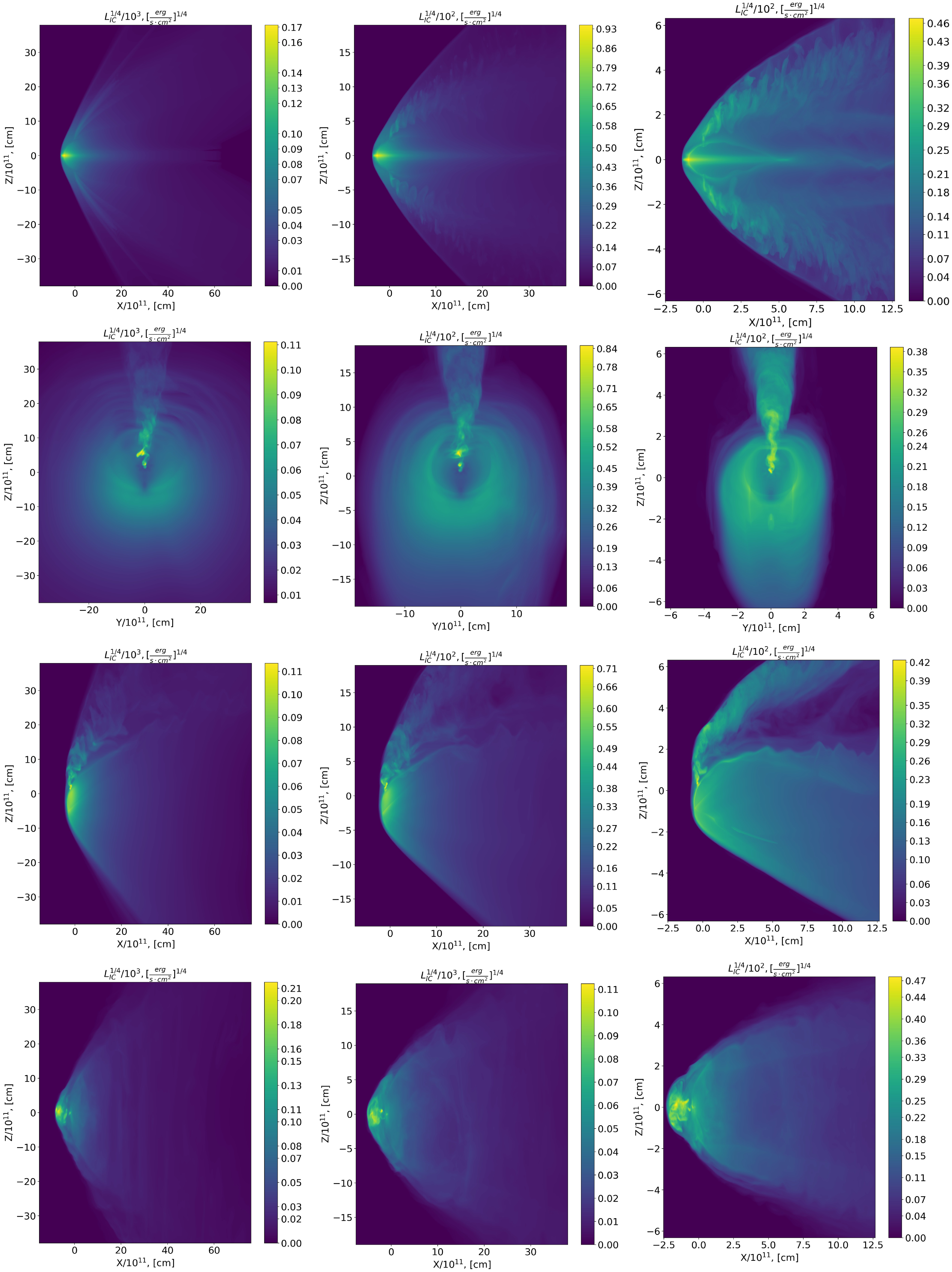
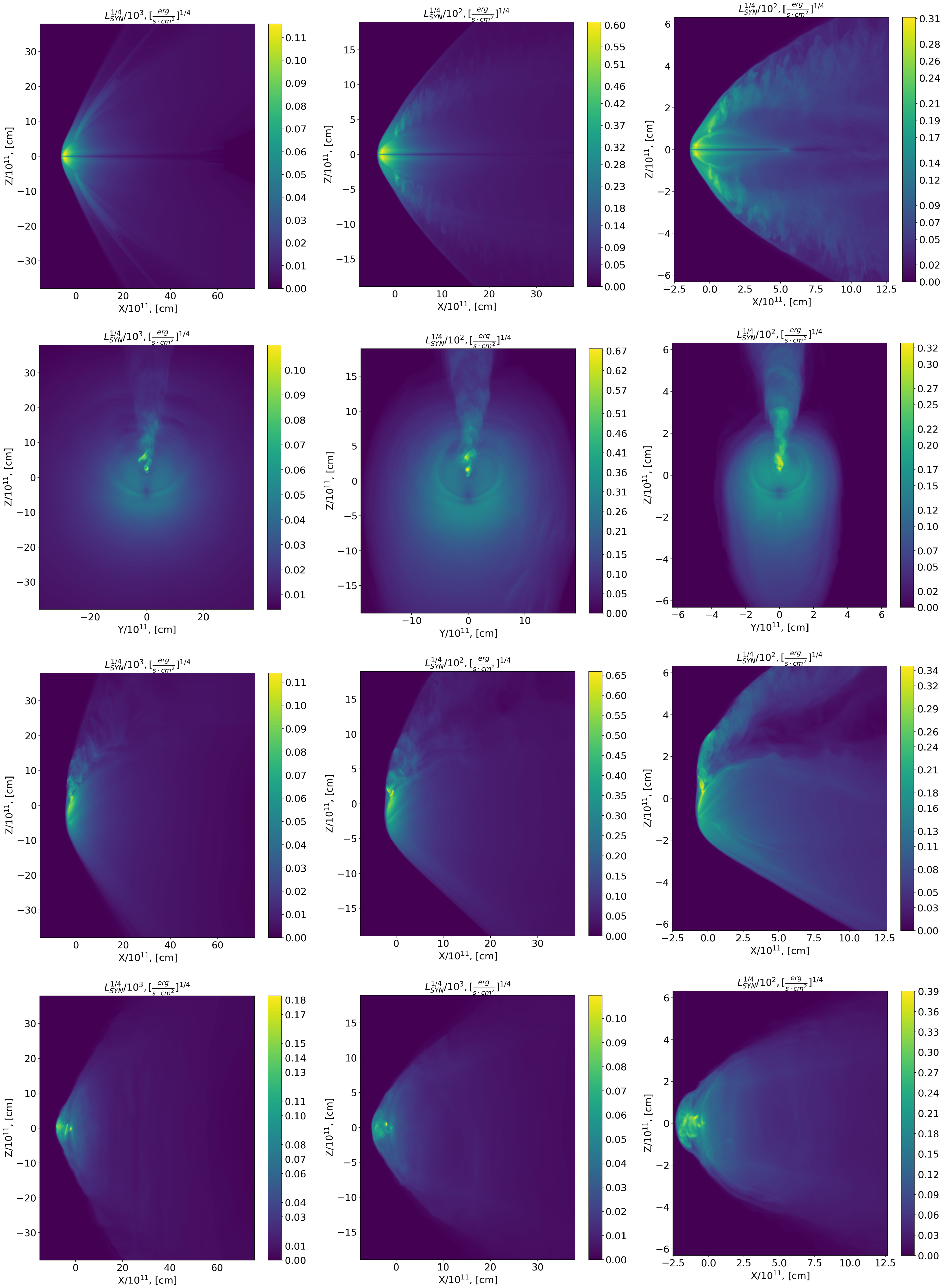
We calculated emissivity maps which describe the system emission along the X, Y, Z axes (lines of sight, see Figs. 14 and 15). The flow from the neutron star which form jets and the front bow shock are the brightest details. Next one is the pulsar shocked wind at larger distance from the pulsar which form quite bright background. We should note, the bright element of the flow is the back shock and pulsar equatorial region, which in total can give luminosity values comparable to the luminosity of individual parts of the front shock.
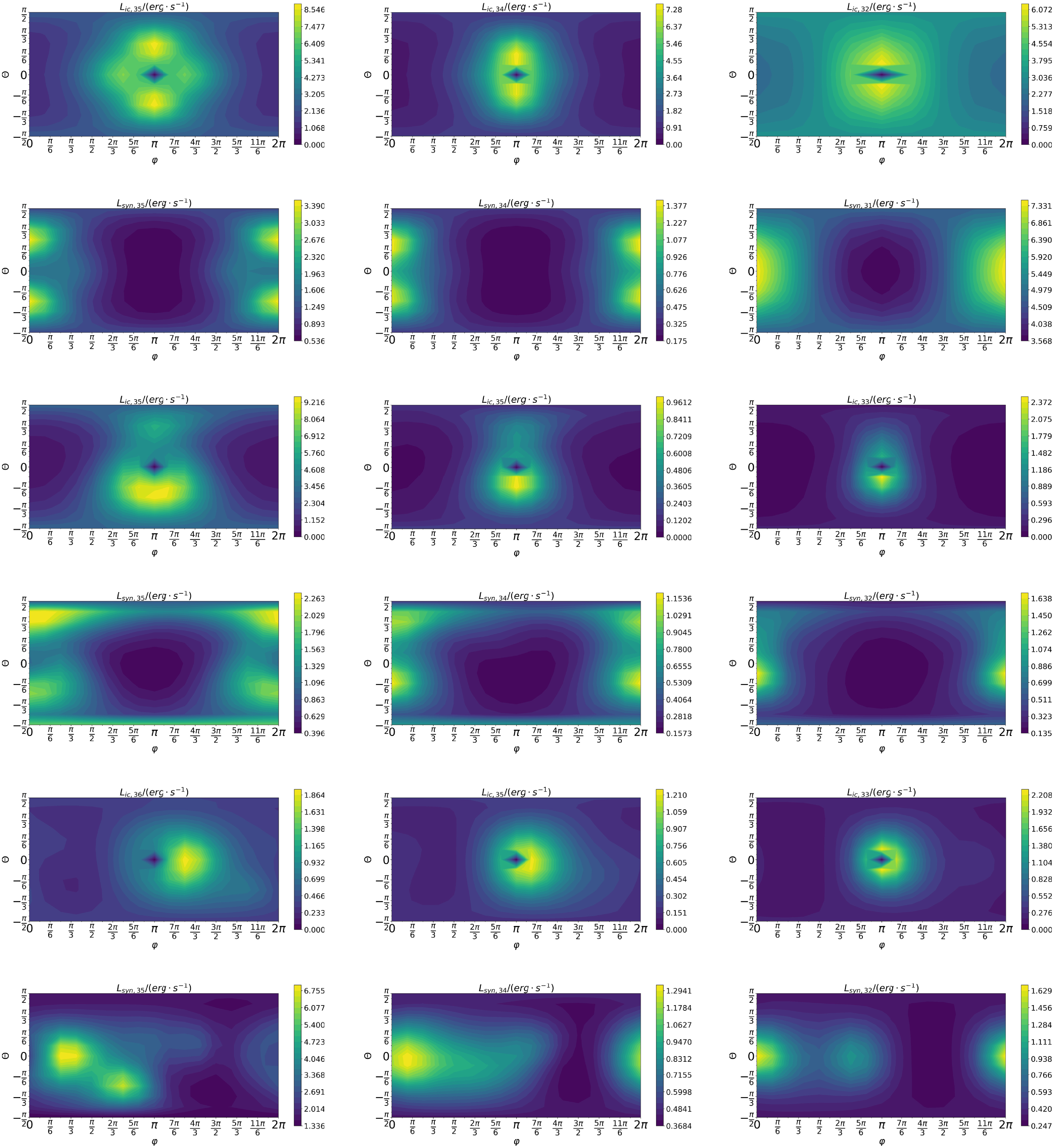
The luminosity maps depending on the polar (
 $\theta $
) and azimuthal (
 $\varphi $
) angles are presented on (Fig. 16), for sake of simplicity here and below we set eccentricity
 $ \in = 0$
. Further, other possible directions of the lines of sight to this system were considered, and the obtained emissivity was summed up over the entire surface, that is, the luminosity of the system for this line of sight was obtained. For visualisation of the results obtained, lines of luminosity levels were plotted according to the angles of view (Fig. 16). The polar angle of
 $\theta $
is calculated from the orbital plane and takes values from
 $\pi /2$
(along the selected Z-axis) to
 $-\pi /2$
(opposite to the Z-axis). The azimuthal angle
 $\phi $
takes values from zero (X-axis) to
 $2\pi $
(also X-axis), increasing its value when rotating counterclockwise when looking at the system from above. It can be seen that for the IC process, the luminosity has its minimum value for the angles
 $\theta $
= 0 and
 $\varphi $
= 0 (
 $2\pi $
), which is a consequence of the fact that a massive star takes place in the path of the line of sight.
It is noticeable that the ‘Frisbee’ and ‘Frisbee-Bullet’ configurations form symmetrical light curves, but in the ‘Bullet’ configurations due to the stochastic influence of wind from a massive star, the jet deviates from the original direction (the line connecting the neutron and massive stars) backwards, but by an arbitrarily chosen side, which violate the symmetry in the flow and light curves. This can be seen in the fifth and sixth rows of the Fig. 16. If the jet deviation did not occur, then bright spots in these drawings would be observed at the positions
 $\theta $
= 0,
 $\varphi $
= 0 and
 $\theta $
= 0,
 $\varphi $
= 2π.
As mentioned above, for the ‘Frisbee’ configuration, the polar angle
 $\theta $
is responsible for the angle of inclination of the binary system, and the azimuth angle
 $\varphi $
is responsible for the orbital angle of rotation of the neutron star. Based on the results obtained (see Fig. 16), figures of the dependence of the luminosity of the binary system on the orbital angle (
 $\varphi $
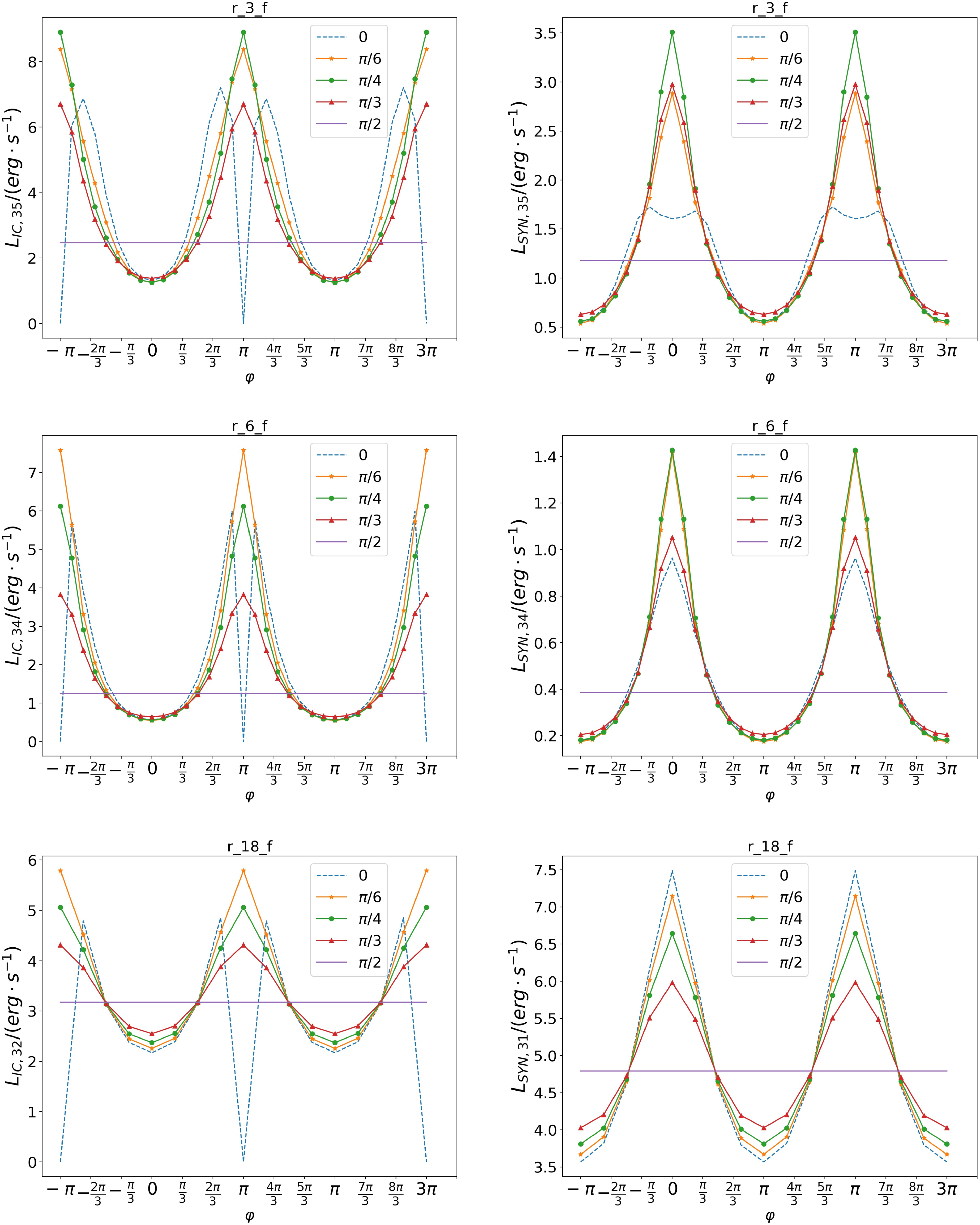
) in the ‘Frisbee’ configuration for five different angles of inclination were constructed: 0o, 30o, 45o, 60o, and 90o (see Fig. 17). The angle of
 $\varphi $
varies from
 $-\pi $
to
 $3\pi $
, describing two periods of rotation of a neutron star. From the constructed light curves the luminosity of the system does not change for SYN and IC radiation for an angle of inclination equal to 90o. This is due to the fact that the binary system does not change its spatial position for the observer. The steepest figures are obtained when the angle of inclination is 0o (the binary system is located with an edge in relation to the observer). But the minimum of IC radiation is observed at the points where the neutron star is located behind a massive star (
 $\varphi = 0$
and
 $\varphi = 2\pi $
), which is associated with photon–photon absorption.
Emissivity maps for IC process with
 $\eta $
= 1/4 (left column),
 $\eta $
= 1/25 (central column), and
 $\eta $
= 1/289 (right column). At the first row ‘Frisbee’ for line of sight along Y-axis, the ‘Frisbee-Bullet’ for lines of sight along X-axis and Y-axis on the second and third rows, respectively, and at the fourth row ‘Bullet’ for line of sight along Y-axis.
Emissivity maps for SYN process with η = 1/4 (left column), η = 1/25 (central column), and η = 1/289 (right column). At the first row ‘Frisbee’ for line of sight along the Y-axis, the ‘Frisbee-Bullet’ for lines of sight along the X-axis and the Y-axis on the second and third rows, respectively, and at the fourth row ‘Bullet’ for line of sight along Y-axis.
Luminosity maps depending on the polar (θ) and azimuthal (φ) angles for the models with η = 1/4 (left column), η = 1/25 (central column), and η = 1/289 (right column). At the first row ‘Frisbee’ IC process and the second row SYN process, the ‘Frisbee-Bullet’ IC process and SYN process on the third and fourth rows, respectively, and the ‘Bullet’ IC process and SYN process on the fifth and sixth rows, respectively.
Parameters of the binary system LS 5039.
Pulsar luminosity on the model.

The dependence of luminosity on the orbital angle of a neutron star for a certain type of radiation (IC and SIN) for six different angles of
 $\theta $
: 0,
 $\pi $
/6,
 $\pi $
/4,
 $\pi $
/3, and
 $\pi $
/2. The orbital angle
 $\varphi $
varies from
 $-\pi $
to
 $3\pi $
, where the angle
 $\varphi $
= 0 means the direction to the observer.
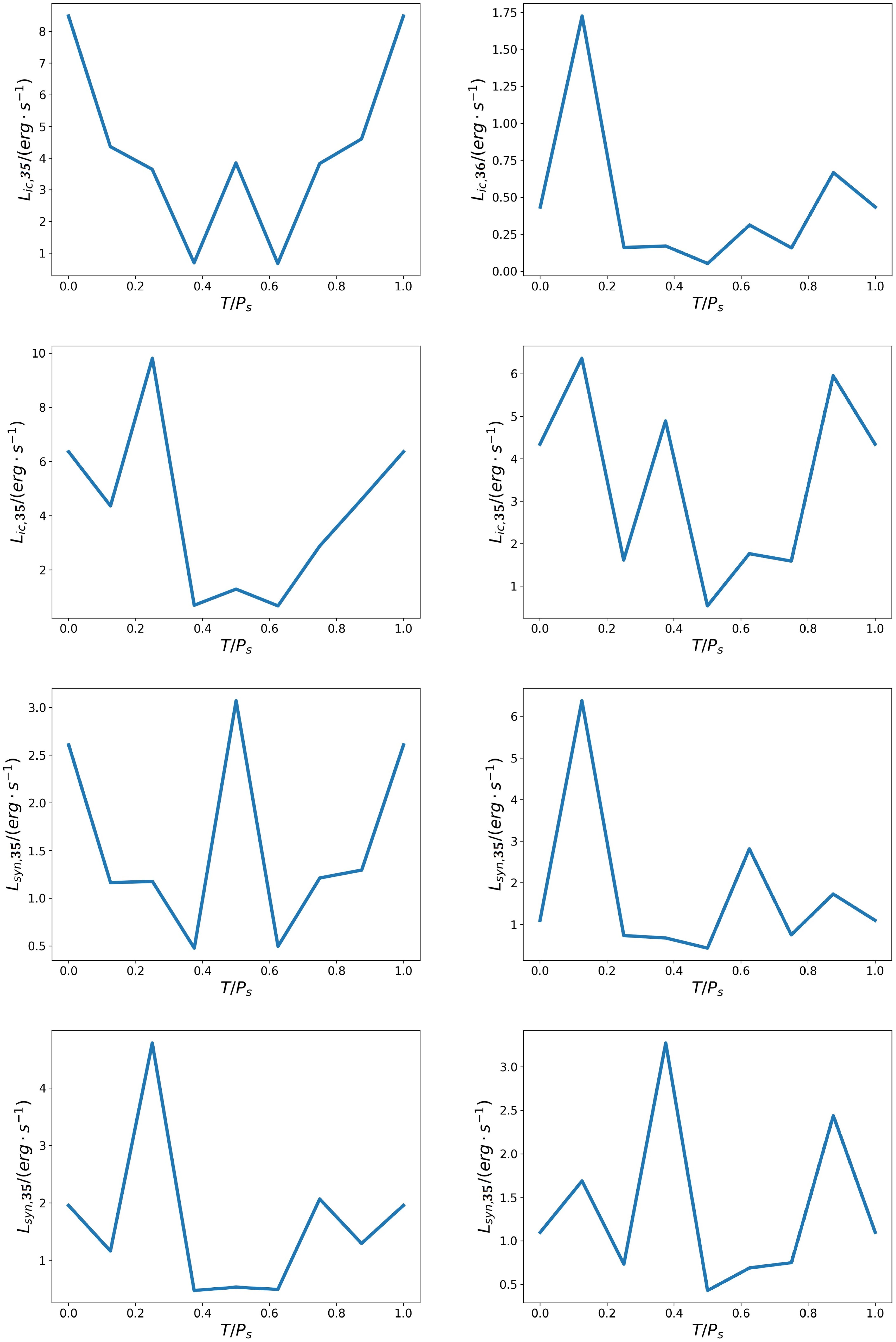
Light curves of equatorial plane of the processes IC (first and second rows) and SYN (third and fourth rows) for η = 1/4. The time is normalised to the period of the orbital motion of the neutron star. The configuration changes as ‘Bullet’ – ‘Frisbee-Bullet’ – ‘Frisbee’ – ‘Frisbee-Bullet’ – ‘Bullet’ every half period. In the first and third rows, the initial configurations are ‘Bullet’ – ‘Frisbee-Bullet’ for the left column or ‘Frisbee-Bullet’ – ‘Bullet’ for the right column. In the second and fourth rows, the initial configurations are ‘Frisbee’ – ‘Frisbee-Bullet’ for left column or ‘Frisbee-Bullet’ – ‘Frisbee’ for right column. At the moment T = 0, the neutron star is located in an infer-far conjunction between the massive star and observer.
If the observer’s line of sight changed only with a change in the angle of
 $\varphi $
, then the luminosity of the system may also differ for the upper and lower parts. This can be seen from the Fig. 16. For ‘Frisbee’ and ‘Frisbee-Bullet’ configurations, such flights in the upper part (
 $\theta $
from 0 to
 $\pi /2$
) would almost not differ from the flight in the symmetrical lower part of the system (
 $\theta $
from 0 to
 $-\pi /2$
, respectively). But at the same time, the flyby from above and from below in the same area (symmetrical points relative to the equatorial plane) are significantly different. So, for example, for the ‘Frisbee-Bullet’ configuration, this difference can reach 100% for SYN and 120% for the IC process. In case ‘Bullet’, the deviation of the jets noticeably affects the luminosity maps (fifth and sixth rows in the Fig. 16), which also affects the flight around the system in the upper and lower parts. It can be seen that with a lower value of the
 $\eta $
parameter (
 $\eta $
= 1/289), the picture remains symmetrical with respect to the orbital plane (
 $\theta $
= 0), but for large values of the
 $\eta $
parameter (
 $\eta $
= 1/4), the difference in the luminosity of the upper and lower parts is noticeable.
Although the described configurations have a static appearance for a certain orientation of the spin of a neutron star, it is possible to construct the light curves of the system under consideration from the obtained results. All these configurations indicate different locations of the neutron star relative to the massive star during rotation. Knowing the angular velocity
 $\omega $
of the orbital motion of a neutron star and using a map of luminosity (Fig. 16) with certain line of sight (which is described by angles
 $\theta $
and
 $\varphi $
), it is possible to determine the time from the formula
 $t\; = \;\alpha /\omega $
, where the angle
 $\alpha $
(in radians) is the phase of the orbital rotation.
If the spin of the neutron star is perpendicular to the orbital plane (‘Frisbee’), then this orbital angle
 $\alpha $
will be the angle
 $\varphi $
from Fig. 16, and the light curve coincides with luminosity maps with fixed value of angle
 $\theta $
. Thus, to construct the light curve in the case of the Frisbee configuration, it is sufficient to select a certain angle of view
 $\theta $
for rows five and six of Fig. 16 and to obtain the dependence of luminosity on the orbital angle
 $\varphi $
. The light curves for the ‘Frisbee’ configuration are shown in Fig. 17. If the spin lies in the orbital plane, there will be a change of configurations ‘Bullet’ – ‘Frisbee-Bullet’ – ‘Frisbee’ – ‘Frisbee-Bullet’ – ‘Bullet’ every half of the period of movement around a massive star; therefore, in addition to the angle of
 $\varphi $
, one need to use different luminosity maps (different rows of Fig. 16). In this case, the configurations ‘Bullet’ and ‘Frisbee’ occur every half of the period, which corresponds to a change in the value of angle
 ${\varphi _0}$
to angle
 ${\varphi _0} + \pi $
, while the configuration ‘Frisbee-Bullet’ is obtained every quarter of the period, which corresponds to a change in angle
 ${\varphi _0}$
to angle
 ${\varphi _0} + \pi /2$
. Fig. 18 shows these light curves for a fixed distance between neutron and massive stars (
 $\eta $
= 1/4). Eight different configurations of a neutron star (8 points on the graph) were used for plotting, which were connected using linear interpolation. The position when the neutron star is located in the infer-far conjunction in front of the massive star is taken as the beginning of the countdown. The figures differ in the initial configuration − the possible direction of the spin of the neutron star relative to the orbital moment. The time is normalised for the orbital motion period P
s
, which for the LS5039 system is P
s
= 3.9d. It can be seen what, in some situations, the light curve for this system can change 8–10 times for a period.
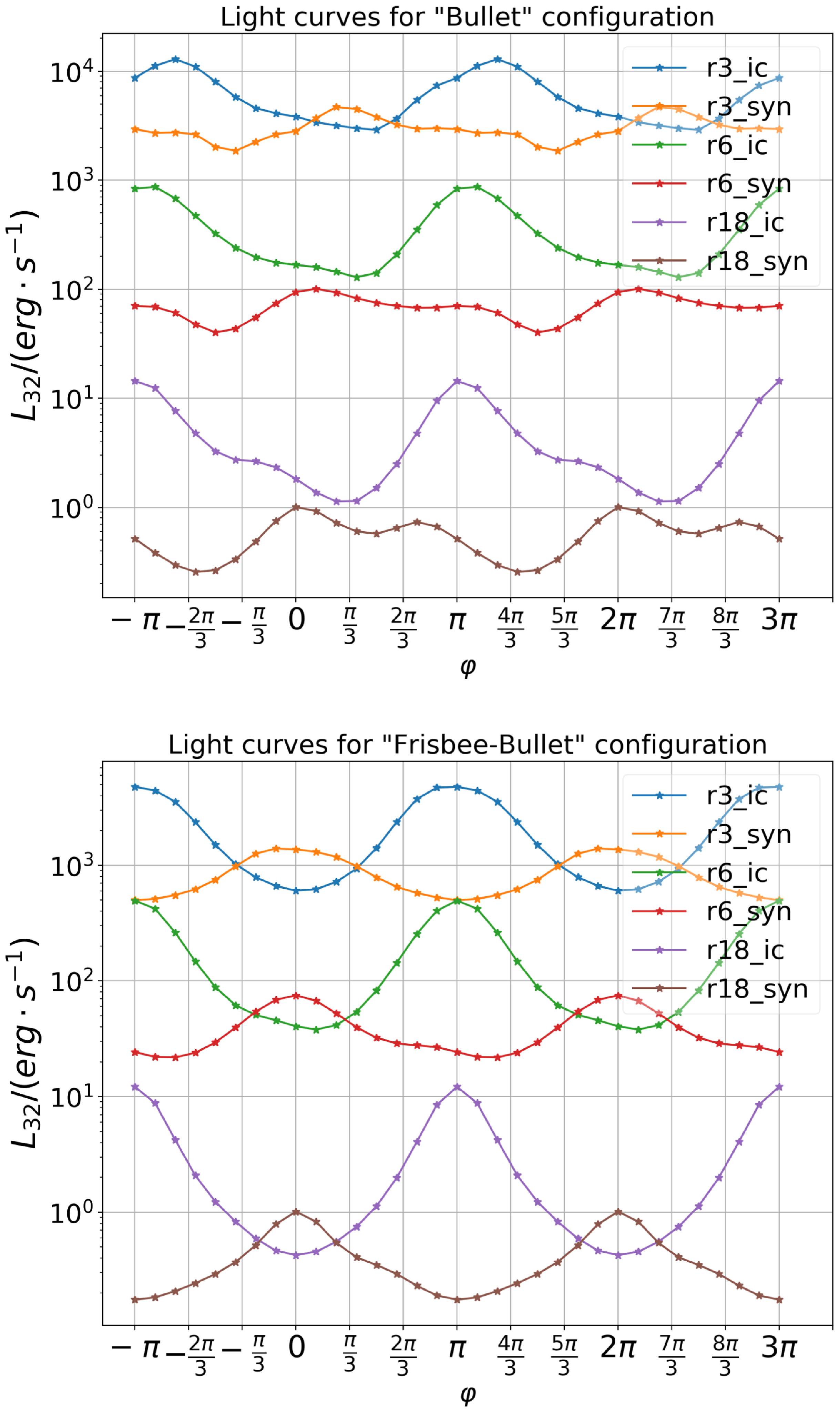
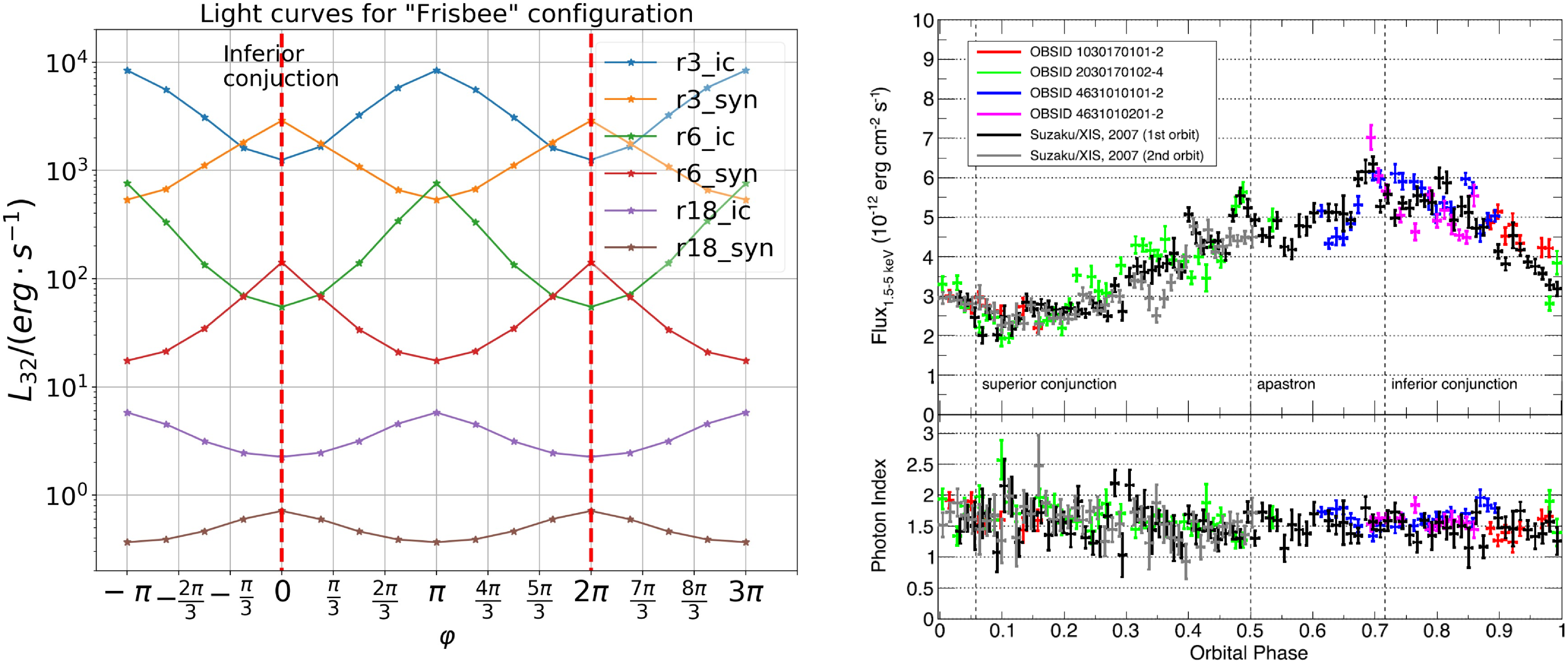
On the Fig. 19 As we can see IC and SYN typical light curves behave in opposite directions. Maximum in the SYN corresponds to minimum in the IC and corresponds to inferior conjunction. We plot theoretical light curves for SYN and IC emission on Fig. 20 and observed X-ray energy band light curve for LS 5039 (Yoneda et al. Reference Yoneda, Bosch-Ramon, Enoto, Khangulyan, Ray, Strohmayer, Tamagawa and Wadiasingh2023). Nether the less LS 5039 system has small eccentricity, the peaks are reached in the inferior conjunction in both cases.
Light curves of
 $\theta = \pi /6$
for different types of configurations: ‘Bullet’ (top panel) and ‘Frisbee-Bullet’ (bottom panel). The figure has six light curves, which has changed the
 $\eta $
-parameter ( = 1/4 for r3,
 $\eta $
= 1/25 for r6, and
 $\eta $
= 1/289 for r18) and types of radiation (SYN or IC). The orbital angle
 $\varphi $
changes from
 $-\pi $
to
 $3\pi $
. The
 $\varphi \;$
= 0 corresponds to the neutron star inferior conjunction.
Light curves of
 $\theta $
=
 $\pi $
/6 for ‘Frisbee’ configuration on the left and LS5039 X-ray observed light curve on the right (we take Fig. 1 from Yoneda et al. Reference Yoneda, Bosch-Ramon, Enoto, Khangulyan, Ray, Strohmayer, Tamagawa and Wadiasingh2023). The left panel has six light curves, which has changed the
 $\eta $
-parameter (
 $\eta $
= 1/4 for r3,
 $\eta $
= 1/25 for r6, and
 $\eta $
= 1/289 for r18) and types of radiation (SYN or IC). The orbital angle
 $\varphi $
changes from
 $-\pi $
to
 $3\pi $
. The
 $\varphi $
= 0 corresponds to the neutron star inferior conjunction.
5. Discussion and conclusion
In this work, we perform numerical relativistic MHD simulations of the wind–wind interaction in gamma-ray binaries. Qualitatively, our results connect previous hydrodynamical simulations of the wind–wind interaction of Bogovalov et al. (Reference Bogovalov, Khangulyan, Koldoba, Ustyugova and Aharonian2008) and magnetised pulsar wind−ISM cases (Bogovalov et al. Reference Bogovalov, Khangulyan, Koldoba, Ustyugova and Aharonian2019; Barkov et al. Reference Barkov, Lyutikov and Khangulyan2019a).
Our 3D simulations demonstrate that the wind–wind interaction in the gamma-ray binaries is different in many respects both from the fluid case and the pulsar wind−ISM cases. We find several features that are specific to 3D (R)MHD simulations that were naturally missed in the previous 2D RMHD work (see Bogovalov et al. Reference Bogovalov, Khangulyan, Koldoba, Ustyugova and Aharonian2012, Reference Bogovalov, Khangulyan, Koldoba, Ustyugova and Aharonian2019). The two-dimensional simulations mostly investigated the dependence of the flow shape on the thrust ratio η (Bogovalov et al. Reference Bogovalov, Khangulyan, Koldoba, Ustyugova and Aharonian2008). As we demonstrate here, the geometry of the pulsar wind is most important.
If compared with the wind–ISM interaction (Bogovalov et al. Reference Bogovalov, Khangulyan, Koldoba, Ustyugova and Aharonian2019), the main difference is the structure of the tail region of the PWN − in the case of planar ISM flow the pulsar wind always terminates at a tailward Mach disc, while in the wind–wind case the pulsar wind may extend to large distances (of the order of several orbital separation). For example, Fig. 3, right column, shows that for a fixed
 $\eta $
the configuration changes from open to closed depending on the geometry of the flow.
In Fig. 6, we show the evolution of the RS opening angle
 $\theta $
depending on the parameter
 $\eta $
and the pulsar orientation angle
 $\zeta $
. Our dependence on
 $\eta $
is generally consistent with the fluid case (Bogovalov et al. Reference Bogovalov, Khangulyan, Koldoba, Ustyugova and Aharonian2008). For 2D MHD simulations Bogovalov et al. (Reference Bogovalov, Khangulyan, Koldoba, Ustyugova and Aharonian2019), found significant decrease of the opening angle with increasing magnetisation of the pulsar wind. For
 $\eta = 0.3$
and
 $\sigma = 0$
,
 $\theta \approx 1$
, then for
 $\sigma = 0.8$
,
 $\theta \approx \;0.35$
. Such the value is close to our ‘Frisbee-Bullet’ orientation case. On the other hand, the bullet orientation trends to significantly wider RS angle, but ‘Frisbee/Cartwheel’ in opposite trends to narrower opening angle, especially in directions in between pulsar spin axis and its equatorial plane. The jet in normal star direction in bullet configuration pushes away CD and did not allow the RS zone to close up to
 $\eta $
> 1/300, which is significantly larger compared to the non-magnetised case
 $\eta $
> 1/50.
Similar tendencies are observed in the closed configurations of pulsar wind (see Fig. 7). The non-magnetised axisymmetric wind forms longer tail compare to ‘Frisbee/Cartwheel’ or ‘Frisbee-Bullet’ configuration, perhaps similar to strongly magnetised wind. The bullet configuration did not form a closed configuration for our set-up. In bullet configuration, jet-like structures push away the FS and reflect stellar wind like umbrella, so it decreases the wind gas pressure in the tail.
Our simulations do not take the dynamics effects of the orbital motion into account − only as a static sequence of different geometries. We can interpret our results as different individual binary systems with various instantaneous orientation of spin axis respect to orbital plane and with respect to the direction towards the companion: (i) if the pulsar spin axis is normal to the orbital plane, we have ‘Frisbee’ configuration all the time; (ii) if the pulsar spin axis lay in the orbital plane, we have ‘Cartwheel’ – ‘Frisbee-Bullet’ – ‘Bullet’ – ‘Frisbee-Bullet’ – ‘Cartwheel’ every half of the orbit; (iii) if the pulsar spin axis angled on 45o to the orbital plane we have transition
‘Frisbee’ – ‘Frisbee-Bullet’ – ‘Frisbee’ every half of the orbit. Thus, taking into account the anisotropic pressure effects of the magnetic field in the pulsar wind leads not only to formation of less compressible outflow in the shocked region, but formation of significantly different flow shape.
We demonstrate that the orientation of the pulsar’s spin axis plays a significant role in the geometry of the shocked pulsar wind. For example, if the pulsar rotation axis lay in the orbital plane, then the length of the free pulsar wind zone can change during 1/4 of the orbit almost one order of magnitude. This can significantly change the emission for the distant observer. We hypothesise that this can be a crucial factor for TeV emission in gamma-ray binaries that suffer from strong photon–photon absorption, up to factor 10 (Khangulyan et al. Reference Khangulyan, Aharonian and Bosch-Ramon2008; Zabalza et al. Reference Zabalza, Bosch-Ramon, Aharonian and Khangulyan2013). Change in the absorption will drastically affect the light curves as well as spectra of such systems.
In the second stage, which is much more numerically challenging, we plan to conduct full 3D relativistic MHD simulations of the orbital motion of the pulsar. Here are the effects of the Coriolis and centrifugal forces becomes important. In the case of seemingly open tail configurations, eventually, at a distance comparable to the orbital separation, the wind zone will be closed due to Coriolis effects (see Bosch-Ramon & Barkov Reference Bosch-Ramon and Barkov2011; Bosch-Ramon et al. Reference Bosch-Ramon, Barkov, Khangulyan and Perucho2012). Even at the present set-up, modelled light curves show feasible behaviour, see Fig. 20. The modelling of the orbital effects should make light curves more asymmetric and closer to observed one. Also, the inclination of pulsar’s rotation axis can be significant, the ‘Frisbee-Bullet’ configuration, that can lead to more smooth and asymmetric light curve formation.
Acknowledgement
The simulations were performed on CFCA XC50 cluster of National Astronomical Observatory of Japan (NAOJ) and RIKEN HOKUSAI Bigwaterfall.
Funding statement
This research was supported by grant NASA 80NSSC20K1534 and 23-22-00385 of the Russian Science Foundation.
Competing interests
None.
Data availability statement
The data underlying this article will be shared on reasonable request to the corresponding author.
Appendix A. Pulsar wind structure
It was assumed that the alternating components of the magnetic field in its striped zone were completely dissipated along its way. Possibly the dissipation has place at the termination shock, but it is not changing the dynamics of the flow see Lyubarsky (Reference Lyubarsky2003). For the total energy flux density of the wind, we adopt the monopole model (Michel Reference Michel1973):
 \begin{align}{f_{tot}}\left( {r,{{\rm{\theta }}_p}} \right) = {L_0}{\left( {\frac{1}{r}} \right)^2}\left( {{{\sin }^2}{\theta _p} + {\rm{g}}} \right),\end{align}
to avoid vanishing energy flux at the poles, we add the parameter
 $g$
= 0.03. This energy is distributed between the magnetic fm component:
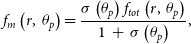 \begin{align}{f_m}\left( {r,{\rm{\;}}{\theta _p}} \right) = \frac{{\sigma \left( {{\theta _p}} \right){f_{tot}}\left( {r,{\rm{\;}}{\theta _p}} \right)}}{{1{\rm{\;}} + {\rm{\;}}\sigma \left( {{\theta _p}} \right)}},\end{align}
and kinetic
 ${f_k}$
one
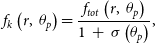 \begin{align}{f_k}\left( {r,{\rm{\;}}{\theta _p}} \right) = \frac{{{f_{tot}}\left( {r,{\rm{\;}}{\theta _p}} \right)}}{{1{\rm{\;}} + {\rm{\;}}\sigma \left( {{\theta _p}} \right)}},\end{align}
where
 $\sigma \left( {{\theta _p}} \right)$
is wind magnetisation, which depends on latitude, the angle
 ${\theta _p}$
) is counted from the pulsar spin axis.
For numerical stability magnetisation is vanishing at the pole region as:
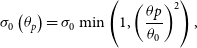 \begin{align}{\sigma _0}\left( {{\theta _p}} \right) = {\sigma _0}\min \left( {1,{{\left( {\frac{{\theta p}}{{{\theta _0}}}} \right)}^2}} \right),\end{align}
where
 ${\theta _0}$
is another small parameter which is equal to 0.2. The magnetic stripes dissipation changes the wind magnetisation at the equatorial zone as:
 \begin{align}\sigma \left( {{\theta _p}} \right) = \frac{{{\sigma _0}\left( {{\theta _p}} \right){\chi _\alpha }\left( {{\theta _p}} \right)}}{{1{\rm{\;}} + {\rm{\;}}{\sigma _0}\left( {{\theta _p}} \right)\left( {1{\rm{\;}}-{\rm{\;}}{\chi _\alpha }\left( {{\theta _p}} \right)} \right)}},\end{align}
where
 \begin{align}{\chi _\alpha }\left( {{\theta _p}} \right) = \left\{\begin{array}{l@{\quad}l} \left( {2{\phi _\alpha }\left( {{\theta _p}} \right)/\pi - 1} \right)^2, & \frac{\pi}{2}-\alpha < {\theta _p} < \frac{\pi}{2} + \alpha \\ 1, & otherwise\end{array}\right.,\end{align}
and
 ${\phi _\alpha }\left( {{\theta _p}} \right) = {\rm{arccos}}\left( {-{\rm{cot}}\left( {{\theta _p}} \right){\rm{cot}}\left( \alpha \right)} \right)$
. The
 $\alpha $
is the angle between the magnetic axis and the pulsar rotation axis (see for more details in Komissarov Reference Komissarov2013).
Appendix B. Radiation processes and Doppler boosting
The main non-thermal processes dominating the radiation of the interaction of winds are the synchrotron (SYN) and the inverse-Compton (IC). To quantify these processes, cooling times are calculated.
For electrons interacting with stellar photons due to IC process, a characteristic cooling time is used (Bosch-Ramon & Khangulyan Reference Bosch-Ramon and Khangulyan2009; Khangulyan, Aharonian, & Kelner Reference Khangulyan, Aharonian and Kelner2014; Barkov & Bosch-Ramon Reference Barkov and Bosch-Ramon2018), expressed as:
 \begin{align}{t_{IC}} = \gamma /{\dot \gamma _{IC}},\end{align}
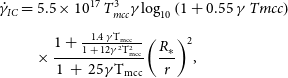 \begin{align}{\dot \gamma _{IC}} & = 5.5 \times {10^{17}}{\rm{\;}}T_{mcc}^3\gamma {\log _{10}}\left( {1 + 0.55{\rm{\;}}\gamma {\rm{\;}}Tmcc} \right)\nonumber\\[5pt]& \quad\times \frac{{1 + \frac{{1.4{\rm{\;\gamma }}{{\rm{T}}_{{\rm{mcc}}}}}}{{1{\rm{\;}} + {\rm{\;}}12{{\rm{\gamma }}^2}{\rm{T}}_{{\rm{mcc}}}^2}}}}{{1{\rm{\;}} + {\rm{\;}}25{\rm{\gamma }}{{\rm{T}}_{{\rm{mcc}}}}}}{\left( {\frac{{{R_{\rm{*}}}}}{r}} \right)^2},\end{align}
where
 $\gamma $
is the electron Lorentz factor,
 ${T_{mcc}} = k{T_*}/{m_e}{c^2}$
, the stellar temperature in electron rest energy units,
 ${R_*}$
the stellar radius, and r the distance to the star from the radiating region.
For SYN radiation, the time characteristic has the form:
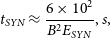 \begin{align}{t_{SYN}} \approx \frac{{6 \times {{10}^2}}}{{{B^2}{E_{SYN}}}},s,\end{align}
where B is the magnetic field in G, and
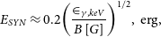 \begin{align}{E_{SYN}} \approx 0.2{\left( {{{{ \in _{\gamma, keV}}} \over {B\left[ G \right]}}} \right)^{1/2}},{\rm{\;erg}},\end{align}
The characteristic value of the emissivity of one calculation cell can be estimated as
 ${u_{cell}}/{t_{rad}}$
, where
 ${u_{cell}} = 3P$
and subscript ‘rad’ means SYN or IC. But to calculate the luminosity of the entire system, it is necessary to sum up the resulting value over the entire volume
 ${L_{rad}}\;~\mathop \smallint \nolimits_V \left( {{u_{cell}}/{t_{rad}}} \right)dV\;\;$
.
The obtained values refer to the radiation in its own frame of reference. To find quantitative values of the emissivity on the part of the observer (laboratory reference frame), it is necessary to take into account the change in the frequency of the emitted photon
 $\nu ' = \nu /\delta $
and the Doppler boosting, where the Doppler factor is
 $\delta {\rm{\;}} = 1/\Gamma \left( {1-\beta {\rm{\;cos}}{\theta _{obs}}} \right),{\rm{\;}}\beta = v/c$
and
 ${\theta _{obs}}$
is the angle between the directions of the observer and the motion of commoving frame of plasma. The detailed procedure of Doppler boosting calculation was taken from (Barkov, Lyutikov, & Khangulyan Reference Barkov, Lyutikov and Khangulyan2019).



