


1. Introduction
This research note presents a new dataset of largely comparable and consistently defined series on wage inequality in manufacturing in Argentina, Brazil, Chile, Colombia, Mexico, and Venezuela (LA6) from 1920 to 2011. There are also series of reduced comparability in a wider sectoral sample of unskilled labor. This resource can be useful to researchers studying the process of modernization and industrialization in the region, as well as the dynamics of wage dispersion of unskilled workers during a period of significant internal migration and urbanization.Footnote 1 Wage inequality is measured by the coefficient of variation (cv) and by the white-collar premium (i.e., the white- to blue-collar wage ratio). I am using these simpler measures instead of more comprehensive inequality indicators such as the Gini and Theil coefficients because their lower data demands allow for a greater number of observations. However, trajectories based on the three measures tend to coincide.
The dataset spans a period that captures developments over three subperiods characterized by distinctive economic growth and development strategies. Roughly speaking, 1920–1939 includes the transition years that followed the end of the First Globalization; 1940–1979 comprises the core years of state-led, protected industrialization (SLPI); and 1980–2011 covers an episode of export-led growth (ELG) and neoliberal reforms—starting earlier in the 1970s in Chile and Argentina. These data compilations build on the work of Ewout Frankema (Reference Frankema2012) in two ways. First, literally, since he generously shared with me his dataset of digitalized industrial censuses and surveys, which, for the LA6, I considerably expanded, complemented, and extended into the 2010s.Footnote 2 Secondly, by providing the theoretical foundations and the Latin-American historical context in which to place my work.
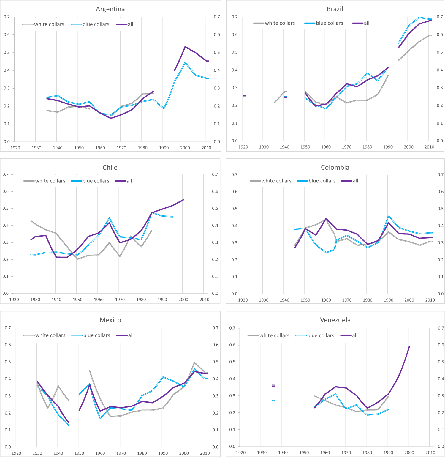
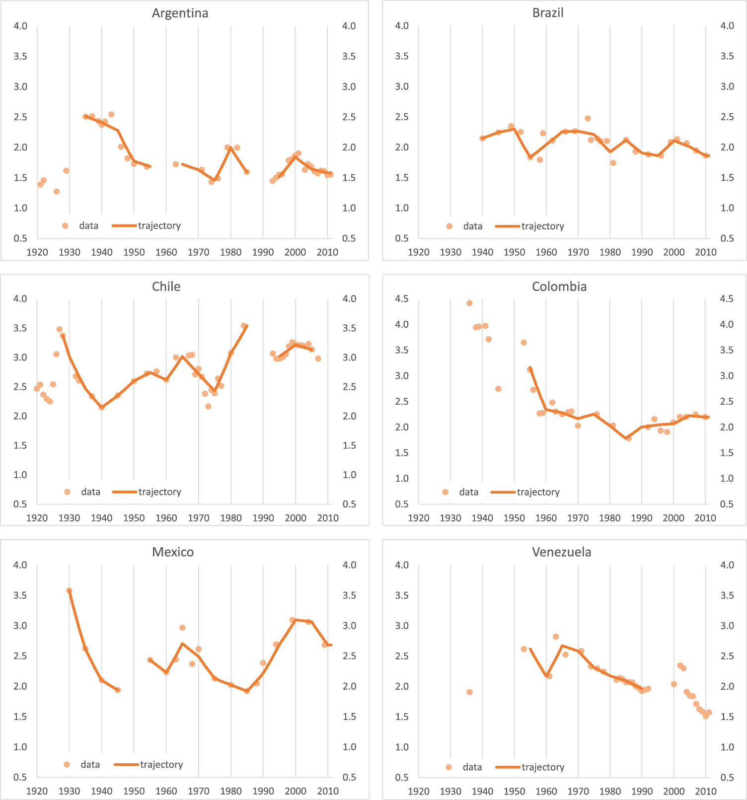
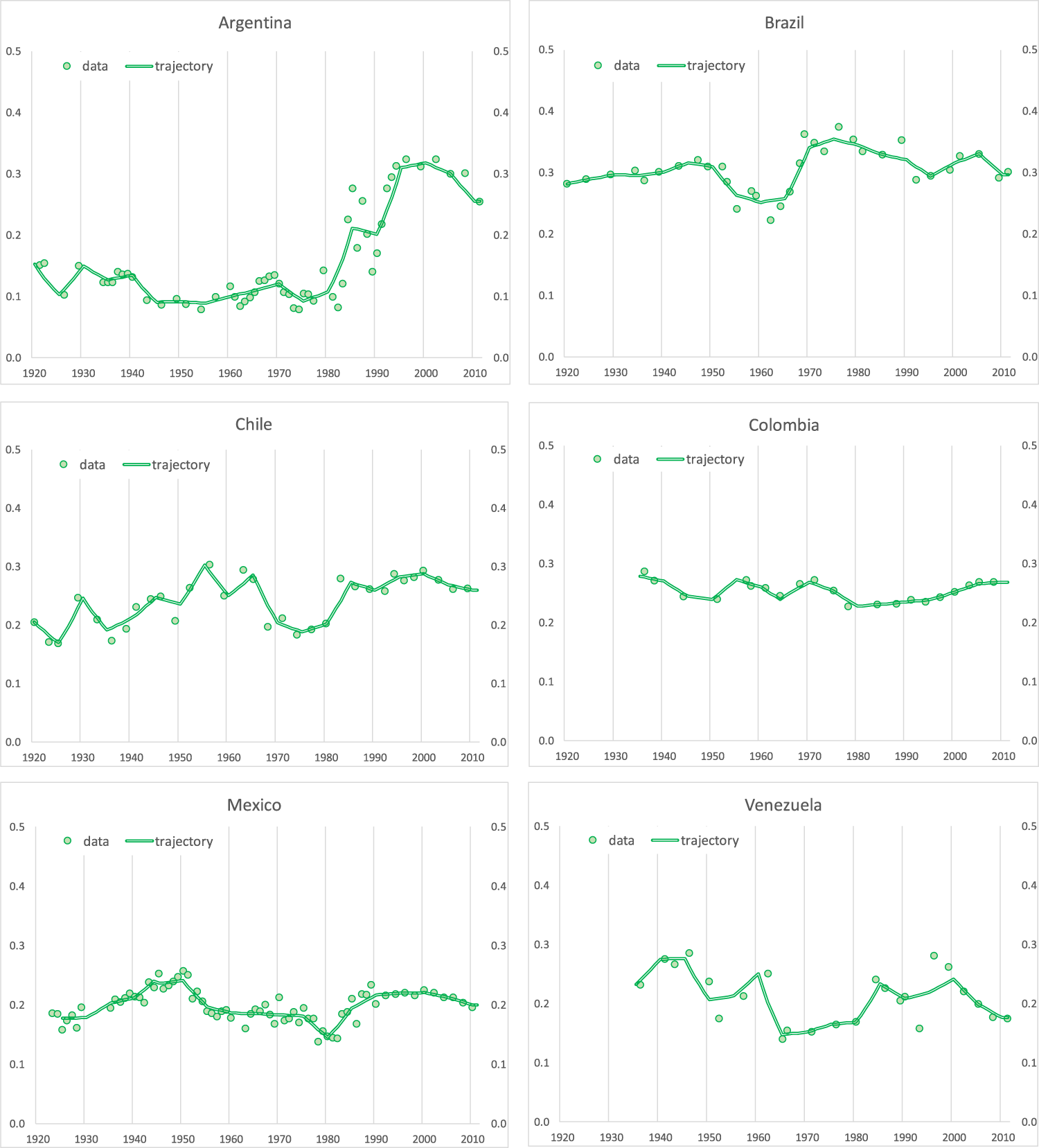
The dataset includes series of inter-industry wage dispersion in overall manufacturing (cvall) and the breakdown into white- and blue-collar categories (cvwc, cvbc). Data points are presented together with trajectories based on averages every five years. See Figure 1 with summary of trajectories of cvall, cvwc, cvbc, and Figures OA.1, OA.2, OA.3 in the Online Appendix with full details by country. It also incorporates white-collar premiums for years in which there are comparable data for both categories (Figure 2). These are complemented by intra-industry premiums in benchmark years according to the International Standard Industrial Classification Rev.1 (ISIC1), together with the corresponding white-collar labor shares (Figures OA.4 and OA.5 in the Online Appendix). Beyond manufacturing, there are series of wage dispersion for unskilled occupations (cvunsk) in the wider economy (Figure 3) which, when possible, take into account the urban-rural divide.Footnote 3
Trajectories in wage dispersion in manufacturing.

White-collar wage premiums.

Wage dispersion of unskilled workers.

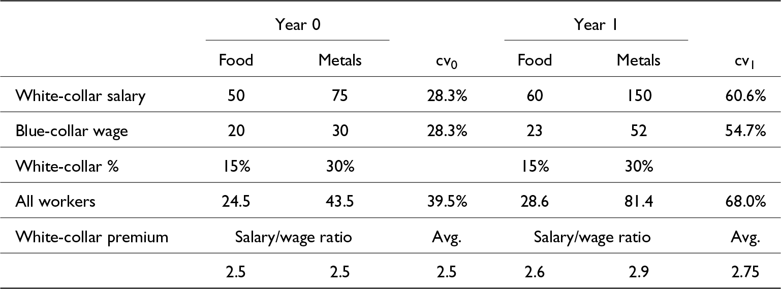
Table 1 clarifies the connection between the series in manufacturing. It is assumed that there are two industries, “food” and “metals,” which produce goods that are relatively intensive in the use of labor and capital, respectively. For “Year 0” and “Year 1,” basic information is presented on the mean salary and wage paid in each industry, along with their respective labor share of white-collar workers (white-collar %). Consistent with the evidence, it is assumed that the metal industry pays higher salaries and wages due to its higher productivity and has a higher percentage of white-collar workers. Between the two years, there is an expansion of both industries, which, due to productivity differences, results in a widening of inter-industry wage dispersion (cv 1 > cv 0) and higher intra-industry white-collar premiums. In the situation depicted in the table, the levels of wage dispersion for “all workers” are above those of white and blue collars, which broadly reflects the LA6 evidence.
Links between inequality series in manufacturing

Wages for “all workers” are calculated as the weighted average of white-collar salary and blue-collar wage; “avg.” = simple average.
Inter-industry wage dispersion for all workers and white-collar premiums are two key measures of wage inequality. The former reflects average income differences across industries of varying capital intensity and technology-skill content. This is likely to capture differences in labor productivity and technological sophistication (Berman et al., Reference Berman, Bound and Machin1998). The latter looks at income gaps between two labor categories defined by their skill level. Here the emphasis is on the returns to skills given differences in labor productivity and technology.
There are three dominant narratives in the literature studying developments in industrial wage inequality: (i) skill-biased technological change (SBTC), where the production technology favors skilled over unskilled labor by increasing its relative productivity (Goldin and Katz, Reference Goldin and Katz1998; Acemoglu, Reference Acemoglu2002); (ii) (de)globalization (Freeman, Reference Freeman1995), where the assumption of factor price equalization plays a prominent role in interpreting movements in wage gaps across countries; and (iii) institutions including (de)unionization, labor-market regulations and minimum wages (Wallerstein, Reference Wallerstein1999).Footnote 4
Empirically, it is difficult to unpack the individual impact of each narrative on patterns of wage inequality, particularly of SBTC and globalization, because they tend to induce changes in the same direction. All in all, in Latin America, the years of SLPI are characterized by SBTC with the promotion of relatively capital-intensive industries, deglobalization, and pro-labor institutions (particularly in Argentina, Chile and Mexico). Regarding the expected effect on inequality in both inter-industry wage dispersion and white-collar premiums of SBTC amid shortages of skilled labor is to widen it. And shielding manufacturing from foreign competition should lead to a similar result. However, labor market regulations, unionization, and the introduction of minimum wages are expected to reduce wage inequality, making the net impact ambiguous in theory.Footnote 5
The following period of ELG up to c.2000 brought about trade liberalization, deregulation (including pay), labor flexibility and a decline in the power of unions, amid the continuation of SBTC driven by innovations in information and communication technology. This time, the net impact of the three narratives is expected to result in a widening of inequality. The 2010s benefited from a commodity boom, creating the conditions for pro-labor policies.
Regarding dispersion in unskilled labor, it is expected to fall in line with the pace of urbanization (due to lower urban-rural wage gaps and an increasing share of urban workers), particularly during those decades with intense flows of internal migration. Dispersion is also likely to decline during years dominated by an active minimum-wage policy which was a feature during SLPI and the 2010s. Overall, minimum wages were eroded during the final two decades of the last century (since the early 1960s in Brazil).
This long-term dataset makes three contributions to the statistics of the region. First, it offers comparable and consistently defined series on wage inequality in manufacturing across the LA6. This is complemented by series of unskilled wage dispersion, though of limited comparability. In both cases, there are enough observations to inform about trajectories and turning points across particular development and growth periods. Secondly, it includes white-collar premiums in manufacturing. This is a basic measure of labor-income inequality in a key sector during SLPI where there is limited comparable evidence. It also provides a reasonable proxy for premiums in the formal sector. Thirdly, the addition of more detailed intra-industry data in a number of benchmark years during the second half of the twentieth century makes it possible to identify patterns and dynamics of interest related to variations in skill premiums and labor shares of white- and blue-collar workers.Footnote 6
A visual inspection of the evidence for manufacturing shows that: First, altogether, the dominant pattern in inter-industry wage inequality is a steady rise starting around 1960 in Argentina, Brazil, and Mexico, in c.1970 in Chile and c.1980 in Colombia (only in the 1980s) and Venezuela. This evidence is consistent with that based on Theil coefficients in Frankema (Reference Frankema2012), which uses fewer observations—Figure OA.1 in the Online Appendix. Secondly, the trajectories of wage dispersion for white- and blue-collar workers, although largely positively correlated, exhibit episodes of divergence, indicating the different impacts of market and institutional forces. Thirdly, SLPI shows falling white-collar premiums across the LA6, indicating a dominant effect of labor institutions; whereas, as expected, widening trends prevail during ELG (Venezuela is the exception) until 2000. The 2010s is a decade of falling premiums likely to be driven by sustained increases in minimum wages (Moreno-Brid et al., Reference Moreno-Brid, Garry and Krozer2016). Fourthly, overall, there is a rise in white-collar labor shares over time consistent with SBTC.
Regarding the dispersion of unskilled wages, there are two patterns to highlight. First, when there is evidence of the rural-urban divide, there are falling trajectories in Brazil (1950 to mid-1960s), Colombia (1940 to 1980, with interruptions), and Mexico (1950 to 1980), consistent with the combined action of urbanization and minimum wages. Secondly, in times of highly urbanized populations, the 1980s and 1990s are dominated by rising trends in all countries except Brazil; whereas falling trends prevail in the 2010s. These contrasting trends are likely to be driven by a reversal in labor-market policies, particularly in minimum wage policies.
2. About the series
The data on manufacturing come from official industrial censuses and surveys in most cases following the ISIC breakdown by industries (divisions) at the national level; and from two international statistical compilations: the United Nations Yearbook of Industrial Statistics (UN YIS) and the International Labour Organization Yearbook of Labour Statistics (ILO YLS). Differences in skills are captured by the separation of white and blue-collars across industries. Data up to the 1980s usually refer to ISIC1 (20 industries), and to ISIC Rev. 2 (ISIC2, 28 industries) thereafter. The comparison of cvs across industries shows that discrepancies between ISIC1 and ISIC2 in benchmark years are relatively small (in most cases within a ±5% interval).
Unfortunately, the advantage of having one source with a homogeneous breakdown of wage data at a national level is lacking for unskilled workers in the broader economy. This poses an estimation challenge, making it necessary to splice a series of different sources and geographical, sectoral, and occupational coverage. One key resource is comparable urban wages across countries in a selection of unskilled jobs in manufacturing, construction, and services from the International Labour Organisation’s October Inquiry.Footnote 7 In recent decades, if necessary, I use income dispersion at the lower section of the distribution as reported in official household budget surveys (HBS). As I am covering a period of rapid internal migration, a key issue is the urban-rural divide. To capture its impact on wage dispersion, where data allow, I assembled a representative sample of unskilled wages for rural and urban occupations in benchmark years, with the proportions reflecting the urbanization rate at the time. In Brazil and Colombia, I accounted for wage disparities within and between both sectors. In Mexico, due to limited rural wage data, the series includes both within-urban dispersion and the urban-rural wage gap.Footnote 8 In Argentina and Chile, with significant urban population already in the 1920s, dispersion is urban driven. This is also the case in Venezuela where rural-wage data are scarce.
Due to the challenges in gathering comprehensive and consistently defined data on unskilled wages across the LA6 and over time, this evidence is necessarily of mixed quality. Data accuracy is also compromised by the dominance of informal activities among the unskilled, which tend to be underestimated in the data. This means reduced comparability on dispersion levels across countries. However, importantly, this evidence should inform about changes in countries’ trajectories.
3. Procedure and sources by country
This section describes the sources used and the procedure followed to assemble the series of wage inequality. It starts with manufacturing and ends with unskilled labor.
3.1. Manufacturing
For each country, there is information on wage dispersion for blue-collar workers (cvbc), white-collar workers (cvwc), all workers (cvall), and white-collar premiums. When possible, premiums for the entire manufacturing sector are calculated using totals of salaries, wages, white-collar, and blue-collar employees (i.e., total salaries per white-collar employee divided by total wages per blue-collar employee). The comparability of these “aggregate premiums” is not affected by differences in the industry breakdown. It also has the advantage of minimizing data demands. When those totals are not available, I calculated the overall premiums by averaging individual intra-industry values, which I refer to as “average premiums” (see Table 1). In general, differences between both outcomes tend to be within the ±10% interval.
3.1.1. Argentina
Blue collars: In 1921/22, 1926, 1929 daily wages for unskilled and semi-skilled male workers in 10 manufacturing industries in Buenos Aires city (Shipley, Reference Shipley1977, Table IX-A). The industry breakdown of these early data and their geographical coverage are not compatible with the Industrial Census of 1935 (Comisión Nacional del Censo Industrial—CNCI, 1938), which covered 16 industries at the national level. Industrial censuses in 1946 (Dirección General del Servicio Estadístico Nacional—DGSEN, 1952), and 1950, 1954, 1963(ISIC1) from DNEC (Dirección Nacional de Estadística y Censos—DNEC, 1957, 1960, 1968); 1974 (ISIC2), 1985 from UN YIS (United Nations—UN, 1975–2006, 1986). Industrial surveys in 1937, 1941 from (Dirección General del Servicio Estadístico Nacional—DGSEN, 1952); 1971 (ISIC2), 1976, 1979, 1982 from UN YIS (United Nations—UN, 1975–2006, 1980; International Labour Organization—ILO, 1964–1982). Owing to a lack of separate data for salaries and wages, the value in 1941 is estimated using salaries and wage shares by industries calculated as the simple average of equivalent shares in 1937 and 1946. A similar procedure is followed in 1950 using shares in 1946 and 1954 (Dirección Nacional de Estadística y Censos—DNEC, 1960). Values in 1960 and 1967 are estimated based on changes in average hourly earnings from ILO YLS (1970, 1980).
1985–2011: In 1989, 1993, 1996, 99, 2002, and 2005, I use changes in hourly earnings from ILOSTAT (International Labour Organization—ILO, 2022) based on three-year averages in the ILO series for each benchmark; and in 2008 and 2010, I use changes in the index of salario por obrero (Instituto Nacional de Estadística y Censos—INDEC, 2024).
White collars: Monthly salaries for white-collar male workers in 10 industries in Buenos Aires city (Shipley, Reference Shipley1977, Table IX-A). Data in 1921 (missing data on chemicals, wood printing, and leather are estimated using the wage structure in 1922), 1922, 1926, and 1929 (excluding tobacco—an outlier). The industry breakdown of these early data and their geographical coverage is not compatible with the Industrial Census of 1935.
1935–1985: There are no observations in 1960 and 1967; otherwise, data years and sources as in cvbc. 1993–2011: I was unable to find sufficient information to calculate the dispersion of salaries.
All workers: Data years and sources between 1935 and 1985 are as in cvbc; except surveys in 1937 (Dirección General del Servicio Estadístico Nacional—DGSEN, 1952) and 1957 (United Nations—UN, 1953–1965). Dispersion of earnings per employee in overall manufacturing in 1993 (ISIC2), 1996, 1998–2001 from UN YIS (1999, 2002, 2006). From 2002 to 2011 it grows with ISIC3 series (Ministerio del Trabajo, Empleo y Seguridad Social de Argentina—MTESS, 2019). No data are reported for the oil and coal industry 1971–1985; but it is included in 1993. This results in a step rise in dispersion of approximately 5 percentage points in 1993, from 41.17% with data on oil and coal to 35.93% without it.
White-collar premiums: Between 1921 and 1929, blue-collar monthly wages are calculated from daily values assuming 24 working days per month. Data years and sources between 1921 and 1929 and 1935–1985 (except 1948) are as in cvbc and in cvwc. Census data in 1948 (Dirección Nacional de Estadística y Censos—DNEC, 1949/50). There are no separate data on salaries and wages in 1948 and 1950. To estimate them, I calculate salaries and wage shares of total manufacturing interpolating equivalent shares in 1946 and 1954.
1993–2001 and 2003–2011: It uses data on blue-collar workers (obreros) and monthly mean wages in manufacturing (Instituto Nacional de Estadística y Censos—INDEC, 2024, Encuesta Industrial Mensual) to calculate blue-collar annual wages, assuming 13 monthly payments. This amount is subtracted from total remunerations (sources as in cvall) to calculate white-collar annual salaries. The dispersion level in 1993 is not fully comparable with that of 1985.
3.1.2. Brazil
Blue collars: Industrial censuses or surveys in 1940 (II Census) from Instituto Brasileiro de Geografia e Estatistica—IBGE (1950), 1950 (III Census—ISIC1) from IBGE (1957); 1952, 1955, 1958, 1962, 1966, 1969 from IBGE (1952–1969); 1973/74, 1976/77, 1979 from UN YIS (1976, 1980, 1982); 1981, 1984/85, 1988, 1992 from IBGE (1972–1992); in 1996 (ISIC3-four digits), 1999, 2001, 2004, 2007, 2010 from IBGE (2022).
White collars: Data in 1937 (18 industries) from IBGE AEB (1938). Data years and sources from 1940 to 2010 are as in cvbc.
All workers: In 1920 it uses wage dispersion in 12 industries from the I Census (Diretoria Geral de Estatistica, 1927). Data in 1970 from UN YIS (1975); otherwise, years and sources from 1940 to 2010 are as in cvwc.
Note: Because of the change from ISIC1 to ISIC3, the dispersion level of cvbc, cvwc, and cvall in 1992 is not fully comparable with that of 1996 and onward.
White-collar premiums: Data years and sources are as in cvbc and cvwc. Interpolation in 1945.
3.1.3. Chile
Blue collars: In 1920–1927 real-wage dispersion in 15 industries (Matus, Reference Matus2009). In 1928 (22 industries), 1937, 1957, 1967 census data from Rodriguez Weber (Reference Rodríguez Weber2014; Tables AE28/28 and AE31/32—ISIC1 matching) excluding employers and self-employed workers. In 1953 (ISIC1) industrial survey from UN (1953–1965). Values in 1932, 1933, 1940, 1945, 1950, 1954, 1960, and 1963 are estimates from Rodriguez Weber (Reference Rodríguez Weber2014).
1968–1984: ISIC1 up to 1972, and ISIC2 up to 1984 from UN (1973) and UN YIS (1975–2006).
1985–1993: It grows with dispersion in monthly earnings in ISIC2 industries (International Labour Organization—ILO, 2022).
White collars: From 1920 to 1984, data years and sources are as in cvbc. 1985–2011: I could not find enough information to calculate dispersion of salaries.
All workers: No employees data in 1927; otherwise, data years and sources in 1920–1984 are as in cvbc. 1985–2005: 1985 (ISIC2), 1989 from UN YIS (1989); and 1992, 1996, 1998, 2000 from United Nations Industrial Development Organization—UNIDO (1996, 2003).
White-collar premiums:
1920–1984: Data years and wage sources are as in cvbc and cvwc. 1993–2005 and 2007: It uses data of remuneraciones medias mensuales por grupos ocupacionales (Instituto Nacional de Estadísticas de Chile—INE, 1993–2007) for white collars and blue collars. The dispersion level in 1993 and onward is not fully comparable with that of 1984.
3.1.4. Colombia
Blue collars: wages in 1936 (22 industries), 1938/39 (25 industries), 1941/42 (Dirección Nacional de Estadística—DNE, 1936, 1942, 1946). The breakdown of these early data is not compatible with that of the First Industrial Census of 1945 (Dirección Nacional de Estadística—DNE, 1947). Industrial censuses or surveys in 1945 (I Census-ISIC1), 1953 (II Census), 1963, 1967, 1970, 1976 (ISIC2), 1981, 1986 from Departamento Administrativo Nacional de Estadística—DANE (2020). In 1950 I use changes in the dispersion of daily males’ earnings in 11 ISIC1 industries (ILO YLS 1949/56) to move backward from the 1953 benchmark.
In 1955, it uses ILO YLS (1963) with the aggregate “chemicals and oil” split using data from the 1953 Census. In 1956, 1958/59 the series grows with wage dispersion in 15 industries from Departamento Administrativo Nacional de Estadística—DANE (1953–1961) from the 1955 benchmark. In 1962 dispersion in hourly earnings in 20 ISIC1 industries from ILO YLS (1976). In 1965 and 1968, the series grows with wage dispersion in 20 ISIC1 industries from Departamento Administrativo Nacional de Estadística—DANE (1962–1968) from the 1963 and 1967 benchmarks. Values in 1971–1975 and 1977–1979 are calculated using changes in daily earnings in 20 ISIC1 industries to move forward from the 1970 and 1976 benchmarks (ILO YLS 1976 & 1980). In 1992, 1994, 1996, 1998 (ISIC2) and 2000, 2002, 2004, 2007, 2010 (ISIC3) from Departamento Administrativo Nacional de Estadística—DANE (1992–2010) with permanent workers only. The 2000 figure is estimated based on the structure of salaries and wages of 2002.
White collars: 1955/56 and 1958/59 data on 15 industries from Departamento Administrativo Nacional de Estadística—DANE (1962–1968). Chemicals and oil products are split using data from the 1953 Census. In 1962, 1965, and 1968, the series grows with salaries dispersion in 20 industries from Departamento Administrativo Nacional de Estadística—DANE (1962–1968). Otherwise, data years and sources are as in cvbc.
All workers: in 1957/58 and 1963 (Departamento Administrativo Nacional de Estadística—DANE, 1962–1968), between 1959 and 1962 it grows with dispersion in remunerations (Departamento Administrativo Nacional de Estadística—DANE, 1970). In 1980 and 1982–85 and 1988–91 it grows with dispersion of monthly earnings per employee (ILOSTAT 2002). Figure in 2000 (ISIC3) is estimated using the structure of 2002 for salaries and wages; otherwise, sources are as in cvwc.
White-collar premiums: data years and sources for 1936–1942 and 1945–1986 are as in cvbc and cvwc. Because of differences in employee coverage, levels of pre-1945 premiums are not compatible with those after 1945. Values in 1936, 1938/39, 1941/42, 1955/56, 1958/59, 62, 65, and 1967/68 are “average premiums.” In 1992–2010 it uses data of blue and white collars for permanent workers only from Departamento Administrativo Nacional de Estadística—DANE (1992–2010). I use the structure of 1994 to split blue and white collars in 1996 and 1998.
3.1.5. Mexico
Blue collars: In 1930, 1935, 1940, 1945 it uses wages in 14 industries from the first four industrial censuses (Dirección General de Estadística—DGE, 1953). I excluded “Artes gráficas, fotografía y cinematografía” because it has a large component of services. In 1955 (ISIC1), 1960, 1965, 1970, and 1975 I used census data (Instituto Nacional de Estadística, Geografía e Informática—INEGI, 2020). To make an estimate in 1950 I grouped hourly wages of 25 activities (Dirección General de Estadística—DGE, 1938–1977) into 14 ISIC1-matching industries and used changes in their dispersion to move backward from the 1955 benchmark. The observation in 1965 uses data from D.F. and Estado de Mexico only—both states accounted for half of manufacturing employment in that year. National industrial surveys are used in 1978, 1981, 1986 (ISIC2 onward), 1988 and 1990 (UN YIS 1990); and census data in 1994, 1998, 2004, and 2009 (Instituto Nacional de Estadística, Geografía e Informática—INEGI, 2020). Observations in 1998, 2004, and 2009 are calculated using changes in ISIC2 four-digits data from the 1994 benchmark.
White collars: No observation in 1950; otherwise, data years and sources are as in cvbc.
All workers: 1950 (ISIC1) from DGE (1957). In 1930, 1935, 1940, 1945, and 1950 calculations include employers. Observations in 1992, 1996, 2000 (United Nations—UN, 1975–2006). Otherwise, data years and sources are as in in cvbc.
Note: Because of differences in industry breakdown, levels of pre-1945 are not fully comparable with those after 1950. Also, because of unusually high values of earnings per employee, observations for petroleum and coal products are excluded in the calculations of cvbc, cvwc, and cvall in 1955 (if included the values would be 41.68%, 57.4%, and 38.1% respectively).
White-collar premiums: Census data in 1965 for all Mexico (Dirección General de Estadística—DGE, 1968). National surveys in 1963 and 1968 (Instituto Nacional de Estadística, Geografía e Informática—INEGI, 2020, Estadística industrial anual). Otherwise, data years and sources are as in cvbc and cvwc.
3.1.6. Venezuela
Blue collars: 1936 (11 industries) from the I Industrial Census (Valecillos, Reference Valecillos1993, p. 27), 1953 (ISIC1) from II Industrial Census (Dirección General de Estadísticas y Censos Nacionales—DGECN, 1961); in 1961, 1966, 1971 industrial surveys from Oficina Central de Coordinación y Planificación—Cordiplan (1963, 1968, 1973). Industrial surveys (ISIC2) in 1974, 1976, 1978, 1982/83, 1985/86, 1989–1992 (Oficina Central de Estadística e Informática—OCEI, 1974–2002).
White collars: Data years and sources are as in cvbc.
All workers: Sources in 1936 and 1953 are as in cvbc. In 1961, 1966, 1974–79, 1981–90 from Oficina Central de Estadística e Informática—OCEI (1989) and Valecillos (Reference Valecillos2007); all ISIC2 grouped in 21 industries. 1992–97, 2001/02 from Oficina Central de Estadística e Informática—OCEI (1998 and 2004). Observations in 2001/02 are estimated based on changes of cvall in 22 non-ISIC industries from the 1993 benchmark.
White-collar premiums: In 1936 it uses data from the I Industrial Census (Banco Central de Venezuela–BCV, 2006). The calculation of the premium only includes salaried workers. Data years and sources in 1953–1993 are as in cvwc and cvbc. From 1993 onwards, salaries and wages are not reported separately. The premium in 1993 is estimated by splitting total salaries and wages with the shares of salaries and wages in 1992.
2003–2011: There are no data available. As an alternative I included the ratio of the mean income for “professionals and technicians” to “non-professional and technicians” using household budget surveys from Economic Commission for Latin America and the Caribbean—ECLAC (2023). Trends in this ratio have a reasonable match with the white-collar ratio in manufacturing in the other five countries of my sample during the same period.
3.2. Unskilled workers (cvunsk)
In the following by-country descriptions, the subperiod where the dispersion level is set is preceded by an asterisk. Starting from that subperiod, the series move backward and forward using changes in related dispersion series. When constructing the series, if needed, two interpolations procedures were employed to fill the gap between two given points cv 0 and cv n: linear interpolation (the default procedure), and pattern interpolation which uses information of a known auxiliary series x to fill the gap in cv.Footnote 9
3.2.1. Argentina
*1921–1935: Dispersion in daily wages for unskilled men in 11 industries in Buenos Aires city (Shipley, Reference Shipley1977, Table IX-A). Data in 1921/22, 1926, 1929. The figure in 1935 equals that of cvbc (see previous section).
1935–1960: It grows with dispersion in hourly wages (salarios básicos mínimos de convenio) in 14 occupations covering industry and services in Buenos Aires city. Data in 1934–40, 1943, 1946, 1949, 1951, 1954, 1957, 1960 (Newland and Cuesta, Reference Newland and Cuesta2017).
1960–1996: It grows with dispersion in unskilled wages in manufacturing (national level) from International Labour Organization—ILO (1964–1982) and International Labour Organization—ILO (2022). In 1994–1996 it grows with cvbc.
1996–2011: The cv of mean income of deciles 1 to 3 from World Bank open data (2019)—based on HBS—in 1996, 1999, 2002, 2005, 2008, 2011.
3.2.2. Brazil
*1920–1959: cvunsk is estimated based on three comparable benchmarks which include proportional representation of rural and urban unskilled workers.
1. 1920. It uses male daily wages (national averages) in 14 occupations: 10 rural (arador, carreiro, carroceiro, trabalhador de enxada, cortador de cana, derribador madera, lenhador, odenhador, vaqueiro, oleiro—all wages without meals); and 4 urban (fiandeiro, cardador, tintureiro—textile industry—and acabador—shoe industry). The proportion of urban occupations equals the urbanization rate of 27.4% in 1920 (Diretoria Geral de Estatistica, 1927).
In 1924 and 1934, it uses changes in rural-wage dispersion (national aggregates calculated for three occupations: arador, trabalhador de enxada, tratador animais) in 1920, 1924, 1934 from Instituto Brasileiro de Geografia e Estatistica—IBGE (1924–2010). Interpolation in 1929.
2. 1936. It uses a similar number and composition of rural and urban occupations that in 1920. The urbanization rate is 30.1% as in 1940 (Instituto Brasileiro de Geografia e Estatistica—IBGE, 1950). The four representative urban unskilled wages are for workers in Rio de Janeiro and São Paulo in construction, electricity, printing, and mechanical engineering from ILO ILR (1937). These wages are scaled up to the national level by using proportionality with corresponding wages in the 10 main cities in 1943 (ILO ILR 1945).
The 1936 estimation is extended to 1939 (year of payroll data of the Second Industrial Survey, Instituto Brasileiro de Geografia e Estatistica – IBGE, 1950) by following two steps. First, using data in 1937 and 1938 of rural unskilled wages for 10 occupations in 21 states using as weights the states’ shares of economically active population in agriculture in 1940 (IBGE AEB 1941–1945). The dispersion in 1939 is estimated assuming the growth rate between 1937 and 1938. Secondly, using wages for the same four urban occupations in the 10 main cities in 1943 (ILO ILR 1945). The cvunsk in 1939 is estimated as the average between 1936 and 1943.
3. 1959. National averages of daily unskilled wages for 16 occupations: nine rural (arador, carreiro, enxada, cortador de cana, lenhador, tratador animals, vaqueiro, oleiro, and the average of the preceding eight occupations—all wages without meals); and seven urban (construction, printing, mechanical engineering, textile, chemicals, steel, and the average of the six preceding occupations) from ILO ILR (1959). The latter data are for hourly wages in October 1958. Daily values are calculated assuming 8 hours per day, and then extended to 1959 using the growth rate of blue-collar median wages in the respective industries (IBGE AEB 1962, p. 195). The proportion of urban occupations equals the 45% urbanization rate in 1960 (Instituto Brasileiro de Geografia e Estatistica—IBGE, 1963).
The gap between 1939 and 1959 is filled with pattern interpolation using as auxiliary series blue-collar wage dispersion in seven industries dominated by low-skilled labor (ISIC1, divisions 20, 21, 23, 24, 25, 26, 29) with data of 1939, 1947, 1949, 1952, 1955, 1958/59 (Instituto Brasileiro de Geografia e Estatistica – IBGE, 1924–2010). Interpolations in 1943 and 1964.
1959–1981: Dispersion of blue-collar wages in seven relatively low-skilled industries. Data in 1962, 1964–1966, 1969, 1973, 1976/77, 1979, 1981 (Instituto Brasileiro de Geografia e Estatistica—IBGE, 1924–2010). Interpolation in 1968.
1981–2011: Earnings dispersion in percentiles 1 to 35 (excluding zero incomes) from Instituto Brasileiro de Geografia e Estatistica—IBGE (2021) in 1981, 1985, 1989, 1992, 1995, 1999, 2001, 2005, 2009, 2011.
3.2.3. Chile
*1920–1929: cvunsk is calculated using eight low-skilled occupations (six in industry, one in mining, and one in rural areas). Data in 1920, 1923, 1925, 1929 (Rodríguez Weber, Reference Rodríguez Weber2014).
1929–1986: It uses hourly wages in Santiago de Chile of unskilled occupations in manufacturing, utilities, construction, and public services: 8 occupations in 1936, 1939, 1941, 1944, 1946, 1950/51; 10 in 1951–1965 except 1954 and 1961; 19 in 1985/86. All from International Labour Organization—ILO (1936–1964). To splice the series with the observation in 1929, I used the ratio of wage dispersion of four matching occupations in both sources (construction, furniture, metals work, and day laborer). The gap from 1965 to 1985 is filled with pattern interpolation using as the auxiliary series wage dispersion in industries dominated by low-skilled workers (ISIC1, divisions 20–26) from International Labour Organization—ILO (1964–1982). From the interpolated series I took 3-year averages in 1968, 1971, 1974, 1977, 1980, 1982.
1986–2008: Earnings dispersion in percentiles 1 to 30 from HBS in 1986, 1992, 1994, 1996, 1998, 2000, 2006, 2009 (Luxembourg Income Study Database—LIS, 2018).
3.2.4. Colombia
*1936: Dispersion is calculated by combining wages in five urban unskilled occupations (vendedores ambulantes, cobradores de buses, albañiles, pintores, and latoneros) from DNE (1936), with 10 rural laborers’ daily wages (without meals) in 10 states (departamentos) from Dirección Nacional de Estadística—DNE (1942, p. 216). Because limited data of rural occupations, dispersion across states is used as a proxy. The rural and urban weights are in line with the urbanization rate of 29.1% in 1938 (Dirección Nacional de Estadística—DNE, 1946, p. vi).
1936–1988: It uses income dispersion calculated from the decile structure of rural laborers (d1–d4) and of urban employees (d1–d3) in 1938, 1952, 1964, 1971, 1978, 1988 (Londoño, Reference Londoño1995). Each benchmark includes a total of 10 rural and urban mean incomes; with the proportions of each category reflecting the urbanization rate in the respective year. When needed, I calculated additional values in between deciles from Londoño’s original estimates.
The series starting in 1938 is spliced with the 1936 benchmark using changes in the dispersion of the rural daily wage (without meals) across 17 states (Romero et al., Reference Romero, Jaramillo and Nupia2000)—which implicitly assumes a constant dispersion of the urban component. Values in 1944 and 1957 are estimated with a similar procedure. Interpolation in 1983.
1988–2011: Dispersion grows with the income ratio of workers with basic schooling (up to five years) to those without schooling in c.1988, c.1991, c.1994, c.1997, c.2000, c.2003, c.2005 (Dirección Nacional de Planeación—DNP, 2019). The figure in 2008 equals that of 2005.
3.2.5. Mexico
*1923–1940: The dispersion level is set in the years of 1935 and 1936 using data of 14 low-skilled occupations (DGE AEM 1938); of which 10 are rural and 4 are urban. The proportions reflect the urbanisation rate of 35% c.1940 (Montevideo-Oxford Latin American Economic History Database—MOxLAD, 2020). From the 1935/36 benchmark, the cvunsk grows forward to 1940 with yearly changes in the hourly-wage dispersion of 14 activities plus the rural minimum wage (see below). The series are extended back to 1929 using changes in the yearly wage dispersion of a similar group of activities in 1929 and c.1940 (Castañeda Garza and Benstsson, Reference Castañeda Garza and Benstsson2025). And from 1929 to1923 by using wage dispersion in low-skilled industries (pottery, leather, textiles, clothing, construction) from Departamento de la Estadística Nacional (1930, p. 88) plus the minimum agriculture wage (Instituto Nacional de Estadística, Geografía e Informática—INEGI, 1990, p. 182). This captures the rural-urban wage gap in low-skilled workers plus the within-urban dispersion.
1940–1977: It uses hourly wages of industrial activities during 1934–1977 (DGE AEM 1938–1977) except in 1961/62. I selected 14 relatively low-skilled activities, namely: vegetable oils, cigars, footwear, carpentry, cement, tanning, wax products, cotton processing, sweets and chocolate, building materials, milling, biscuits, canning, and working cloths. To account for rural wages, I used the rural official national minimum daily wage on biannual basis from the same source. The values in the second year of each biennium are interpolated. The latter series is added to the 14 urban wages and the coefficient of variation calculated. In this way, the cvunsk also captures changes in the rural-urban gap. Rural-wage dispersion is assumed constant during the period.
1977–1992: The dispersion is based on nine manufacturing divisions (311–332) dominated by relatively low-skilled workers (International Labour Organization—ILO, 2022). 1992–2011: it grows with the income dispersion in the percentiles 1 to 35 of the HBS (non-zero incomes) using biannual data (Instituto Nacional de Estadística, Geografía e Informática—INEGI, 2020).
3.2.6. Venezuela
1936–1941: dispersion in 1936 equals that of cvbc (see previous section). Values between 1936 and 1941 are interpolations.
*1941–1990: Hourly wages for men in up to nine unskilled occupations (construction, electricity, city councils, printing, mechanical engineering, conductors, goods porter, and per-way laborers) in Caracas (International Labour Organization—ILO, 1936–1964, 1964–1982). Data in 1940, 1943, 1946, 1950, 1952 (six occupations), 1957 (interpolated), 1962 (seven occupations including textiles, chemicals and steel), and in 1965/66, 1971 (nine occupations). In 1976 and 1980 dispersion grows with cvbc. And in 1984, 1986, 1989/90 it uses dispersion across up to 20 relatively unskilled occupations (daily averages, men only) from International Labour Organization—ILO (2022).
1990–2011: Income dispersion in the percentiles 1 to 30 using HBS (non-zero labor income) from Maldonado (Reference Maldonado2021).
Supplementary material
The supplementary material for this article can be found at https://doi.org/10.1017/S0212610925100608.
Acknowledgements
I am most grateful to Luis Astorga, Eduardo Martín Cuesta, Levi Mendoza, José Manuel Puente, Javier Rodríguez Weber y Leonardo Vera for their help. Special thanks to Ewout Frankema. This research received financial support from the project PID2021-125901NB-I00 funded by MICIU/AEI/10.13039/501100011033. ERDF/EU.