1. Introduction

Seeking a variety of evidence for a hypothesis is standard practice in science, as well as in normal life. The members of the OPERA Collaboration, for instance, appealed to the value of evidential variety when they disclosed their measurement of neutrinos apparently traveling faster than light: “While OPERA researchers will continue their studies, we are also looking forward to independent measurements to fully assess the nature of this observation” (Istituto Nazionale di Fisica Nucleare 2011).

Evidential variety is also prized in economics. For example, it is commonplace in labor economics for a causal hypothesis to be seen as more strongly supported if it can rely not only on macrodata evidence but also on microdata evidence. If the hypothesis under consideration is ‘the relatively long duration of unemployment benefits in France is a cause of its relatively high unemployment rate’, the proposition ‘there is a positive statistical association between average duration of benefits and unemployment rates among industrial countries’ (macrodata evidence) will be interpreted as supporting the hypothesis, but the support will be even higher if the evidential elements also include the proposition ‘the average length of an unemployment spell increased in Austria for the category of job seekers affected by the 1989 reform of benefits duration’ (microdata evidence).Footnote ¹

The widespread quest for evidential variety can be justified by what Bayesians call the variety-of-evidence thesis.

Some Bayesians maintain that this thesis could be given a formal proof once its key terms—the ceteris paribus clause, confirmation, variety—are properly defined. In seeking this proof, the most popular interpretation of variety has been to equate it to a measure of independence among evidential elements.Footnote ² The intuitive idea behind the proposals of Earman (Reference Earman1992) and Howson and Urbach (Reference Howson and Urbach1993) is that an evidential set is varied to the extent that each element e_i is not made significantly more likely by learning other elements in the set—the extreme case being full probabilistic independence between e_i and any conjunct of the other elements.

It turns out that one runs into problems in trying to prove the variety-of-evidence thesis using such a measure of independence. It is indeed clear from a measure introduced by Myrvold (Reference Myrvold1996) and recently labeled “focused correlation” by Wheeler (Reference Wheeler2009) that, in order to prove the variety-of-evidence thesis using the most popular interpretation of variety, one must either assume that the hypothesis entails the evidence, which would be forgetting the role of auxiliary hypotheses, or smuggle into the ceteris paribus clause the measure of independence conditional on the hypothesis, which seems unwarranted.

In parallel to these developments, Bovens and Hartmann introduced another characterization of variety as reliability independence. Using this notion of independence, they challenged the belief that Bayesianism can prove the variety-of-evidence thesis. According to their model, “less varied evidence may indeed provide more confirmation to the hypothesis” (Bovens and Hartmann Reference Bovens and Hartmann2002, 47; Reference Bovens and Hartmann2003, 106).

Bovens and Hartmann use what seems to be a plausible understanding of variety: evidential elements for a given hypothesis are varied to the extent that they do not share potential reasons for being unreliable. For example, the ICARUS Collaboration (Reference Collaboration2012) was in a position to produce evidence for or against the hypothesis of faster-than-light neutrinos, evidence that was partially independent of the OPERA experiment. The independence is partial here because, while on the one hand, the two groups shared the same neutrino beams from CERN (making them share some potential reasons to be unreliable), on the other hand, they used different detectors—opening up the possibility that the ICARUS measurement is unbiased while the OPERA measurement is systematically biased due to a defect in the OPERA detector.Footnote ³

This article takes a second look at Bovens and Hartmann’s result. My primary concern is to assess whether their result should affect the status of the variety-of-evidence thesis as a guide to scientific practice. Endorsing their (plausible) interpretation of variety as reliability independence, I argue that two aspects of their model shed doubt on the relevance of their result for actual science. First, the unreliable sources in their model are not like unreliable sources in actual science (i.e., their unreliable sources are randomly biased while systematic bias is far more likely to be the issue). I show, in section 4, that the variety-of-evidence thesis is rescued when the model is slightly modified to capture unreliability as systematic bias. Second, their model, and my first modification to it, contrasts full independence to full dependence, while variety in the variety-of-evidence thesis is more a question of degrees of independence. In section 5, I extend the model to consider degrees of independence. I then show that the variety-of-evidence thesis, as Bovens and Hartmann initially claimed, is false.

2. Bovens and Hartmann’s Result

In this section, I present a simplified version of Bovens and Hartmann’s model and reproduce one of their results against the variety-of-evidence thesis.Footnote ⁴ The model uses three types of propositional variables:

• • The hypothesis variable , where h stands for the proposition that the hypothesis of interest is true (e.g., ‘some neutrinos can travel faster than light’) and ¬h stands for its negation.

• • The evidential variable , where e_i stands for a positive report regarding h, that is, a report to the effect that a testable consequence of h holds (e.g., ‘the measured velocity of the neutrinos in this experiment is higher than the speed of light’) and ¬e_i stands for a negative report.

• • The reliability variable , where r_i stands for the proposition that the evidential source i (the one having as output E_i) is reliable and ¬r_i stands for the proposition that the source is unreliable.

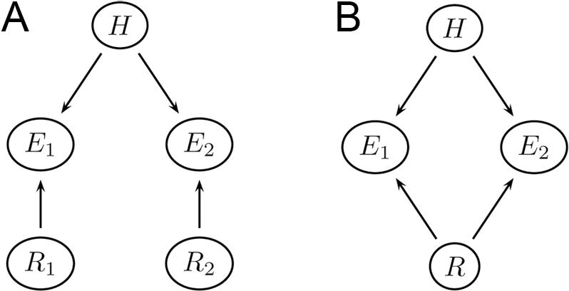
Two joint probability distributions are constructed over the set of variables . The assumed probabilistic independencies among the variables can be read off the Bayesian networks in figure 1 by using the d-separation criterion (Pearl Reference Pearl1988, 117–18).Footnote ⁵

Figure 1.

Two cases of partially reliable evidential sources. A, Independent reliability; B, shared reliability.

The probability distribution associated with the network in figure 1A is meant to capture the idea that two sources are reliability independent (i.e., ). The probability distribution associated with figure 1B captures the other extreme when evidential sources have fully shared reliabilities (i.e., ). The notion of variety modeled here is thus:

The joint probability distributions are further specified. The root variables H and R_i are given prior probabilities:

where h ₀ and ρ _i are parameters strictly between 0 and 1. The prior degree of belief that the hypothesis is true is thus , and ρ _i is the prior degree of belief that the evidential source i is reliable. For compactness, I will write for the prior probability that the hypothesis is false () and for the prior probability that source i is unreliable ().

What remains to be spelled out is how the evidential variable E_i varies with its parents. It is assumed that, when a source is reliable, the evidential report is a perfect truth tracker:

That is, when the hypothesis is true, a reliable evidential source will give a positive report; when the hypothesis is false, such a source will give a negative report.

What happens when the source is unreliable? To specify this case, Bovens and Hartmann rely on the following intuition:

This can be written

In other words, an unreliable source gives garbage information regarding the truth of the hypothesis. Upon learning the information from an unreliable source, the agent makes no updating to the subjective probability of the hypothesis.

Note that this is not the only plausible interpretation of ‘unreliable source’. The interpretation clashes, in particular, with the idea that unreliability might be due to calibration issues. Taking again the OPERA experiment as an example, some early critics claimed that the anomalous result might be due to a problem with clock synchronization (Contaldi Reference Contaldi2011). The estimated time of travel would be systematically below the actual time because the clock at the end of the tube clicked slightly later then the clock at the beginning.Footnote ⁶ With this type of unreliability, it is possible to undo the bias: given the estimated value and given the bias, one can retrieve the actual travel time. Knowing, for example, that the experimental setup is biased (¬r_i) in such a way that the estimated time is systematically underestimated by a factor b, obtaining a positive report e_i that the time of travel is t should matter for one’s belief in the hypothesis because an unbiased estimate of the travel time can be retrieved by computing . For such calibration problems, we thus have that , which contradicts condition (3). In this article, I stick to interpretations of unreliability compatible with condition (3) and keep the calibration interpretation for future work. I will later give examples of reasons for unreliability that are compatible with condition (3).

Condition (3) implies what follows (proof in Bovens and Hartmann Reference Bovens and Hartmann2003; app. C.1):

Another way to express this condition is .

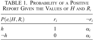
Parameter α _i is the last parameter of the model; it is the probability that the evidential report is positive, given that the source is unreliable. The probability that the evidential report is negative, given that the source is unreliable, is simply . Table 1 sums up how the realizations of E_i depend on the values taken by H and R_i.

Table 1.Probability of a Positive Report Given the Values of H and R_i

	ri	¬ri
h	1	α i
¬h	0	α i

Bovens and Hartmann offer a specific interpretation of α _i in terms of a randomizing evidential source. I will later offer an alternative interpretation of this parameter, but let me first reproduce their result relative to the variety-of-evidence thesis. The probability of interest is the posterior belief in the hypothesis given two positive reports: . For the two joint probability distributions and —that is, the distributions associated with the reliability-independent version (fig. 1A) and the shared-reliability version (fig. 1B)—this posterior can be written using the likelihood-ratio form

Which posterior is higher, or ? To turn this comparison into an assessment of the variety-of-evidence thesis, we need a plausible interpretation of the ceteris paribus condition of this thesis. Bovens and Hartmann impose restrictions that seem sufficient to meet the condition. First, we want to rule out comparing hypotheses starting with unequal degrees of confirmation. We thus impose . Second, we want the evidential sets to potentially differ in confirmatory strengths for no other reason than their relative variety. A sufficient condition for this goal is to require that all positive reports e_i in the independent-reliability and the shared-reliability versions have the same confirmatory strength for h—that is, for . This condition holds if the different α _i and ρ _i are reduced to only a single α and a single ρ across the two models (Bovens and Hartmann Reference Bovens and Hartmann2003, 104).

Given this interpretation of the ceteris paribus condition, the likelihood ratios associated with the two posteriors and are (proof in app. A)

Since we assume that the prior probability of the hypothesis is the same in the two models, the variety-of-evidence thesis implies that for all admissible parameter values—that is, we should have a higher confidence in the hypothesis if our two positive reports come from reliability-independent sources as compared to reliability-shared sources. This is equivalent to . It turns out, however, that the inequality is reversed for some combinations of values of α and ρ (proof in app. A):

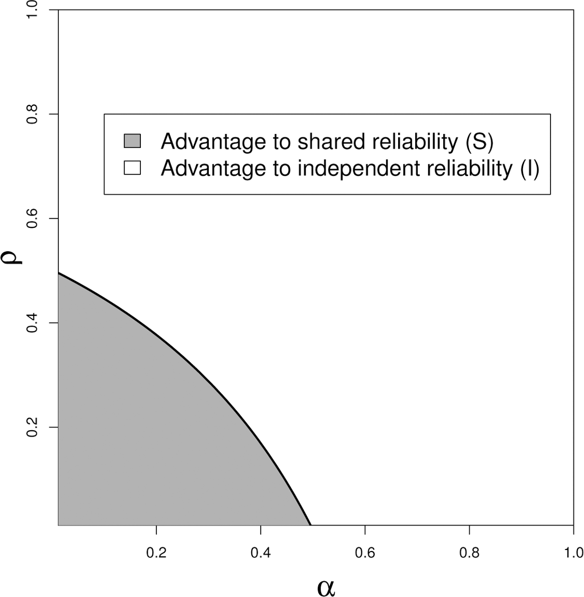
Figure 2 divides the parameter space in two regions: the bigger white region where independence is more confirmatory and the gray region where shared reliability is more confirmatory.

Figure 2.

Parameter space showing when shared reliability is more confirmatory than independent reliability.

What happens? Why is it sometimes better for confirmation to have no reliability independence rather than full independence? To understand this, it is crucial to see what shared reliability entails in the second version of the model, namely, that E ₁ is a truth teller if and only if E ₂ is a truth teller. As truth tellers, E ₁ and E ₂ will always give concordant reports. But when none of the evidential variables is a truth teller (i.e., when ¬r), then each evidential variable has a probability α of producing a positive report. It is crucial to recognize that this probability is not affected by the value the other evidential variable is realizing. It implies that when, and only when, they are unreliable, E ₁ and E ₂ might realize discordant reports. A second concordant report in the shared-reliability model thus contributes to confirmation in the following way: “we feel more confident that the instrument is not a randomizer and this increase in confidence in the reliability of the instrument benefits the confirmation of the hypothesis” (Bovens and Hartmann Reference Bovens and Hartmann2003, 98). The region of the parameter space where shared reliability is better is the one where this channel of ‘higher confirmation of h because higher confidence in the reliability of the source’ is the most effective. With low values of α, it is unlikely that an unreliable source would output two positive reports; it is thus likely that the two positive reports come from a reliable source. With low values of ρ, the agent starts with little confidence in the source; there is both great room for improving confidence and little to be gained for the belief in the hypothesis from the direct effect of a positive report since such a report is not likely to be truth tracking.

3. Questioning Bovens and Hartmann’s Result

While the logic of this result is simple, its implications for the variety-of-evidence thesis are less clear. As Bovens and Hartmann (Reference Bovens and Hartmann2003, 95n) recognize, the result of their model “does not apply to unreliable instruments that do not randomize.” It thus seems that the champions of the variety-of-evidence thesis would have little to worry about if evidential sources were rarely as Bovens and Hartmann depict them to be. And it indeed seems to be the case that scientists do not think of their evidential sources in the manner depicted by the shared-reliability model.

For example, consider the macrodata evidence for the hypothesis that one cause of the relatively high French unemployment rate is its relatively long duration of unemployment benefits. To simplify, let us imagine that the macrodata evidence is Pearson’s correlation coefficient between the legislated duration of unemployment benefits and the unemployment rate for a sample of industrial countries. There are many potential reasons why this coefficient would not be truth tracking (i.e., would be unreliable) with respect to the hypothesis of interest—for example, the correlation might not be a sign of causation from benefits to the unemployment rate because of the presence of a common cause, or perhaps the causal structure in France deviates substantially from the ones in the sampled countries.

Now imagine that I decide to compute the correlation coefficient twice. That is, I have the data for the two variables in my computer, and I use my favorite statistical software to compute the correlation twice (e.g., send the command cor(Bd,U) to R twice). It is reasonable to say that the two results would share a single reliability state: my second correlation coefficient would be reliable evidence for the hypothesis if and only if my first coefficient is also reliable evidence for the hypothesis. Does Bovens and Hartmann’s shared-reliability situation come anywhere close to capturing how we think about these two results? Obviously not.

According to the model, the two results will always be in concordance if the procedure is reliable. This implication seems fine. But something strange must happen with my statistical software when the procedure is unreliable. In this case, the two results might be at odds. Furthermore, if I were to compute the coefficient again and again, I would necessarily get discordant results (provided α is strictly between 0 and 1). To be sure, it is possible that my procedure is unreliable and is randomizing in this way. My correlation command might have been redefined such that it randomly outputs a number between −1 and 1. However, this is not what would normally be of concern. The reasons given above for why a correlation might be unreliable evidence for a specific causal claim will not bring about such randomness. If, for example, there is a confounding common cause, one would expect both coefficients to be identically affected.

Another way to see the problem with the model is to imagine that the data used to compute the correlation coefficients are known to be totally unrelated to French unemployment. Let us say that the two variables are the respective prices of two types of fish at the Grote Markt in Rotterdam. Since the correlation between these two variables is not tracking the truth of the hypothesis about French unemployment, the source is unreliable for this hypothesis (). Now the model tells us that, since the source is unreliable, the two computed correlations must be probabilistically independent. The agent thus starts with some strength of belief α that the correlation between the fish prices is positive. She sends the correlation command and reads a first positive coefficient. Strangely, learning this first coefficient will not make her revise her belief about the probable value of the second coefficient; just before pressing Enter again on her computer, she will still believe to strength α that the computer output will be positive.

The counterintuitiveness of Bovens and Hartmann’s model is not an artifact of my specific choice of example. Take the complex experimental setup of the OPERA Collaboration. Imagine that the research team—before announcing that it had located biases in its experimental procedure—had rerun the experiment with the exact same setup (imagine this to be the case even though the exact same setup is a physical impossibility) and that the results had corroborated the initial measurement. What would have been the reaction of the scientific community? The model tells us that the new results should have been taken as evidence that the setup is truth tracking. But it seems more intuitive that these results would have been met with indifference. Scientists distrusted the first measurement because they believed that the experiment suffered from a systematic (yet unknown) bias. Concordant results from a second identical experiment could thus be explained away by saying that the systematic bias was again operating (as it should if experimenters were careful enough in reproducing the setup). To make some progress in the debate, OPERA researchers needed to find a way to decrease the strength of the belief in the existence of a systematic bias. Rerunning the exact same experiment over and over would not have achieved that.

The upshot of this discussion is that the result of Bovens and Hartmann, as it stands, should not worry scientists and philosophers very much, if at all. There is still room for an unqualified variety-of-evidence thesis when the sources of evidence resemble the ones in science, rather than the ones in the model.Footnote ⁷

4. First Modification to the Model

Doubt has crept in: Can it not be shown that a more appropriate modeling of the evidential sources still results in a qualified variety-of-evidence thesis? In this section, I offer a negative answer to this question by making a single modification to the model of Bovens and Hartmann.

Bovens and Hartmann’s modeling choices are guided by a specific interpretation of the parameter α: for them it means that an unreliable evidential source acts like a randomizer. This becomes clear in their discussion of witnesses as a special case of an evidential source: “So, we assume that if witnesses are not reliable, then they are like randomizers. It is as if they do not even look at the state of the world to determine whether the hypothesis is true, but rather flip a coin or cast a die to determine whether they will provide a report to the effect that the hypothesis is true” (Bovens and Hartmann Reference Bovens and Hartmann2003, 57). While they interpret the parameter as capturing a property of the evidential source, I would rather interpret it from the point of view of the agent: just knowing that the source i is unreliable, α _i is the agent’s degree of belief that the report of this source will be positive.

It turns out that Bovens and Hartmann could have modeled this epistemic fact in a different way. Such an alternative way specifies that an unreliable evidential source is systematically biased, not randomizing. I want to emphasize at the outset that systematically biased sources of the kind I will model do not cover all the potential kinds of unreliability in science. Obviously, they do not cover randomizing sources (if such sources exist). More important, they fail to encompass the miscalibrated sources previously mentioned in section 2.

I still think that what I model as ‘systematically biased sources’ capture important reasons why one can judge a source to be unreliable. Here are a few hints at these reasons without any claim to be comprehensive. One general class of cases comprises the diverse ways in which an evidential report can be affected by a preconceived view of what is the ‘good’ answer. That might come from researchers performing data mining until they get the answer they want or from them simply falsifying their results because of their sponsor’s interests. It can also come from institutional pressures in science: peer review systematically favoring some sort of result or deeply rooted hypotheses making scientists revise their experimental procedure until the output fits ‘what is known’.

Another class of cases has to do with the risks of using something as a stand-in (as a model) in order to learn about something else. If one uses, for instance, an animal to learn about the potential side effects of a drug on humans, the extrapolation might go wrong because there is some biological mechanism in the model not present in the target (or the other way around), which makes the drug have some effect in one group of subjects but not in the other. The result from the model subjects will thus be systematically biased when used as a report for the target subjects.

To model sources that are potentially systematically biased, I redefine the reliability variable:

• • The new reliability variable , where r_i stands, as before, for the proposition that the source is reliable, stands for the proposition that the source is biased toward a positive report for the hypothesis regardless of its truth, and stands for the proposition that the source is biased toward a negative report.

This ternary variable (all the previous variables were binary) is arrived at by giving a more finely grained specification of the proposition ¬r_i. It is now decomposed into two disjoint propositions—that is, we now have .

My first modification inserts this new variable into the previous model. The probabilistic independencies that can be read off the Bayesian networks in figure 1 still hold. Furthermore, the specifications of the prior probabilities h ₀ and ρ _i in condition (1) are retained. We need, however, to specify more probabilities for R_i:

This condition assigns prior probabilities to the propositions about positive and negative biases given that the source is already known to be unreliable. Note that what was interpreted as a ‘randomization parameter’ by Bovens and Hartmann is used explicitly as a strength of belief here. Combining condition (9) with condition (1), we have what follows: the prior probability of a positive bias is , and the prior probability of a negative bias is .

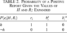
Finally, we need to expand table 1 by stating explicitly how likely e_i is, conditional on and . This expansion gives us table 2. Since the uncertainty that figured initially in has been shifted to R_i, the evidential variable E_i is now a deterministic function of H and R_i. This deterministic relation might come as a surprise to some, but it should not be surprising. If we remain committed to the irrelevance of an unreliable source (IUS), the columns for and for in table 2 must each contain the same value twice. If instead of having 1 and 0 for these values, we opt for values strictly between these two, we reintroduce into the model Bovens and Hartmann’s unreliability as randomizing. The counterexamples used in section 3 would thus apply. As long as we remain committed to the IUS condition, the notion of a systematic bias must be captured by a deterministic function. In future work, I will drop the IUS condition in the context of calibration issues, but I keep it here since it seems pertinent for some sources of unreliability.

Table 2.Probability of a Positive Report Given the Values of H and R_i: Expanded

	ri
h	1	1	0
¬h	0	1	0

The probabilities in table 2 and in equations (9) give us two new versions of the model. Define as the joint probability distribution associated with the independent-reliability situation (i.e., the distribution associated with fig. 1A) and as the distribution associated with the shared-reliability situation (i.e., the distribution associated with fig. 1B). We can now assess the variety-of-evidence thesis: Is it always the case that ?

In fact, is no different from —that is, for the case of sources with independent reliabilities, Bovens and Hartmann’s version and my version give the same result (proof in app. B). This is welcome news, given that Bovens and Hartmann’s version seems to capture what one means in saying that two evidential reports are fully independent regarding a hypothesis—that is, it concurs with what Shogenji (Reference Shogenji2005, 308) presents as “a general consensus among probability theorists on how to formalize the condition that two pieces of evidence E ₁ and E ₂ are independent of each other with respect to proposition A.”Footnote ⁸

Things are different when we turn to the new version with shared reliability. The posterior probability of the hypothesis is now (proof in app. B)

The likelihood ratio is identical to the one resulting from an evidential set with only a single element instead of two (see eq. [A5]). In other words, adding a second positive report in this new shared-reliability model has no effect on the degree of confirmation of the hypothesis. The reason for this result is simple: the second report cannot be anything but consistent with the first report in this model. The two evidential variables not only share reliability; they also share the direction of the bias if they are indeed biased. There is no longer the possibility of detecting that a source is unreliable by finding discordant reports coming from this source. Since this possibility no longer obtains, multiplying the reports from the same source becomes useless.

Is it still possible that the reports in the shared-reliability situation are more confirmatory than the ones in the independent-reliability situation? No. The posterior probability of h is strictly higher in the independency case if the probability that the sources are reliable is higher than 0 (see app. B for the proof). There is thus no combination of admissible parameter values for which having shared reliability is, ceteris paribus, better. Using the same source again is not conducive to confirmation because it no longer holds the promise of detecting the potential unreliability of the source. A second independent report is thus necessarily more confirmatory. The variety-of-evidence thesis holds without qualification in this version of the models.

5. Degrees of Independence

The result supporting the variety-of-evidence thesis in the previous section suffers from a major limitation. While the variety-of-evidence thesis explicitly compares more independent to less independent evidential elements, the comparison made with our two models is between fully independent and fully dependent evidential elements. Our comparison of confirmation was restricted to the two ends of a spectrum, whereas the variety-of-evidence thesis deals with how confirmation changes with changes in the degree of independence.

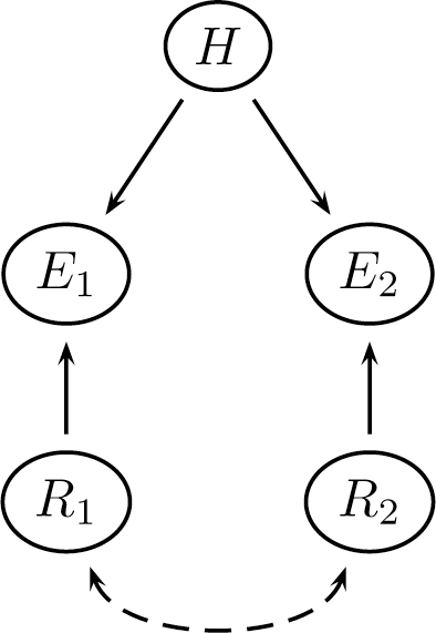
There is a simple way to model degrees of independence by extending the setup of the previous section. The graphical representation of this extended model is in figure 3, and its associated probability distribution will be labeled . The modification here adds a probabilistic association between the two reliability variables R ₁ and R ₂.Footnote ⁹ The rest of the model remains intact.

Figure 3.

Extended model with degrees of independence.

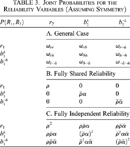
The association between the reliability variables is fully captured by specifying the probabilities for the nine possible combinations of their values. Panel A of table 3 offers a general notation for these nine possibilities. For instance, is the probability that both sources are reliable. The elements on the main diagonal () are the probabilities associated with the proposition that the two sources are in the same reliability state. Note that the table already assumes symmetry between the two sources—that is, , and so forth. This assumption was also used in the previous sections as part of the assumptions sufficient to meet the ceteris paribus condition of the variety-of-evidence thesis.

Table 3.Joint Probabilities for the Reliability Variables (Assuming Symmetry)

	r 2
	A. General Case
r 1	ω rr	ω rh	ω r¬h
	ω rh	ω hh	ω h¬h
	ω r¬h	ω h¬h	ω ¬h¬h
	B. Fully Shared Reliability
r 1	ρ	0	0
	0		0
	0	0
	C. Fully Independent Reliability
r 1	ρ 2

In this new model, the posterior belief in the hypothesis given two positive reports is (proof in app. C.1)

Table 3 panels B and C give the specific values taken by the ω’s for the two extreme cases on which the previous sections focused. It can be easily verified using these values that the expression in equation (11) reduces to equation (10) or (6) for each of these extreme cases—that is, the model of the previous section is fully embedded into this one (including its result for the variety-of-evidence thesis).

Is there a ready measure of degrees of independence? My proposal is based on the following consideration. Compare table 3 panels B and C. The probability mass is all on the main diagonal in the first case. In other words, it never happens that the two sources are in different reliability states. In the case of full independence, the probability mass is more spread out since the joint probability is simply the product of the marginal probabilities (i.e., ). In fact, each element on the main diagonal in table 3, panel C, is exactly the square of the same element in table 3, panel B. This fact suggests a specific metric to characterize degrees of independence.

Define a variable that is interpreted as measuring the distance of the evidential set from fully shared reliability—that is, when we have no independence, when we have full independence, and when δ is strictly between 0 and 1, we have only partial independence. Given values for ρ, α, and δ, the elements on the main diagonal are

These relations entail that the probability mass is shifted away from the elements on the main diagonal as the degree of independence increases. In other words, it becomes less likely that the two sources share the same reliability state.

With this variable δ, the variety-of-evidence thesis can be restated.

The restatement of the thesis is thus that the posterior degree of belief in the hypothesis invariably increases as we marginally increase the degree of independence of the evidential sources.

Before we assess this thesis, we need to specify how the off-diagonal elements in table 3, panel A, change as δ is modified. One obvious restriction is that the sum of all the elements (the nine ω’s) must be 1. The interpretation of the ceteris paribus condition previously used also restricts the values of the off-diagonal elements but not enough to ensure uniqueness. In addition to these restrictions, I thus also stipulate that the marginal probabilities of R ₁ and R ₂ are not a function of δ—that is, , , and , for and for all (see app. C.2).

This model leads to a qualification of the variety-of-evidence thesis (proof in app. C.3). Increasing the degree of independence leads to more confirmation if and only if the following condition holds:

But there are combinations of admissible values for ρ, α, and δ that violate this condition.

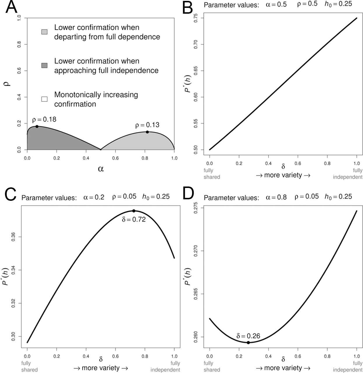
Figure 4 presents graphically the different possibilities. For most combinations of ρ and α, the relationship between degree of independence and confirmation is as stated by the variety-of-evidence thesis (fig. 4B presents such a case).Footnote ¹⁰ Figure 4A shows that there are in fact two distinct regions of the parameter space where the relationship between independence and confirmation is nonmonotonic. These two possibilities share (extremely) low values of ρ. In other words, these are situations in which prior information leads the agent to believe that it is highly unlikely that a given source is truth tracking. The relationship is indeed always monotonic when the trust in the source is above .18 (in Bovens and Hartmann’s model this was .5).

Figure 4.

Nonmonotonicity is possible. A, Parameter combinations resulting in a nonmontonic relationship between degrees of independence and confirmation; B, monotonic relationship; C, low α; D, high α.

There are two features distinguishing the two nonmonotonic situations from each other. First, as shown in figure 4A, they differ in their values for α—that is, the probability that the report is positive given that the source is unreliable. Second, as is evident by comparing figure 4C and 4D, the two regions are associated with different shapes of nonmonotonicity (concave vs. convex functions).

What is going on? As in Bovens and Hartmann’s model, what happens is that, upon learning e ₁ and e ₂, the agent reassesses the probability that the sources are reliable. The region of the space where confirmation decreases with independence is exactly the region where trust in the reliability of the sources decreases with independence (proof in app. C.4). In other words, to compare two evidential sets (for h)—say and , which differ only with respect to their degree of reliability independence (δ) (the elements of being more independent than the elements of )—one simply needs to assess the following ratio for each set:

The set with the higher ratio is more confirmatory than the other. The numerator of this ratio captures the probability of realizations of R ₁ and R ₂ that generate two evidential elements (e ₁ and e ₂) that are indeed truth revealing for h. The denominator is the probability that the two sources are producing positive-but-garbage reports for h. The denominator of will always be smaller than that of . This fact might capture the intuitive appeal of the variety-of-evidence thesis: it is less likely to get two garbage reports from sources that are (more) independent. But the full ratio is what ultimately decides between and .

Let me briefly discuss the only two situations in which the variety-of-evidence thesis is turned upside down. First, for low values of α combined with extremely low values of ρ (as in fig. 4C), getting two positive reports comes as a surprise—it was judged far more likely to receive at least one negative report because of the realization of . In this case, moving toward independence is initially beneficial, but more independence becomes detrimental to confirmation as one approaches the extreme of full independence. This result is interesting because it means that slightly departing from full independence sometimes increases confirmation.

Second, for high values of α combined with extremely low values for ρ (as in fig. 4D), getting two positive reports is not surprising; however, the agent judges it highly likely that the information is worthless (because and are likely to be realized). In this case, a departure from full dependence adversely affects confirmation. An implication of this nonmonotonicity is that the second positive report can be disconfirming h (i.e., ). Remember from section 4 that the posterior belief in h after two fully dependent reports (i.e., ) is identical to the posterior belief after a single report. Both are represented by the point at the extreme left of the curve in figure 4D. All the points lying below this point are thus cases in which the second report is disconfirming h. The agent puts so little trust in the evidential sources that a second report is interpreted as a sign that both sources are positively biased, and the initial (slight) increase in the belief for h is cut back.

6. Conclusion

The variety-of-evidence thesis seems to be a widespread implicit guideline in scientific practice. This thesis says that, ceteris paribus, the confirmatory power of an evidential set for a given hypothesis increases with the diversity (i.e., the independence) of the evidential elements in the set. Thus, one should praise ‘independent evidence’ and be suspicious of the rest.

Bovens and Hartmann (Reference Bovens and Hartmann2002, Reference Bovens and Hartmann2003) cast doubt on the universal applicability of this thesis by showing with a simple model that, in some peculiar epistemic situations, it is sometimes a disadvantage for confirmation to have independent evidential elements, ceteris paribus. I have argued that the relevance of this result is diminished by two characteristics of their model.

First, their idea that unreliable sources are randomizers leads them to model fully dependent sources in a way that is unlikely to reflect how scientists think about their sources of evidence. The problem is that Bovens and Hartmann assume that two fully dependent sources still produce two independent reports when they are unreliable (i.e., ). Instead, in actual scientific settings it seems to be the case that two reports coming from fully dependent sources will always coincide, even when the sources are unreliable. In section 4, I showed that the variety-of-evidence thesis is rehabilitated once the independent-randomizer assumption is dropped and replaced with the assumption that an unreliable source is systematically biased. This modification is compatible with the key intuition behind the notion of reliability in Bovens and Hartmann’s model (i.e., IUS).

Second, there is another serious limitation in Bovens and Hartmann’s model, a limitation that my first modification of their model shares. The comparison made to assess the variety-of-evidence thesis is between extremes; it is between fully independent and fully dependent evidential elements. The most relevant comparison is rather one of degree: less versus more independence of the sources. In section 5, I showed that when the model is modified to enable comparisons of degrees of independence, the variety-of-evidence thesis needs to be qualified. There are special epistemic situations wherein more independence does not give more confirmation. This qualification only applies to a subinterval of the spectrum from full dependence to full independence. Indeed, the two extremes of the spectrum always stand in the confirmatory relationship depicted by the variety-of-evidence thesis.

Where do my modeling efforts leave us? First, the usual caveat about idealization applies: it might well be that the way in which epistemic situations have been modeled here does not capture what is pertinent for the variety-of-evidence thesis. It is certain that my model does not encompass all the ways in which an evidential source can be unreliable (e.g., the calibration problems mentioned in sec. 2).

Even if one accepts the idealizations, the conclusion to draw about the variety-of-evidence thesis is not straightforward. One plausible reaction to the result of the last section is as follows. The variety-of-evidence thesis can break down in the extended model only if the agent has enormous doubts about the reliability of the evidential source; she must judge it to be at least 82% likely that the source is unreliable. One could thus read the result as highlighting the danger of using extremely weak evidential sources, rather than as a direct refutation of the variety-of-evidence thesis. This thesis could be interpreted as implicitly assuming that the evidential sources are sufficiently trustworthy to begin with. The fate of the variety-of-evidence thesis is not yet settled.