1 Introduction
Despite the prevalence of surfactants in confined biological and subsurface settings, their influence on fluid interfaces squeezing between solid boundaries remains largely uncharacterized. Surfactant-laden drop flow in the vicinity of solid obstacles gives rise to significant complexities due to the nonlinear coupling of interfacial hydrodynamics with surfactant transport and solid-phase contributions. A diverse set of fields including biomicrofluidics, solid-phase catalysis and enhanced oil recovery may benefit from theoretical insight into this commonly encountered but non-trivial system. Of fundamental interest is the ability to predict how the presence of surfactant affects drop transport through porous/granular media with respect to degree of contamination and fluid properties of the dispersed phase (Zinchenko & Davis Reference Zinchenko and Davis2017b ). To shed light on the influence of contamination on droplet flow near interstitial sites, a robust formulation for a surfactant-laden drop squeezing through a single interparticle constriction is developed in the present study.
There have been successful modelling efforts for each of the disparate components of the current system, namely (i) tight squeezing of clean drops and (ii) the effect of surfactant on fluid-phase emulsion flow without solid boundaries. Previous work has illuminated the critical role of lubrication forces between two approaching drops (Lee & Hodgson Reference Lee and Hodgson1968; Davis, Schonberg & Rallison Reference Davis, Schonberg and Rallison1989) or between a drop and a solid obstacle (Barnocky & Davis Reference Barnocky and Davis1989; Neitzel & Dell’Aversana Reference Neitzel and Dell’Aversana2002). These forces allow a drop to closely approach a substrate without wetting the surface. In experimental studies, this separation has been cited as reducing to the level of a monolayer or a few layers of water molecules (Chen et al. Reference Chen, Dong, Husein and Bryant2018). Numerical Stokes flow solutions using idealized spherical obstacles also predict that tightly squeezing drops nearly coat solid particles, with drop–solid clearances several orders of magnitude smaller than droplet radii (Zinchenko & Davis Reference Zinchenko and Davis2006). Therefore, modelling squeezing phenomena requires considerable robustness from numerical algorithms, which might be achieved with either interface capturing methods, such as that used by De Menech et al. (Reference De Menech, Garstecki, Jousse and Stone2008) for squeezing through microchannels, or desingularization techniques for formulations such as the boundary-integral method that specifically resolve the interface. A larger body of literature exists concerning the fundamental role of surfactants on fluid–fluid interfacial dynamics. One macroscale effect of surfactant is the reduction of surface tension. Contaminants also introduce an additional tangential stress along the interface due to gradients of surface tension, known as Marangoni stresses, which are responsible for interfacial stabilization or immobilization (Hosokawa et al. Reference Hosokawa, Masukura, Hayashi and Tomiyama2017). At high enough concentrations of certain surfactants, the surface can remobilize due to its inability to sustain the gradients necessary for Marangoni stresses (Stebe, Lin & Maldarelli Reference Stebe, Lin and Maldarelli1991).
Much of the conventional wisdom regarding contaminated-interface behaviour involves one or more drops in pure fluid. The surface diffusivity of a typical surfactant is extremely weak, on the order of
 $10^{-6}$
cm
 $^{2}$
s
 $^{-1}$
, and therefore much study has been devoted to non-diffusive surfactants (Eggleton, Pawar & Stebe Reference Eggleton, Pawar and Stebe1999). This assumption corresponds to the limit of large surface Péclet number
 $Pe\rightarrow \infty$
, typical of highly confined multiphase flows (Anna Reference Anna2016; Wrobel et al.
Reference Wrobel, Booty, Siegel and Wang2018). Here,
 $Pe=UL/D_{s}$
, where
 $U$
is a characteristic surface velocity (e.g. drop settling velocity or imposed interstitial flow velocity),
 $L$
is a characteristic length scale (e.g. drop diameter) and
 $D_{s}$
is surface diffusivity of surfactant. For example, using the above surface diffusivity, and a 1 mm droplet flowing through a packed bed with interstitial velocity
 $0.1~\text{cm}~\text{s}^{-1}$
, a conservative estimate (see e.g. Lebon et al.
Reference Lebon, Oger, Leblond, Hulin, Martys and Schwartz1996), gives
 $Pe\sim 10\,000$
. The model of non-diffusive surfactant continues to apply even for a drop trapped in a constriction, with near-zero advancement velocity. In this case, the correct velocity scale in the Péclet number definition is a much larger tangential interface velocity (due to internal circulation); this velocity can be on the order of the single-phase flow field (see § 5.2). In an imposed flow field such as extensional flow, surfactant tends to be swept in the direction of the flow and accumulate at drop poles. Surfactant localization can result in increased drop deformation, breakup or tip streaming, or a ‘stagnated cap’ as Marangoni stresses negate the developing surface stress field (Stone & Leal Reference Stone and Leal1990; Milliken, Stone & Leal Reference Milliken, Stone and Leal1993; Kruijt-Stegeman, van de Vosse & Meijer Reference Kruijt-Stegeman, van de Vosse and Meijer2004). These phenomena tend to be enabled or enhanced by low drop-to-medium viscosity ratios (Eggleton et al.
Reference Eggleton, Pawar and Stebe1999).
Surfactants also influence the interaction of two or more drops by affecting the formation and draining of the lubrication layer, as has been investigated with respect to colliding drops (Yeo et al. Reference Yeo, Matar, Perez de Ortiz and Hewitt2003). Surfactant was concluded to retard the drainage of the lubrication layer due to interface immobilization. Interestingly, the viscosity ratio has a negligible effect on drainage dynamics when the film is immobilized (Klaseboer et al. Reference Klaseboer, Chevaillier, Gourdon and Masbernat2000). Furthermore, it requires only a small amount of surfactant to achieve an immobilized interface (Allan, Charles & Mason Reference Allan, Charles and Mason1961; Lin & Slattery Reference Lin and Slattery1982). Surfactant may also increase the deformability of dimples formed in the near-contact region, though it is not immediately obvious if this effect would accelerate or prolong lubrication layer draining (Chesters & Bazhlekov Reference Chesters and Bazhlekov2000; Dai & Leal Reference Dai and Leal2008).
The inclusion of a spatially fixed solid phase within a contaminated emulsion introduces a number of challenges, both in terms of physical modelling and accurate numerical treatment. Under tight-squeezing conditions, a droplet may approach the solid surface to within a distance several orders of magnitude less than the radius of the droplet (Bordoloi & Longmire Reference Bordoloi and Longmire2014). In the context of a boundary-integral formulation, this proximity necessitates higher-order desingularization techniques customized for the solid-phase contribution that account for both hydrodynamic (normal) and Marangoni (tangential) forces acting on the interface. Additionally, unlike isolated drops settling under gravity or subject to simple flows, complex patterns of surfactant may develop on the drop surface and be maintained at steady state, including the appearance of sharp concentration gradients. With respect to a numerical implementation, it was found in the present work that a stable algorithm for surfactant convection, particularly at low drop-to-medium viscosity ratios and negligible diffusion, requires the use of an upwind-biased scheme. Finally, it is not immediately obvious how lubrication forces between a solid particle and a deformable drop will be affected after contaminating the drop. The coupling between these physical considerations make it difficult to intuit the extent to which surfactant should increase or decrease squeezing times, assumed to be dependent on the competing effects of locally increased surface deformability and immobilization of the drop interface. Therefore, a fully three-dimensional model that explicitly resolves the interface is necessary for investigating contaminated-drop squeezing.
The technical aspect of modelling surfactant contributions largely revolves around accurately capturing interface phenomena and has been achieved with space-filling gridded techniques, such as front-tracking (de Jesus et al. Reference de Jesus, Roma, Pivello, Villar and da Silveira-Neto2015), embedded-boundary (Khatri & Tornberg Reference Khatri and Tornberg2014), level-set (Xu, Yang & Lowengrub Reference Xu, Yang and Lowengrub2012) or phase-field (Liu & Zhang Reference Liu and Zhang2010) and lattice Boltzmann (Riaud et al. Reference Riaud, Zhang, Wang, Wang and Luo2018) methods. These efforts have primarily focused on drops subject to an imposed shear, extensional or channel flow. For example, Park, Hulsen & Anderson (Reference Park, Hulsen and Anderson2013) discussed the effect of surfactant on droplet formation through a flow-focusing device using a diffuse-interface method, suggesting that the drop radii decrease with increasing surfactant coverage. Riaud et al. (Reference Riaud, Zhang, Wang, Wang and Luo2018) elucidated the conditions under which stagnant caps can form on drops flowing through a T-junction microchannel, and that surfactant can reduce drop squeezing time in this situation. Farhat et al. (Reference Farhat, Celiker, Singh and Lee2011) showed that droplet elongation increases with surfactant coverage in simple shear and extensional flows, using a lattice Boltzmann approach. Using a similar method, Liu & Zhang (Reference Liu and Zhang2010) demonstrated that surfactants inhibit coalescence by reducing interface mobility and slowing film drainage. Finally, boundary-integral methods can be used to selectively solve for interfacial behaviour with respect to various equations of state (Li & Pozrikidis Reference Li and Pozrikidis1997; Eggleton et al. Reference Eggleton, Pawar and Stebe1999) as well as large degrees of drop deformation and breakup (Bazhlekov, Anderson & Meijer Reference Bazhlekov, Anderson and Meijer2006), using schemes of arbitrary order of accuracy.
Extending the goals of prior work by Zinchenko & Davis (Reference Zinchenko and Davis2006) on clean drops, we study herein how the surface contamination of a drop with insoluble surfactant affects its flow-induced squeezing through a constriction between several solid particles in the Stokes regime. To effect tight-squeezing conditions, the non-deformed drop diameter is larger than the constriction diameter. An immediate goal is to probe the effects of the surfactant surface coverage, capillary number and viscosity ratio on the squeezing time, surfactant distribution and critical conditions for drop trapping. Even more important for the research community, this small-scale but still challenging three-dimensional (3D) problem serves as a prototype for drop squeezing through a granular medium (with relevance e.g. to oil recovery). Robust simulation tools developed herein for surfactant transport will be indispensable in future multipole-accelerated, multidrop–multiparticle simulations for emulsion flow through a packed bed; as an example, boundary-integral desingularization tools from Zinchenko & Davis (Reference Zinchenko and Davis2006) were essential in large-scale simulations of Zinchenko & Davis (Reference Zinchenko and Davis2013) for clean drops.
The problem formulation, relevant parameters and simulation set-up are discussed in § 2. An overview of the boundary-integral equations is provided in § 3. Comprehensive analysis of various schemes for transport of non-diffusive surfactant on a deformable surface is given in § 4. The finite-volume algorithm (Bazhlekov, Anderson & Meijer Reference Bazhlekov, Anderson and Meijer2003) used for a single drop in shear flow, and the least-squares method of Zinchenko & Davis (Reference Zinchenko and Davis2017a ) for concentrated emulsions, turn out to be very restrictive in tight-squeezing simulations, not allowing, in particular, for small viscosity ratios. The difficulties with both methods (namely, surface tension becoming negative) in the zero-diffusion limit were puzzling and unresolved in prior work; physical deficiency of the linear equation of state for surfactant was even suspected (Bazhlekov et al. Reference Bazhlekov, Anderson and Meijer2006; Zinchenko & Davis Reference Zinchenko and Davis2017a ). We show here instead that the issue of negative surface tension arises from numerical instability and is eliminated by a flow-biased surfactant transport scheme. Two competitive stable schemes are offered in § 4, namely, an upwind finite-volume version for a deformable surface (more in line with traditional upwind algorithms in inviscid flow modelling, e.g. Smolarkiewicz & Szmelter (Reference Smolarkiewicz and Szmelter2005)), and a substantially new flow-biased least-squares method. Close agreement between the results by these two, very distinct, methods is the evidence that numerical diffusion (inherent in both methods) does not come into play appreciably in the range of parameters and resolutions of the present study. Convergent tight-squeezing simulations always require extreme resolutions anyway, both for drop and solid surfaces, even with the present boundary-integral algorithm that explicitly resolves the boundaries. So, it seems problematic to reach similar goals with alternative approaches using space-filling grids (e.g. with the volume of fluid (VOF) method). In §§ 5–6, we summarize major trends observed for contaminated-drop squeezing, with particular focus on the influence of surfactant on critical capillary number and interfacial behaviour under a wide range of viscosity ratios.
2 Problem formulation
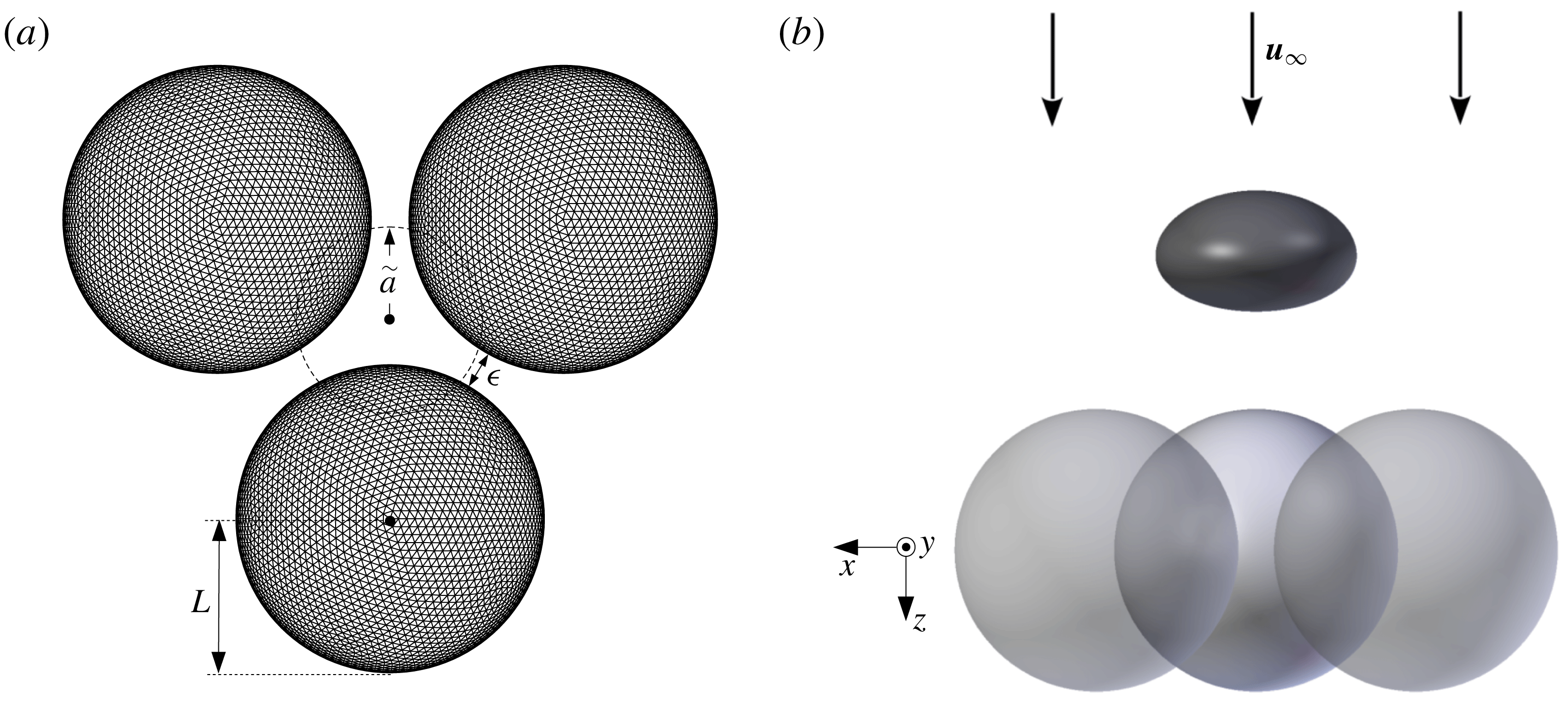
Consider a single deformable drop freely suspended in a uniform far-field flow, covered with an initially uniform insoluble surfactant and approaching an array of spatially fixed solid particles, where both liquid phases are described by Stokes flow and assumed Newtonian. A constriction is formed by three equi-sized solid spheres arranged in an equilateral triangle (as in figure 1
a, for a resolution of
 $N_{\triangle }=8640$
mesh triangles per particle). In what follows,
 $\widehat{N}_{\triangle }$
and
 $\widetilde{N}_{\triangle }$
will refer to solid-particle and drop mesh resolutions, respectively, and the abbreviations 8.6 K, 11.5 K, 15.4 K, 20 K and 46 K will be used for
 $N_{\triangle }=8640$
, 11 520, 15 360, 20 480 and 46 080. Defining the characteristic length
 $L$
of the system as the radius of a solid particle, the drop centre is initially placed
 $6L$
upstream of the particles’ basal plane, unless otherwise noted. The ratio between undeformed drop and solid radii,
 $\widetilde{a}/L$
, is fixed at 0.6, and the interparticle gap (
 $\unicode[STIX]{x1D716}$
) is fixed at 0.25
 $L$
, for all simulations herein. The ratio of the drop viscosity (
 $\unicode[STIX]{x1D707}_{d}$
) and medium viscosity (
 $\unicode[STIX]{x1D707}_{e}$
) is
 $\unicode[STIX]{x1D706}=\unicode[STIX]{x1D707}_{d}/\unicode[STIX]{x1D707}_{e}$
, and the uniform far-field velocity carrying the drop towards the constriction is
 $\boldsymbol{u}_{\infty }$
(figure 1
b).
Surfactant-concentration (
 $\unicode[STIX]{x1D6E4}$
, in moles/area) and surface-tension (
 $\unicode[STIX]{x1D70E}$
) gradients develop from their uniform distribution on the drop as it nears the constriction. An important metric of drop squeezing behaviour is the drop squeezing time
 $T_{s}$
. For the purposes of this study, a drop is defined to be in a squeezing state if its instantaneous centre-of-mass velocity
 $U$
(see below) is less than 1 % of the uniform far-field velocity
 $|\boldsymbol{u}_{\infty }|$
.
The non-dimensional elasticity parameter
 $\unicode[STIX]{x1D6FD}$
, a measure of the degree of surface contamination, is defined as
 $$\begin{eqnarray}\unicode[STIX]{x1D6FD}=\unicode[STIX]{x1D6E4}_{eq}\frac{RT}{\unicode[STIX]{x1D70E}_{o}}=\frac{Q}{4\unicode[STIX]{x03C0}\widetilde{a}^{2}}\frac{RT}{\unicode[STIX]{x1D70E}_{o}},\quad \text{where }Q=\int _{\widetilde{S}}\unicode[STIX]{x1D6E4}\,\text{d}S,\end{eqnarray}$$
 $\unicode[STIX]{x1D70E}_{o}$
signifies clean-drop surface tension,
 $\widetilde{S}$
represents the drop surface and equilibrium (
 $eq$
) is defined as the case of uniform surfactant concentration on a spherical drop. We assume a linear equation of state
 $\unicode[STIX]{x1D70E}=\unicode[STIX]{x1D70E}_{o}-RT\unicode[STIX]{x1D6E4}$
, where
 $R$
is the universal gas constant and
 $T$
the uniform absolute temperature. The equilibrium surface tension can then be expressed as
 $$\begin{eqnarray}\unicode[STIX]{x1D70E}_{eq}=\unicode[STIX]{x1D70E}_{o}(1-\unicode[STIX]{x1D6FD}).\end{eqnarray}$$
The capillary number is defined using the equilibrium surface tension:
 $$\begin{eqnarray}Ca=\frac{\unicode[STIX]{x1D707}_{e}|\boldsymbol{u}_{\infty }|}{\unicode[STIX]{x1D70E}_{eq}}\frac{\widetilde{a}}{L}.\end{eqnarray}$$
Several other metrics are used to quantify squeezing behaviour. The gap between the drop and each solid particle is defined as the minimum distance between the drop mesh polyhedron, assuming flat triangulation, and the particle centre minus the particle radius. The instantaneous drop velocity
 $\boldsymbol{U}$
, defined as the volume-averaged fluid velocity
 $\boldsymbol{u}$
inside the drop, can be calculated through the divergence theorem as
 $$\begin{eqnarray}\boldsymbol{U}=\langle \boldsymbol{u}\rangle =\frac{1}{\widetilde{V}}\int _{\widetilde{S}}(\boldsymbol{u}\boldsymbol{\cdot }\boldsymbol{n})(\boldsymbol{x}-\widetilde{\boldsymbol{x}}^{c})\,\text{d}S,\end{eqnarray}$$
where
 $\widetilde{V}$
is the drop volume,
 $\boldsymbol{n}$
are outward surface unit normals at points
 $\boldsymbol{x}$
on the surface and
 $\widetilde{\boldsymbol{x}}^{c}$
is the drop centroid. In what follows,
 $U$
is the component of
 $\boldsymbol{U}$
along
 $\boldsymbol{u}_{\infty }$
.
The simplest equation of state
 $\unicode[STIX]{x1D70E}=\unicode[STIX]{x1D70E}_{o}-RT\unicode[STIX]{x1D6E4}$
used herein (and elsewhere) is the linearization of the Langmuir–Szyszkowski equation
 $\unicode[STIX]{x1D70E}=\unicode[STIX]{x1D70E}_{o}+RT\unicode[STIX]{x1D6E4}_{\infty }\ln (1-\unicode[STIX]{x1D6E4}/\unicode[STIX]{x1D6E4}_{\infty })$
for
 $\unicode[STIX]{x1D6E4}\ll \unicode[STIX]{x1D6E4}_{\infty }$
, where
 $\unicode[STIX]{x1D6E4}_{\infty }$
is the maximum surfactant concentration for complete surface coverage as a monolayer; accordingly,
 $\unicode[STIX]{x1D6E4}_{\infty }$
falls out from the formulation. In our simulations, the surface average
 $\langle \unicode[STIX]{x1D6E4}\rangle$
remains close to
 $\unicode[STIX]{x1D6E4}_{eq}$
, due to surfactant conservation and modest changes in the drop surface area, even for significant deformations. For this reason,
 $\unicode[STIX]{x1D6E4}_{eq}\ll \unicode[STIX]{x1D6E4}_{\infty }$
(rather than
 $\unicode[STIX]{x1D6E4}\ll \unicode[STIX]{x1D6E4}_{\infty }$
) is believed to be an appropriate condition for linearization of
 $\unicode[STIX]{x1D70E}(\unicode[STIX]{x1D6E4})$
to not appreciably affect the global squeezing dynamics; incidentally, in our stable simulations with linear
 $\unicode[STIX]{x1D70E}(\unicode[STIX]{x1D6E4})$
, Marangoni stresses do not allow
 $\unicode[STIX]{x1D6E4}$
to greatly exceed
 $\unicode[STIX]{x1D6E4}_{eq}$
(thus keeping
 $\unicode[STIX]{x1D70E}$
positive). The condition
 $\unicode[STIX]{x1D6E4}_{eq}\ll \unicode[STIX]{x1D6E4}_{\infty }$
translates into
 $\unicode[STIX]{x1D6FD}\ll E$
, with
 $E=RT\unicode[STIX]{x1D6E4}_{\infty }/\unicode[STIX]{x1D70E}_{o}$
. From experimental data for several surfactants, Eggleton et al. (Reference Eggleton, Pawar and Stebe1999) report the values of
 $E\sim 0.15$
–
 $0.5$
, although there are no theoretical arguments why they cannot be higher. For
 $E\sim 0.3$
–
 $0.5$
, the condition
 $\unicode[STIX]{x1D6FD}\ll E$
is roughly met for most of our simulations.
Initial configuration for drop squeezing simulations. (a) Solid particles with meshing and undeformed droplet represented with a dashed circle. (b) Droplet in a uniform far-field flow deforms in the compressional-type flow upstream from fixed solid particles (rendered translucent).

3 Desingularized boundary-integral formulation
The present boundary-integral formulation for contaminated-drop squeezing combines the approaches previously developed for interparticle squeezing of clean drops (Zinchenko & Davis Reference Zinchenko and Davis2006) and free-space flows of contaminated emulsions (Zinchenko & Davis Reference Zinchenko and Davis2017a ). The Hebeker representation for solid-particle contributions is used along with custom, high-order desingularization techniques for drop–solid, solid–solid and self-interactions, in order to treat tight-squeezing conditions. The appearance of Marangoni stresses due to surfactant gradients results in an additional tangential component of the stress jump at the drop interface. The components of the interfacial stress are individually desingularized for both drop self-interactions and drop–solid contributions. The formulation results in well-behaved Fredholm integral equations of the second kind and allows accurate modelling of near-critical conditions, for which drop–solid separation distances can be several orders of magnitude smaller than the drop radius.
Let
 $\widetilde{N}$
be, for generality, the number of drops in the system,
 $\widetilde{S}$
be the surfaces of these drops,
 $\widehat{N}$
be the number of solid particles and
 $\widehat{S}$
be the surfaces of these particles. The no-slip boundary condition
 $\boldsymbol{u}=\mathbf{0}$
is enforced for the fluid velocity on the solid boundaries. The far-field velocity
 $\boldsymbol{u}_{\infty }(\boldsymbol{y})$
away from the particles and drops can be an arbitrary Stokes flow (although a uniform
 $\boldsymbol{u}_{\infty }$
was assumed in the present simulations). Standard Wielandt’s deflation is used to avoid ill-conditioning at the low viscosity ratios of interest for this study. To this end, the system is cast in terms of
 $\boldsymbol{w}=\boldsymbol{u}-\unicode[STIX]{x1D705}\boldsymbol{u}^{\prime }$
, where
 $\unicode[STIX]{x1D705}=(\unicode[STIX]{x1D706}-1)/(\unicode[STIX]{x1D706}+1)$
and
 $\boldsymbol{u}^{\prime }$
is the rigid-body projection of
 $\boldsymbol{u}$
. At every time step, the following system of equations is solved for modified interface velocity
 $\boldsymbol{w}$
on drops and Hebeker density
 $\boldsymbol{q}$
on solid surfaces:
 $$\begin{eqnarray}\displaystyle \boldsymbol{w}(\boldsymbol{y}) & = & \displaystyle \frac{2\boldsymbol{F}(\boldsymbol{y})}{\unicode[STIX]{x1D706}+1}+\unicode[STIX]{x1D705}\left[2\mathop{\sum }_{\unicode[STIX]{x1D6FD}=1}^{\widetilde{N}}\int _{\widetilde{S}_{\unicode[STIX]{x1D6FD}}}\boldsymbol{w}(\boldsymbol{x})\boldsymbol{\cdot }\unicode[STIX]{x1D70F}(\boldsymbol{r})\boldsymbol{\cdot }\boldsymbol{n}(\boldsymbol{x})\,\text{d}S_{x}-\boldsymbol{w}^{\prime }(\boldsymbol{y})+\frac{\boldsymbol{n}(\boldsymbol{y})}{\widetilde{S}_{\unicode[STIX]{x1D6FC}}}\int _{\widetilde{S}_{\unicode[STIX]{x1D6FC}}}\boldsymbol{w}\boldsymbol{\cdot }\boldsymbol{n}\,\text{d}S\right]\nonumber\\ \displaystyle & & \displaystyle +\,\frac{2}{\unicode[STIX]{x1D706}+1}\mathop{\sum }_{\unicode[STIX]{x1D6FD}=1}^{\widehat{N}}\int _{\widehat{S}_{\unicode[STIX]{x1D6FD}}}\boldsymbol{q}(\boldsymbol{x})\boldsymbol{\cdot }[2\unicode[STIX]{x1D749}(\boldsymbol{r})\boldsymbol{\cdot }\boldsymbol{n}(\boldsymbol{x})+\unicode[STIX]{x1D702}\unicode[STIX]{x1D642}(\boldsymbol{r})]\,\text{d}S_{x}\end{eqnarray}$$
for
 $\boldsymbol{y}\in \widetilde{S}_{\unicode[STIX]{x1D6FC}}$
and
 $$\begin{eqnarray}\displaystyle \boldsymbol{q}(\boldsymbol{y}) & = & \displaystyle \boldsymbol{F}(\boldsymbol{y})+(\unicode[STIX]{x1D706}-1)\mathop{\sum }_{\unicode[STIX]{x1D6FD}=1}^{\widetilde{N}}\int _{\widetilde{S}_{\unicode[STIX]{x1D6FD}}}\boldsymbol{w}(\boldsymbol{x})\boldsymbol{\cdot }\unicode[STIX]{x1D749}(\boldsymbol{r})\boldsymbol{\cdot }\boldsymbol{n}(\boldsymbol{x})\,\text{d}S_{x}\nonumber\\ \displaystyle & & \displaystyle +\,\mathop{\sum }_{\unicode[STIX]{x1D6FD}=1}^{\widehat{N}}\int _{\widehat{S}_{\unicode[STIX]{x1D6FD}}}\boldsymbol{q}(\boldsymbol{x})\boldsymbol{\cdot }[2\unicode[STIX]{x1D749}(\boldsymbol{r})\boldsymbol{\cdot }\boldsymbol{n}(\boldsymbol{x})+\unicode[STIX]{x1D702}\unicode[STIX]{x1D642}(\boldsymbol{r})]\,\text{d}S_{x}\end{eqnarray}$$
on solid-particle surfaces (
 $\boldsymbol{y}\in \widehat{S}_{\unicode[STIX]{x1D6FC}}$
), where
 $\boldsymbol{r}=\boldsymbol{x}-\boldsymbol{y}$
,
 $\boldsymbol{n}$
is the unit normal to the surface,
 $\unicode[STIX]{x1D702}>0$
is the Hebeker parameter (the choice of
 $\unicode[STIX]{x1D702}$
affects the algorithm robustness but not the solution upon numerical convergence) and a prime indicates rigid-body projection. The single-layer terms containing the Hebeker parameter
 $\unicode[STIX]{x1D702}$
serve to complete the range of boundary-integral operators; without these terms, the double-layer boundary-integral contribution could not accommodate non-zero forces or torques acting on the solid particles. Here, and for the remainder of § 3, the index
 $\unicode[STIX]{x1D6FD}$
should not be confused with the elasticity parameter. To account for Marangoni stresses, the boundary-integral equations are modified from Zinchenko & Davis (Reference Zinchenko and Davis2006) in the definition of
 $\boldsymbol{F}(\boldsymbol{y})$
, as
 $$\begin{eqnarray}\boldsymbol{F}(\boldsymbol{y})=\boldsymbol{u}_{\infty }(\boldsymbol{y})+\mathop{\sum }_{\unicode[STIX]{x1D6FD}=1}^{\widetilde{N}}\int _{\widetilde{S}_{\unicode[STIX]{x1D6FD}}}\boldsymbol{f}(\boldsymbol{x})\boldsymbol{\cdot }\unicode[STIX]{x1D642}(\boldsymbol{x}-\boldsymbol{y})\,\text{d}S_{x},\end{eqnarray}$$
with
 $$\begin{eqnarray}\boldsymbol{f}(\boldsymbol{x})=\frac{1}{\unicode[STIX]{x1D707}_{e}}(2\unicode[STIX]{x1D70E}(\boldsymbol{x})k(\boldsymbol{x})\boldsymbol{n}(\boldsymbol{x})-\unicode[STIX]{x1D735}_{s}\unicode[STIX]{x1D70E})\quad (\boldsymbol{x}\in \widetilde{S}_{\unicode[STIX]{x1D6FD}}),\end{eqnarray}$$
where
 $\unicode[STIX]{x1D735}_{s}$
is the surface gradient and
 $k$
is the mean surface curvature
 $k(\boldsymbol{x})=(k_{1}+k_{2})/2$
, with
 $k_{1}$
,
 $k_{2}$
being the principal curvatures at
 $\boldsymbol{x}$
. Finally,
 $\unicode[STIX]{x1D642}(\boldsymbol{r})$
and
 $\unicode[STIX]{x1D749}(\boldsymbol{r})$
are the free-space Green tensor and the corresponding fundamental stresslet, respectively:
 $$\begin{eqnarray}\unicode[STIX]{x1D642}(\boldsymbol{r})=-\frac{1}{8\unicode[STIX]{x03C0}}\left[\frac{\boldsymbol{I}}{r}+\frac{\boldsymbol{r}\boldsymbol{r}}{r^{3}}\right],\quad \unicode[STIX]{x1D749}(\boldsymbol{r})=\frac{3}{4\unicode[STIX]{x03C0}}\frac{\boldsymbol{r}\boldsymbol{r}\boldsymbol{r}}{r^{5}}.\end{eqnarray}$$
After desingularization of droplet–droplet, droplet–particle and particle–particle interactions, equations (3.1)–(3.2) can be solved by GMRES iterations, and node positions can be time-integrated using a second- or first-order Runge–Kutta scheme. An improved surface integration scheme, which treats the mesh triangles on spherical solid particles as curved geodesic triangles, allows for better convergence with respect to surface triangulation in drop squeezing simulations (see Zinchenko & Davis Reference Zinchenko and Davis2013). Mesh quality is maintained using passive mesh stabilization, as in Zinchenko & Davis (Reference Zinchenko and Davis2006).
Single-layer desingularization in (3.3) for an arbitrary vector field
 $\boldsymbol{f}(\boldsymbol{x})=\boldsymbol{f}_{\Vert }(\boldsymbol{x})+f_{n}(\boldsymbol{x})\boldsymbol{n}(\boldsymbol{x})$
, where
 $\boldsymbol{f}_{\Vert }$
is the tangential component and
 $f_{n}=\boldsymbol{f}\boldsymbol{\cdot }\boldsymbol{n}$
is the normal component, is achieved with the general relation
 $$\begin{eqnarray}\displaystyle \int _{S}\boldsymbol{f}(\boldsymbol{x})\boldsymbol{\cdot }\unicode[STIX]{x1D642}(\boldsymbol{x}-\boldsymbol{y})\,\text{d}S_{x} & = & \displaystyle \int _{S}[\boldsymbol{f}-(\boldsymbol{n}\boldsymbol{\cdot }\boldsymbol{n}^{\ast })\boldsymbol{f}_{\Vert }^{\ast }-(\boldsymbol{f}_{\Vert }^{\ast }\boldsymbol{\cdot }\boldsymbol{n})\boldsymbol{n}^{\ast }-f_{n}^{\ast }\boldsymbol{n}]\boldsymbol{\cdot }\unicode[STIX]{x1D642}(\boldsymbol{x}-\boldsymbol{y})\,\text{d}S_{x}\nonumber\\ \displaystyle & & \displaystyle +\,\int _{S}[(\boldsymbol{x}-\boldsymbol{x}^{\ast })\boldsymbol{\cdot }\boldsymbol{n}^{\ast }]\,\boldsymbol{f}_{\Vert }^{\ast }\boldsymbol{\cdot }\unicode[STIX]{x1D749}(\boldsymbol{x}-\boldsymbol{y})\boldsymbol{\cdot }\boldsymbol{n}\,\text{d}S_{x}.\end{eqnarray}$$
Here,
 $\boldsymbol{y}$
may be an observation point either on or outside
 $S$
. If
 $\boldsymbol{y}\in S$
then
 $\boldsymbol{x}^{\ast }=\boldsymbol{y}$
, otherwise
 $\boldsymbol{x}^{\ast }\in S$
is chosen as the mesh node on
 $S$
nearest to
 $\boldsymbol{y}$
. The superscript
 $^{\ast }$
denotes values at
 $\boldsymbol{x}^{\ast }$
, and
 $\boldsymbol{f}=\boldsymbol{f}(\boldsymbol{x})$
and
 $\boldsymbol{n}=\boldsymbol{n}(\boldsymbol{x})$
on the right-hand side for conciseness. Further technical details regarding these techniques have been discussed at length by Zinchenko & Davis (Reference Zinchenko and Davis2006, Reference Zinchenko and Davis2017a
).
4 Surfactant transport and numerical considerations
Surface diffusion of a typical surfactant is weak, and transport is dominated by surface convection in many cases of practical interest (see § 1). When neglecting diffusion, the transport of local surfactant concentration is solely due to convection and Marangoni stresses on the deformable drop surface. The problem therefore reduces to the pure convection of a non-negative scalar field confined to a closed, deformable surface. For tight-squeezing contaminated drops, a characteristic aspect of the surfactant distribution is the development of sharp concentration gradients, due to the interaction between Marangoni stresses and squeezing drop hydrodynamics. Several formulations were implemented in the present work in an attempt to achieve universal stability while adequately resolving these gradients. Simulations at high viscosity ratio (
 $\unicode[STIX]{x1D706}=4$
) were completed using the least-squares scheme with small, variable artificial diffusion (with the goal of achieving the zero-diffusion limit globally) presented in detail by Zinchenko & Davis (Reference Zinchenko and Davis2017a
), but this method was found to develop numerical instabilities at low drop-to-medium viscosity ratios. An alternative discussed therein, namely utilizing a simple conservation law for purely non-diffusive surfactant, was also tested extensively but simulations crashed at similar times, due to numerical oscillations resulting in local areas of unphysically high surfactant concentrations. The non-diffusive, finite-volume formulation for unstructured surface meshes presented by Bazhlekov et al. (Reference Bazhlekov, Anderson and Meijer2003) was explored in the present work with options for explicit, semi-implicit and implicit time integration, and was found to significantly increase stability but was unable to continue simulations to drop exit, also due to oscillatory behaviour at low viscosity ratios. Instead, a first-order upwind finite-volume scheme was found to stably model surfactant transport while still resolving the surfactant distribution without diffusion. Finally, a stable flow-biased least-squares scheme (without diffusion) was developed, which also decreases the order of surfactant-gradient fitting but retains higher-order velocity fitting for each node. Results as well as convergence behaviour obtained using this latest scheme were found to agree with those by the upwind finite-volume scheme.
A consideration common to all implementations is accounting for nodal velocity
 $\boldsymbol{V}=\boldsymbol{u}+\boldsymbol{w}$
not being equal to interfacial velocity
 $\boldsymbol{u}$
, due to the use of passive mesh stabilization to maintain mesh quality. We begin with the dimensional convection–diffusion equation for a deformable surface,
 $$\begin{eqnarray}\frac{\text{d}\unicode[STIX]{x1D6E4}}{\text{d}t}=\boldsymbol{w}\boldsymbol{\cdot }\unicode[STIX]{x1D735}_{s}\unicode[STIX]{x1D6E4}-\unicode[STIX]{x1D6E4}\unicode[STIX]{x1D735}_{s}\boldsymbol{\cdot }\boldsymbol{u}-2k\unicode[STIX]{x1D6E4}\boldsymbol{u}\boldsymbol{\cdot }\boldsymbol{n}+D_{s}\unicode[STIX]{x1D6FB}_{s}^{2}\unicode[STIX]{x1D6E4},\end{eqnarray}$$
where
 $\text{d}/\text{d}t$
is the time derivative for a node moving with velocity
 $\boldsymbol{V}$
,
 $\boldsymbol{u}$
is the interfacial fluid velocity,
 $k$
is the local mean curvature,
 $\boldsymbol{n}$
is the drop surface outward normal,
 $D_{s}$
is the surfactant diffusivity (set to zero when neglected, see below), and
 $\unicode[STIX]{x1D735}_{s}$
is the surface gradient operator (by definition, only the tangential component
 $\boldsymbol{u}_{s}$
of
 $\boldsymbol{u}$
participates in the divergence operation
 $\unicode[STIX]{x1D735}_{s}\boldsymbol{\cdot }\boldsymbol{u}$
). Also, in all implementations, surfactant concentration is rescaled at every time step to preserve the total amount of surfactant over long simulation times (even though, at each time step, the rescaling factor is extremely close to unity and approaches this limit for high resolutions).
4.1 Least-squares scheme
The least-squares (LS) scheme detailed in Zinchenko & Davis (Reference Zinchenko and Davis2017a
) utilizes rigorously derived high-order approximations for the surface metric tensor and relevant per-node properties. The physical drop surface is locally parameterized in curvilinear coordinates by a paraboloid, and nodal velocity, surfactant concentration and other physical quantities are found by a least-squares quadratic fitting with first-level neighbouring nodes. Numerical instabilities are smoothed by introducing a tunable, small artificial surfactant diffusivity (
 $D_{s}$
). Accordingly, the transport equation is generalized to
 $$\begin{eqnarray}\frac{\text{d}\unicode[STIX]{x1D6E4}}{\text{d}t}=(\boldsymbol{w}+\unicode[STIX]{x1D735}_{s}D_{s})\boldsymbol{\cdot }\unicode[STIX]{x1D735}_{s}\unicode[STIX]{x1D6E4}-\unicode[STIX]{x1D6E4}\unicode[STIX]{x1D735}_{s}\boldsymbol{\cdot }\boldsymbol{u}-2k\unicode[STIX]{x1D6E4}\boldsymbol{u}\boldsymbol{\cdot }\boldsymbol{n}+D_{s}\unicode[STIX]{x1D6FB}_{s}^{2}\unicode[STIX]{x1D6E4},\end{eqnarray}$$
where
 $$\begin{eqnarray}\quad D_{s}=\unicode[STIX]{x1D702}\frac{(\unicode[STIX]{x1D70E}_{eq})^{2}\widetilde{a}}{\unicode[STIX]{x1D707}_{e}\unicode[STIX]{x1D70E}}\end{eqnarray}$$
and
 $\unicode[STIX]{x1D702}$
is a small, non-dimensional parameter (not to be confused with the Hebeker parameter in § 3). As compared to the pure two-fluid systems (without solid boundaries) studied by Zinchenko & Davis (Reference Zinchenko and Davis2017a
), it was found in the present work that drop tight-squeezing dynamics are more sensitive to
 $\unicode[STIX]{x1D702}$
. For
 $Ca=0.9$
,
 $\unicode[STIX]{x1D706}=1.0$
and
 $\unicode[STIX]{x1D6FD}=0.05$
, a threefold decrease in this value resulted in unstable simulations, while a threefold increase resulted in significantly altered squeezing times. A value
 $\unicode[STIX]{x1D702}=1.9\times 10^{-4}$
, empirically optimized for highly concentrated emulsions (Zinchenko & Davis Reference Zinchenko and Davis2017a
), was found in the present study to be near the minimum value that alleviates instabilities at non-critical capillary numbers while reproducing the dynamics of exactly non-diffusive algorithms.
At low viscosity ratios, LS was not found to be a stable scheme to model surfactant transport. Stability was not significantly improved by decreasing the time step or increasing mesh resolutions. Decreasing the time step threefold and increasing mesh resolution twofold (
 $\widetilde{N}_{\triangle }=46~\text{K},\widehat{N}_{\triangle }=20~\text{K}$
), while also being prohibitively expensive in terms of run time, resulted in the familiar unphysical accumulation of surfactant in one or more nodes. During these ultra-high-accuracy attempts, the numerical instability occurred consistently at the ‘triple-point’ of surfactant distribution above solid-particle interstices, a characteristic concentration profile visualized in § 5. Increasing the artificial diffusion parameter
 $\unicode[STIX]{x1D702}$
in these cases, while potentially resulting in a stable simulation, would mask sharp gradients and result in greater diffusion of surfactant into near-contact regions.
4.2 Finite-volume (FV) scheme
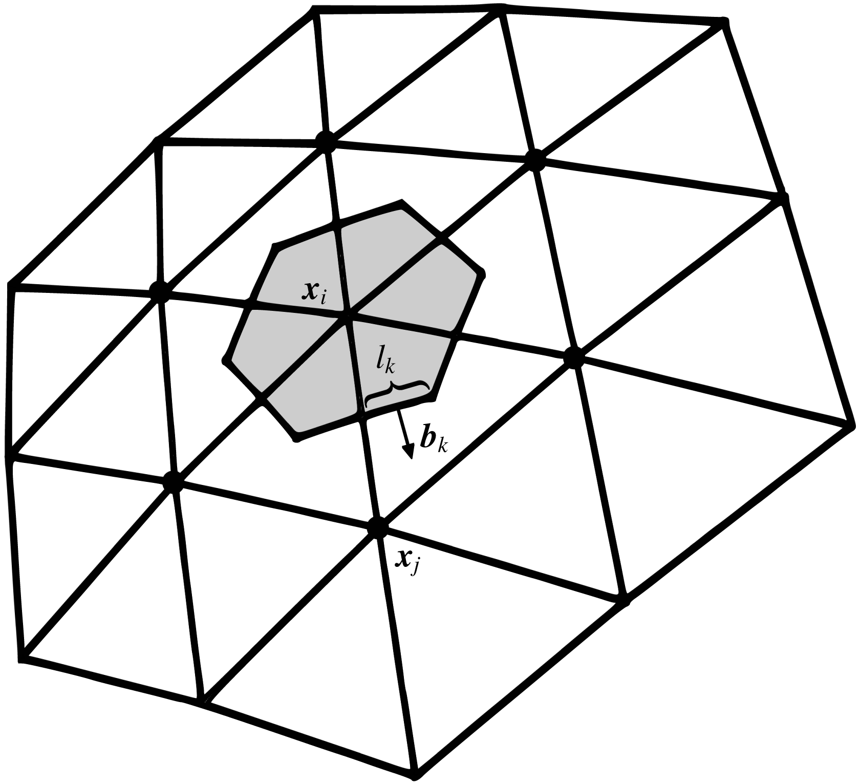
The integral form of (4.1) results in a finite-volume formulation of surfactant transport. In this formulation, the surfactant concentration at each node is updated using the sum of concentration fluxes through the faces of the dual mesh. A typical dual cell is illustrated in figure 2. The contour
 $C_{i}$
of the dual-mesh cell
 $S_{i}$
around node
 $\boldsymbol{x}_{i}$
of the triangle mesh is formed by the edge midpoints of triangles sharing node
 $\boldsymbol{x}_{i}$
and triangle centroids, as shown in figure 2. As introduced by Yon & Pozrikidis (Reference Yon and Pozrikidis1998), after neglecting diffusion, this refactoring results in the balance
 $$\begin{eqnarray}\int _{S_{i}}\frac{\text{d}\unicode[STIX]{x1D6E4}}{\text{d}t}\,\text{d}S=\int _{S_{i}}(\boldsymbol{w}+\boldsymbol{u})\boldsymbol{\cdot }\unicode[STIX]{x1D735}_{s}\unicode[STIX]{x1D6E4}\,\text{d}S-\int _{S_{i}}\unicode[STIX]{x1D735}_{s}\boldsymbol{\cdot }(\unicode[STIX]{x1D6E4}\boldsymbol{u})\,\text{d}S-2\int _{S_{i}}\unicode[STIX]{x1D6E4}k\boldsymbol{u}\boldsymbol{\cdot }\boldsymbol{n}\,\text{d}S.\end{eqnarray}$$
A typical dual-mesh cell
 $S_{i}$
(shaded grey) used for finite-volume formulations of surfactant transport. Surfactant flux through cell edges determines the change in concentration at a node
 $\boldsymbol{x}_{i}$
, influenced by neighbouring nodes
 $\boldsymbol{x}_{j}$
. The dual-cell contour is defined by edge midpoints and triangle centroids. A contour segment has length
 $l_{k}$
, and its unit normal
 $\boldsymbol{b}_{k}$
is in the plane of its containing triangle.

Converting (4.4) into numerical form, as provided by Bazhlekov et al. (Reference Bazhlekov, Anderson and Meijer2003), results in the following discrete terms:
 $$\begin{eqnarray}\int _{S_{i}}(\boldsymbol{w}+\boldsymbol{u})\boldsymbol{\cdot }\unicode[STIX]{x1D735}_{s}\unicode[STIX]{x1D6E4}\,\text{d}S\approx \frac{1}{3}(\boldsymbol{w}+\boldsymbol{u})_{i}\boldsymbol{\cdot }\mathop{\sum }_{j\in N_{i}^{T}}(\unicode[STIX]{x1D735}_{s}\unicode[STIX]{x1D6E4})_{j}{\mathcal{A}}_{j},\end{eqnarray}$$
where the subscript
 $i$
denotes values at node
 $i$
,
 $N_{i}^{T}$
is the set of triangles containing node
 $i$
,
 ${\mathcal{A}}_{j}$
is the area of the
 $j$
th triangle and
 $\unicode[STIX]{x1D6E4}$
in each triangle is a linear interpolation of the nodal values,
 $$\begin{eqnarray}\int _{S_{i}}\unicode[STIX]{x1D735}_{s}\boldsymbol{\cdot }(\unicode[STIX]{x1D6E4}\boldsymbol{u})\,\text{d}S=\int _{C_{i}}\unicode[STIX]{x1D6E4}\boldsymbol{u}\boldsymbol{\cdot }\boldsymbol{b}\,\text{d}C\approx \mathop{\sum }_{k}\left(\boldsymbol{b}_{k}\boldsymbol{\cdot }\int _{{\mathcal{L}}_{k}}\unicode[STIX]{x1D6E4}\boldsymbol{u}\,\text{d}l\right),\end{eqnarray}$$
where the summation is over all straight contour segments
 ${\mathcal{L}}_{k}$
in
 $C_{i}$
(two per mesh triangle),
 $\boldsymbol{b}_{k}$
is the outward unit normal to segment
 ${\mathcal{L}}_{k}$
of length
 $l_{k}$
(see figure 2), values at contour segment endpoints are determined from a linear interpolation within their containing mesh triangle, the integral on the right-hand side of (4.6) is calculated using the trapezoid rule, and
 $$\begin{eqnarray}\int _{S_{i}}\unicode[STIX]{x1D6E4}k\boldsymbol{u}\boldsymbol{\cdot }\boldsymbol{n}\,\text{d}S\approx \unicode[STIX]{x1D6E4}_{i}k_{i}(\boldsymbol{u}_{i}\boldsymbol{\cdot }\boldsymbol{n}_{i})S_{i},\end{eqnarray}$$
with the dual-cell area
 $$\begin{eqnarray}S_{i}=\frac{1}{3}\mathop{\sum }_{j\in N_{i}^{T}}{\mathcal{A}}_{j}.\end{eqnarray}$$
The numerical form of the convection equation can be written as a system of equations
 $$\begin{eqnarray}\frac{\text{d}\unicode[STIX]{x1D6E4}_{i}}{\text{d}t}=\mathop{\sum }_{j\in (N_{i}\cup i)}A_{ij}\unicode[STIX]{x1D6E4}_{j},\quad i=1,2,\ldots ,N,\end{eqnarray}$$
where
 $A_{ij}$
coefficients are a function of given node positions and velocities,
 $N_{i}$
is the set of neighbouring mesh nodes (see figure 2) and
 $N$
is the total number of drop mesh nodes. It is straightforward to study various time integration methods for (4.9) via the theta method,
 $$\begin{eqnarray}\unicode[STIX]{x1D6E4}_{i}(t+\unicode[STIX]{x0394}t)=\unicode[STIX]{x1D6E4}_{i}(t)+\unicode[STIX]{x0394}t\mathop{\sum }_{j\in (N_{i}\cup i)}A_{ij}\boldsymbol{\cdot }[\unicode[STIX]{x1D703}\unicode[STIX]{x1D6E4}_{j}(t+\unicode[STIX]{x0394}t)+(1-\unicode[STIX]{x1D703})\unicode[STIX]{x1D6E4}_{j}(t)],\end{eqnarray}$$
where
 $\unicode[STIX]{x1D703}=0$
corresponds to Euler explicit time integration,
 $\unicode[STIX]{x1D703}=0.5$
to Crank–Nicholson, and
 $\unicode[STIX]{x1D703}=1$
to fully implicit. The Gauss–Seidel iteration was used to solve the system of equations when necessary.
The FV implementation tested here differs from that of Bazhlekov et al. (Reference Bazhlekov, Anderson and Meijer2003) in the calculation of mean curvature and surface normals. Rather than via contour integration, curvature and normal vectors are obtained by best paraboloid fitting (Zinchenko, Rother & Davis Reference Zinchenko, Rother and Davis1997). This method exploits the observation that a smooth interface may be locally approximated by quadratic surface. This distinction in methodology is important due to the large deformations experienced by a drop during tight squeezing, which result in significant deviation from its initial sphericity, including transient nearly flat areas. As noted by Zinchenko et al. (Reference Zinchenko, Rother and Davis1997), mean curvature calculation via paraboloid fitting eliminates difficulties inherent in the contour integration method and demonstrates superior convergence in the nearly flat and near-contact dimple regions that play a critical role in lubrication.
The primary objective of exploring alternative transport schemes is to stably treat low drop-to-medium viscosity ratios while sharply resolving regions of high gradient. Therefore, no attempt was made in the present work to incorporate artificial diffusion into the FV scheme. Instead, several types of time integration were investigated using high mesh resolutions (
 $\widetilde{N}_{\triangle }=20~\text{K}$
). Overall, this non-diffusive FV scheme was found to notably improve numerical stability near critical conditions. For example, simulations failed after a short time at
 $Ca=0.9$
,
 $\unicode[STIX]{x1D706}=0.25$
and
 $\unicode[STIX]{x1D6FD}=0.05$
when using the LS scheme (even with implicit time integration), but the FV version proceeded past the global minimum drop velocity before suffering from similar instabilities and mesh degradation near sharp concentration gradients. However, spurious oscillations in the surfactant concentration occasionally appeared during the onset of squeezing, usually immediately upwind from developing sharp gradients. These unphysical numerical artifacts were not eliminated by semi-implicit (Crank–Nicholson) or fully implicit time integration. Away from critical parameters, erroneous oscillations are minimal and the FV scheme proves to be a reliably stable method for purely non-diffusive surfactant transport.
4.3 Upwind FV scheme
Convection-dominated transport of compressible media can be modelled by a formulation biased toward the upwind contribution of the velocity field. Upwind schemes generally increase the stability of convected scalar fields that may contain sharp gradients, at the cost of introducing numerical diffusion that is dependent on mesh resolution. For an upwind version of the FV surfactant transport algorithm, we follow the ideas of first-order schemes from inviscid fluid modelling (Smolarkiewicz & Szmelter Reference Smolarkiewicz and Szmelter2005). In the present context, it is advantageous first to reformulate the non-diffusive form of the transport equation (4.1) for node
 $i$
using the reference frame translating with the nodal velocity
 $\boldsymbol{V}_{i}$
, and the corresponding relative fluid velocity
 $\boldsymbol{u}-\boldsymbol{V}_{i}$
near node
 $i$
. From the relation
 $\unicode[STIX]{x1D735}_{s}\boldsymbol{\cdot }\boldsymbol{C}=-2k\boldsymbol{C}\boldsymbol{\cdot }\boldsymbol{n}$
valid for any constant vector
 $\boldsymbol{C}$
on a surface, equation (4.1) can be formally rewritten as
 $$\begin{eqnarray}\frac{\text{d}\unicode[STIX]{x1D6E4}}{\text{d}t}=\boldsymbol{w}\boldsymbol{\cdot }\unicode[STIX]{x1D735}_{s}\unicode[STIX]{x1D6E4}-\unicode[STIX]{x1D735}_{s}\boldsymbol{\cdot }[\unicode[STIX]{x1D6E4}(\boldsymbol{u}-\boldsymbol{V}_{i})]+(\boldsymbol{u}-\boldsymbol{V}_{i})\boldsymbol{\cdot }\unicode[STIX]{x1D735}_{s}\unicode[STIX]{x1D6E4}+2k\unicode[STIX]{x1D6E4}(\boldsymbol{V}_{i}-\boldsymbol{u})\boldsymbol{\cdot }\boldsymbol{n}\end{eqnarray}$$
at node
 $i$
(on the understanding that
 $\boldsymbol{V}_{i}$
is treated as constant in the differential operation of (4.11)). The last term in (4.11) vanishes, since the nodal velocity
 $\boldsymbol{V}_{i}=\text{d}\boldsymbol{x}_{i}/\text{d}t$
is constructed to always have the same normal component as the fluid velocity
 $\boldsymbol{u}$
for correct drop shape evolution. Recollecting the definition
 $\boldsymbol{V}=\boldsymbol{u}+\boldsymbol{w}$
brings (4.11) to the simple form
 $$\begin{eqnarray}\frac{\text{d}\unicode[STIX]{x1D6E4}}{\text{d}t}=-\unicode[STIX]{x1D735}_{s}\boldsymbol{\cdot }(\unicode[STIX]{x1D6E4}(\boldsymbol{u}-\boldsymbol{V}_{\boldsymbol{i}}))\end{eqnarray}$$
at node
 $i$
. Using (4.12) not only eliminates the need for curvature calculation (which could be unsatisfactory with some methods), but was also found in the present work to improve stability of the surfactant transport scheme.
Based on the integral form of (4.12), the surfactant concentration at node
 $i$
is updated as
 $$\begin{eqnarray}\unicode[STIX]{x1D6E4}_{i}^{n+1}=\unicode[STIX]{x1D6E4}_{i}^{n}-\frac{\unicode[STIX]{x0394}t}{S_{i}}\mathop{\sum }_{k}F_{k}^{\bot }l_{k},\end{eqnarray}$$
where the summation is, again, over all straight contour segments
 ${\mathcal{L}}_{k}$
with length
 $l_{k}$
and
 $F_{k}^{\bot }$
is the normal flux of
 $\unicode[STIX]{x1D6E4}$
through
 ${\mathcal{L}}_{k}$
per unit length. Let
 $(\boldsymbol{x}_{i}+\boldsymbol{x}_{j})/2$
be the mesh edge midpoint associated with
 ${\mathcal{L}}_{k}$
(figure 2) and
 $$\begin{eqnarray}v^{\bot }=[{\textstyle \frac{1}{2}}(\boldsymbol{u}_{i}+\boldsymbol{u}_{j})-\boldsymbol{V}_{i}]\boldsymbol{\cdot }\boldsymbol{b}_{k}\end{eqnarray}$$
be the approximation for the relative velocity component
 $(\boldsymbol{u}-\boldsymbol{V}_{i})\boldsymbol{\cdot }\boldsymbol{b}_{k}$
on
 ${\mathcal{L}}_{k}$
. Following the pattern of upwind schemes, the flux calculation depends on the sign of
 $v^{\bot }$
:
 $$\begin{eqnarray}F_{k}^{\bot }=[v^{\bot }]^{+}\unicode[STIX]{x1D6E4}_{i}^{n}+[v^{\bot }]^{-}\unicode[STIX]{x1D6E4}_{j}^{n},\end{eqnarray}$$
where, in general,
 $$\begin{eqnarray}[v]^{+}\equiv 0.5(v+|v|),\quad [v]^{-}\equiv 0.5(v-|v|).\end{eqnarray}$$
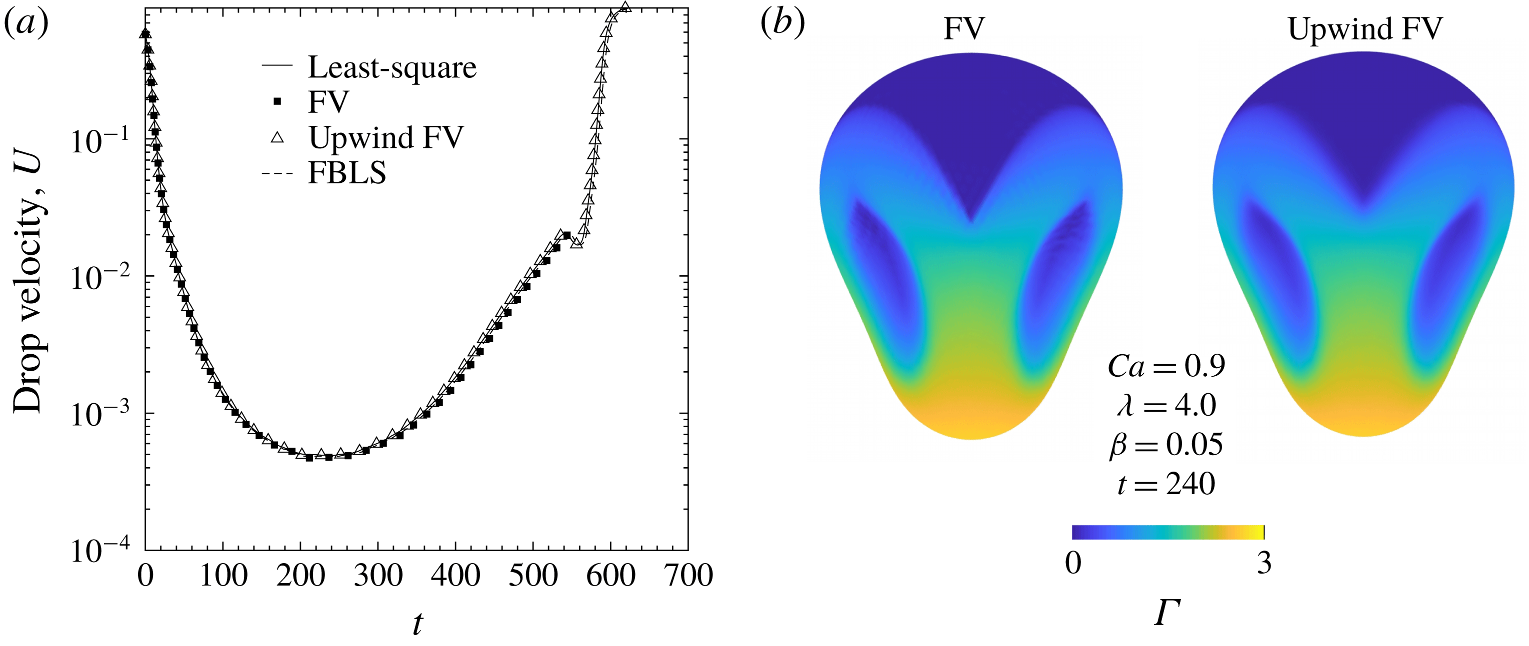
Many advanced upwind schemes have been developed for inviscid fluid modelling in order to treat high-Reynolds-number compressible flows, which may contain large density gradients or time-dependent shock waves. In the present quasi-steady-state regime, it is unlikely that higher-order schemes will significantly increase the accuracy with respect to drop squeezing dynamics. The above first-order upwind FV scheme for unstructured meshes was found to be in close agreement with both LS and strictly conservative FV formulations at moderately high viscosity ratios, even near critical squeezing conditions (see figure 3 and § 5). It is therefore used to predict the squeezing behaviour at more extreme viscosity ratios that previous implementations have been unable to model. Euler explicit time integration was used for all upwind FV simulations.
Convergence of drop velocity for different surfactant transport schemes, with
 $Ca=0.9$
,
 $\unicode[STIX]{x1D706}=4.0$
,
 $\unicode[STIX]{x1D6FD}=0.05$
,
 $\widetilde{N}_{\triangle }=20~\text{K}$
,
 $\widehat{N}_{\triangle }=8.6~\text{K}$
. (a) All schemes converge with respect to drop velocity versus time, near the critical capillary number. (b) Surfactant concentration distributions at the global velocity minimum; the upwind finite-volume method stably captures surfactant behaviour.

4.4 Flow-biased least-squares (FBLS) scheme
We have found most recently that the stability of the simple least-squares method of Zinchenko & Davis (Reference Zinchenko and Davis2017a
) for the transport equation (4.1) can also be greatly increased by reducing the order of approximation for
 $\boldsymbol{w}\boldsymbol{\cdot }\unicode[STIX]{x1D735}_{s}\unicode[STIX]{x1D6E4}$
(the convective term primarily responsible for stability), instead of introducing artificial diffusion
 $D_{s}$
. In the intrinsic coordinate system
 $(x_{1}^{\prime },x_{2}^{\prime },x_{3}^{\prime })$
centred at node
 $\boldsymbol{O}$
, with the
 $x_{3}^{\prime }$
-axis along the normal vector
 $\boldsymbol{n}_{\boldsymbol{O}}$
(here and below, subscript
 $\boldsymbol{O}$
relates to quantities at node
 $\boldsymbol{O}$
), the surface can be approximated as a paraboloid
 $x_{3}^{\prime }=C(x_{1}^{\prime })^{2}+Dx_{1}^{\prime }x_{2}^{\prime }+E(x_{2}^{\prime })^{2}$
near
 $\boldsymbol{O}$
, which gives local parameterization in terms of
 $x_{1}^{\prime }$
and
 $x_{2}^{\prime }$
. As in Zinchenko & Davis (Reference Zinchenko and Davis2017a
), quadratic polynomials are used to approximate the first two intrinsic fluid velocity components
 $u_{\unicode[STIX]{x1D6FC}}^{\prime }$
(
 $\unicode[STIX]{x1D6FC}=1,2$
) near
 $\boldsymbol{O}$
:
 $$\begin{eqnarray}u_{\unicode[STIX]{x1D6FC}}^{\prime }(x_{1}^{\prime },x_{2}^{\prime })=(u_{\unicode[STIX]{x1D6FC}}^{\prime })_{\boldsymbol{ O}}+a_{\unicode[STIX]{x1D6FC}}x_{1}^{\prime }+b_{\unicode[STIX]{x1D6FC}}x_{2}^{\prime }+c_{\unicode[STIX]{x1D6FC}}(x_{1}^{\prime })^{2}+d_{\unicode[STIX]{x1D6FC}}x_{1}^{\prime }x_{2}^{\prime }+e_{\unicode[STIX]{x1D6FC}}(x_{2}^{\prime })^{2}.\end{eqnarray}$$
The five coefficients
 $a_{\unicode[STIX]{x1D6FC}}\cdots e_{\unicode[STIX]{x1D6FC}}$
are found by least-squares fitting of (4.17) to the values of
 $u_{\unicode[STIX]{x1D6FC}}^{\prime }$
for the whole set
 ${\mathcal{A}}$
of mesh nodes
 $\boldsymbol{x}_{j}$
directly connected to
 $\boldsymbol{O}$
. This fitting is well-defined, since the coordination number of any node
 $\boldsymbol{O}$
for our meshes is at least five (typically six). The divergence and curvature terms in (4.1) combine to (Zinchenko & Davis Reference Zinchenko and Davis2017a
)
 $$\begin{eqnarray}-\unicode[STIX]{x1D6E4}_{\boldsymbol{O}}(\unicode[STIX]{x1D735}_{s}\boldsymbol{\cdot }\boldsymbol{u}+2k\boldsymbol{u}\boldsymbol{\cdot }\boldsymbol{n})_{\boldsymbol{O}}=-\unicode[STIX]{x1D6E4}_{\boldsymbol{O}}(a_{1}+b_{2}),\end{eqnarray}$$
so this method, again, does not require curvature calculation.
For surfactant concentration, in contrast, a local linear approximation is used,
 $$\begin{eqnarray}\unicode[STIX]{x1D6E4}(x_{1}^{\prime },x_{2}^{\prime })=\unicode[STIX]{x1D6E4}_{\boldsymbol{ O}}+Ax_{1}^{\prime }+Bx_{2}^{\prime },\end{eqnarray}$$
with coefficients
 $A$
and
 $B$
required to provide the least-squares fit of (4.19) to
 $\unicode[STIX]{x1D6E4}$
-values in the selected subset (see below)
 ${\mathcal{A}}_{sel}\subset {\mathcal{A}}$
of mesh nodes around
 $\boldsymbol{O}$
:
 $$\begin{eqnarray}\mathop{\sum }_{j\in {\mathcal{A}}_{sel}}[A(x_{j}^{\prime })_{1}+B(x_{j}^{\prime })_{2}-\unicode[STIX]{x0394}\unicode[STIX]{x1D6E4}_{j}]^{2}\rightarrow \min ,\quad \unicode[STIX]{x0394}\unicode[STIX]{x1D6E4}_{j}=\unicode[STIX]{x1D6E4}(\boldsymbol{x}_{j})-\unicode[STIX]{x1D6E4}_{\boldsymbol{O}}.\end{eqnarray}$$
The fitting operation (4.19)–(4.20) requires
 ${\mathcal{A}}_{sel}$
to include at least two neighbours. Let the excess velocity
 $\boldsymbol{w}_{\boldsymbol{O}}$
be
 $(w_{1}^{\prime },w_{2}^{\prime },0)$
in the intrinsic basis. Solving (4.20) for
 $A$
and
 $B$
, the convection term can be written as
 $$\begin{eqnarray}(\boldsymbol{w}\boldsymbol{\cdot }\unicode[STIX]{x1D735}_{s}\unicode[STIX]{x1D6E4})_{\boldsymbol{O}}=\mathop{\sum }_{j\in {\mathcal{A}}_{sel}}\unicode[STIX]{x1D707}_{j}\unicode[STIX]{x0394}\unicode[STIX]{x1D6E4}_{j},\end{eqnarray}$$
with the coefficients
 $$\begin{eqnarray}\unicode[STIX]{x1D707}_{j}=\frac{w_{1}^{\prime }[(x_{j}^{\prime })_{1}T_{22}-(x_{j}^{\prime })_{2}T_{12}]+w_{2}^{\prime }[T_{11}(x_{j}^{\prime })_{2}-T_{12}(x_{j}^{\prime })_{1}]}{T_{11}T_{22}-T_{12}^{2}}\end{eqnarray}$$
and
 $$\begin{eqnarray}T_{\unicode[STIX]{x1D6FC}\unicode[STIX]{x1D6FD}}=\mathop{\sum }_{j\in {\mathcal{A}}_{sel}}(x_{j}^{\prime })_{\unicode[STIX]{x1D6FC}}(x_{j}^{\prime })_{\unicode[STIX]{x1D6FD}}.\end{eqnarray}$$
A standard, rigorously derived stability requirement for surfactant update
 $$\begin{eqnarray}\unicode[STIX]{x1D6E4}_{\boldsymbol{O}}^{n+1}=\unicode[STIX]{x1D6E4}_{\boldsymbol{ O}}^{n}+\unicode[STIX]{x0394}t\mathop{\sum }_{j\in {\mathcal{A}}_{sel}}\unicode[STIX]{x1D707}_{j}(\unicode[STIX]{x1D6E4}_{j}^{n}-\unicode[STIX]{x1D6E4}_{\boldsymbol{ O}}^{n})+\cdots\end{eqnarray}$$
is
 $\unicode[STIX]{x1D707}_{j}>0$
for all
 $j\in {\mathcal{A}}_{sel}$
(at sufficiently small
 $\unicode[STIX]{x0394}t$
). Accordingly, to construct
 ${\mathcal{A}}_{sel}$
, we start from all neighbours (
 ${\mathcal{A}}_{sel}={\mathcal{A}}$
), calculate
 $\unicode[STIX]{x1D707}_{j}$
from (4.22)–(4.23) and exclude the neighbour
 $j$
with the most negative
 $\unicode[STIX]{x1D707}_{j}$
. The calculations (4.22)–(4.23) are then repeated, if necessary, for the reduced set
 ${\mathcal{A}}_{sel}$
to find and exclude another neighbour
 $j$
with the most negative
 $\unicode[STIX]{x1D707}_{j}$
, etc., until the set
 ${\mathcal{A}}_{sel}$
is achieved with all positive
 $\unicode[STIX]{x1D707}_{j}$
. This logic can sometimes reduce
 ${\mathcal{A}}_{sel}$
to two neighbours, with one
 $\unicode[STIX]{x1D707}_{j}$
still negative; in this case, node selection is forcefully terminated at two neighbours left to calculate the convective term, notwithstanding
 $\unicode[STIX]{x1D707}_{j}<0$
. Such events were extremely rare in our simulations and did not jeopardize stability. On average, the set
 ${\mathcal{A}}_{sel}$
is observed to contain three neighbours. Also note that
 $\unicode[STIX]{x1D707}_{j}>0$
is not the same as the intuitive upwind condition
 $w_{1}^{\prime }(x_{j}^{\prime })_{1}+w_{2}^{\prime }(x_{j}^{\prime })_{2}>0$
. The FBLS method is quite simple in terms of programming and agrees well with all tested convection schemes at high viscosity ratio near critical conditions (figure 3). Moreover, this scheme is stable at all parameter sets of interest and was used to complement, and as an additional validation of, the upwind FV method; at low viscosity ratios (
 $Ca=1.1,\unicode[STIX]{x1D706}=0.1,\unicode[STIX]{x1D6FD}=0.05$
), squeezing times agree to within
 ${\sim}2\,\%$
at resolutions of
 $\widetilde{N}_{\triangle }=15.4~\text{K}$
and
 $\widehat{N}_{\triangle }=11.5~\text{K}$
(see § 5.3 for more comparisons).
5 Numerical results
All values from the numerical simulations of contaminated-drop tight squeezing are reported in non-dimensional form. The characteristic length scale
 $L$
is taken as the solid-particle radius
 $\widehat{a}$
. The velocity and times scales are
 $|\boldsymbol{u}_{\infty }|$
and
 $L/|\boldsymbol{u}_{\infty }|$
, respectively. Surface tension and surfactant concentration at the drop surface are scaled with their equilibrium values, where equilibrium (
 $eq$
) is defined as the case of uniform surfactant concentration on a spherical drop:
 $$\begin{eqnarray}\unicode[STIX]{x1D6E4}^{\ast }=\unicode[STIX]{x1D6E4}/\unicode[STIX]{x1D6E4}_{eq},\quad \unicode[STIX]{x1D70E}^{\ast }=\unicode[STIX]{x1D70E}/\unicode[STIX]{x1D70E}_{eq}.\end{eqnarray}$$
For the entirety of this section, the superscript
 $^{\ast }$
will be dropped for conciseness. The Hebeker parameter
 $\unicode[STIX]{x1D702}$
in the boundary-integral formulation (3.1)–(3.2) is set to unity. The initial drop shape is spherical, far upstream from the constriction and covered in uniformly distributed surfactant. Definitions of
 $Ca$
,
 $\unicode[STIX]{x1D706}$
and
 $\unicode[STIX]{x1D6FD}$
are provided in § 2.
5.1 Numerical convergence tests
Most simulations were completed with high mesh resolutions (
 $\widetilde{N}_{\triangle }:~15.4~\text{K}-20~\text{K}$
,
 $\widehat{N}_{\triangle }:~11.5~\text{K}-20~\text{K}$
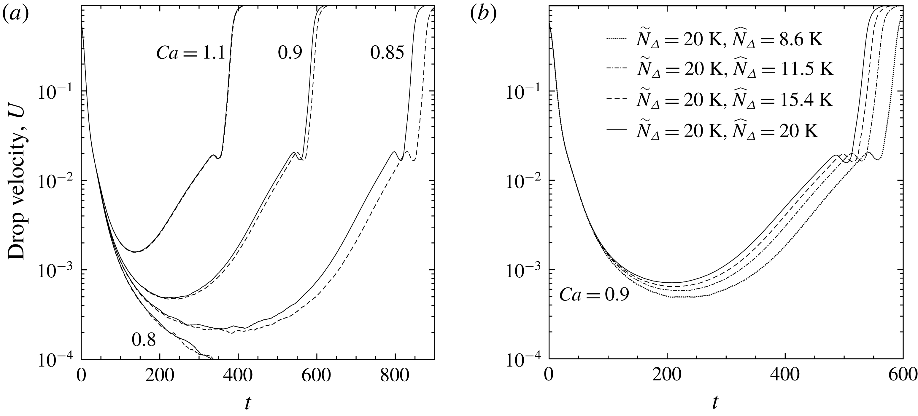
) for accurate drop-squeezing simulations. The effect of drop triangulation with the LS method for surfactant transport is shown in figure 4. Away from critical conditions there is a negligible dependence of squeezing dynamics on drop mesh resolution for
 $\widetilde{N}_{\triangle }\geqslant 11.5~\text{K}$
. Closer to critical
 $Ca$
(
 $Ca_{crit}$
, discussed below), the effect of drop triangulation becomes more significant but remains acceptable (see figure 4
a,
 $Ca=0.9,0.85$
). Near critical conditions, squeezing times are more sensitive to particle mesh resolution, as shown for
 $Ca=0.9$
in figure 4(b). While we often made use of higher resolutions in the following results, generally
 $\widehat{N}_{\triangle }\geqslant 11.5~\text{K}$
is deemed acceptable. Excellent agreement between all tested convection schemes is observed at moderate-to-high viscosity ratios, for which all tested methods are stable (figure 3
a). To confirm convergence at low viscosity ratio, where not all convection schemes can be tested, a high-resolution (
 $\widetilde{N}_{\triangle }=20~\text{K}$
,
 $\widehat{N}_{\triangle }=20~\text{K}$
) run was completed using the upwind FV scheme at near-critical conditions (
 $Ca=0.9,\unicode[STIX]{x1D706}=0.1,\unicode[STIX]{x1D6FD}=0.05$
). The drop squeezing time agrees to within
 ${<}1.0\,\%$
with the ‘standard’ resolution (
 $\widetilde{N}_{\triangle }=15.4~\text{K}$
,
 $\widehat{N}_{\triangle }=11.5~\text{K}$
) result. In addition, close agreement is found between the results by upwind FV and FBLS schemes (see § 5.3); these are the only two stable schemes for squeezing simulations at small
 $\unicode[STIX]{x1D706}$
.
Convergence of results with respect to mesh resolution (
 $\unicode[STIX]{x1D706}=4.0,\unicode[STIX]{x1D6FD}=0.05$
). (a) Solid lines (
 $\widetilde{N}_{\triangle }=20~\text{K},\widehat{N}_{\triangle }=8.6~\text{K}$
), and dashed lines (
 $\widetilde{N}_{\triangle }=11.5~\text{K},\widehat{N}_{\triangle }=8.6~\text{K}$
) show that the effect of droplet mesh resolution with the least-squares scheme is negligible except at near-critical conditions. (b) Convergence of drop velocity with respect to solid-particle triangulation at slightly supercritical
 $Ca$
.

The effect of initial droplet position, including vertical distance and horizontal offset from the constriction centre, on squeezing behaviour was quantified. Doubling the initial vertical offset (from the default 6) to 12 had no measurable effect on squeezing times for the range of
 $\unicode[STIX]{x1D6FD}$
used in this study, even at near-critical conditions (
 $Ca=0.9$
,
 $\unicode[STIX]{x1D706}=4.0$
). This result is consistent with the fact that the maximum local change in surface tension is small (
 ${\approx}0.1\,\%$
) in the first time step, for the default initial position. When the drop is initially placed with a horizontal offset from the constriction centre, there is a strong inclination for it to bypass the solid particles altogether. For example, using the default initial separation but shifting the drop halfway (or even quarterway) from directly above the constriction to directly above a spherical particle, results in the drop flowing around the three spheres. When offsetting the drop one eighth of this distance, the drop collides with the particle before moving into the constriction and quickly relaxing into its familiar shape. Due to this relatively fast drop relaxation, the minimum drop velocity and surfactant distribution at this point are negligibly affected, but squeezing times are increased due to slower droplet approach.
5.2 Capillary number
The evolution of surfactant on the surface of a tight-squeezing drop is shown in figure 5. The system represents behaviour at low drop contamination
 $\unicode[STIX]{x1D6FD}=0.05$
, moderately high viscosity ratio
 $\unicode[STIX]{x1D706}=4.0$
and slightly supercritical capillary number
 $Ca=0.9$
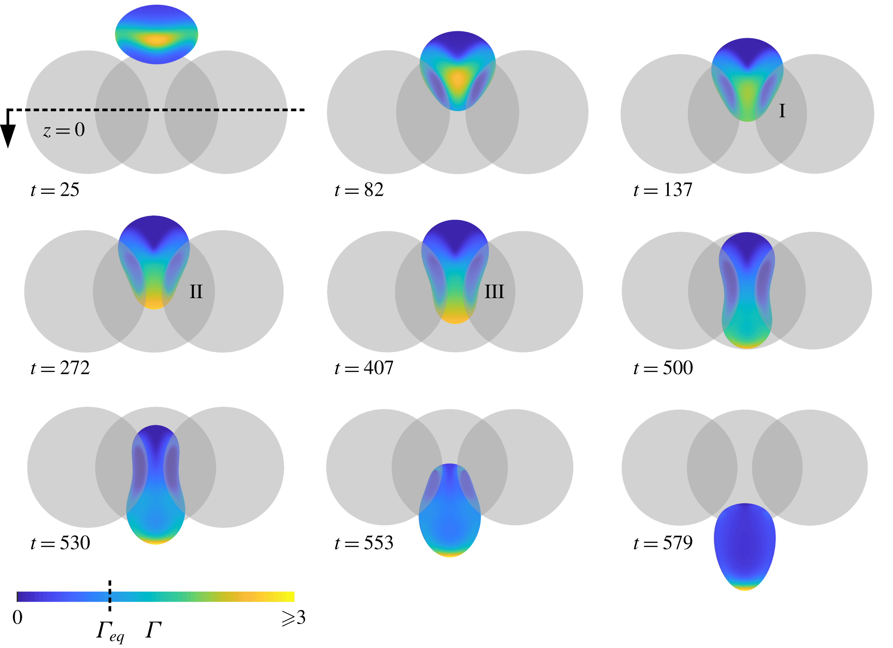
. The drop is subject to compressional flow as it approaches the constriction, and the initially uniformly distributed surfactant is advected toward the drop’s equator. Surfactant predominately concentrates above the interstices of the solid particles, where densities reach approximately three times the equilibrium value. Marangoni stresses resist further accumulation in these regions and, at this moderate-to-high viscosity ratio, prevent the formation of steep concentration gradients until the drop has begun to enter the constriction. By
 $t=82$
, the drop has nearly coated the solid obstacles. Due to the drop being driven by a uniform far-field flow, rather than settling under gravity, internal circulation develops that allows for diverging surface flow. Near-zero surfactant concentrations develop quickly on both the upstream-facing (top) surface and in the dimple regions of the drop, falling below
 $\unicode[STIX]{x1D6E4}\sim 10^{-3}$
by
 $t\sim 95$
and decreasing to
 $\unicode[STIX]{x1D6E4}<10^{-5}$
by
 $t=272$
. While Marangoni stresses tend to make the transition between depleted and concentrated regions more diffuse, they are unable to refill depleted areas until long after the drop has exited the constriction. A clean drop (
 $\unicode[STIX]{x1D6FD}=0$
) with otherwise equivalent parameters would be subcritical at
 $Ca=0.9$
, resulting in a trapped state. The mechanism by which the critical capillary number is decreased by drop contamination is summarized by snapshots I, II and III in figure 5. At
 $t=137$
, the drop reaches a position and shape similar to that of a trapped clean drop. The surfactant that has collected above interparticle interstices is gradually swept downwind by the inner-constriction flow field. Surfactant accumulates at the downwind pole, locally decreasing surface tension and enhancing deformation and elongation of the drop tip. Once the leading edge of the drop successfully passes through the constriction the remainder of the drop is able to follow. The drop exits the constriction with a highly non-uniform surface tension, with almost all surfactant located at the leading tip. While the trailing end is still near the constriction centre, such as at
 $t=553$
, the droplet develops into a shape similar to a pendant drop. During this stage, surfactant concentrations at the leading tip increase to eight times the original concentration, as seen in figure 6(d). Far downstream, the drop returns to spherical with uniform surfactant concentration.
Contaminated-drop squeezing through the three-sphere constriction (
 $Ca=0.9$
,
 $\unicode[STIX]{x1D706}=4.0$
,
 $\unicode[STIX]{x1D6FD}=0.05$
). The critical capillary number is decreased as compared to a clean drop. Near-critical contaminated-drop squeezing can be summarized by the stages
 $(\text{I})$
development of a typical trapped state,
 $(\text{II})$
surfactant accumulation at the downwind pole and
 $(\text{III})$
eventual elongation of the drop tip.

Effect of capillary number on contaminated-drop squeezing (
 $\unicode[STIX]{x1D706}=4.0$
,
 $\unicode[STIX]{x1D6FD}=0.05$
). Resolution for
 $Ca=1.5$
, 1.3 (
 $\widehat{N}_{\triangle }^{lo}$
):
 $\widetilde{N}_{\triangle }=20~\text{K}$
,
 $\widehat{N}_{\triangle }=8.6~\text{K}$
. Resolution for
 $Ca=1.1$
, 0.9 (
 $\widehat{N}_{\triangle }^{hi}$
):
 $\widetilde{N}_{\triangle }=20~\text{K}$
,
 $\widehat{N}_{\triangle }=20~\text{K}$
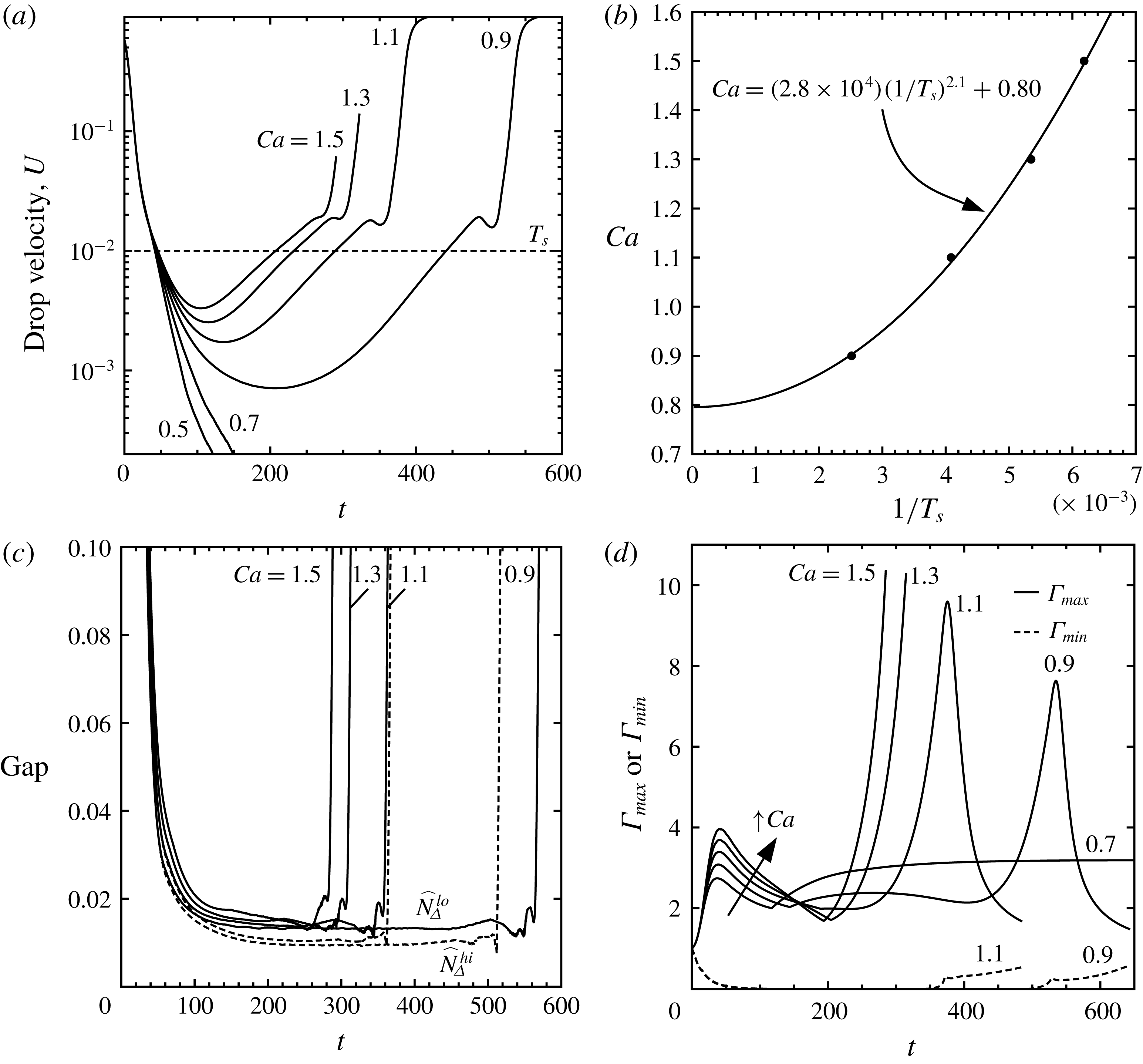
. (a) Drop dynamics under a range of sub-, super- and near-critical capillary numbers. Dashed tie line is used to define squeezing times. (b) Power-law fitting of supercritical squeezing times (●, numerical results) in order to extrapolate the critical value,
 $Ca=0.80$
. (c) Gap between drop and solid obstacles tends to decrease with capillary number. Dashed lines show effect of solid-particle resolution. (d) Evolution of surfactant concentrations for super- and subcritical
 $Ca$
. Cusps in global maximum surfactant concentration indicate when
 $\unicode[STIX]{x1D6E4}_{max}$
shifts to a different locale on the drop surface.

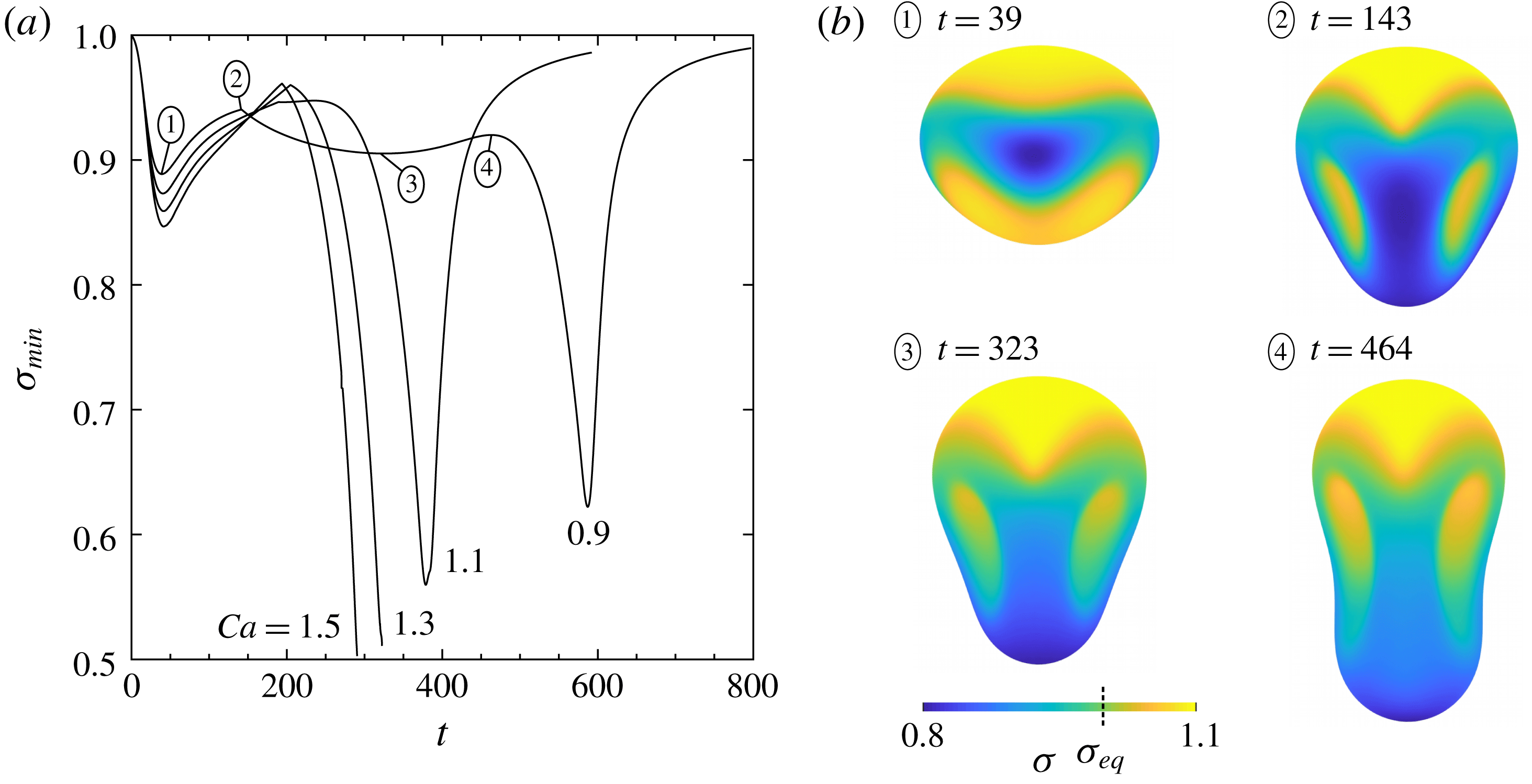
Evolution of surface tension during contaminated-drop squeezing through the three-sphere constriction (
 $\unicode[STIX]{x1D706}=4.0$
,
 $\unicode[STIX]{x1D6FD}=0.05$
,
 $\widetilde{N}_{\triangle }=15.4~\text{K}$
,
 $\widehat{N}_{\triangle }=11.5~\text{K}$
). (a) Global minimum value of surface tension. Labelled points on the
 $Ca=0.9$
curve are shown in (b). (b) Distribution of surface tension at various local extrema of
 $\unicode[STIX]{x1D70E}_{min}(t)$
at
 $Ca=0.9$
. Solid particles not shown.

As with clean drops, capillary number has a strong effect on contaminated-drop squeezing. The temporal dynamics in a wide range of capillary numbers are provided in figure 6, using high resolutions (
 $\widetilde{N}_{\triangle }=20~\text{K}$
,
 $\widehat{N}_{\triangle }=20~\text{K}$
) for the near-critical
 $Ca=0.9$
. As seen in figure 6(a), the critical capillary number (
 $Ca_{crit}$
), below which trapping occurs, is observed to lie between
 $Ca=0.7$
and
 $Ca=0.9$
. This value is consistent with a power-law regression of supercritical
 $Ca$
against squeezing time (
 $T_{s}$
) (a technique similar to that of Ratcliffe, Zinchenko & Davis (Reference Ratcliffe, Zinchenko and Davis2010) for gravity-induced squeezing), which predicts a
 $Ca_{crit}\approx 0.8$
(figure 6
b). In the present study, a squeezing drop is defined to have a velocity
 $U$
less than 1.0 % of the far-field velocity
 $|\boldsymbol{u}_{\infty }|$
. A similar analysis of previous work (Zinchenko & Davis Reference Zinchenko and Davis2006) indicates that
 $Ca_{crit}\approx 1.0$
for clean drops, corresponding to a
 ${\sim}20\,\%$
decrease in
 $Ca_{crit}$
at low degrees of contamination (
 $\unicode[STIX]{x1D6FD}=0.05$
) and moderately high viscosity ratios (
 $\unicode[STIX]{x1D706}=4.0$
). The minimum gap between drop and solid particles is a relatively weak function of capillary number and is similar to that for clean drops. Notably, for a contaminated drop, cusps in gap versus time are more pronounced at various stages of the squeezing process (cf. figure 6
c with figure 17 of Zinchenko & Davis (Reference Zinchenko and Davis2006)).
The global minimum value of surface tension (
 $\unicode[STIX]{x1D70E}_{min}$
) for a contaminated drop during the squeezing process is shown in figure 7(a). Discontinuities in the derivative of
 $\unicode[STIX]{x1D70E}_{min}(t)$
correspond to changes in the locale of maximum surfactant concentration, which occurs e.g. between
 $t=82$
and
 $t=272$
(figure 5). Decreasing capillary number tends to decrease the variation of
 $\unicode[STIX]{x1D70E}_{min}$
, which for
 $Ca=0.9$
remains between 5 % and 10 % less than
 $\unicode[STIX]{x1D70E}_{eq}$
for the majority of drop tight squeezing. The distribution of surface tension at local extrema of
 $\unicode[STIX]{x1D70E}_{min}(t)$
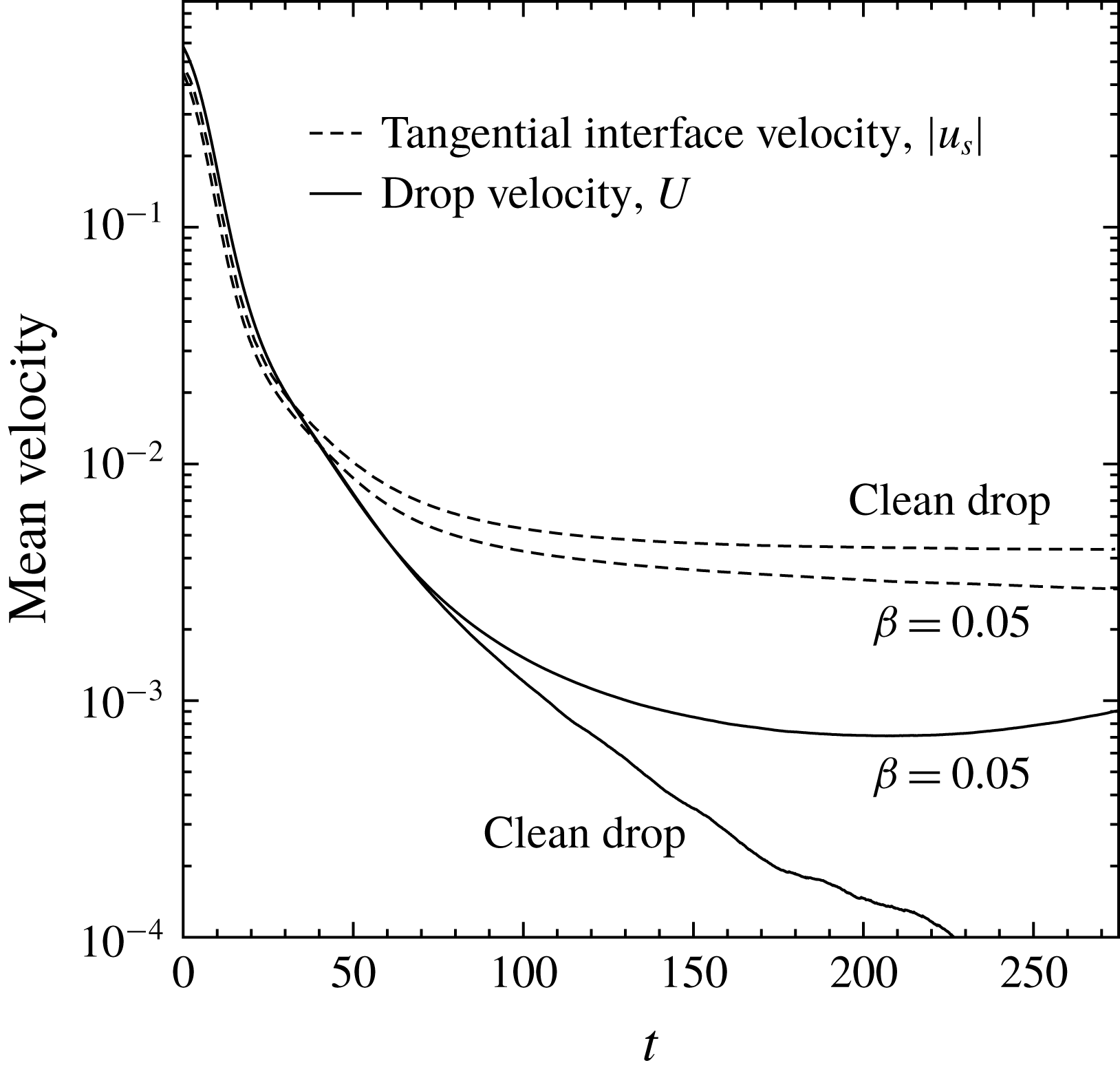
during the squeezing process is shown in figure 7(b). Notably, a linear equation of state appears sufficient to retain positive surface tension, despite the development of high surfactant concentrations. In conjunction with modifying local surface tension, the presence of surfactant is expected to affect surface mobility. A global metric for interface mobility can be defined as the surface average (
 $\overline{S}$
) of
 $|u_{s}|$
, where
 $u_{s}$
is the magnitude of the tangential fluid velocity
 $\boldsymbol{u}_{s}$
. As seen in figure 8, a trapped clean drop reaches a steady-state surface mobility (
 $|u_{s}|_{\overline{S}}$
) that is much higher than
 $U$
, due to internal circulation. Despite maintaining a higher
 $U$
during squeezing, a contaminated drop has lower surface mobility, as compared to a clean drop, due to Marangoni stresses resisting surface flow. However, the low degree of contamination (
 $\unicode[STIX]{x1D6FD}=0.05$
) is unable to completely immobilize the surface, driven by the far-field flow.
Effect of low surfactant contamination on drop interface mobility (
 $Ca=0.9$
,
 $\unicode[STIX]{x1D706}=4.0$
,
 $\widetilde{N}_{\triangle }=20~\text{K}$
,
 $\widehat{N}_{\triangle }=11.5~\text{K}$
), quantified as the surface average of
 $|u_{s}|$
, where
 $u_{s}$
is the magnitude of tangential velocity. The interface mobility of flow-driven tight-squeezing drops remains relatively high due to internal circulation. Surfactant decreases interface mobility due to the presence of resistive Marangoni stresses.

Effect of low surfactant contamination on the shape of steady-state trapped drops (
 $\unicode[STIX]{x1D706}=4.0$
,
 $\widetilde{N}_{\triangle }=20~\text{K}$
,
 $\widehat{N}_{\triangle }=11.5~\text{K}$
) at various capillary numbers. A moderately subcritical clean drop (
 $\unicode[STIX]{x1D6FD}=0.0,\unicode[STIX]{x1D6E4}_{eq}=0.0$
), for reference, is shaded to reveal 3D structure. A significantly lower
 $Ca$
is required for a similar contaminated-drop trapped shape. Dashed line indicates constriction centre. Drop is rotated to show dimpled face; solid particles not shown.

Several contaminated trapped states are compared to that of a moderately subcritical clean drop (
 $Ca=0.9$
) in figure 9 for
 $\unicode[STIX]{x1D706}=4.0$
. To obtain a similar trapped-drop shape at low surfactant loading,
 $Ca$
must be decreased to 0.7. A clean drop has
 $Ca_{crit}\approx 1.0$
, and the contaminated system has
 $Ca_{crit}\approx 0.8$
, so in both cases that characteristic shape is obtained when
 $Ca$
is
 ${\sim}0.1$
, less than
 $Ca_{crit}$
. For a near-critical contaminated drop such as for
 $Ca=0.8$
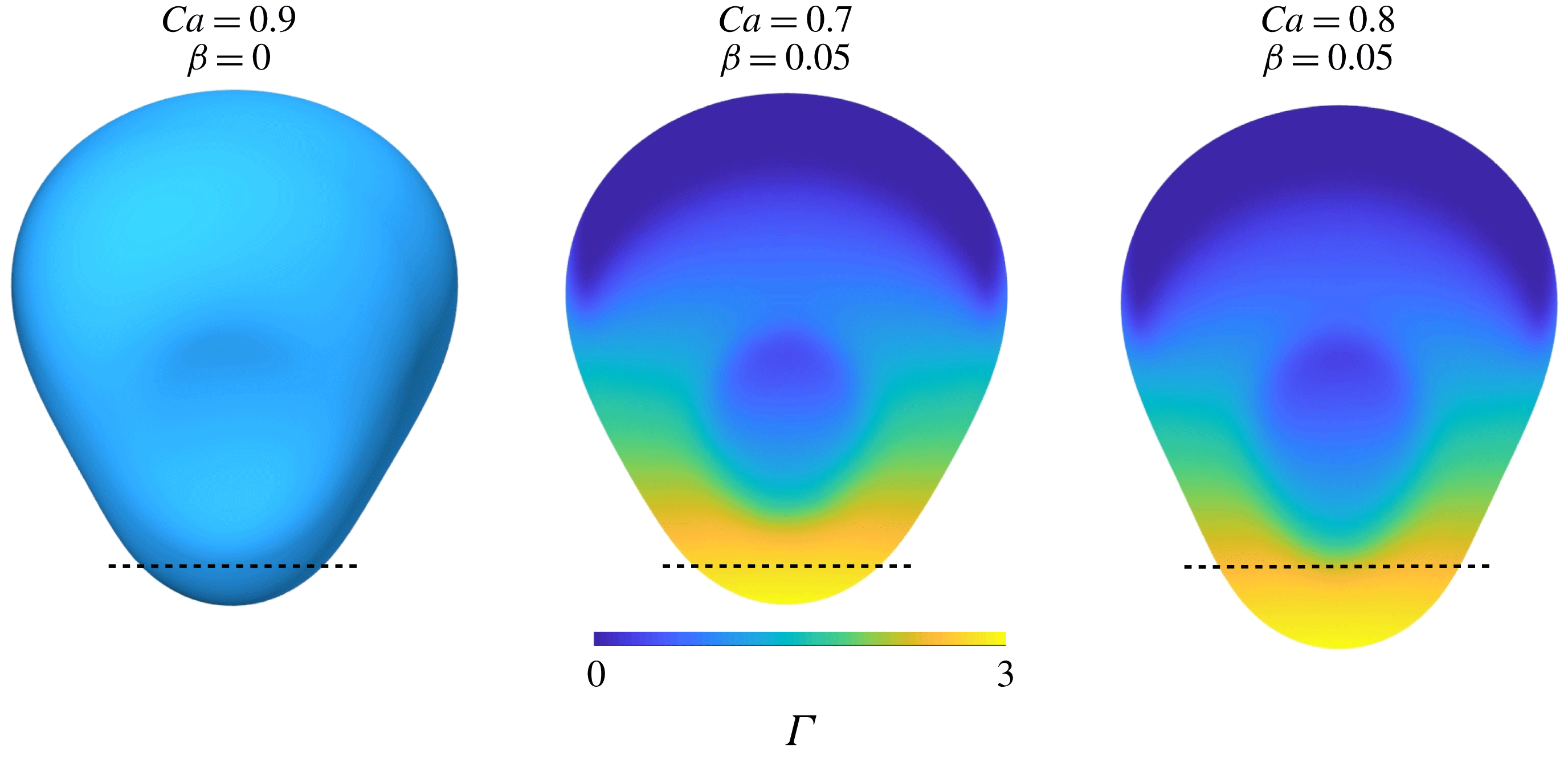
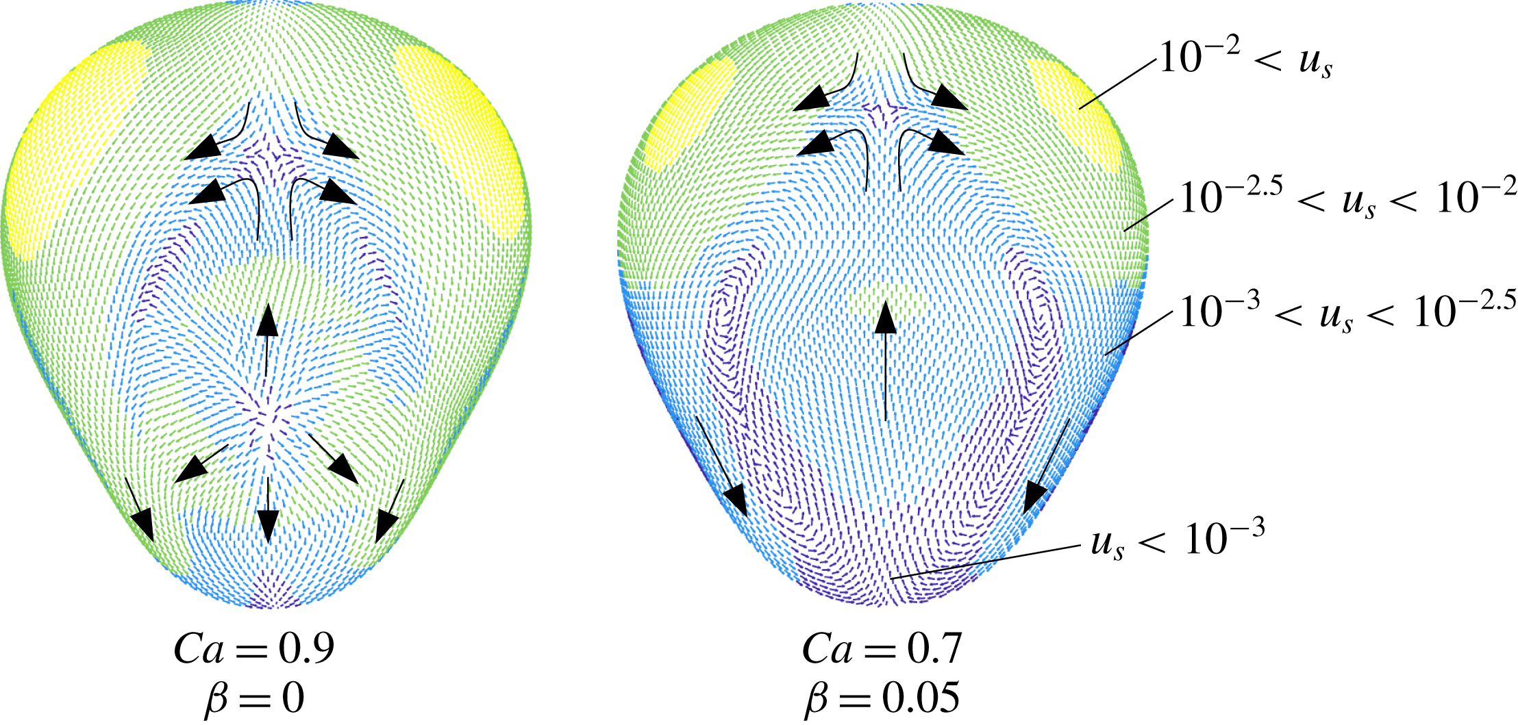
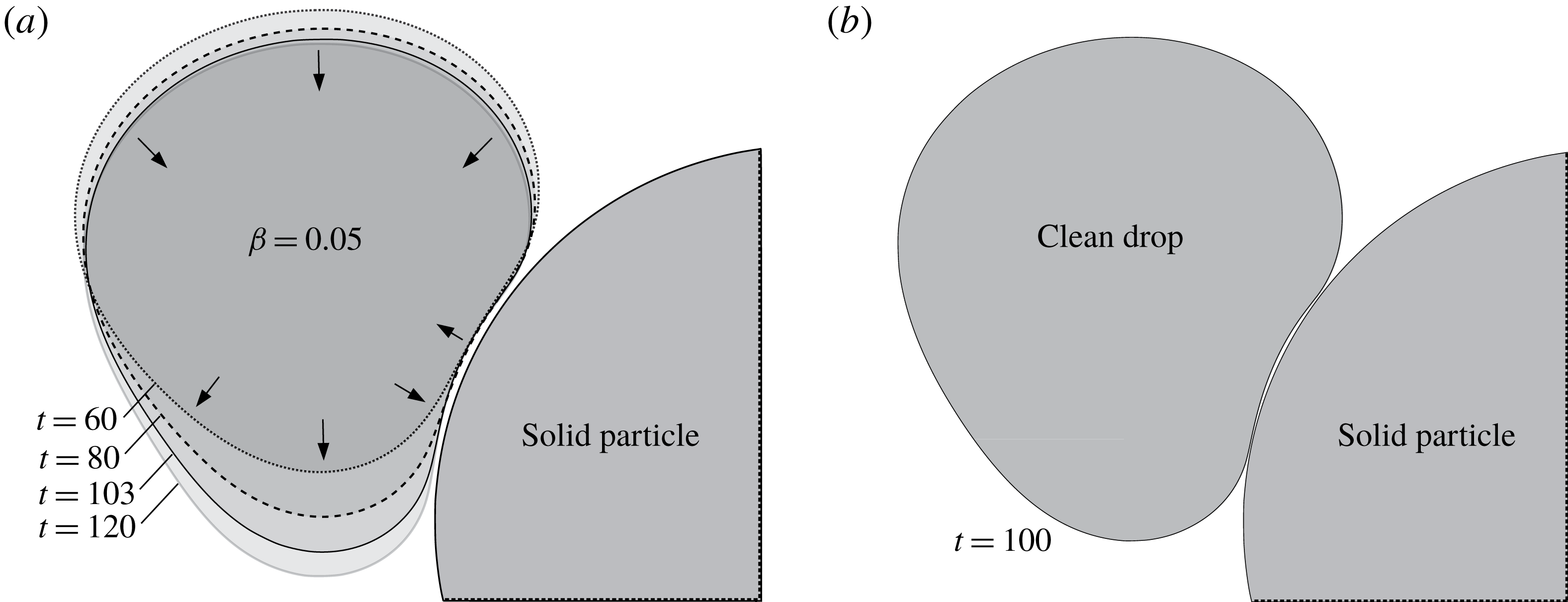
, a significant portion of the drop, including the majority of highly concentrated surfactant, may extend past the centre of the constriction and remain in a stable trapped state (figure 9). A contaminated trapped drop, according to mass balance, should become immobilized at steady state in regions with non-uniform surfactant concentrations. The effect of low contamination on steady-state interfacial velocities is shown in figure 10. Due to the use of higher-order singularity subtraction in the boundary-integral algorithm, drop velocity can stably decrease by more than four orders of magnitude, at which point a drop is assumed to be in a trapped state. The effect of contamination on surface velocity becomes transparent when viewed with a logarithmic scale: regions containing surfactant show a marked decrease in velocity, including the development of a ‘stagnant cap’ on the downwind pole. Additionally, surfactant modifies the overall flow field. Rather than divergent interfacial velocity at the approximate centre of the dimple as is characteristic of clean drops, the entirety of the dimple region develops a flow that is opposite to the far-field direction, and elongated vortices develop along its edges (figure 10). The effect of this modified surface velocity field on the minimum drop–solid separation is weak, with the gap between
 ${\sim}0.011$
and 0.012 in both cases, at steady state. However, in the contaminated system, the thickness of the lubrication layer is more uniform, as discussed in § 5.4.
Surfactant contamination tends to decrease the interfacial velocity magnitude (
 $u_{s}$
) of steady-state trapped drops (
 $\unicode[STIX]{x1D706}=4.0$
,
 $\widetilde{N}_{\triangle }=20~\text{K}$
,
 $\widehat{N}_{\triangle }=11.5~\text{K}$
). Velocities are binned using colours according to a logarithmic scale. Large arrows indicate the general shape of the velocity field, which is affected by contamination. Drop is rotated to show dimpled face; solid particles not shown.

5.3 Viscosity ratio
Low viscosity ratios,
 $\unicode[STIX]{x1D706}\sim 0.1$
or less, pose a significant hurdle for numerical treatment of convection-dominated surfactant transport in complex flow fields. Single drops in simple shear flow have been reported to demonstrate unphysical negative surface tension within relevant parameter ranges, regardless of the governing equation of state (Bazhlekov et al.
Reference Bazhlekov, Anderson and Meijer2006). A similar issue is encountered for tight squeezing when using prior LS or FV convection schemes, regardless of whether implicit, explicit or semi-implicit time integration is used to advance surfactant concentrations. Visualizing the simulation at every time step up to failure reveals that it is typically a single node near high concentration gradients that receives an erroneously high amount of surfactant. Advection of non-diffusive scalar fields, e.g. within flows that may include sharp density gradients or shock waves, is common in inviscid fluid flow modelling. It is standard to convect such fields with an upwind scheme, an integration technique that is biased toward velocities upstream of the control volume and exhibits increased numerical stability. The only convection methods tested in this study that were stable for tight squeezing of low-viscosity-ratio drops are the first-order upwind FV and FBLS schemes for unstructured meshes. For all runs that showed no signs of unphysical behaviour, regardless of the convection method used, the minimum value of surface tension (
 $\unicode[STIX]{x1D70E}_{min}$
) remained above
 $\unicode[STIX]{x1D70E}_{min}\gtrsim 0.5$
. Therefore, Marangoni stresses appear sufficient to prevent the development of unphysical negative surface tension in these systems even when coupled to a linear equation of state.
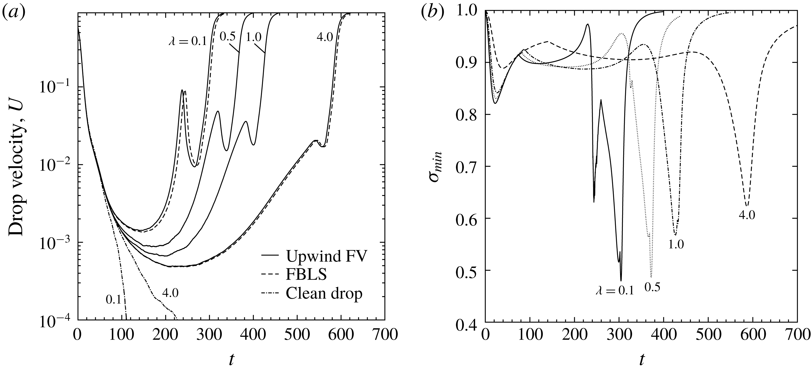
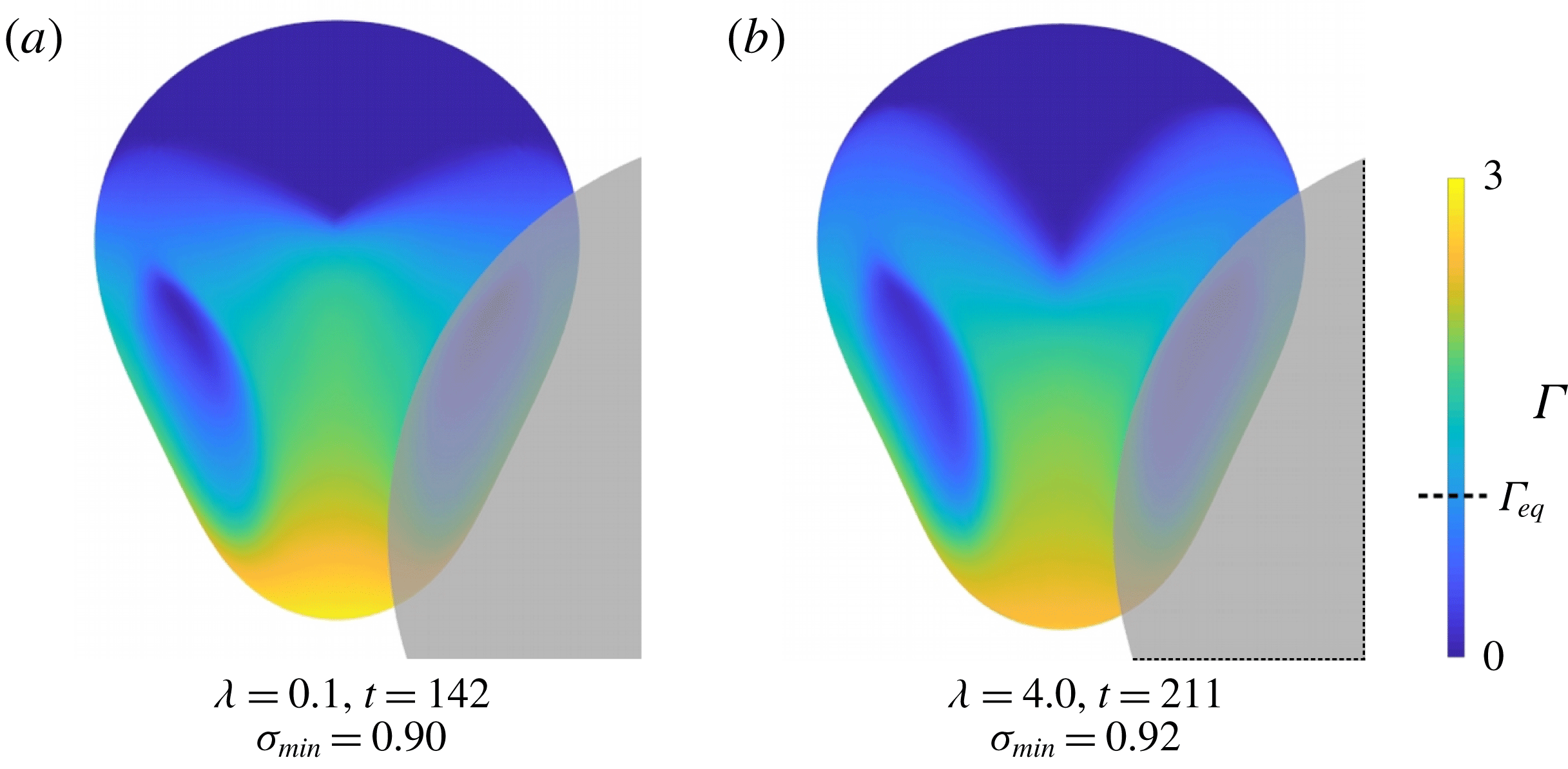
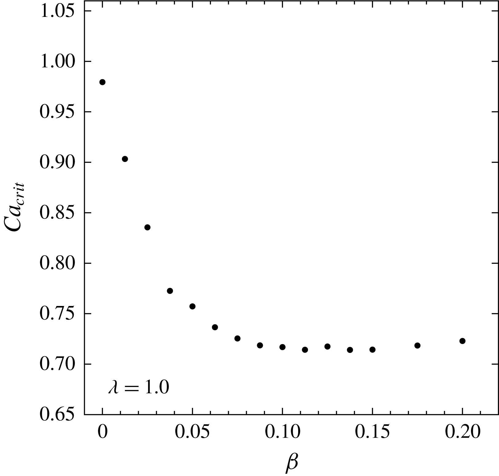
As shown in figure 11(a), the dependence of contaminated-drop squeezing dynamics on viscosity ratio follows a trend similar to that of clean drops at supercritical capillary numbers (Zinchenko & Davis Reference Zinchenko and Davis2006). However, the evolution of surfactant becomes steadily more complex, as seen in figure 11(b), due to its ability to more quickly respond to the transient stress field at the interface. Recall that discontinuities in the derivative of
 $\unicode[STIX]{x1D70E}_{min}$
generally correspond to a change in the locale of maximum surfactant concentration. For example, additional cusps in
 $\unicode[STIX]{x1D70E}_{min}$
versus time appear for lower
 $\unicode[STIX]{x1D706}$
, approximately when the drop is halfway through the constriction (see figure 11
b:
 $\unicode[STIX]{x1D706}=0.1$
,
 $t\approx 250$
). Visualizing the evolution of surfactant at this time reveals that the high surfactant concentration at the leading tip is briefly transported away, back toward and through the centre of the constriction, presumably driven by Marangoni stresses (figure 12). This effect ultimately results in the drop exiting the constriction with a bimodal distribution of surfactant, having high concentrations at both the leading and trailing poles of the drop, in contrast to just the downwind pole as observed with higher viscosity ratios (figure 5).
Dependence of contaminated-drop squeezing dynamics on viscosity ratio (
 $Ca=0.9$
,
 $\unicode[STIX]{x1D6FD}=0.05$
,
 $\widetilde{N}_{\triangle }=20~\text{K}$
,
 $\widehat{N}_{\triangle }=8.6~\text{K}$
). (a) Monotonically decreasing squeezing times with decreasing viscosity ratio. Subcritical clean drop (
 $\unicode[STIX]{x1D6FD}=0$
) behaviour shown for comparison. (b) Surfactant distributions undergo greater variation at low viscosity ratios.

Mechanism by which a drop at low viscosity ratio can exit a three-sphere constriction with a nearly symmetric bimodal surfactant distribution (
 $Ca=0.9$
,
 $\unicode[STIX]{x1D6FD}=0.05$
,
 $\unicode[STIX]{x1D706}=0.1$
,
 $\widetilde{N}_{\triangle }=15.4~\text{K}$
,
 $\widehat{N}_{\triangle }=11.5~\text{K}$
). During a relatively short duration while the drop is approximately centred with respect to the spherical particles, surfactant concentration is drawn upward through the constriction. At each time step, the colourbar is rescaled with respect to the maximum gamma concentration.

Transient surfactant distributions for
 $\unicode[STIX]{x1D706}=0.1$
and
 $\unicode[STIX]{x1D706}=4.0$
are shown in figure 13, at the time of global drop velocity minimum (
 $U_{min}$
) of their respective squeezing trajectories. Surfactant-concentration extrema tend to be amplified by lower viscosity ratios, at analogous stages in the squeezing process. At
 $U_{min}$
, the inner constriction flow field has swept significant amounts of surfactant to the downstream pole, reaching
 $\unicode[STIX]{x1D6E4}_{max}=2.9$
for
 $\unicode[STIX]{x1D706}=0.1$
and
 $\unicode[STIX]{x1D6E4}_{max}=2.6$
for
 $\unicode[STIX]{x1D706}=4.0$
. Sharper surfactant gradients are observed for
 $\unicode[STIX]{x1D706}=0.1$
, particularly at the ‘triple point’ upstream from particle interstices. This point is typically where numerical difficulties arise with convection methods other than the flow-biased schemes. Also, Marangoni stresses become strong enough to partially refill depleted dimple regions, which begin with relatively uniform near-zero concentrations at the onset of squeezing, to a greater extent at low viscosity ratios.
Effect of viscosity ratio on surfactant distribution (
 $Ca=0.9$
,
 $\unicode[STIX]{x1D6FD}=0.05$
) at analogous points in the squeezing process (
 $U_{min}$
). One of the three solid spheres comprising the constriction is shown for reference, rendered in translucent grey. (a) Low viscosity ratio results in higher maximum concentrations (
 $\unicode[STIX]{x1D70E}_{min}=0.90~\widehat{=}\unicode[STIX]{x1D6E4}_{max}=2.9$
) and steeper gradients. (b) Analogous snapshot of surfactant distribution for high viscosity ratio and moderately supercritical
 $Ca$
(
 $\unicode[STIX]{x1D70E}_{min}=0.92~\widehat{=}~\unicode[STIX]{x1D6E4}_{max}=2.6$
).

5.4 Degree of contamination
The degree of surfactant contamination, quantified by the elasticity parameter (
 $\unicode[STIX]{x1D6FD}$
), is most influential on squeezing dynamics at near-critical capillary numbers or low viscosity ratios. For example, no appreciable difference in squeezing times is observed between
 $\unicode[STIX]{x1D6FD}=0.05$
and
 $\unicode[STIX]{x1D6FD}=0.2$
at high capillary number and viscosity ratios (
 $Ca=1.3,\unicode[STIX]{x1D706}=4.0$
). However, at
 $Ca=0.85$
, increasing from low (
 $\unicode[STIX]{x1D6FD}=0.05$
) to medium (
 $\unicode[STIX]{x1D6FD}=0.1$
) degrees of contamination considerably decreases squeezing times (figure 14
a). For
 $\unicode[STIX]{x1D6FD}\leqslant 0.1$
,
 $T_{s}$
obeys the power-law relation provided in figure 14(b). Extrapolating to a trapped state (
 $T_{s}\rightarrow \infty$
) would imply that
 $\unicode[STIX]{x1D6FD}_{crit}=0.03$
for this system. For
 $\unicode[STIX]{x1D6FD}$
above a maximum value, further increases in degree of contamination have a negligible effect on squeezing times (figure 14
b). This effect could be of interest, e.g. to the field of enhanced oil recovery, for which diminishing returns are observed when surfactant levels are raised above a certain value.
Effect of elasticity parameter (degree of contamination) on squeezing dynamics (
 $Ca=0.85,\unicode[STIX]{x1D706}=4.0$
,
 $\widetilde{N}_{\triangle }=20~\text{K}$
,
 $\widehat{N}_{\triangle }=8.6~\text{K}$
). (a) Degree of contamination has an appreciable effect on squeezing times at near-critical conditions. (b) Elasticity parameter versus squeezing times exhibits a power-law fit below a maximum value (solid circles), above which increasing
 $\unicode[STIX]{x1D6FD}$
has negligible effect on
 $T_{s}$
. Outlying (unfitted) data points denoted by
 $\times$
marks.

The same trend is observed for low viscosity ratios (
 $\unicode[STIX]{x1D706}=0.1$
). As seen in figure 15(a,b), squeezing times remain almost constant for
 $\unicode[STIX]{x1D6FD}\geqslant 0.1$
. To isolate the mechanism for this behaviour, we searched for other system parameters that follow a similar trend with respect to
 $\unicode[STIX]{x1D6FD}$
. The minimum gap between drop and particle during early drop squeezing is shown in figure 15(c). During initial droplet approach, there is a clear trend of smaller separation with decreasing contamination, which can be attributed to surfactant’s effect on the lubrication layer, as discussed below. However, because this initial gap disparity quickly converges, it is not expected to influence overall squeezing times. As observed for capillary number, there is a very weak dependence of gap on degree of contamination for the majority of the squeezing process, being essentially independent after
 $t\geqslant 100$
. A metric for the evolution of the surfactant concentration is shown in figure 15(d). To directly compare surfactant concentration versus degree of contamination, concentration is scaled by
 $\unicode[STIX]{x1D6FD}$
and shifted according to its initial value. The metric
 $\unicode[STIX]{x0394}(\unicode[STIX]{x1D6FD}\unicode[STIX]{x1D6E4}_{max})=\unicode[STIX]{x1D6FD}\unicode[STIX]{x1D6E4}_{max}-(\unicode[STIX]{x1D6FD}\unicode[STIX]{x1D6E4}_{max})_{eq}$
represents the relative increase in surfactant concentration. This metric appears to be converging at local extrema, for example at
 $t\approx 20$
, with respect to increasing
 $\unicode[STIX]{x1D6FD}$
. Recall that the first local minimum of
 $\unicode[STIX]{x1D6E4}_{max}$
(
 $t\approx 65$
) represents the shift in location of
 $\unicode[STIX]{x1D6E4}_{max}$
from the drop equator to the leading tip of the drop (see the inset of figure 15
d). A clear trend is the gradual decrease in the right derivative of
 $\unicode[STIX]{x1D6E4}_{max}$
at the cusp, indicating that at low viscosity ratios and high degrees of contamination, Marangoni stresses almost immediately begin to draw surfactant away from the leading tip as it begins to pass through the constriction.
Effect of elasticity parameter on squeezing dynamics at low viscosity ratio (
 $Ca=0.9,\unicode[STIX]{x1D706}=0.1,\widetilde{N}_{\triangle }=15.4~\text{K},\widehat{N}_{\triangle }=11.5~\text{K}$
). (a) Drop dynamics for a range of degree of contamination. (b) Power-law fitting of squeezing times. Outlying (unfitted) data points denoted by
 $\times$
marks. (c) Drop–particle gap is sensitive to contamination for
 $t<100$
. (d) Evolution of surfactant concentration with respect to contamination. For direct comparison,
 $\unicode[STIX]{x1D6E4}_{max}$
is scaled by
 $\unicode[STIX]{x1D6FD}$
and shifted by
 $(\unicode[STIX]{x1D6FD}\unicode[STIX]{x1D6E4}_{max})_{eq}$
. for super- and subcritical
 $Ca$
. Inset: shift of
 $\unicode[STIX]{x1D6E4}_{max}$
to the leading tip of the drop.

Average surface mobility continues to decrease with increasing contamination, for the majority of the squeezing process, as shown in figure 16(a). This trend also indicates the continued increase in the strength of Marangoni stresses with respect to hydrodynamic stresses. The distribution of surfactant and surface flow field are also significantly affected by increasing contamination. Surface velocities for various
 $\unicode[STIX]{x1D6FD}$
values are shown in figure 16(b), at respective global minima of drop velocity. The distribution of surface velocities also indicates key regions of surfactant distribution; e.g. the surface extensional flow indicated by arrows corresponds to the sharp surfactant gradient universally observed on the top surface. With increasing contamination, this sharp gradient nears the top pole of the drop, to the point of almost vanishing for
 $\unicode[STIX]{x1D6FD}=0.15$
. The disappearance of this near-zero concentration region, along with a similar filling of surfactant into near-contact regions, results in almost the entire drop surface hosting a significant amount of surfactant. The presence of surfactant generally results in dramatically decreased tangential velocity, as is visually apparent by the receding region of
 $u_{s}>10^{-2}$
on the top surface.
Effect of degree of contamination on interface mobility (
 $Ca=0.9$
,
 $\unicode[STIX]{x1D706}=0.1$
,
 $\widetilde{N}_{\triangle }=15.4~\text{K}$
,
 $\widehat{N}_{\triangle }=11.5~\text{K}$
). (a) Surface mobility steadily decreases with increasing contamination. (b) Distribution of tangential velocity, binned on a logarithmic scale, for various
 $\unicode[STIX]{x1D6FD}$
at respective global minima of squeezing velocity. The location of surface extensional flow, indicative of a sharp surfactant-concentration gradient, is highlighted with arrows. Drop is rotated to show dimpled face; solid particles not shown.

To examine the effect of degree of contamination on droplet trapping, a systematic study of critical capillary number was completed at unit viscosity ratio, shown in figure 17. As was noted for
 $\unicode[STIX]{x1D706}=4$
, a dramatic reduction of
 $Ca_{crit}$
is observed between clean drops (
 $\unicode[STIX]{x1D6FD}=0$
) and
 $\unicode[STIX]{x1D6FD}=0.05$
, decreasing by
 $25\,\%$
in this case (
 $\unicode[STIX]{x1D706}=1$
). The intervening data reveal that the dependence is nearly linear within this range of
 $\unicode[STIX]{x1D6FD}$
values. Above
 $\unicode[STIX]{x1D6FD}\approx 0.1$
,
 $Ca_{crit}$
remains almost constant, indicating a minimum degree of contamination in order to maximize droplet pass-through, e.g. when capillary number is uncertain. Similar to the effect of
 $\unicode[STIX]{x1D6FD}$
on squeezing times at fixed
 $Ca$
, the lack of dependence of
 $Ca_{crit}$
on degree on contamination above a certain
 $\unicode[STIX]{x1D6FD}$
value is attributed to tangential immobilization of the interface.
Effect of degree of contamination on critical capillary number at unit viscosity ratio (
 $\widetilde{N}_{\triangle }=15.4~\text{K}$
,
 $\widehat{N}_{\triangle }=11.5~\text{K}$
). Each
 $Ca_{crit}$
is extrapolated from supercritical squeezing times using a power-law regression.
 $Ca_{crit}$
decreases linearly when
 $\unicode[STIX]{x1D6FD}\leqslant 0.04$
, and remains almost constant above
 $\unicode[STIX]{x1D6FD}\approx 0.1$
.

Cutaway of droplet squeezing through the three-sphere constriction, showing the lubrication layer (
 $Ca=0.9$
,
 $\unicode[STIX]{x1D706}=0.1$
,
 $\widetilde{N}_{\triangle }=15.4~\text{K}$
,
 $\widehat{N}_{\triangle }=11.5~\text{K}$
). Planar cross-section passes through the centre of the constriction and one particle. (a) Contaminated-drop squeezing (
 $\unicode[STIX]{x1D6FD}=0.05$
). Arrows indicate the general direction of interfacial movement. The expanding drop tip is observed to most closely approach the surface of the particle. (b) Snapshot of clean-drop planar cross-section at the same capillary number and viscosity ratio (
 $\widetilde{N}_{\triangle }=20~\text{K}$
,
 $\widehat{N}_{\triangle }=20~\text{K}$
).

Finally, we consider the effect of contamination on the lubrication layer. As mentioned above, increasing
 $\unicode[STIX]{x1D6FD}$
has negligible effect on the minimum drop–particle separation for
 $t>100$
, but tends to result in a larger gap during early stages of drop squeezing. An interesting aspect of the gap evolution is the appearance of two cusps in gap versus time, especially at low viscosity ratio and low contamination (figure 15
c). For
 $\unicode[STIX]{x1D6FD}=0.05$
, these singularities occur at
 $t\approx 80$
and
 $t\approx 103$
, with the drop–particle gap converging with other
 $\unicode[STIX]{x1D6FD}$
values at the second point. To view the lubrication layer during these times, we consider a planar cross-section of the system, passing through the constriction and particle centres, as shown in figure 18(a). Interestingly, especially for
 $t\leqslant 80$
, the lubrication layer is quite uniform; in contrast, for clean drops a more pronounced dimple is observed, even after accounting for the curvature of the spherical surface (see figure 18
b). The transition between
 $t=103$
and
 $t=120$
reveals that it is the leading tip of the drop that most closely approaches the solid particle, notably breaking the uniformity of the lubrication layer. The expansion of the drop tip toward the particle surface is responsible for the monotonic decrease of drop–solid separation, and this gap is independent of degree of contamination.
6 Concluding remarks
The behaviour of tight-squeezing drops contaminated with insoluble surfactant was investigated using high-resolution 3D boundary-integral simulations. The drops are freely suspended in a uniform far-field flow, and the constriction is composed of three solid particles fixed in space. Drops are initially spherical with a uniform surfactant distribution, and a linear equation of state relates surfactant concentration to surface tension. Stable modelling of near-critical capillary numbers and trapped states is enabled by the desingularization techniques developed by Zinchenko & Davis (Reference Zinchenko and Davis2006, Reference Zinchenko and Davis2017a
). The boundary-integral formulation precisely resolves the fluid–fluid interface, allowing for the straightforward implementation of several distinct convection schemes for surfactant transport. Upwind-biased schemes were found to be the most stable and were required to model tight squeezing for certain parameter ranges of interest, such as low viscosity ratios (
 $\unicode[STIX]{x1D706}\lesssim 0.25$
). Drop squeezing is characterized with respect to capillary number, viscosity ratio and degree of contamination,
 $\unicode[STIX]{x1D6FD}$
.
The evolution of surfactant on the drop surface is visually similar for all parameter ranges of interest. A characteristic aspect of contaminated tight squeezing is the development of sharp surfactant-concentration gradients. These gradients develop quickly at the onset of squeezing due to the competition between advection of the interface and resistive Marangoni stresses. Due to the compressional flow upstream from a constriction, surfactant concentrates around the drop equator, in particular at regions above solid-particle interstices. During the development of a typical trapped-drop shape, the top surface and near-contact regions are host to almost zero surfactant, especially at low degrees of contamination. Surfactant is gradually swept to the leading tip of the drop, decreasing local surface tension and allowing passage through the constriction, and the remainder of the drop quickly follows. Although the evolution of drop shapes resembles that of tight-squeezing clean drops, contamination and the resulting variable local surface tension significantly affects squeezing dynamics.
The addition of small amounts of surfactant decreases the critical capillary number and modifies the interfacial velocity field. A small degree of contamination,
 $\unicode[STIX]{x1D6FD}=0.05$
, is found to decrease the critical capillary number for squeezing
 $Ca_{crit}$
from
 ${\sim}1$
to
 ${\sim}0.8$
for
 $\unicode[STIX]{x1D706}=4.0$
. The mechanism of near-critical contaminated-drop squeezing can be summarized by three stages: development of a typical trapped state, surfactant accumulation at the downwind pole and subsequent elongation of the drop tip. The interfacial flow field is also significantly modified by the presence of surfactant. The tangential surface velocity is decreased in regions of non-zero surfactant, particularly at the leading tip. For a clean drop, a divergent surface velocity is observed at the approximate centre of the drop dimple. For contaminated drops, the entirety of the near-contact region has an interfacial velocity in a direction opposite to that of the far-field flow. For a trapped drop at
 $\unicode[STIX]{x1D706}=4.0$
, resistance from Marangoni stresses governed by a linear equation of state are sufficient to keep local surfactant concentrations within
 ${\sim}3$
times the equilibrium value.
The influence of surfactant is most prominent at low viscosity ratios. Extremely sharp surfactant gradients develop even within the compressional flow upstream from the constriction. The surfactant distribution more quickly responds to the transient stress field, enhancing the ability of Marangoni stresses to partially refill surfactant-depleted near-contact regions. During the later stages of squeezing, this increased responsiveness allows surfactant accumulated at the leading tip to be ‘pulled’ back through the constriction, resulting in a bimodal distribution at exit. Although the evolution of surfactant becomes more complex at low viscosity ratios, squeezing times as a function of viscosity ratio follow a similar trend to that of clean drops. Even at the low viscosity ratio
 $\unicode[STIX]{x1D706}=0.1$
and moderately supercritical conditions (
 $Ca=0.9,\unicode[STIX]{x1D6FD}=0.05$
), Marangoni stresses governed by a linear equation of state are sufficient to retain positive values of surface tension. During the early and middle stages of tight squeezing, which is most representative of squeezing through large-scale granular media,
 $\unicode[STIX]{x1D70E}$
remains within 20 % of
 $\unicode[STIX]{x1D70E}_{eq}$
.
Critical capillary number and drop squeezing time decrease with increasing degree of contamination, up to a certain saturation
 $\unicode[STIX]{x1D6FD}$
-value above which increasing
 $\unicode[STIX]{x1D6FD}$
has negligible effect. For unit viscosity ratio, the maximum decrease in
 $Ca_{crit}$
due to contamination is as much as 27 %. In all cases, this saturation occurs at
 $\unicode[STIX]{x1D6FD}\approx 0.1$
. The phenomenon of diminishing returns with respect to increasing surfactant may be of interest e.g. to the field of enhanced oil recovery. The trend is characterized by the increasing strength of Marangoni stresses, which effectively limit the maximum surfactant concentration. In addition, for highly contaminated surfaces, the surface area of near-zero surfactant regions decreases considerably, resulting in the disappearance of sharp concentration gradients and the steady decrease of average surface mobility. It is concluded that surfactants have a significant impact on the hydrodynamics of fluid–fluid interfaces under tight-squeezing conditions, generally increasing the ease with which drops can pass through tight constrictions.
On the methodological side, an essential finding of the present work is in understanding the origin of the negative surface tensions sometimes observed in prior simulations for concentrated contaminated emulsions in the limit of non-diffusive surfactant (Zinchenko & Davis Reference Zinchenko and Davis2017a ). This artifact happens to arise from numerical instability of prior surfactant transport schemes and is not a physical deficiency of the linear equation of state for surfactant. The upwind finite-volume (FV) and substantially new flow-biased least-squares (FBLS) schemes implemented herein resolve this issue, at least for drop-squeezing simulations. As a general tool for surfactant transport on a deformable surface, our upwind FV implementation is probably most stable, although it comes with resolution-dependent numerical diffusion (somewhat larger than for FBLS). Close agreement between the results by these two, very different schemes demonstrates that the limit of non-diffusive surfactant is nevertheless achieved in the present simulations.
Work is in progress to extend the present study to large-scale simulations of contaminated-emulsion flow through porous media. A successful implementation for many clean drops driven through a randomly packed bed under a pressure gradient was recently achieved by Zinchenko & Davis (Reference Zinchenko and Davis2013) with multipole acceleration, including treatment of cascading drop breakup. Replicating such a system with surfactant-laden drops requires an extremely robust algorithm for surfactant transport, due to the diversity of solid–drop and drop–drop interactions in complex environments. Care was taken in the present work to achieve universal stability at near-critical capillary numbers and low viscosity ratios. It is expected that, just as for the present single-drop system, the presence of surfactant will significantly modify the macroscale emulsion properties. For example, during primary drop breakup, it can be expected that the resultant fragments have notably different equilibrium surface tensions due to non-uniform surfactant distribution at breakup (Kovalchuk et al. Reference Kovalchuk, Jenkinson, Miller and Simmons2018). Efforts are also underway to incorporate nonlinear equations of state and complex-shaped particles. For the latter, we expect squeezing between parallel oblong particles to be more difficult than the current three-sphere constriction, due to the absence of interparticle interstices. Sharp corners, such as in a planar constriction, will present difficulties from drop–corner contact due to lack of lubrication and will require corner smoothing.
Acknowledgements
This work utilized, in part, the RMACC Summit supercomputer, which is supported by the National Science Foundation (awards ACI-1532235 and ACI-1532236), the University of Colorado Boulder, and Colorado State University. The Summit supercomputer is a joint effort of the University of Colorado Boulder and Colorado State University.