


1 Introduction
Ultra-short laser pulses are critical to many applications ranging from next-generation medical technologies[ Reference Glinec, Faure, Malka, Fuchs, Szymanowski and Oelfke 1 ], to non-destructive material testing[ Reference Glinec, Faure, Dain, Darbon, Hosokai, Santos, Lefebvre, Rousseau, Burgy, Mercier and Malka 2 ] and to next-generation particle acceleration[ Reference Tajima and Dawson 3 ], to list a few. Since the invention of chirped-pulse amplification (CPA)[ Reference Strickland and Mourou 4 ], femtosecond, multi-terawatt systems have proliferated, enabling the exploration of extreme light–matter interactions[ Reference Mourou, Tajima and Bulanov 5 ]. These laser pulses have significant spectral bandwidths and have large apertures in the near-field. These characteristics together enable the emergence of spatially nonuniform pulse-front delays and pulse durations from dispersion effects accumulated throughout the beam path[ Reference Akturk, Gu, Bowlan and Trebino 6 ]. These spatially dependent chromatic distortions, known as spatio-temporal couplings (STCs), have been found to be caused by numerous components throughout the laser generation, amplification and beam transport, and by imperfect compensation of the STCs introduced in the stretcher–compressor CPA setups, and have been detected in a wide array of systems[ Reference Jeandet, Jolly, Borot, Bussière, Dumont, Gautier, Gobert, Goddet, Gonsalves, Irman, Leemans, Lopez-Martens, Mennerat, Nakamura, Ouillé, Pariente, Pittman, Püschel, Sanson, Sylla, Thaury, Zeil and Quéré 7 ].
Accurate spatio-temporal or spatio-spectral metrology and control is of great importance to the effective use of such laser systems[ Reference Walmsley and Dorrer 8 ]. In typical experimental setups, the goal is to avoid undesirable STCs, which can decrease intensity at focus and distort the quality of the beam[ Reference Akturk, Gu, Bowlan and Trebino 6 ]. Recently, advanced schemes have been suggested for utilizing spatio-temporal manipulation of the beam[ Reference Piccardo, Cernaianu, Palastro, Arefiev, Thaury, Vieira, Froula and Malka 9 ]. These include combining STCs with specialized optics that allow for an extended focus that propagates at a tunable velocity. The tunability of such flying-focus pulses has been experimentally demonstrated using several configurations[ Reference Sainte-Marie, Gobert and Quere 10 – Reference Pigeon, Franke, Chong, Katz, Boni, Dorrer, Palastro and Froula 12 ] and shows promise in achieving higher energy particle acceleration[ Reference Debus, Pausch, Huebl, Steiniger, Widera, Cowan, Schramm and Bussmann 13 – Reference Liberman, Golovanov, Tata, Talposi and Malka 18 ], more efficient terahertz generation[ Reference Simpson, Pigeon, Miller, Ramsey, Froula and Palastro 19 ] and laser-wakefield acceleration of ions[ Reference Gong, Cao, Palastro and Edwards 20 ], and enabling laser-based undulators for X-ray free electron lasers[ Reference Ramsey, Malaca, Simpson, Formanek, Mack, Vieira, Froula and Palastro 21 ]. Another use that has generated significant interest is the generation of vortex beams[ Reference Sueda, Miyaji, Miyanaga and Nakatsuka 22 , Reference Shi, Zhang, Arefiev and Shen 23 ], which have shown promise in both electron acceleration[ Reference Blackman, Shi, Klein, Cernaianu, Doria, Ghenuche and Arefiev 24 ] and proton acceleration[ Reference Willim, Vieira, Malka and Silva 25 ] and have been adapted to large-aperture, high-intensity beams[ Reference Iancu, Talpoşi, Gheorghiu, Ungureanu, Dăncuş, Matei and Ursescu 26 ].
A number of spatio-spectral and spatio-temporal metrology methods have been developed[ Reference Akturk, Gu, Bowlan and Trebino 6 , Reference Dorrer 27 , Reference Jolly, Gobert and Quéré 28 ]. Several are based on the use of spatially resolved Fourier transform spectrometry (SRFTS)[ Reference Miranda, Kotur, Rudawski, Guo, Harth, L’Huillier and Arnold 29 , Reference Pariente, Gallet, Borot, Gobert and Quere 30 ], using a spatially filtered self-reference pulse. Perhaps the most widely used measurement method, INSIGHT[ Reference Borot and Quere 31 ], is based on a similar scanning interferometric setup, but the measurement is conducted at focus rather than in the near-field, and the Gerchberg–Saxton (GS) iterative algorithm[ Reference Gerchberg 32 ] is used to reconstruct the spectrally resolved spatial profile of the beam. Other methods rely on spatially resolved spectral interferometry[ Reference Alonso, Sola, Varela, Hernández-Toro, Méndez, Román, Zaïr and Roso 33 ], wavelength-resolved wavefront measurement techniques[ Reference Cousin, Bueno, Forget, Austin and Biegert 34 ], digital holography[ Reference Gabolde and Trebino 35 ], optical filtering of the measured pulse[ Reference Weiße, Esslinger, Howard, Foerster, Haberstroh, Doyle, Norreys, Schreiber, Karsch and Döpp 36 ], broadband Young’s double slit interferometry[ Reference Smartsev, Tata, Liberman, Adelberg, Mohanty, Levine, Seemann, Wan, Kroupp, Lahaye, Thaury and Malka 37 ] and hyperspectral imaging[ Reference Batey, Claus and Rodenburg 38 ]. Some techniques use imaging spectrometers to measure the pulse, but this is limited to one dimension[ Reference Witting, Frank, Arrell, Okell, Marangos and Tisch 39 ] rather than fully measuring the pulse. Lately, a number of one-shot techniques have emerged, promising shot-to-shot measurement of the pulse[ Reference Tang, Men, Liu, Hu, Su, Zuo, Li, Liang, Downer and Li 40 – Reference Kim, Kim, Yoon, Sung, Lee and Nam 43 ]. These include IMPALA[ Reference Smartsev, Liberman, Andriyash, Cavagna, Flacco, Giaccaglia, Kaur, Monzac, Tata, Vernier, Malka, Lopez-Martens and Faure 41 ], which algorithmically separates out spectral information in the Fourier plane, allowing for multiple GS algorithms to be run for different colors.
In recent years, a number of systems have emerged that provide few-cycle pulses with durations at or below 10 fs and with peak powers in the terawatt scale, such as the Salle Noire laser at Laboratoire d’Optique Appliqué[ Reference Guénot, Gustas, Vernier, Beaurepaire, Böhle, Bocoum, Lozano, Jullien, Lopez-Martens, Lifschitz and Faure 44 ], the PFS laser system at Ludwig-Maximilians-Universität München[ Reference Nubbemeyer, Kaumanns, Ueffing, Gorjan, Alismail, Fattahi, Brons, Pronin, Barros, Major, Metzger, Sutter and Krausz 45 ], the LUCID laser system at the Lund Laser Centre (LLC)[ Reference Balciunas, Juodagalvis, Girdauskas, Budriunas, Maslinskas and Stanislauskas 46 ] and a number of facilities inside the ELI-ALPS facility[ Reference Budriūnas, Stanislauskas, Adamonis, Aleknavičius, Veitas, Gadonas, Balickas, Michailovas and Varanavičius 47 ]. Some of these laser systems rely on novel laser architectures[ Reference Nubbemeyer, Kaumanns, Ueffing, Gorjan, Alismail, Fattahi, Brons, Pronin, Barros, Major, Metzger, Sutter and Krausz 45 – Reference Budriūnas, Stanislauskas, Adamonis, Aleknavičius, Veitas, Gadonas, Balickas, Michailovas and Varanavičius 47 ], while others utilize advances in spectral broadening and post-compression technology[ Reference Mironov, Lozhkarev, Khazanov and Mourou 48 , Reference Wheeler, Bleotu, Naziru, Fabbri, Masruri, Secareanu, Farinella, Cojocaru, Ungureanu, Baynard, Demailly, Pittman, Dabu, Dancus, Ursescu, Ros, Tajima and Mourou 49 ]. These near-single cycle pulses offer advantages such as particle acceleration with small, relatively low-power systems and unprecedented repetition rates[ Reference Guénot, Gustas, Vernier, Beaurepaire, Böhle, Bocoum, Lozano, Jullien, Lopez-Martens, Lifschitz and Faure 44 ] and the possibility of accelerator optimization with carrier-envelope phase (CEP) control[ Reference Monzac, Smartsev, Huijts, Rovige, Andriyash, Vernier, Tomkus, Girdauskas, Raciukaitis, Mackevičiūtė, Stankevic, Cavagna, Kaur, Kalouguine, Lopez-Martens and Faure 50 , Reference Angella, Löfquist, Gustafsson, Poulain, D’Souza, Guo, Persson, Eng-Johnsson, Wahlström and Lundh 51 ].
Since these pulses have spectral bandwidths of 100 nm or more, they present a significant challenge for existing spatio-spectral and spatio-temporal measurement methods. While many metrology methods can, theoretically, cope with such bandwidths, in practice they rely on conventional complementary metal–oxide–semiconductor (CMOS) sensors and other optical elements, which have greatly varying sensitivity over the bandwidth and a small dynamic range for the LUCID laser (700–1000 nm). Although reasonably priced cameras often offer a nominal dynamic range of up to 16 bits, the effective dynamic range is limited by the sensor noise floor. A substantial portion of the available range is occupied by the high-intensity spectral components. Since the spectral information is reconstructed from the recorded images using a Fourier transform, the low-intensity spectral components become problematic: their signal levels are often comparable to the sensor noise and are further degraded by spatial modulations originating from the high-intensity portions of the spectrum. This, coupled with the fact that the pulses themselves often have strongly nonuniform spectra, means that in many cases parts of the pulse are not being reconstructed properly. Upgrading to indium gallium arsenide (InGaAs) sensors can increase the sensitivity (such as in Ref. [Reference Lehotai, Kiss, Miranda, Charrut, Shrestha, Meng, Guirreiro, Romero, Seres, Gilicze, Cormier, Börzsönyi and Nagymihály52]), but greatly increases the cost of the product. While some existing techniques have measured near-single-cycle pulses[ Reference Alonso, Miranda, Sola and Crespo 53 ], they have often been intrusive, difficult to implement setups that are very sensitive to experimental conditions.
In this paper, we present spatio-spectral and spatio-temporal measurements in the LUCID laser system at the LLC, which provides few-cycle, CEP stable pulses. We show that INSIGHT – which is the closest there to an industry standard STC measurement device – fails to properly reconstruct the full bandwidth of the laser pulse, due to significant variance in the signal strength over the bandwidth. However, when the pulse is spectrally filtered and then stitched together, the joint measurement succeeds in enhancing the dynamic range of the INSIGHT measurement. The method proposed here is improving on the dynamic range by introducing adaptive adjustment of the spectral intensity to better reconstruct low-spectral-intensity components in the pulse.
To demonstrate the robustness and applicability of this enhancement, we show that the same spectral filtering succeeds in recovering lost spectral information in the IMPALA measurement technique as well as in SRFTS. This simple, inexpensive addition to existing STC metrology methods makes accurate reconstruction of few-cycle pulses a possibility, a critical step to allowing these state-of-the-art facilities to achieve their full potential.
2 Materials and methods
2.1 LLC laser system and experimental setup
Experiments were carried out using LUCID, the multi-terawatt optical parametric chirped-pulse amplification (OPCPA) laser system at the LLC[ Reference Balčiūnas, Piel, Zürch, Hädrich, Gaida, Tünnermann, Rothhardt and Pupeza 54 ], manufactured by Light Conversion. The system delivers 9 fs pulses (intensity-envelope full width at half maximum (FWHM)) with an energy of 250 mJ (+1%) prior to transport, corresponding to 190 mJ on target, at a central wavelength of 850 nm and a 10 Hz repetition rate.
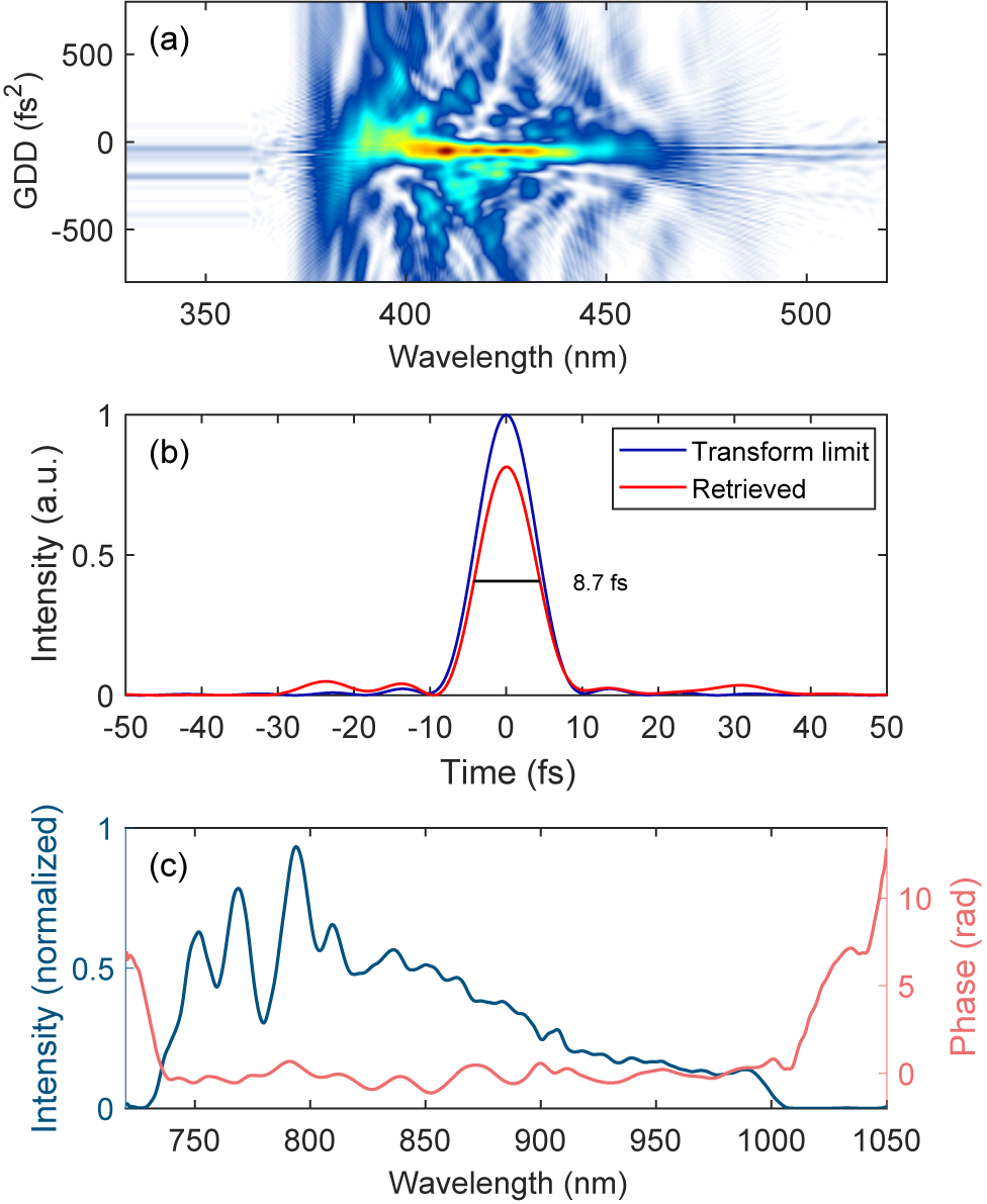
A dispersive scan (d-scan) measurement of the pulse can be seen in Figure 1(a). The d-scan works by inserting known thicknesses of glass into the pulse and capturing the second-harmonic generation spectrum. This results in a two-dimensional (2D) scan that gives information about the spectrum and the spectral phase from which the temporal shape of the pulse can be reconstructed. Figure 1(b) shows the retrieved temporal shape of the pulse, while Figure 1(c) shows the retrieved spectrum and spectral phase. The pulses are compressed in vacuum by means of 16 chirped mirrors with a group delay dispersion (GDD) of 100 fs2 per pair. Aberrations in the spatial profile of the laser can be corrected with an enhanced silver-coated deformable mirror located within the compressor chamber. The short pulse duration of just over three laser cycles corresponds to a very wide spectral bandwidth of almost 300 nm, making this laser system highly susceptible to STCs, whose characterization is therefore of great importance. The laser is CEP stable due to a difference frequency generation (DFG) based front-end, while the phase drift is detected by an f-2f interferometer located upstream of the compressor and feeding back to DAZZLER equipment, yielding a root mean square (RMS) CEP stability of 340 mrad.
Pulse characterization of the LUCID laser. (a) Dispersion scan measurement. (b) Retrieval of the temporal pulse shape. (c) Retrieved spectrum and spectral phase of the laser.

Figure 1. Long description
Panel a is a dispersion scan heat map. The x-axis represents Wavelength in n m from 350 to 500. The y-axis represents G D D in f s squared from minus 500 to 500. A central horizontal yellow and green intensity band is concentrated around 0 G D D between 380 and 450 n m, surrounded by blue interference patterns.
Panel b is a line graph of Intensity in a.u. versus Time in f s from minus 50 to 50. A blue line labeled Transform limit shows a sharp Gaussian peak at 0 f s reaching an intensity of 1. A red line labeled Retrieved shows a slightly lower peak at 0 f s with a measured width of 8.7 f s. Small side lobes are visible between minus 30 and minus 10 f s and 20 to 40 f s.
Panel c is a dual-axis line graph. The x-axis shows Wavelength in n m from 750 to 1050. The left y-axis is Intensity normalized in blue, showing a multi-peaked curve that rises at 750 n m, peaks near 800 n m, and gradually decays to 0 by 1000 n m. The right y-axis is Phase in radians in pink, showing a relatively flat profile near 0 radians between 750 and 1000 n m, with sharp increases at the spectral edges.
The laser’s energy can be attenuated either by lowering the pump energy in the last two off-axis parabola (OPA) stages or by inserting a combination of 4-inch optical density (OD) filters in the beam prior to pulse compression. After the compression stage, all beam transport is in vacuum and utilizes enhanced silver-coated mirrors. All beam transport after compression is in the horizontal plane. The beam has a diameter of 50 mm during the vacuum transport.
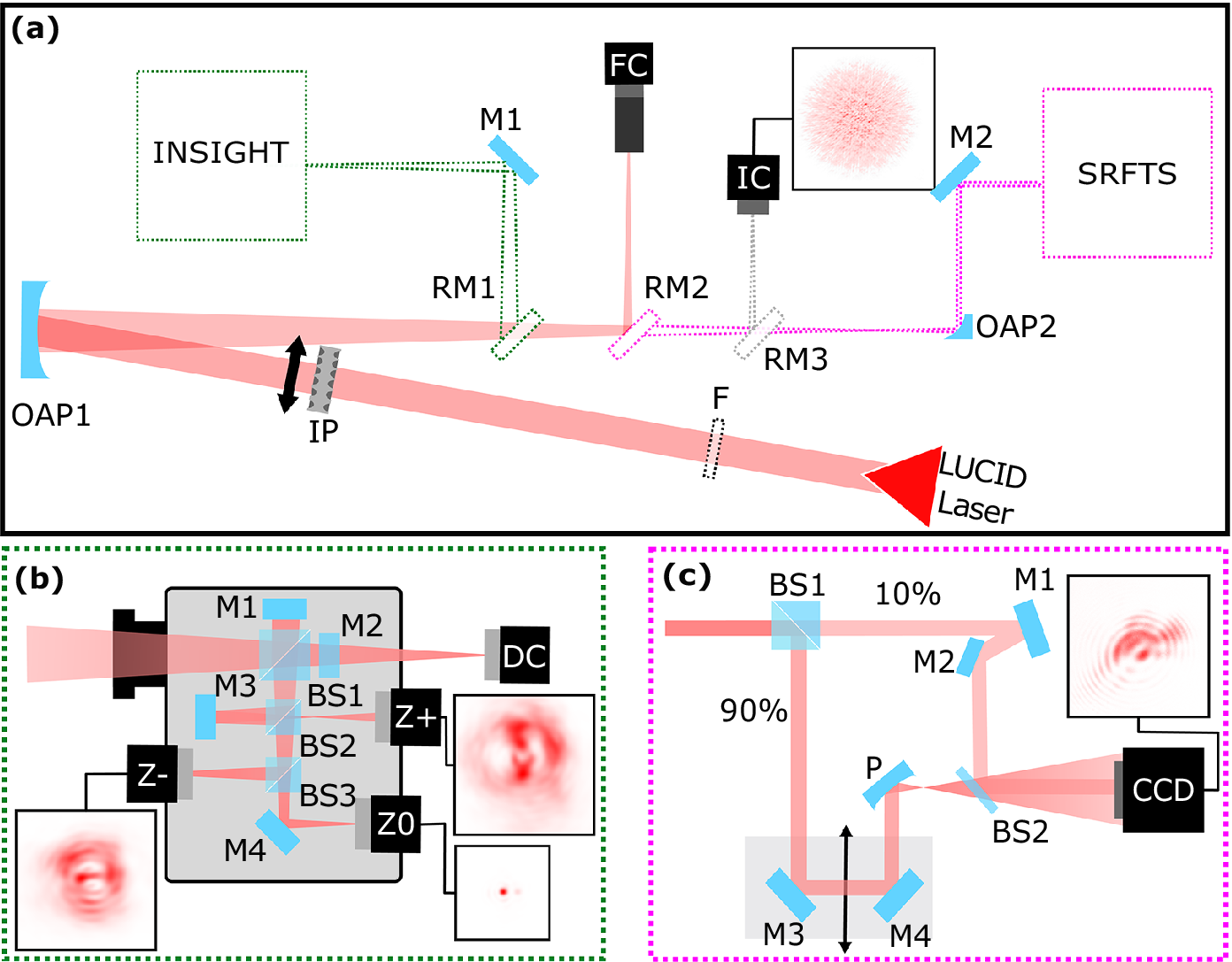
For this experiment, the beam was directed to an optical table in air, as shown in Figure 2. The figure shows an overview of the experimental setup, with the beam path shown starting from the red triangle. Prior to focusing, there is space for the spectral filter (F). After that, close to the focusing optic, is the insertion point of the IMPALA mask (IP). The beam is then focused by a 4-inch off-axis parabolic mirror (OAP1) with an off-axis angle of 12.8° and an apparent focal length of 1029 mm. Focusing of the pulses inside the INSIGHT device was achieved directly using the off-axis parabolic mirror, assisted by two flat 2-inch mirrors (RM1 and M1 in Figure 2(a)). Alternatively, the focal plane can be imaged using a focus camera with a 10× microscope objective (FC1), by redirecting the converging beam with another 2-inch folding mirror (RM2). The retractable mirror RM3 was used to direct the focused beam to the camera (IC) of the IMPALA device. Finally, the beam can be directed to a second off-axis parabolic mirror (OAP2) with a diameter of 1/2 inches, an off-axis angle of 90° and an apparent focal length of 50.8 mm that is used to re-collimate the beam for diagnosing it using the SRFTS device (magenta inset). The working principles of the aforementioned methods for STC characterization, namely IMPALA, INSIGHT and SRFTS, are detailed in the sections below. All measurements were performed with the unfiltered spectrum and with the insertion of a 2-inch long-pass filter with a cutoff wavelength of 850 nm (Thorlabs FGL850S) to increase the spectral dynamic range of the STC reconstruction.
(a) Schematic of the experimental setup. The laser path is shown, as well as the spectral filter (F), IMPALA mask (IP), and focusing off-axis parabola (OAP1). A removable mirror (RM1) channels the laser into the INSIGHT measurement. A removable mirror (RM2) sends the beam to a focused beam camera monitor (FC). A different removable mirror (RM3) channels the beam to the focal spot/IMPALA camera (IC). Finally, without both mirrors the beam goes to another off-axis parabola (OAP2) and is steered into the SRFTS measurement. (b) Detailed schematic of the INSIGHT measurement: mirrors M1 and M2 together with BS1 form a Michelson interferometer. Mirror M3 and BS2 are used to look after the focal spot on the Z+ camera. BS3 and M4 redirect the beam towards Z– and Z0 cameras. The direct camera (DC) is used for pointing stabilization. (c) Detailed schematic of the SRFTS measurement: BS1 is a 10/90 beam splitter cube, M denotes flat mirrors, the arrow denotes movement of the piezo stage, P is a 50 mm focusing parabola, BS2 is a 2% reflection beam splitter and CCD denotes the camera. The inserts exemplify recorded raw images of the cameras.

Figure 2. Long description
A three-panel diagram showing optical layouts.
Panel a: The main schematic. A L U C I D Laser source at the bottom right sends a red beam through a spectral filter F and an I P mask to an off-axis parabola O A P 1. The reflected beam passes through three removable mirrors. R M 1 redirects the beam to mirror M 1 and into the I N S I G H T measurement block. R M 2 redirects the beam to a focused beam camera F C. R M 3 redirects the beam to the focal spot camera I C, which shows an inset of a red diffuse spot. If all mirrors are removed, the beam hits O A P 2 and enters the S R F T S measurement block.
Panel b: Detailed I N S I G H T schematic. The beam enters a gray housing. B S 1 splits the beam between mirrors M 1 and M 2 to form an interferometer. B S 2 and mirror M 3 direct light to the Z plus camera. B S 3 and mirror M 4 direct light to the Z minus and Z 0 cameras. A direct camera D C is positioned at the exit. Insets show red interference patterns for Z minus, Z plus, and Z 0.
Panel c: Detailed S R F T S schematic. The beam enters B S 1, splitting into 10 percent and 90 percent paths. The 90 percent path reflects off mirrors M 3 and M 4 on a moving piezo stage, then hits a focusing parabola P. The 10 percent path reflects off mirrors M 1 and M 2. Both paths converge at B S 2 before entering a C C D camera. An inset shows a red diffraction pattern recorded by the C C D.
2.2 INSIGHT measurement setup
The INSIGHT measurement technique[ Reference Borot and Quere 31 ] relies on spatially resolved spectral retrieval of laser pulses via Fourier transform spectroscopy, using only beam profiles recorded in the focal plane (Z0) and in two additional planes located a few Rayleigh ranges away from focus (Z+ and Z–). The approach consists of finely scanning the temporal delay between each pulse and an identical reference replica. Once the spectrally resolved beam profiles are obtained both at focus and out of focus, a GS-type algorithm[ Reference Gerchberg 32 ] can be applied to reconstruct the spectrally resolved wavefront.
The method was implemented using the commercial INSIGHT Quadro system (SourceLab). The instrument incorporates, besides the three cameras for Z0, Z– and Z+ beam profiles, a dedicated pointing-tracking camera (PTC in Figure 2) that monitors the pulse direction during the scanning process, enabling compensation for pointing fluctuations of the laser. To ensure a broad spectral acceptance, the optical components of the Michelson interferometer were upgraded with broadband optical components (i.e., silver mirrors, including the leakage mirror for the pointing-tracking camera and broadband filters).
Focusing of the pulses inside the INSIGHT device was achieved directly using the off-axis parabolic mirror, assisted by two flat 2-inch mirrors (RM3 and M4 in Figure 2). Neutral-density filters were positioned at the device entrance to control the incident pulse energy.
The reconstruction of the three-dimensional (3D) temporal shape of the pulses starts from the spectral slices of the far-field measured with the INSIGHT device for the two measurements: one without any spectral filter and one with an 850 nm filter. The spatially integrated spectrum of a given INSIGHT measurement is reconstructed, and the constant residual noise from the data is estimated. Then the constant noise, up to 25% in our measurements, is removed from each far-field slice. The noise is a flat floor, removed per individual spectral slice. Each slice is then normalized to its integrated signal, so that the total intensity of each slice is equal to one. The normalized datasets are then stitched together, providing increased spectral coverage. After stitching, each spectral slice is rescaled according to the corresponding spectral intensity measured independently with a calibrated spectrometer. The result is an accurate 3D reconstruction of the pulse’s spatio-spectral profile, with improved dynamic range, and respecting the spectrum as measured with the spectrometer. Finally, a Fourier transform is applied along the spectral axis at every point in the XY plane, resulting in the spatio-temporal reconstruction of the pulse. This step can be performed assuming a flat spectral phase, or with the measured spectral phase from the d-scan device.
2.3 IMPALA measurement setup
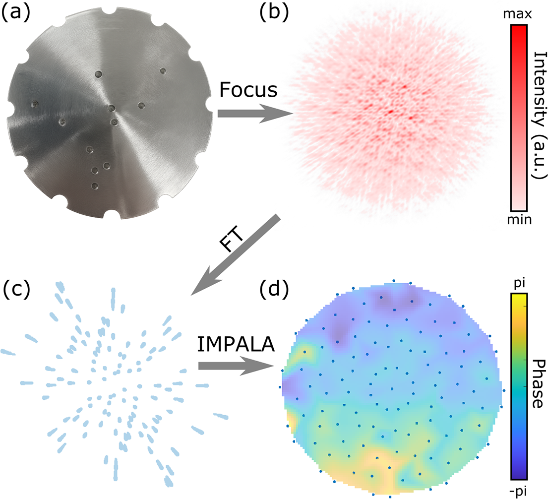
The principle of the IMPALA technique is to algorithmically, rather than optically, separate out spectral information in the Fourier plane, thus allowing for a minimal experimental setup. The beam is passed through a specially designed pinhole mask, shown in Figure 3(a), and focused by the focusing optic used in the experimental setup. The resulting interference speckle pattern, shown in Figure 3(b), is captured by an imaging system – in this case the existing focal spot imaging of the experiment. A spatial Fourier transform is then performed on the speckle pattern. In the Fourier plane, this results in a central peak, corresponding to the intensity envelope, and streaks symmetrically distributed around the central peak, as is shown in Figure 3(c). The key to the IMPALA technique is that inside of these streaks, information about the behavior of different wavelengths is spatially separated, with the ‘redder’ components of the beam closer to the central peak when compared to the ‘bluer’ components. The IMPALA algorithm then isolates different spectral bands and performs the GS iterative phase retrieval algorithm to reconstruct a quasi-monochromatic wavefront, shown in Figure 3(d), for each spectral band inside of the beam. These wavefronts can then be stitched together, giving the spectrally resolved wavefront of the laser. Additional details of the IMPALA algorithm can be found in Ref. [Reference Smartsev, Liberman, Andriyash, Cavagna, Flacco, Giaccaglia, Kaur, Monzac, Tata, Vernier, Malka, Lopez-Martens and Faure41].
Overview of the IMPALA technique. (a) Pinhole mask designed by a genetic algorithm for the LLC laser system measurement. (b) Raw interference speckle pattern for 760 nm obtained by passing the beam through the mask and focusing. Red colorscale shows relative intensity. (c) Streak pattern obtained by performing a spatial Fourier transform on the interference speckles. These streaks contain spatially separated chromatic information about the beam. (d) Retrieved wavefront for one particular spectral band of the LLC laser. Colorscale shows phase from -π to π. Blue dots indicate the spatial points at which the wavefront is sampled.

Figure 3. Long description
The diagram is organized into four panels labeled a through d.
Panel a, top-left, shows a circular metallic pinhole mask with a brushed texture. It features several small circular apertures arranged in a non-uniform pattern and semi-circular notches around its perimeter. An arrow labeled Focus points right to panel b.
Panel b, top-right, displays a raw interference speckle pattern. It appears as a dense, circular cloud of red dots on a white background. A vertical color scale to the right indicates Intensity in a.u., ranging from min in white to max in dark red. An arrow labeled F T points diagonally down to panel c.
Panel c, bottom-left, shows a streak pattern consisting of numerous light blue elongated dots radiating outward from a central point. An arrow labeled I M P A L A points right to panel d.
Panel d, bottom-right, presents the retrieved wavefront as a circular heat map. The colors transition from dark blue to yellow, representing phase values. A vertical color scale to the right is labeled Phase, ranging from minus pi at the bottom in dark blue to pi at the top in yellow. The circular map is overlaid with a grid of small blue dots indicating spatial sampling points.
A specialized mask was designed using the genetic algorithm described in Ref. [Reference Smartsev, Liberman, Andriyash, Cavagna, Flacco, Giaccaglia, Kaur, Monzac, Tata, Vernier, Malka, Lopez-Martens and Faure41]. This genetic algorithm yields, for a given laser and imaging system and for a given number of holes in the mask, the optimal hole arrangement that yields the minimal overlap of streaks in the Fourier plane. The mask can also be designed to evenly sample the beam with a given number of rotations. In the case of the LLC experiment, a mask with 10 holes in addition to the central hole was used and was designed to sample the beam over 12 rotations. The blue dots in Figure 3(d) show the locations along the beam that the wavefront was sampled at.
Inside of the experimental setup, the IMPALA mask (shown as IP in Figure 2(a)) was set up such that the beam passed through the mask immediately prior to hitting the OPA (OPA1 in Figure 2(a)). After focusing, the beam was guided by mirrors (RM2 in Figure 2(a)) onto the imaging system (FC in Figure 2(a)), which captured the resulting interference pattern. The mask was designed to be removable, such that it would not interfere with the other measurement techniques.
The data were taken with a FLIR BFLY-PGE-31S4M camera that has 2048×1536 pixels, a pixel size of 3.45 μm and a Sony IMX265 sensor. Data were taken with 12 rotations of the IMPALA mask to ensure good spatial coverage of the beam. The data were taken with no filter and with the 850 nm filter. The beam was attenuated to the minimal point at which the interference signal does not saturate the camera during the measurement. There was an attenuation difference of two orders of magnitude obtained using neutral density (ND) filters between the no filter case and the 850 nm filter case, with the 850 nm filter having the lower attenuation.
2.4 SRFTS measurement setup
Both the INSIGHT and IMPALA measurements were carried out in the focus. In the setup a parabolic mirror was used to focus the beam. To perform the same measurement using the SRFTS device the beam needed to be re-collimated. For this purpose, a parabolic mirror (OAP2 in Figure 2) was placed behind the focus to obtain a beam of appropriate size. Additional attenuation was performed by routing the beam using a wedge at the entrance of the device.
The SRFTS setup is based on that presented in Ref. [Reference Miranda, Kotur, Rudawski, Guo, Harth, L’Huillier and Arnold29] and is schematically displayed in Figure 2(c). The collimated beam is split into two, the unknown and the reference beams, by an uncoated 10/90 beam splitter cube (BS1). The unknown beam propagates undisturbed through the interferometer. The reference beam is first sent to a delay stage, piezzosystemjena PX499SG, where the length of the reference arm is controlled. Then the reference beam is focused by an OPA (P) with a focal length of 50 mm. With a short focal length and long propagation (500 mm) afterwards, the beam is greatly expanded at the position of the detector, providing a clean and homogeneous spherical reference wavefront. The unknown beam and the generated reference beam are recombined, using a 2% reflection beam splitter (BS2). The use of the unbalanced beam splitter helps to balance the optic intensity of the two beams at the camera, as the reference beam is greatly expanded. This optimizes the fringe contrast and thus the overall signal-to-noise ratio (SNR). A charge-coupled device (CCD) camera, FLIR GRASSHOPPER 3 89S6M-C, is used to record the spatial interference for each delay step. Simultaneously, the dataset contains the time interferogram for each pixel, allowing reconstruction of the spectrum. The interference between the reference beam and the known beam forms a Newton’s ring-like interference pattern. By varying the time delay, the interference pattern oscillates and forms an interferogram over the whole spatial position. Therefore, the spatial spectra and phase can be retrieved by Fourier transform analysis. Assuming a homogeneous reference beam with a spherical phase origin at the focus of the parabola, the phase of the unknown beam and its individual colors can be obtained.
As with the INSIGHT and IMPALA measurements, the SRFTS measurements were carried out without a filter and with a chromatic long-pass filter, cutting the spectrum below 850 nm. The attenuation on the camera was adjusted to optimize contrast while avoiding saturation.
3 Results and discussion
3.1 Enhanced spectral bandwidth of the INSIGHT device
The large variation in spectral intensity across the spectral range corresponds to a significant variation in the SNR of the INSIGHT measurements at different spectral ends, impacting the accurate reconstruction of the temporal shape for the pulse. To address this issue, we introduced the 850 nm spectral cutoff filter to suppress the intense, blue part of the pulse spectrum and to access the spectral components with lower intensity. In the presence of the 850 nm filter, the energy of the spectrally clipped pulses entering the INSIGHT device was increased by removing a neutral-density filter from the beam path.
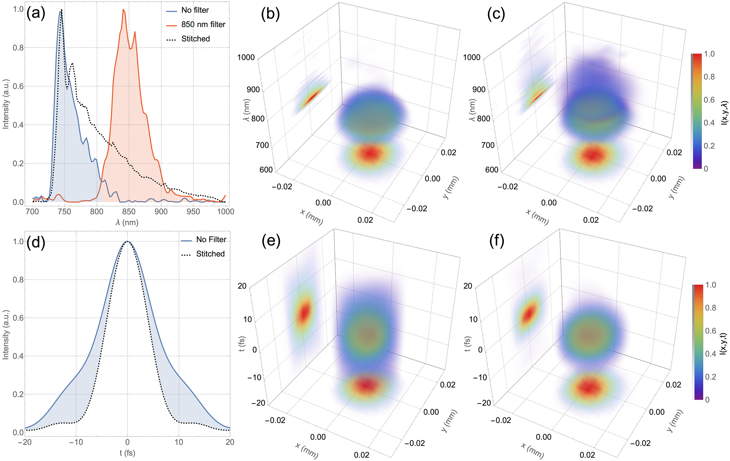
In Figure 4(a), the two spatially integrated spectra recovered by the INSIGHT device are depicted for the cases of no filter and 850 nm cutoff filter, after constant noise removal (see Section 2.2 for the step-by-step data processing description). The spectrum obtained from an independent spectrometer measurement is also shown as a dashed line. For a comprehensive spectral description of the two measurements, Figure 4(b) depicts the spectrally resolved far-field of the INSIGHT measurement without a spectral filter. It corresponds to the blue curve in Figure 4(a). Figure 4(c) depicts the spectrally resolved far-field corresponding to the stitched reconstruction using the spectral intensity represented with dashed line in Figure 4(a). Both the raw data and the rendering code are available upon request.
Spectral (a)–(c) and temporal (d)–(f) properties inferred from the measurements. (a) Spatially integrated INSIGHT spectra from the measurements without a filter and with an 850 nm cutoff filter (solid lines with shading), and the spectrum measured with a spectrometer (dotted line). Spatio-spectral reconstruction of the direct INSIGHT measurement (raw data) (b) and stitched data from the two measurements (raw data) (c). (d) Fourier-transform-limited (FTL) pulse duration obtained from the spatially integrated direct INSIGHT measurement (solid line with shading) and from the spectrometer data (dotted line). Spatio-temporal reconstruction using the direct INSIGHT measurement (e) and using the stitched data from the measurements (f).

Figure 4. Long description
A six-panel figure labeled a through f.
Panel a is a 2D line graph of Intensity in a.u. versus wavelength lambda in nanometers. It shows three curves: a blue shaded peak centered at 750 nanometers (No filter), an orange shaded peak centered at 850 nanometers (850 nm filter), and a black dotted line (Stitched) encompassing both regions.
Panel d is a 2D line graph of Intensity versus time t in femtoseconds. A solid blue line with shading shows a broad pulse centered at 0 femtoseconds, while a black dotted line shows a narrower Fourier-transform-limited pulse.
Panels b and c are 3D spatio-spectral plots with axes x in millimeters, y in millimeters, and lambda in nanometers. They show a central translucent blue-green volume representing intensity I(x, y, lambda). Panel b shows a single spectral component, while panel c shows the stitched data with a larger vertical extent. Projections are visible on the x-y plane (red-yellow circular heat map) and the lambda-x plane.
Panels e and f are 3D spatio-temporal plots with axes x in millimeters, y in millimeters, and time t in femtoseconds. They show a central volumetric pulse. Panel e represents the direct measurement, and panel f represents the stitched data. Both include heat map projections on the x-y and t-x planes, with intensity color-coded from purple (0) to red (1.0) on a vertical color bar to the right of the panels.
To understand the effects on the temporal reconstruction of the pulses, we assumed a spectrally flat phase and computed the pulse duration for the case of the INSIGHT measurement without a spectral filter and for the case of the stitched data, as depicted in Figure 4(d). A significant reduction in the Fourier-limited pulse duration is observed in the case of the spectrum obtained from the direct INSIGHT measurement (blue line) compared to the spectrum recorded with the spectrometer (dotted line): from 12.4 to 9.3 fs FWHM, corresponding to an absolute duration correction of 3.1 fs, a reduction by a factor of 1.33.
Figures 4(e) and 4(f) depict the spatially resolved temporal intensity distribution in the focus reconstructed from the direct INSIGHT measurement (Figure 4(c)) and from the two measurements stitched. A significant reduction in the focal volume is observed in the case of the stitched measurement, as expected for a broader bandwidth and a more realistic reconstruction.
The results show that the INSIGHT device, even when adapted with silver mirrors and broadband optics, failed to accurately reconstruct the LUCID laser, due to the limitation of the sensor.
The significant discrepancy between the spectrometer-given pulse duration and the pulse duration obtained from the no filter measurement also impacts the value of the peak intensity. Integrating the curves in Figure 4(d), and assuming the same energy for the pulse in the two cases, the peak intensity retrieved from the stitched INSIGHT measurement is 55% larger than the one from the direct INSIGHT measurement. This value is similar (57%) also when considering the full 3D integration of the reconstructed pulses in Figures 4(e) and 4(f).
3.2 Enhancing spectral bandwidth of the IMPALA device
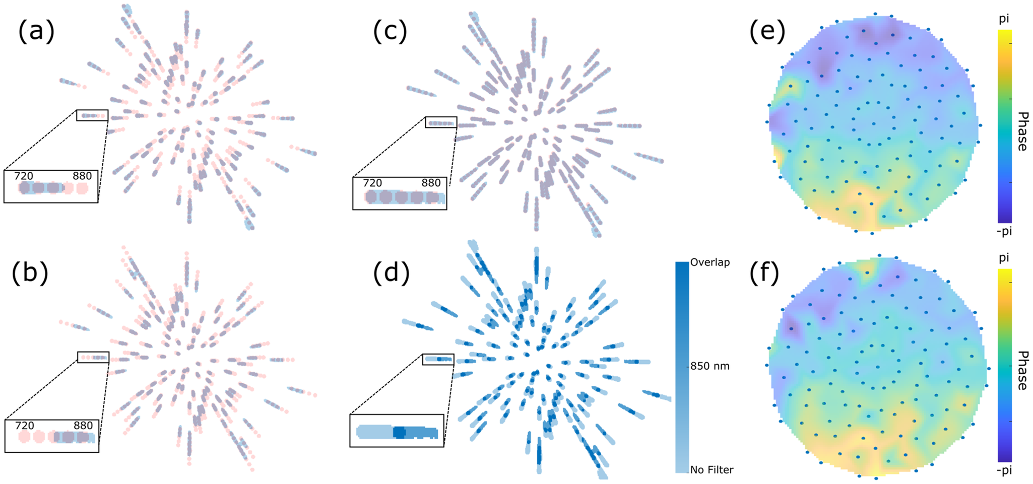
For the IMPALA measurement, the raw interference speckle patterns were Fourier transformed to obtain the streaks in the Fourier plane, as described above. Figure 5(a) shows the experimentally obtained streaks for the LLC beam with no spectral filters present and for one particular orientation of the IMPALA mask. The streaks shown in blue have been normalized to have a value of unity where signal is present and a value of zero where no signal is present. In addition, the figure shows the simulated quasi-monochromatic streaks centered at different wavelengths, ranging from 720 nm (the most distant from the center) to 880 nm (closest to center) in 40 nm steps. Each of the simulated streaks is shown as a pink circle, with the shorter wavelength further from the center and longer wavelength closer to it. The simulated streaks provide a reference about what sections of the spectrum the IMPALA device is retrieving. The insert shows an enlarged example of one streak, for emphasis. As can be seen in the insert, the recovered spectrum of the streaks spans about 720–820 nm. From the measured spectrum of the LLC laser system in Figure 1(c), it is clear that, as with the INSIGHT technique, a significant portion of the spectrum is lost due to insufficient signal being present at the ‘redder’ wavelengths of the laser.
Impact of dynamic range enhancement on IMPALA data. (a) IMPALA streaks (blue) for the LLC laser without any spectral filtering as well as the simulated quasi-monochromatic streaks centered at 720, 760, 800, 840 and 880 nm (shown in pink). The insert shows an enlarged example of a streak. (b) IMPALA streaks for the LLC laser with the 850 nm spectral filter in place. (c) IMPALA streaks obtained by summing the results of the no filter and 850 nm filter cases. All areas with signal are normalized to the same value. (d) IMPALA streaks obtained by summing the results of the no filter and 850 nm filter cases. The blue colorbar shows the places where just one signal is present or where overlapping signals are present. (e) Retrieved 760 nm wavefront for the LLC laser. Colorscale shows phase from -π to π. Blue dots indicate the spatial points at which the wavefront is sampled. (f) Retrieved 840 nm wavefront.

Figure 5. Long description
The figure consists of six panels labeled a through f.
Panel a shows a radial distribution of I M P A L A streaks. Blue streaks represent the unfiltered L L C laser, while pink streaks represent simulated quasi-monochromatic streaks from 720 to 880 nanometers. An inset box zooms in on a single streak, showing a horizontal gradient from 720 on the left to 880 on the right.
Panel b displays streaks for the L L C laser with an 850 nanometer spectral filter. The streaks are concentrated towards the outer edges of the radial pattern compared to panel a. The inset shows the signal shifted toward the 880 nanometer end of the scale.
Panel c shows the summation of the no-filter and 850 nanometer filter cases, resulting in a denser radial pattern of light purple streaks. The inset shows a continuous horizontal bar spanning the 720 to 880 nanometer range.
Panel d presents the same summed data as panel c but uses a blue colorbar to indicate signal presence. The colorbar on the right ranges from light blue for No Filter to dark blue for Overlap. The inset shows the overlapping regions in the darkest blue.
Panel e is a circular heatmap of the retrieved 760 nanometer wavefront. The phase ranges from negative pi in dark purple to pi in bright yellow. Blue dots are arranged in concentric rings from the center to the perimeter to indicate spatial sampling points. The phase is predominantly green and yellow in the lower half and purple in the upper left.
Panel f is a circular heatmap of the retrieved 840 nanometer wavefront, following the same color scale and sampling dot pattern as panel e. The phase distribution is similar to panel e but shows slight variations in the intensity of the yellow and purple regions.
When the 850 nm filter is introduced into the laser path, the IMPALA streaks are significantly altered. As can be seen in Figure 5(b), the spectral range of the streaks is now about 800–900 nm, representing a significant redshift over the previous signal. This is due to the fact that with the 850 nm filter in place, attenuation of two orders of magnitude obtained by neutral density filters was removed, thus allowing the ‘redder’ part of the beam to have a strong enough signal to be detected. The signal above 900 nm was still too weak to detect. The camera has a two times lower spectral response at 900 nm in comparison with that at 800 nm. This reduced spectral sensitivity, together with the spectral shape of the pulses, having lower spectral intensity above 850 nm, and decreasing, corresponds to a drastic reduction of the SNR at the 900 nm wavelength and longer. Note that the spectral filter has a good spectral response, with more than 70% transmission and up to 90% in the region with wavelengths above 850 nm, partially compensating for the reduced spectral sensitivity of the camera.
Figure 5(c) shows the result of summing the experimental no filter streaks and 850 nm filter streaks and then normalizing the result in the same way as in Figures 5(a) and 5(b). As can be clearly seen, with the addition of the two results the signal now spans from 720 to 900 nm, covering a far larger span than each individual measurement contained. This is further fleshed out in Figure 5(d), which again shows the summed data of the no filter streaks and the 850 nm filter streaks. Here, however, rather than normalizing to unity, the colorbar in the figure shows the areas in which only the no filter data are present, only the 850 nm filter data are present and where both datasets overlap.
It is important to note that the no filter data and the 850 nm filter data were processed in exactly the same way and no reorienting was introduced in order to align the two different streak patterns. Simply by numerically adding the results together, the streaks naturally align in a near-perfect manner. Furthermore, the retrieved wavefronts for 810 nm with and without the filter were compared and were found to be closely aligned with each other, further reinforcing this point. This clean alignment indicates that introducing the spectral filter effectively expands the range of the measurement while introducing minimal distortion to the data itself.
Figure 5(e) shows the retrieved monochromatic wavefront at 760 nm, obtained using the IMPALA device. The colorscale shows phase from -π to π and the blue dots indicate the spatial points at which the wavefront is sampled. Figure 5(f) shows the retrieved monochromatic wavefront but at 840 nm. The ability to retrieve wavefronts from a broad range of frequencies, beyond the range of that afforded by the measurement with no filters, shows the advantage of the spectral enhancement method.
3.3 Enhancing the spectral bandwidth of SRFTS
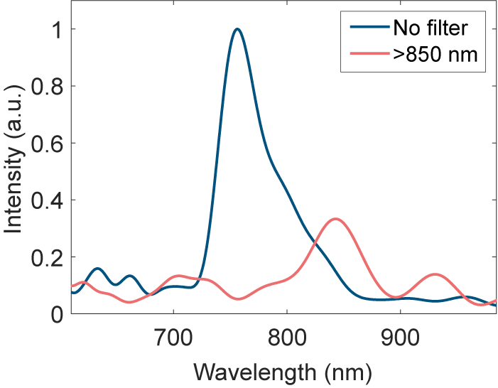
SRFTS measurements were taken without and with the spectral filter. However, due to the long beamline, the beam pointing had a strong influence on the SRFTS measurement results. Unlike the IMPALA and INSIGHT measurements, the SRFTS setup has different magnifications for the unknown beam and the reference beam; therefore, the beam pointing is also magnified differently. This cannot be processed with post-alignment like in the INSIGHT technique. This issue invalidates the assumption that the reference beam is identical in each frame. Therefore, the full STC retrieval result is not reliable in these measurements. However, we still can retrieve spatially averaged spectra out of the measurement results, as shown in Figure 6, with and without an long-pass filter. To compensate the loss of photons, we remove the ND3 (3 dB) filter to maximize the dynamic range of the camera analog-to-digital converter when using the long-pass filter. This approach helps to increase the fringe contrast and therefore the SNR for the 800 to 880 nm spectral component. This boost of the effective SNR can be observed by normalizing the noise floor to a similar level, as shown in Figure 6. Instead of normalizing each spectrum to unity, only the unfiltered spectrum has been normalized, while the other has been normalized and then matched to that noise level.
Retrieved spectrum from the SRFTS measurement with no filter (blue) and with the long-pass filter at 850 nm (red).

Figure 6. Long description
A line graph plots Intensity in a.u. on the vertical Y axis from 0 to 1 against Wavelength in n m on the horizontal X axis from approximately 600 to 1000.
* The blue line labeled No filter shows a dominant, sharp peak reaching an intensity of 1.0 at approximately 750 n m. It has smaller secondary peaks around 650 n m and 700 n m, and the signal drops to near zero beyond 850 n m.
* The red line labeled greater than 850 n m shows the effect of the long-pass filter. The major peak at 750 n m is suppressed to near zero. Instead, the signal rises to a primary peak of approximately 0.35 intensity at 850 n m, followed by a smaller peak of 0.15 intensity at 930 n m.
A legend in the top right corner identifies the blue line as No filter and the red line as greater than 850 n m.
When comparing the two measurements, it is clear that the case without a filter (blue) yields a peak at 754 nm, which is shifted to 846 nm with the filter (red). Introducing a filter that mostly attenuates the blue part of the spectrum allows retrieval of red wavelengths that were not retrievable without the filters. The retrieved spectrum of the laser spans approximately from 720 to 850 nm, with a clear triangular shape. Introducing the chromatic filter shifts this to 800–880 nm.
Similar to the INSIGHT technique, each measurement and reconstruction is performed independently and the stitching is performed as the very last, final step. The computational time for the stitching itself is negligible compared to data taking (20 min for a typical scan) and reconstructing (1 h).
4 Conclusion
The centrality of the CMOS sensor to many spatio-temporal and spatio-spectral measurement methods is a significant barrier in the accurate reconstruction of few-cycle pulses in the near-infrared regime. As was shown, all three methods tested, INSIGHT, IMPALA and SRFTS, failed to accurately reconstruct the full spectrum of the pulse and therefore missed the spatio-spectral behavior of those wavelengths. The solution shown for all three methods, the introduction of chromatic filters, succeeded in overcoming this limitation by allowing the wavelengths at which the CMOS is less sensitive to be amplified more and, therefore, to cross the signal-to-noise threshold of the detector. This solution can be further expanded by introducing more spectral filters, allowing the stitching of even larger bandwidths.
In the future, another possible solution would be to manufacture spectral filters that pre-compensate for the specific CMOS response so that, by placing them before the sensors, the CMOS’s spectral response would be flattened. This, however, would be a solution tailored to a specific system while the solution used in this work is easily implementable in any laser system.
By enabling the extension of existing metrology methods to few-cycle pulses, this work lays the ground for the accurate reconstruction of those pulses. This ability is both critical to the avoidance of unwanted spatio-temporal/spatio-spectral effects that could limit the quality of the pulse and also to the accurate implementation of such effects for advanced spatio-temporal shaping of the laser pulse.
Author contributions
The joint experiment was conceptualized and planned by D.U., A.L., O.L., C.Ar. and V.M. The manuscript was prepared under the supervision of A.L. with input from all the authors. All authors except V.M. participated in the experiment. All authors participated in preparatory work for the experiment. The LASERLAB grant was obtained by D.U. Funding for the ELI-NP team was obtained by D.U. who also supervised the team; funding for the LLC team was obtained by O.L. and C.Ar. who also supervised the team; funding for the Weizmann team was obtained by V.M. and the team was supervised by A.L. and V.M.
Acknowledgements
The joint experiment received funding from LASERLAB-EUROPE (Grant Agreement No. 871124, European Union’s Horizon 2020 Research and Innovation Programme). The ELI-NP team was funded by the Romanian Ministry for Research, Innovation and Digitalization through the ELI-NP IOSIN program, through project ELI-RO/DFG/2025_013 IATP-NP 2.0 and ELI-RO/AMIPulse funded by Institute of Atomic Physics Romania, and through the Nucleu program PN 23 21 01 05. The Weizmann team was funded by the Schwartz/Reisman Center for Intense Laser Physics, the Benoziyo Endowment Fund for the Advancement of Science, the Israel Science Foundation, Minerva, the Wolfson Foundation, the Schilling Foundation, R. Lapon, Dita and Yehuda Bronicki and the Helmholtz Association. The LLC team was supported by the Swedish Research Council (VR 2019-04784, 2024-05698), the Knut and Alice Wallenberg Foundation (KAW 2019.0318, 2020.0111) and the European Union’s Horizon Europe Research and Innovation Programme (Grant Agreement No. 101073480). The authors thank Dr. Slava Smartsev for constructive conversations about the IMPALA measurement. The authors thank Prof. Claes-Göran Wahlström for assistance in the planning and execution of the experiment.

 Open access

