1. Introduction
In pay-as-you-go (PAYG) pension systems, the financial balance depends on the proportions of active and inactive people in the population.Footnote 1 According to the projections of the United Nations (United Nations – UN, 2022), the median dependency ratio of people over 65 years old per 100 people between 20 and 64 years of age will double in the next 30 years and more than triple at the end of the century in middle-income countries. This process of demographic transformation places increasing pressures on the sustainability of PAYG systems in these countries, making the introduction of extensive reforms inevitable.Footnote 2
In general, structural reforms of these systems impact a wide range of economic dimensions. In addition to affecting labor supply, aggregate savings, and economic growth, reforms in PAYG systems change the income distribution across generations, impacting differently permanent income and rates of return of social security assets for agents born in different cohorts. In developing countries, in particular, where heterogeneity among workers is high (e.g. economies with high educational inequality and a high fraction of prime age individuals with informal ties to the labor market), reforms in PAYG systems can also greatly impact the permanent income and rates of return of different groups of agents in the same cohort.Footnote 3 Quantifying changes in permanent income inequality and equity in rates of return is thus an important exercise when there is concern as to the effects of different PAYG systems on vertical (between groups of agents) and horizontal (between generations) inequality.
The most adopted type of PAYG system is that of a Defined Benefit (DB) structure. Typically, the DB system offers high benefits relative to the taxation levels and operating rules of this system, which generates growing deficits over time, especially in a context of accelerated demographic transformation.Footnote 4 Furthermore, with the aim of compensating agents with lower contributory densities (e.g., women and informal workers), DB replacement rates commonly include a component that is independent of the number of contributions. Despite playing a redistributive role, this component tends to increase fiscal imbalances and generates heterogeneity in rates of return between groups of agents in the same cohort and, due to economic trends and shocks, also between different cohorts.
To deal with the financial unsustainability of the DB system, some countries (e.g., Sweden, Italy, Poland, Norway, and Latvia) reformed their PAYG systems by adopting a Defined Contribution (DC) structure. In this system, agents contribute to an individual non-financial (or notional) account that is remunerated with some economic indicator (e.g., the average wage growth rate, as in Sweden). When retired, the individual receives a lifetime annuity whose value depends on the total amount accumulated in his/her notional individual fund at the time of retirement and the life expectancy of the agent’s birth cohort.Footnote 5 By construction, a DC system of this type does not affect permanent income inequality and inequity of returns between agents. In this sense, the DC system is neutral from both an intra- and inter-generational perspective.Footnote 6 However, the DC system tends to generate low-value benefits for agents who have low contributory densities or low wages (or both), which makes it an unsuitable system for developing countries.Footnote 7 In this article, we propose a new mixed system that combines features of DB and DC systems.Footnote 8 More specifically, we defined a formula for calculating retirement benefits that combines the component that does not depend on the number of contributions of the DB system with the individual fund component of the notional DC system. This combination of components makes it possible to mix the redistributive role of the DB system with the neutrality of the DC system.Footnote 9
Many countries in different regions of the world incorporate a non-contributory pillar in their social security systems that offers a minimum benefit to those who do not meet regular retirement requirements. Often linked to the minimum wage (e.g., Brazil, Colombia, and other Latin American countries; see Gill et al., Reference Gill, Packard and Yermo2005), this floor aims to guarantee a minimum income that avoids poverty in the elderly phase of life. Typically financed with general taxes, this pillar benefits the most vulnerable workers and in developing countries accounts for a high proportion of social spending. In addition, it tends to represent a disincentive to contributions to social security, which has repercussions on revenues of PAYG schemes.
The theoretical and empirical literature that assesses the economic effects of public pension systems is quite extensive.Footnote 10 More related to our study, Auerbach and Lee (Reference Auerbach and Lee2011) analyze how various stylized PAYG programs distribute the risks of demographic and economic shocks across generations. The analysis is conducted in a stochastic environment for financially-balanced systems, and considers the steady-state situation. Auerbach et al. (Reference Auerbach, Kueng, Lee and Yatsynovich2018) use a model of overlapping generations with balanced government budget to compare the performance of several stylized PAYG systems in the distribution of intergenerational risks arising from specific shocks in productivity, fertility, mortality, and migration. Ludwig and Reiter (Reference Ludwig and Reiter2010) also use a model of overlapping generations to investigate how different PAYG designs affect intergenerational well-being from specific fertility shocks. The analysis of these studies is carried out for the representative agent of each generation, which implies that there is no intragenerational heterogeneity, making their frameworks and results more appropriate for developed countries. Unlike these studies, our analysis evaluates the performance of different types and designs of stylized PAYG systems for developing countries, where agents are more heterogeneous, inserted in a labor market with informal employment (i.e., where agents do not always contribute to social security), and in which large portions of the population reach the elderly stage in poverty. To take these characteristics into account, our framework incorporates several relevant dimensions. First, recognizing the differences in labor market insertion between men and women, the analysis is carried out separately for the sexes. Second, we model both formal and informal labor income, as well as pension contribution patterns and the educational distribution of agents. Third, we incorporate the existence of a floor for retirement benefits and a pillar that guarantees a minimum income for the elderly poor. Finally, we consider different designs of the DB and the notional DC schemes, in addition to the aforementioned system that combines elements of these two structures. Naturally, the inclusion of all these dimensions makes our framework more complex but allows us to obtain a wealth of results for different types of agents, both within the same cohort and for different cohorts.
Methodologically, we use an empirical age-period-cohort model estimated with the Intrinsic Estimator proposed by Yang et al. (Reference Yang, Schulhofer-Wohl, Fu and Land2008). The estimates are used, together with some hypotheses about the age profile and trends by cohort, to project the future trajectories of labor income, the probability of contributing, and the educational distribution of observed and unborn cohorts for each type of agent. These trajectories make it possible to simulate the outcome variables of interest for different types and designs of PAYG systems, namely: measures of the financial imbalance over time, permanent income inequality, and rates of return of social security assets between types of agents and between cohorts. This analysis is carried out for two different contexts in relation to the financial stability of the systems. In the first one, we analyze PAYG structures in which system rules are pre-defined, and the financial imbalance is endogenous. In the second, contributions of active and inactive generations are endogenously adjusted over time so that the systems do not present imbalances. In this last context, we consider two adjustment rules: (i) the one proposed by Auerbach and Lee (Reference Auerbach and Lee2011) and Auerbach et al. (Reference Auerbach, Kueng, Lee and Yatsynovich2018) in which there is a proportional sharing mechanism between active and inactive groups to cancel the financial imbalance; and (ii) an adjustment inspired in the present German pension system, in which inactive groups share with the active ones the risks of imbalance and productivity gains after retirement.
We use data from Brazil, a country that, like other middle-income countries (especially in Latin America), is experiencing an accelerated population aging process, has significant skill heterogeneity in the workforce, and a large informal sector. The database is the Pesquisa Nacional por Amostra de Domicílios (PNAD – National Household Sample Survey) available between 1992 and 2015. PNAD is an annual cross-section sample representative of the country’s population and collects demographic and socioeconomic information, including labor income and formal-informal insertion in the labor market. Our simulations start in 2016 and cover the time horizon up to 2140. Unlike other studies (e.g., Auerbach and Lee, Reference Auerbach and Lee2011), we do not impose that the trajectory of the demographic profile was stationary and, therefore, we use the available projections – IBGE (2019) until the year 2030 and United Nations – UN (2022) from there until 2100 – making it possible to assess long-term effects of trends on the simulated systems.
In addition to this Introduction, the article contains three other sections. In the second, we present the age-period-cohort model, the way we project the trajectories of labor income, contributory density, and educational distribution of different types of agents across the cohorts, the basic rules of contributions and benefits (including those of the assistance pillar for the elderly poor), and the measures for our outcome variables of interest (for the context without financial balance). The third section is dedicated to the presentation of the results. Given the complexity of our framework and the different contexts regarding the imposition or not of financial balance, the presentation is carried out in subsections. In the first one, we allow for financial imbalances and exclude the benefit floor and the assistance pillar to analyze the performance of various PAYG schemes without the influence of discontinuities generated by these components. In the second subsection, we maintain the possibility of imbalances, but now include these components. In the third subsection, which maintains these components, we impose adjustments to balance the systems and introduce new measures to gauge their burden on active and inactive generations. The final section summarizes the results, points out some conclusions and indicates possibilities of using our framework for analysis of reforms in PAYG systems.
2. Methodology
In this section, we describe the basic methodological components that underlie our simulations. In subsection 2.1, we analytically describe the age-period-cohort (APC) structure that models the evolution of the three dimensions that constitute the backbone of the simulations, namely: wages, the probability of contributing to social security, and the probability of belonging to one of a set of educational groups. In subsection 2.2, we describe the data used for the estimation of the APC model and present the hypotheses on the patterns of the age, period, and cohort components that allow the construction of the future, out-of-sample trajectories of these three dimensions for each cohort and type of agent over their life cycle. These trajectories specify the (net) labor income stream and the contributory density of agents during their working life and therefore form the basis to compute retirement benefits or receipt of the assistance benefit. To compute these benefits, it is necessary to specify the set of rules of PAYG structures for payment of contributions and receipt of benefits. This is done in subsection 2.3, where we present the parameters and the basic variables of the systems, including retirement benefits for the Defined Benefit (DB) and the notional Defined Contribution (DC) structures. Finally, in subsection 2.4, we present the outcome variables that measure the performance of the systems in terms of the agents’ rate of return, inequality in permanent income, and aggregate deficit.
2.1. APC model for the agent profile
The profile of the agent of birth cohort  $c$, educational group
 $e$ and gender
 $g$, denoted by the triple
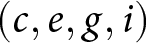
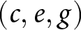 $\left( {c,e,g} \right)$, is characterized by the wage (
 $s$), the contributory pattern to social security (
 $p$), and the probability
 $z\left( e \right)$ of being in the group of education
 $e$. The age-period-cohort model (hereinafter, APC) allows decomposing the trajectory of (
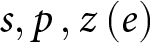 $s,p\,,z\left( e \right)$) according to variables indicating age, period (year), and cohort, which measure respectively the effects of age-indexed life cycle (
 $i$); the macroeconomic conditions of period (
 $t$); and long-term trends indexed to the cohort (
 $c = t - i$).
The heterogeneity of the agents’ profile is represented by the segmentation of the population into 6 education groups ( $e$) by gender (
 $g$), in a total of 12 groups, and by cohort (
 $c$).Footnote 11 Then, for agent
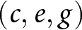 $\left( {c,e,g} \right)$ at age
 $i$, let
 ${p_{c,e,g,i}}$ be the probability of contributing to social security,
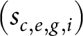
 ${s_{c,e,g,i}}$ the logarithm of the wage of those who contribute, and
 ${z_{c,g,e,i}}$ the probability of being in educational group
 $e$.Footnote 12 The APC model applied to the quantities that characterize the agent’s profile,
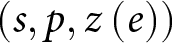 $\left( {s,p,z\left( e \right)} \right)$, can be written for the individual who belongs to cohort
 $c$, has schooling
 $e$, is of gender
 $g$ and is age
 $i$ in the following way. For
 $s$ and
 $p$, we write:
 \begin{equation}{s_{c,e,g,i}} = \,\alpha {1_{i,g}} + \beta {1_{t,g}} + \gamma {1_{c,g}} + \delta {1_{e,g}} + \,\varepsilon {1_{c,e,g,i}}\,\,\,\,\,\,g = 1,2\end{equation}
 \begin{equation}{p_{c,e,g,i}} = \,\alpha {2_{i,g}} + \beta {2_{t,g}} + \gamma {2_{c,g}} + \delta {2_{e,g}} + \,\varepsilon {2_{c,e,g,i}}\,\,\,\,\,\,g = 1,2\end{equation}
and for  $z\left( e \right)$, it is deemed a structural quantity that does not depend on the economic cycle and therefore it was estimated with a simplified version of the APC model that does not consider the period component:
 \begin{equation}{z_{c,e,g,i}} = \,\alpha {3_{i,e,g}} + \gamma {3_{c,e,g}} + \varepsilon {3_{c,e,g,i}}\,\,\,\,\,\,\,\,\,g = 1,2;e = 2, \ldots ,6\end{equation}
where  $\varepsilon k$,
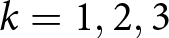 $k = 1,2,3$, represent the error terms. The equations for
 $s$ and
 $p$ are estimated separately by gender and those for
 $z$ by gender and education group. The parameter vectors
 $\alpha \left( i \right) = \left( {\,\alpha {1_{i,g}},\alpha {2_{i,g}},\alpha {3_{i,e,g}}} \right)$,
 $\beta \left( t \right) = \left( {\,\beta {1_{t,g}},\beta {2_{t,g}}} \right)$,
 $\gamma \left( c \right) = \left( {\,\gamma {1_{c,g}},\gamma {2_{c,g}},\gamma {3_{c,e,g}}} \right)$, and
 $\delta \left( e \right) = \left( {\,\delta {1_{e,g}},\delta {2_{e,g}}} \right)$ represent respectively the life cycle, the economic cycle, and the long-term trends associated with birth cohorts and schooling.
As is well known, the collinearity between the period, cohort, and age components makes the APC model unidentifiable. In the literature there are several approaches to circumvent this problem (see e.g., Schulhofer-Wohl, Reference Schulhofer-Wohl2018). We use the Intrinsic Estimator proposed by Yang et al. (Reference Yang, Schulhofer-Wohl, Fu and Land2008) which identifies the model using a general-purpose statistical method to estimate the age, period, and cohort coefficients.Footnote 13 As our exercises deal with long term outcomes of pension systems, so the cohort component must be extrapolated out of the sample. The period component captures transitory effects of the business cycle and will not be considered in the simulations. Based on external hypotheses, the cohort component will be projected for the cohorts that cannot be estimated in the sample, as discussed in section 2.2. It is worth mentioning that most of the cohorts considered in the simulations are projected, which reduces the importance of the estimated cohort coefficients.
2.2. Estimation and projection of the agent profile
The parameters that determine the agent’s profile presented in section 2.1 were estimated with data from the Pesquisa Nacional por Amostra de Domícilios (PNAD – National Household Survey Sample) between 1992 and 2015.Footnote 14 Conducted by the Instituto Brasileiro de Geografia e Estatística (IBGE – the Brazilian Census Bureau), the PNAD is a representative sample of the Brazilian population and provides information for the month of September of each year on a set of people’s characteristics (including gender, age, and education) as well as on their insertion in the labor market (including whether they have a formal job in the private sector or contribute to social security as self-employed), and income. As the PNAD is not a longitudinal survey, our analysis is based on a panel of agents defined by birth cohort ( $c$), schooling (
 $e$) and gender (
 $g$).
The APC model, presented in equations (1) to (3), determines the trajectory of each component of the agent’s profile, which is described by 14 variables: wage (2 sexes), contribution probability (2 sexes), and level-of-schooling group (5 educational categories and 2 sexes). For each variable, the model decomposes the profile trajectory into three temporal components (age, period, and cohort), respectively estimating the parameters:  $\alpha \left( i \right) = \left( {\,\alpha {1_{i,g}},\alpha {2_{i,g}},\alpha {3_{i,e,g}}} \right)$,
 $\beta \left( t \right) = \left( {\,\beta {1_{t,g}},\beta {2_{t,g}}} \right)$,
 $\gamma \left( c \right) = \left( {\,\gamma {1_{c,g}},\gamma {2_{c,g}},\gamma {3_{c,e,g}}} \right)$, and
 $\delta \left( e \right) = \left( {\,\delta {1_{e,g}},\delta {2_{e,g}}} \right)$, where the vectors
 $\left( {\alpha \left( i \right),\beta \left( t \right),\left( c \right)} \right)$ and
 $\delta \left( e \right)$ have 14 and 4 dimensions, respectively. The estimates of these parameters were obtained for the years
 $t = \left\{ {1992,1993,1995,\ldots,1999,\,2001,\, \ldots ,\,2009,\,2011, \ldots ,2015} \right\}$, a contribution horizon
 $i = \left\{ {20,\ldots,70} \right\}$, and cohorts
 $c = \left\{ {1942,\ldots,1982} \right\}$.Footnote 15
For the age profile of the agent, we assume that the age component  $\alpha \left( i \right)$ is the same for all future generations. The period component β(t) represents the effect of the economic cycle, it is assumed to be transitory, and is not considered in the projections. We adopt some hypotheses to project the contributory profile for ‘future’ cohorts, that is, those not included in the model estimation. The
 $\gamma \left( c \right)$ component is deemed to describe the effect of the long-term trend that captures the influence of preferences as well as technological and institutional factors. It was projected with a linear trend inspired by external sources and the APC model’s own results.Footnote 16 We assume that the profile of schooling in Brazil will reach in 2030 the OECD profile observed in 2008 (OECD, 2008), wage growth across cohorts will be equal to 1% – as estimated by Barbosa Filho and Pessoa (Reference Barbosa Filho and Pessoa2014) for the average growth rate in labor productivity between 1982 and 2012 – and formalization (i.e., the probability of social security contribution) will follow the same trend estimated in the model of 0.2% per year.Footnote 17 These values directly or indirectly define the trend growth of each component of the agents’ profile.
2.3. PAYG rules
The starting point in our analysis is a stylized pension system inspired in the PAYG scheme in force in Brazil after 2019.Footnote 18 We restrict the analysis to the system’s rules that apply to urban, private sector workers (including the self-employed), which represent 82% of the workforce in the country during our period of analysis.Footnote 19 We only consider pensions directly paid to the retired, so we disregard other related expenditures such as survivor pensions and other types of allowances.Footnote 20 The analysis incorporates an assistance component of social security systems – often called zero pillar (World Bank, 1994; Gill et al., Reference Gill, Packard and Yermo2005) – for low-income, old-age workers who do not meet the criteria for regular retirement.
In this stylized system, given the profile ( ${s_{c,e,g,i}},{p_{c,e,g,i}},{z_{c,e,g,i}}$) of the agent
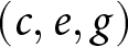 $\left( {c,e,g} \right)$ throughout his age
 $i$, the PAYG rules determine the contribution rate during the active period and age
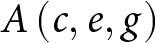 $A\left( {c,e,g} \right)$ from which the agent starts to receive an annuity
 ${b_{c,e,g}}$. In the sequel, we define the main variables and rules of the system. Table 1, at the end of this subsection, presents the values of the parameters on which these rules are based.
Parameters of the DB and DC systems of reference

Source: Constructed by the authors.
To describe the structure of the system, we divide the presentation of this subsection into three parts. In the first, we present a set of basic variables that will be used to construct various other variables that define the functioning of the system. The second part presents variables related to the contribution of agents to the pension system. The third part is devoted to presenting: (i) the rules that determine eligibility for regular retirement benefits and the assistance benefit, and (ii) how such benefits are calculated for both the DB and DC structures.
2.3.1. Basic variables
In this part, formed by equations (4) to (6), we describe basic variables such as the population and the value of the aggregate wage bill per year. The ratio of the latter to the former variable defines aggregate productivity in year t and is used to calculate the changes in productivity over time. We also define the evolution of the minimum wage, which is a variable that enters into various equations that determine pension contributions, eligibility rules and benefit calculations.
The population in period  $t$ can be expressed as the sum of population segments defined for agents at each age present in
 $t$:
 \begin{equation*}po{p_t} = \,\mathop \sum \limits_{c,g} \mathop \sum \limits_{i \in I\left( {c,t} \right)} po{p_{c,g,i}},\end{equation*}
where  $I\left( {c,t} \right) = \left\{ {i;\,c + i = t} \right\}$.
Based on the agents’ wages, the payroll is obtained by:
 \begin{equation}f{s_t} = \,\mathop \sum \limits_{c,e,g} \mathop \sum \limits_{i \in I\left( {c,t} \right)} {\text{exp}}({s_{c,e,g,i}})*{p_{c,e,g,i}}*{z_{c,e,g,i}}*po{p_{c,g,i}},\end{equation}
an aggregate variable that, together with that for population, define the productivity gain in period  $t$:
 \begin{equation}{y_t} = \frac{{\left( {f{s_t}/po{p_t}} \right)}}{{\left( {f{s_{t - 1}}/po{p_{t - 1}}} \right)}}\,.\end{equation}
The minimum wage plays an important role in PAYG schemes because, in addition to serving as the wage floor in the formal labor market, it is also linked to the pension floor and the social assistance benefits in several countries (e.g., Brazil, Colombia, and Mexico; see Gill et al., Reference Gill, Packard and Yermo2005, chap. 9). Although readjustments in its value can be set in various ways, for simplicity we assume it does not vary over time in real terms, that is, it is implicitly only adjusted by inflation.Footnote 21 Adopting this assumption, the minimum wage in period  $t$ is expressed simply by:
 \begin{equation}smi{n_t} = smi{n_{t - 1}}.\end{equation}
2.3.2. Contribution variables
Equations (7) to (10) introduce the contribution rules that will later be used to determine the value of pension benefits and the outcome variables presented in section 2.4. First, we define the contribution wage (equation (7)), which is used to calculate the contribution value of the agent. In Brazil, as in other countries, there is a wage ceiling in the system that imposes a cap on contributions. The contribution wage incorporates this ceiling, so that it is defined by the minimum between the agent’s wage and the value set for the wage ceiling. The agent’s contribution to the system is a (non-linear) function of the contribution wage and is formed by the sum of a progressive part and a proportional part of this wage (equation (8)). The contribution value is used later to define several variables, such as the accumulation of pension wealth in the DC system, the cash flow of contributions paid and benefits received by the agent, and the permanent income of the agent incorporating the pension system.
The pension benefit in the DB system is calculated based on the agent’s average wage during a time window at retirement age and the number of contributions made by the agent during his/her working life. We define the average wage for the benefit calculation in the DB system in equation (9) and the (expected) number of contributions in equation (10). In Brazil, as in several countries, there is a wage cap that limits the worker’s social security contribution. Incorporating this constraint, the contribution wage is then expressed by:
 \begin{equation}s{c_{c,e,g,i}} = min\left\{ {exp\left( {{s_{c,e,g,i}}} \right),\,fM*smi{n_{c + i}}} \right\},\end{equation}
where  $fM$ corresponds to the factor, expressed as a proportion of
 $smi{n_t}$, which controls the maximum value of the contribution. The total amount of social security contributions is the sum of the worker’s contribution, which in Brazil is calculated in cascade with a progressive rate, with the proportional contribution of the employer.Footnote 22 Using (7), the value of the total contribution per agent is then given by:
 \begin{equation}v{c_{c,e,g,i}} = \left[ {fc\left( {s{c_{c,e,g,i}}} \right)\, + \,\left( {s{c_{c,e,g,i}}} \right)} \right],\end{equation}
where  $\tau $ is the employer’s rate and the
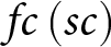 $fc\left( {sc} \right)$ is a non-linear function that determines the value of the worker’s contribution. Specifically, we allow
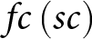 $fc\left( {sc} \right)$ to determine the value of workers’ contribution in a tax-progressive fashion, where the contribution rate is
 ${t_1}$ for the portion of contribution wages that is less than 1.5 minimum wages,
 ${t_2}$ for the range between 1.5 and 2.5 minimum wages, and
 ${t_3}$ for the remaining portion (up to the contributory wage cap), where
 ${t_1} \lt {t_2} \lt {t_3}$.
Generally, the calculation of the retirement benefit in a DB system considers a time window of the  $l$ last contribution wages of the worker. The average wage, which corresponds to these
 $l$ contribution wages, can then be expressed as:
 \begin{equation}s{m_{c,e,g}} = \left( {\mathop \sum \limits_{i - l \lt j \lt i} s{c_{c,e,g,j}}{p_{c,e,g,j}}} \right)\Bigg/\left( {\mathop \sum \limits_{i - l \lt j \lt i} {p_{c,e,g,j}}} \right).\end{equation}
As  $p$ is the probability of a contribution to the system, the accumulation of these probabilities provides the expected value of the number of contributions, or contributory density, of the agent up to age
 $i$, and is given by:
 \begin{equation}{n_{c,e,g,i}} = \mathop \sum \limits_{j \leqslant i} {p_{c,e,g,j}}.\end{equation}
2.3.3. Eligibility and benefit variables
Expressions (11) to (16) define the eligibility rules for regular retirement, the entitlement to the assistance benefit and express how the benefits of the systems are calculated. First, we define the retirement age for the group of workers who fulfil the rules for regular retirement, which are based on having reached both a minimum age and a minimum number of contributions to the system (expression (11)). Those who do not meet these conditions and who are poor are entitled to the assistance benefit, whose eligibility depends on a fixed minimum age and on whether the worker’s average wage is below the minimum wage. Agents who do not meet these criteria are granted the social benefit after a fixed age (expression (12)).
To calculate benefits in the notional DC system, we first specify how agents’ pension wealth accumulates over their working lives: whenever the agent contributes, this value accumulates in the agent’s pension wealth, which is remunerated by the rate of increase in productivity (equation (13)). The DC benefit itself is a perpetuity whose value depends on the agent’s accumulated wealth and the life expectancy of his/her birth cohort at retirement age (equation (15)). As for the value of the benefit in the DB system, it depends on the agent’s average wage at retirement age multiplied by a replacement rate formula that contains a term invariant to the agent’s contribution history and another term that is a fraction of the number of contributions (equation (14)). For both DC and DB schemes, the minimum value of the benefit is set at the minimum wage. As for the assistance benefit, its value equals the minimum wage (equation (16)). The construction of the eligibility and benefit variables is detailed below.Eligibility for retirement benefit is based on both a minimum age and a minimum number of contributions, both of which vary with the gender of the worker. Reflecting these conditions, the age at which the worker retires is then given by:
Regular retirement:
 \begin{equation}if\,\# \left( {{\Omega _{c,e,g}}} \right) \gt 0:{A_{c,e,g}} = \,{\text{min}}\left\{ {i \in {\Omega _{c,e,g}}} \right\},\end{equation}
where $\Omega {\,_{c,e,g}}\, = \,\left\{ {i:\,i \geqslant i0\left( g \right)\,\& \,{n_{c,e,g,i}} \geqslant n0\left( g \right)} \right\}$ and
 $i0\left( g \right)\,$and
 $n0\left( g \right)$ are respectively the parameters for the minimum age and the minimum number of contributions for gender
 $g$.
In many countries, including Brazil, social security systems include a component that guarantees a minimum benefit to those who, after a certain age, do not meet the criteria for retirement or have a (family) income less than a certain minimum value. Usually financed by general taxes, this benefit has an assistance character and aims to reduce the poverty of the elderly (Gill et al., Reference Gill, Packard and Yermo2005). In Brazil, it is called Benefício de Prestação Continuada (BPC – Continuous Cash Benefit) and grants a minimum wage to seniors aged 65 years and over whose per capita family income is less than one-fourth of the minimum wage. In our exercises, we assume that agents are entitled to receive this benefit when they do not meet the criteria for regular retirement expressed in (11), are aged 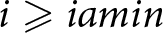 $i \geqslant iamin$ and have average wage
 $s{m_{c,e,g,i}} \lt smi{n_{c + i}}$ or, if these criteria are not met, start to receive the benefit at age
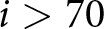 $i \gt 70$.Footnote 23 With these criteria, the age at which the assistance benefit is granted is expressed by:
Non-regular retirement:
 \begin{equation}if\,\# \left( {{\Omega _{c,e,g}}} \right) = 0:{A_{c,e,g}} = \,{\text{min}}\left\{ {\left\{ {i:\,i \geqslant iamin\,\& \,s{m_{c,e,g,i}} \lt smi{n_{c + i}}} \right\},\,70} \right\},\end{equation}
where  $iamin$ is the minimum age established in the social security system for granting this type of benefit.
Some simulations are based on the DC system with accumulation of notional assets by the worker. This asset is individual and is accumulated according to the contributions made by the worker and by the application of a remuneration rate that varies over time. Specifically, the expression for the agent’s notional asset at age  $i$ is given by:
 \begin{equation}{x_{c,e,g,i}} = \,\left[ {{x_{c,e,g,i - 1}}*\left( {1 + {y_{c + i}}} \right)} \right] + \left[ {v{c_{c,e,g,i}}*{p_{c,e,g,i}}} \right],\end{equation}
where we assume that the rate of remuneration is given by the variation in productivity expressed in (5), 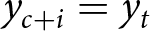 ${y_{c + i}} = {y_t}$, and the last term of the expression corresponds to the contribution when the worker contributes.Footnote 24
The amount of retirement benefits depends on whether the system is of a DB or DC type. In the former, the benefit is a function of the replacement rate over the agent’s average wage at retirement age. In DB systems, such as the one in Brazil, the replacement rate is formed by a constant component (differentiated by gender) and another variable component that corresponds to a fraction of the accumulation of contributions at the time of retirement. In the DC system, the benefit amount corresponds to a perpetuity calculated by the value of the asset accumulated by the agent divided by the life expectancy of the agent’s own cohort at the time of retirement. Both systems have a benefit floor for agents who do not meet the criteria for regular retirement. For groups that qualify for regular retirement – that is, those with 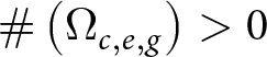 $\# \left( {{\Omega _{c,e,g}}} \right) \gt 0$ – the formulas for calculating the benefit,
 ${b_{c,e,g}}$, at age
 $i$ for each system are given by:
 \begin{equation}{\text{DB}}:\,{b_{c,e,g}}\, = \,max\left( {smi{n_{c + i}},\,s{m_{c,e,g,{A_{c,e,g}}}}*\left[ {\alpha \left( g \right) + \beta *{n_{c,e,g,{A_{c,e,g}}}}} \right]} \right)\end{equation}
 \begin{equation}\,{\text{DC}}:{\text{ }}\,{b_{c,e,g}} = \,max\left( {smi{n_{c + i}},\,{x_{c,e,g,{A_{c,e,g}}}}/v{e_{c,e,g,{A_{c,e,g}}}}} \right),\end{equation}
where  $\alpha \left( g \right)$e
 $\beta $ are the parameters of the replacement rate that represent the constant component (for gender g) and the fraction of the accumulation of contributions, respectively, and
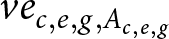 $v{e_{c,e,g,{A_{c,e,g}}}}$ is the life expectancy of the agent born in cohort
 $c$ and gender
 $g$ at retirement age
 ${A_{c,e,g}}$. For groups that do not qualify for regular retirement – that is, those with
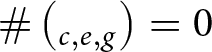 $\# \left( {_{c,e,g}} \right) = 0$, we have:
 \begin{equation}{\text{Assistance benefit}}:{ }{b_{c,e,g}} = smi{n_{c + {A_{c,e,g}}}},\end{equation}
where  ${A_{c,e,}}_g$ represents the minimum age at which the worker starts to receive this type of benefit.
Table 1 presents the parameters that condition the rules of the DB and DC systems of reference that we use in our simulations.
2.4. Outcome measures
In this subsection, we present a set of outcome measures for the simulations of the systems. First, we define variables at the agent level that allow us to answer questions about how the simulated systems affect the inequality of permanent income and the equity of rates of return between agents of the same cohort and between agents of different cohorts. Second, we construct variables to measure the deficit of the systems so that we can assess the aggregate impact of the simulated systems on their financial balance.
2.4.1. Outcomes per agent: income, inequity, and inequality
To summarize agents’ transactions with the PAYG system, we define a variable that measures in a cash-flow manner the contributions paid and benefits received by the agent before and after the age of eligibility for benefits (equation (17)). This variable is used to calculate the internal rate of return for heterogeneous agents (in terms of gender and education) of the same cohort (equation (20)) and for the representative agent of different cohorts (equation (21)). We use the standard deviation to measure the inequity in these rates of return.
For developing countries such as Brazil, the income of agents during their working life can be modeled as the combination of income in the formal sector (if they contribute to the pension system) and income in the informal sector (if they do not contribute). We model the average weighted income in the formal and informal sectors of the agent using as weights the probability of contributing to the pension system and the ratio of informal to formal income during the working life (equation (18)). Taking the present discounted value of this income stream gives the permanent income of agents during their working life, disregarding their contributions to the pension system (equation (19)). To assess the impact of the simulated systems on the inequality of permanent income between groups in the same cohort, we follow a series of steps. First, we define a variable (equation (22)) that measures the present discounted value of the income stream associated with agents’ relationship with the pension system (i.e., the previous cash flow variable of contributions paid and benefits received). Second, this variable is added to the permanent income of the agent without the pension system to obtain the permanent income of agents with a pension system. Finally, by subtracting the coefficient of variation of this resulting variable from the coefficient of variation of permanent income without the pension system, we obtain a measure of inequality in permanent income due to the pension system (equation (23)). The outcome variables at the agent level are presented in detail below.
Given the agent’s profile and the PAYG system rules, we can define a set of flow measures to compute outcome variables per agent. The flow measures are social security contributions and benefits as well as average income, which seek to incorporate the agent’s non-formal earnings throughout the life cycle. Viewed from a cash flow perspective, paid contributions and received benefits by the agent at age  $i$ are expressed by:
 \begin{equation}{f_{c,e,g,i}} = \left\{ {\begin{array}{*{20}{c}}
{ - v{c_{c,e,g,i}}\,\,\,\,\,\,\,\,\,\,\,{\text{se}}\,i \lt {A_{c,e,g}}\,{\text{(paid contributions)}}} \\
{{b_{c,e,g}}*p{s_{c,g,i}}\,{\text{se}}\,i \geqslant {A_{c,e,g}}\,{\text{(received benefits)}}}
\end{array}} \right.,\end{equation}
where 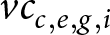 $v{c_{c,e,g,i}}$,
 ${b_{c,e,g}}$ and
 ${A_{c,e,g}}$ were defined in section 2.3 and
 $p{s_{c,g,i}}$ corresponds to the probability of survival of the agent of cohort
 $c$ and gender
 $g$ at age
 $i$. For a representative agent of cohort
 $c$, contributions and benefits at age
 $i$ can be expressed as a weighted average by gender and educational category as
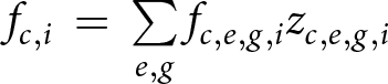 ${f_{c,i}}\, = \,\mathop \sum \limits_{e,g} {f_{c,e,g,i}}{z_{c,e,g,i}}$.
To compute a measure of the agent’s permanent income, it is important to take into account that in developing countries such as Brazil, workers have a high probability of spending periods of their life cycle with only non-formal income. To incorporate this dimension, we compute the income of agent 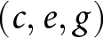 $\left( {c,e,g} \right)$ at age
 $i$ as a weighted average of formal and non-formal income, where the weight is the probability of contributing to social security,
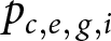 ${p_{c,e,\,g,i}}$. Specifically, average income is computed by:
 \begin{equation}{r_{c,e,g,i}} = {\text{exp}}\left( {{s_{c,e,g,i}}} \right)*\left( {{p_{c,e,g,i}}{\text{*}} + \left( {1 - {p_{c,e,g,i}}} \right)*x{f_{c,e,g,i}}} \right),\end{equation}
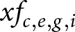
where 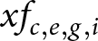 $x{f_{c,e,g,i}}$ is the predicted value of the ratio between non-formal income
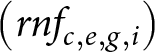
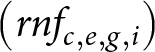 $\left( {rn{f_{c,e,g,i}}} \right)$ and formal income [
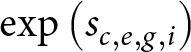 ${\text{exp}}\left( {{s_{c,e,g,i}}} \right)$].Footnote 25
Based on  ${f_{c,e,,i}}$ e
 ${r_{c,e,g,i}}$ defined in expressions (17) and (18), we calculate a set of outcome variables per agent. One of them is permanent income, which is given by the discounted income stream over the agent’s life cycle:
 \begin{equation}{R_{c,e,g}} = \mathop \sum \limits_i {r_{c,e,g}}p{s_{c,g,i}}{\left( {1 - \lambda } \right)^{ - i}},\end{equation}
where  $\lambda $ is a fixed discount rate.Footnote 26
Another measure is the internal rate of return ( $irr$) of the flow of paid contributions and received benefits, by a group of agents and for the representative agent:
 \begin{equation}{\rho _{c,e,g}} = irr\left( {{f_{c,e,g,i}}} \right)\end{equation}
 \begin{equation}{\rho _c} = irr\left( {{f_{c,i}}} \right),\end{equation}
where  ${\rho _c}$ is the aggregate rate of return for cohort
 $c$ (i.e., for the representative agent of cohort
 $c$).
To measure the inequity of rates of return between agents, we use the standard deviation ( ${\text{sd}}$) of these rates, namely:
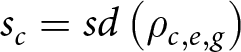 ${s_c} = sd\left( {{\rho _{c,e,g}}} \right)$ for educational groups and genders from the same cohort, and
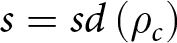 $s = sd\left( {{\rho _c}} \right)$ for the representative agents of different cohorts. We also compute a measure that seeks to assess the effect of pension systems on intragenerational permanent income inequality. To this end, we compute the present value of the contribution and benefit flows (including the assistance benefit):
 \begin{equation}\Delta {R_{c.e.g}} = \mathop \sum \limits_i {f_{c,e,g,i}}{\left( {1 - \lambda } \right)^{ - i}},\end{equation}
and define the measure of the systems’ effect on permanent income inequality for cohort  $c$ by the expression:
 \begin{equation}\Delta {\psi _c} = cv\left( {{R_{c,e,g}} + \Delta {R_{c.e.g}}} \right) - cv\left( {{R_{c,e,g}}} \right),\end{equation}
where  $cv\left( . \right)$ denotes the coefficient of variation. Note that the first term measures the level of inequality by incorporating the discounted flow from the pension system to permanent income, while the second term measures inequality from permanent income in a hypothetical situation where there is no pension system.
2.4.2. Aggregated outcomes per year: financial stability of PAYG systems
For a set of simulations, we use aggregated results per year to measure the financial stability of the systems. These measures are based on the revenues and expenditures of the system in period 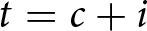 $t = c + i$, which are obtained by weighting the agent level variables by their proportion in the population. The revenue measure aggregates the contributions of all agents of all ages present at
 $t$, given by:
 \begin{equation}{R_t} = \mathop \sum \limits_{c,e,g} \mathop \sum \limits_{i \in I\left( {c,t} \right)} v{c_{c,e,g,i}}*{p_{c,e,g,i}}*{z_{c,e,g,i}}*po{p_{c,g,i}},\end{equation}
where all terms were defined in section 2.3. Expenditures on the payment of benefits (which include the assistance benefit) and the accumulated value of wage contributions are aggregated in a similar fashion:
 \begin{equation}{G_t} = \mathop \sum \limits_{c,e,g} \mathop \sum \limits_{i \in I\left( {c,t} \right)} {b_{c,e,g}}*p{s_{c,g,i}}*{z_{c,e,g,i}}*po{p_{c,g,i}}\end{equation}
 \begin{equation}fs{c_t} = \,\mathop \sum \limits_{c,e,g} \mathop \sum \limits_{i \in I\left( {c,t} \right)} s{c_{c,e,g,i}}*{z_{c,e,g,i}}*po{p_{c,g,i}}\end{equation}
The system deficit in period  $t$ is presented as the potential increase in the rate required to cancel the deficit, calculated by normalizing the deficit (
 ${G_t} - {R_t}$) with the potential tax base, i.e., the aggregate contribution salary:
 \begin{equation}{A_t} = \left( {{G_t} - {R_t}} \right)/fs{c_t}.\end{equation}
3. Results
The model described in Section 2 is simulated over the life cycle of agents aged  $i \in \left\{ {20, \ldots ,90} \right\}$ and born in cohort
 $c \in \left\{ {1942, \ldots ,2050} \right\}$, with the agent profile estimated up to the 1982 cohort and projected for the other cohorts. Therefore, in each year
 $t$, 70 cohorts live together, from those born in
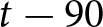 $t - 90$ to those born in
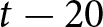 $t - 20$. The rules of the simulated systems are in effect from
 $t = 2016$ and, until this year, it is assumed that a stylized system (PAYG) is in force generating an initial state in 2015 with financial balance. In 2015, there is a contingent of agents who, if active, have a contributory history and, if inactive, are entitled to benefits calculated according to PAYG rules.Footnote 27 For these agents (specifically those of cohorts born up to 1994), revenues and expenditures are projected according to fixed rules that are different from those applied in the simulations.
The objective of the simulations is to relate types and designs of PAYG structures – which we will generically call rules – with the aggregate financial imbalance of the system, permanent income inequality and the rate of return of social security assets of agents from different groups and cohorts. Interpreting the effects of rules on the trajectory of the outcome variables of interest is a difficult task because the relationships are complex in themselves, the agents’ profiles have long-term trends and are inserted in PAYG schemes in which part of the contribution rate is progressive. Furthermore, the rules and the adjustments required to financially balance the systems affect groups of agents in a heterogeneous way and there is an assistance pillar that introduces discontinuities in the results. Thus, to facilitate understanding of the effects of the different rules, results are presented in three subsections. In the first one, we discuss different rules that determine the value of the benefit in a stylized environment in which some components of the system are excluded to allow a more direct evaluation of effects. In the second subsection, the system is re-evaluated in a more realistic environment where the excluded components are reintroduced. In both subsections, financial imbalances are allowed over time, that is, it is implicitly assumed that there are external sources to the system that guarantee its sustainability. In the third subsection, the financial imbalance is eliminated within the system through the introduction of alternative rules that require adjustment contributions from active and inactive groups. The introduction of these adjustment contributions alters the flow of payments and receipts of the agents and, therefore, differently affects inequality and returns for different groups of agents born in different cohorts.
The last projected cohort ( $c$=2050) enters the labor market in 2070 and generates a flow of resources until 2140. Assuming that cohorts after 2050 have the same profile as the last cohort, revenue and expenditure streams were generated until 2140. Therefore, in 2080 we have the year for which the hypotheses for the projection are fully computed and the subsequent years show the trends of revenues and expenditures relative to the last projected cohort. In summary, the initial period of the projection is 2016, the terminal is 2080, and from there until 2140, only the trends implicit in the hypotheses operate.
Before presenting the results of the simulations, it is worth discussing some of the main forces that affect the outcome variables. The projection hypotheses that make wages, the probability of contribution, and education grow across newer cohorts imply that the distributions of these variables will be shifting to the right over the years. These movements, which implicitly reflect the process of development in the long term, have important implications for our results. First, they imply that workers will be less concentrated at the bottom of the wage distribution and, as a result, less dependent on the benefit floor and the assistance benefit. Second, as we keep the value of the minimum wage constant, given that it conditions the tax-progressive contribution ranges of wages (including the contributory wage cap), there will be higher concentration of workers along the upper ranges, which endogenously increases the effective contribution rate and diminish the rate of return of these groups of workers. The fixed value of the minimum wage also affects disbursements with the benefit floor and the assistance benefit which, together with the systematic decrease in concentration of dependents of the minimum wage, produce deficit reductions. Another force in operation is the increase in the dependency ratio, which systematically reduces the proportion of active workers and increases that of the inactive. Clearly, this force increases the expenses of the systems with all types of benefits (including the assistance benefit), reduces the revenues of the systems, and for the case of financially balanced structures, increases the burden on the active and inactive groups to balance the systems. These forces will be in operation in a complex way, and we now turn to the simulation results to unveil their final effects on the outcome variables.
3.1. Unbalanced systems without pension floor and assistance benefit
To highlight the relationship between rules and results more directly, we consider in this section stylized PAYG structures in which two components of the system that generate non-trivial discontinuities on results are excluded, namely: (i) the minimum amount for the retirement benefit and (ii) the guarantee of assistance benefits for the elderly poor.
In the DB system in force in Brazil, the benefit amount is calculated based on a replacement rate that is the sum of two components: 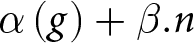 $\alpha \left( g \right) + \beta .n$, where the first, which varies by gender, does not depend on the number of contributions made until retirement (
 $n$) and can be seen as a compensation for groups that have lower contributory densities such as women and informal or self-employed workers. To isolate the effect of these components, we consider four alternative scenarios for computing the retirement benefit amount. Specifically, using the notation from Section 2.3 (without the subscripts), the simulated systems areFootnote 28:
 \begin{equation}{\text{na}}1){\text{ DB}}\_{\text{NA}}:\alpha \left( g \right)sm + \beta.n.sm;\end{equation}
 \begin{equation}{\text{na}}2){\text{ DB}}\_{\text{NA}}0:{ }\beta .n.sm;\end{equation}
 \begin{equation}{\text{na}}3){\text{ DC}}\_{\text{NA}}:{ }x/ve;\end{equation}
 \begin{equation}{\text{na}}4){\text{ DM}}\_{\text{NA}}:\,\alpha \left( g \right)sm + x/ve.\end{equation}
The DB_NA system corresponds to the DB system in use in Brazil – i.e., expression (15) without the benefit floor. The DB_NA0 scenario is a variant of DB_NA in which the compensation that is independent of the contributory density of the agent is eliminated. The DC_NA system corresponds to the benefit of the notional DC system – i.e., expression (16) without the benefit floor – in which the agent receives the capitalization of what he/she contributed ( $x$) divided by the expected life (
 $ve$). And, finally, the DM_NA system is a new mixed system that adds to the benefit of the DC system, the compensation that is independent of the contributory density of the DB system.Footnote 29 Systems DB_NA0 and DC_NA contain only the component that depends on the contributory density and differ from each other by computing the effect of this density differently. Similarly, systems DB_NA and DM_NA incorporate the compensation component independent of the contributory density and differ from each other for the same reason as in the previous pair of cases.
In Figure 1, graphs 1.a, 1.b, and 1.c present the simulation results of these four systems respectively for the aggregate deficit ( ${A_t}$), the effect on permanent income inequality (
 $\Delta {\psi _c}$) and the rate of return for the representative agent (
 ${\rho _c}$). Graphs 1.d to 1.g (1.h to 1.k) show the rates of return of men (women) for different educational groups (
 ${\rho _{c,e,g}}$). Due to the similarity of the results for some educational groups, to simplify the presentation, the rates of return of the groups (
 $e = 1,\,e = 2$) and of (
 $e = 3,\,e = 4$) were aggregated using as weight the proportion of agents with these educational levels in each cohort over time. In all graphs of this and other sections,
 $t = 2016,\ldots.,2080$ and
 $c = 1980,\ldots,2040$.
Simulation results for unbalanced systems without pension floor and assistance benefit.
Note: The graphs are: 1.a: Deficit per year,  ${A_t}$; 1.b: Effect on permanent income inequality between groups by cohort,
 $\Delta {\psi _c}$; 1.c: Aggregate rate of return by cohort,
 ${\rho _c}$. The other graphs refer to the rate of return by cohort, educational group, and gender,
 ${\rho _{c,e,g}}$, as indicated in the figure. The lines correspond to the benefit rules detailed in the text, where: DB_NA: defined benefit system (DB); DB_NA0: the restricted variant of DB_NA; DC_NA: notional DC system; and md0: mixed system that combines components from the DC and DB systems.
Source: Simulations based on data from Pesquisa Nacional por Amostra de Domicílios (PNAD).

Graphs 1.a, 1.b., and 1.c show that, while the pure DC system DC_NA has the smallest deficit, the smallest effect (in absolute terms) on permanent income inequality and the smallest rate of return, the pure DB system DB_NA exhibits the opposite pattern. In particular, it should be noted that the DB rate of return is more than three times higher than that of the DC and well above productivity growth, which is an indicator of future deficits in the system.Footnote 30 The differences between the rates of return of the DB and DC systems are accentuated for the groups with lower education (graphs 1.d to 1.k), especially in the case of women, whose term of the replacement rate that does not depend on the contribution density is higher than that of men.Footnote 31 These differences between the two systems were expected as the DC system is, by design, more neutral, while the DB tends to be more generous, especially to the less skilled and to women.
Graphs 1.a to 1.c also show that the mixed system DM_NA, as well as the DB_NA0 system, present intermediate results between the DB and DC systems for deficit, permanent income inequality and rate of return. This intermediate pattern of the DM_NA and DB_NA0 systems is also observed for the returns of the educational groups, both for men (graphs 1.d–1.g) and for women (graphs 1.h–1.k). However, the DM_NA system tends to present higher returns for groups with less education, especially for women, which is explained by the presence of the term that is independent of contributory density in the calculation of the benefits of the DM_NA system. It is also interesting to note that the rates of return are higher for women than for men for almost all systems, the exception being the DC structure DC_NA, which displays a neutral return across the board.
Except for the case of the DC structure DC_NA, it is interesting to note that the deficits of all other systems tend to increase in the long run with positive values even in the context without pension floor and assistance benefit. This results from the combination of some operating forces that were discussed before. Clearly, the rise in the dependency ratio operates as a deficit enhancer. But the systematic increase in the probability of contributions to social security and the rise in effective tax rates paid by workers – due to the shifts to the right of the distributions of wages and education – are deficit reducers. There are also the opposing effects associated with the presence of the fixed wage contribution cap: on one hand, it limits the total value of contributions but, on the other, it also creates a cap on benefit payment. The results in graph 1.a show that the deficit reducers were not strong enough to counterbalance the effects of the deficit enhancers.
As for the effects on inequality of permanent income and the rates of return (graphs 1.b and 1.c, respectively), we see that they tend to be relatively stable across almost all cohorts (except for the first ones) for all systems. However, this is not observed for the rate of return of the DB system DB_NA for the more educated groups workers (especially males), which indicates that the rise in the effective contribution rate tends to depress the return for these groups in that system.
It is also possible to observe in graphs 1.a to 1.c that the aggregated results of the DM_NA and DB_NA0 systems are similar. Though subject to the parameterization used, this similarity of results implicitly confirms the generosity of the DB system. The mixed system DM_NA can be seen as a DC system in which a compensation is introduced for groups with the lowest propensity to contribute – specifically, the term that is independent of contributory density in the DB system. The incorporation of this component in the DM_NA system makes its results similar to those of the DB_NA0 system, which, like the DC system, does not have this compensation component.
These results motivate the evaluation of the functioning of the mixed system DM_NA, which reduces the deficit compared to the DB system, has a greater inequality-reducing effect than the DC system and presents an intermediate rate of return between the DB and the DC, including for the different educational groups and genders. However, the abrupt change from the initial DB system to the DM_NA mixed system has the inconvenience of generating a discontinuity in the value of the benefit. For this reason, we propose an adjustment of the rule in which the benefit starts from the DB system and converges in a certain number of years to the mixed system DM_NA. More specifically, the benefit formula in this system (which we denominate DM) is given by:
 \begin{equation}{\text{s}}5){\text{ DM}}:{ }\alpha \left( g \right)\,sm\, + \,\left[ {\gamma \left( {\beta *n} \right)sm + \,\left( {1 - \,\gamma } \right)\,x/ve} \right],\end{equation}
where  $\gamma = {\text{max}}\left\{ {0,1 - \Delta \gamma \,\left( {t - t0} \right)} \right\}$ is the function that regulates the transition phase. Unless stated otherwise, in the simulations of this system, we set
 $\Delta \gamma = 0.025$ and
 $t0 = 2016$.Footnote 32
3.2. Unbalanced systems with pension floor and assistance benefit
In this section, we evaluate the functioning of the DB, DC, and the new mixed DM system presented in the previous subsection in a more realistic environment where the existence of the minimum benefit amount and the guarantee of the assistance benefit for the elderly poor are incorporated.
wa1) DC_WA: DC system with benefit calculated by expression (15);
wa2) DM_WA: DM system with benefit calculated by expression (32);
wa3) DM_WA_IT: DM system with instantaneous transition (i.e., with $\gamma = 0$ in expression (32));
wa4) DB_WA: DB system with benefit calculated by expression (14).
In Figure 2, graphs 2.a, 2.b, 2.c show several results that are worth noting. First, it is possible to observe that the incorporation of the social security floor and the guarantee of minimum benefit for the elderly poor do not qualitatively change the comparisons between the DC, DB and DM systems discussed in the previous subsection. The DM system (DM_WA and DM_WA_IT) remains an intermediary scheme between the DB (DB_WA) and the DC (DC_WA) systems for almost all variables, the only exception being the effect on inequality in the latter system (see below).
Simulation results for unbalanced systems with pension floor and assistance benefit.
Notes: The graphs are: 2.a: Deficit per year,  ${A_t}$; 1.b: Effect on permanent income inequality between groups by cohort,
 $\Delta {\psi _c}$; 1.c: Aggregate rate of return by cohort,
 ${\rho _c}$. The other graphs refer to the rate of return by cohort, educational group, and gender,
 ${\rho _{c,e,g}}$, as indicated in the figure. The lines correspond to the benefit rules detailed in the text, where: DB_WA: defined benefit system (DB); DC_WA: notional defined contribution (DC) system; DM_WA: mixed system (DM) that combines components from DC and DB systems and has a smooth transition (
 $\Delta \gamma = 0.025$); and DM_WA_IT: mixed system (DM) with instantaneous transition (
 $\gamma = 0$).
Source: Simulations based on data from Pesquisa Nacional por Amostra de Domicílios (PNAD).

Secondly, differently from the previous subsection, some trends clearly appear in the outcome variables for all systems. As aforementioned, it is difficult to disentangle the effects of each operating factor but it is clear that the introduction of the benefit floor and the assistance benefit is generating the trends. This is particularly noticeable for the DC_WA system, a result that shows that even a neutral structure like the notional DC can be strongly affected by the insertion of restrictions on benefit floors and assistance benefits.Footnote 33
Compared to the context without pension floor and assistance benefit (graph 1.a), the results of graph 2.a. reveal a rise in the deficit for all simulated rules, with the DB system DB_WA displaying the largest increase, the DC system DC_WA the smallest, and the proposed mixed system DM_WA an intermediate value. Graph 2.a also reveals that the incorporation of a transition phase from the DB system to the DM system DM_WA generates only a transient impact on the deficit compared to the system without transition (DM_WA_IT). This result is interesting as it shows that it is possible to modulate the effect on the deficit of a transition from the DB system to a mixed system in which the benefit calculation includes a component that is independent of contributory density and another component entirely based on systems of defined contribution.Footnote 34
The results in Graph 2.b show that the DC DC_WA system promotes a significant drop in permanent income inequality for the initial cohorts, but that this reduction gradually attenuates across the cohorts. This is because this system drastically reduces the benefits, leading to a high proportion of agents receiving the benefit floor, which substantially reduces inequality for the initial generations. The attenuation of the effect on inequality is mainly due to the shifts to the right of the distributions of wages, contributions and education, which decrease the proportion of groups restricted by the benefit floor. Graph 2.b also shows that the DB scheme DB_WA is the one that promotes the greatest reduction in inequality among cohorts. The reduction of inequality by the mixed systems DM_WA and DM_WA_IT is smaller (in module) than that of DB system, and the introduction of the transition between systems (DM_WA) has practically no effect on inequality. Unlike the trajectory of the DC scheme DC_WA, the DM_WA and DM_WA_IT systems do not present a concentration of groups that receive the benefit floor and that, as in the DC system, are particularly affected by the shift to the right of distributions of wages, contributions, and education.
In terms of ranking between systems, the rate of return of the representative agent presented in graph 2.c shows qualitatively similar results to those of section 3.1, that is, the DB presents a higher rate than that of the DM which, in turn, exhibits a higher rate than that of the DC. It can also be noted in graph 2.c that the difference in return between the mixed systems with and without transition (DM_WA and DM_WA_IT, respectively) is eliminated along the initial cohorts, which shows that with the transition the return converges smoothly to its long-term trend.
The sets of graphs 2.d to 2.g and 2.h to 2.k respectively show decreasing trends in the intergenerational return for men and women, especially for groups with lower education. The comparison of these graphs with the ones in the previous subsection confirms, for most systems and educational groups by gender, the downward effect of introducing additional restrictions due to the benefit floor and the assistance benefit. It is also notable that the introduction of these restrictions increases the rate of return for the lowest education groups, especially for females. In fact, as before, the rates of return for women are higher than those for men for almost all systems, except for the DC structure DC_WA for the most educated group, which displays equal return between the genders. As in the aggregate case, it is also noted that the difference in return between the mixed systems with and without transition (DM_WA and DM_WA_IT) disappears for initial cohorts of more educated groups – and it does not even show up for the least educated ones.
All simulations presented until this section assume that the deficit is financed by an external source that does not impact the agents’ returns. This makes the simulation results not strictly comparable. For example, as we have seen, the DB system generates greater returns than the mixed DM system, but its deficit is much higher. The next section introduces rules for adjusting the contributions of active and inactive groups to make all systems financially sustainable and, in that sense, more comparable.
3.3. Balanced systems with pension floor and assistance benefit
In a financially balanced pension system, revenues and expenditures are equal over the years and, to ensure this equality within the systems, active and inactive generations contribute to a fund that finances imbalances. The additional contribution of the active is a proportion of the contribution wage ( ${\tau _t}$) and the contribution of the inactive is a rate (
 $\tau {b_t}$) of the benefit received. It is assumed that active and inactive agents who respectively receive more than
 $L$ and
 $Lb$ multiples of the minimum wage contribute to this fund, that is, agents with lower income are excluded from the adjustment contribution. The rates of active and inactive groups are determined per year according to two classes of rules inspired in Auerbach and Lee (Reference Auerbach and Lee2011), namely:
 $A(\alpha )$: defines rates
 ${\tau _t}$ and
 $\tau {b_t}$ so that the proportion of the deficit paid by the inactive generations is equal to
 $\alpha $; and,
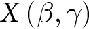 $X\left( {\beta ,\gamma } \right)$: defines the contribution rate of inactive generations,
 $\tau {b_t}$, according to expression (36) below and calculates the contribution rate of active generations,
 ${\tau _t}$, in a residual way to cancel the deficit (expression (37)).
The first class of rules distributes the adjustment burden between active and inactive groups according to a single policy parameter  $\left( \alpha \right)$ and has the advantage of controlling a relevant dimension, which is the relative burden between the two groups. The second class of rules is a stylized form of the system in use in Germany, where the contribution of the inactive is adjusted both by the variation of the ratio between the size of the inactive and the active population and by the variation in gross wages. In this rule, the inactive can be seen as a partner of the social security system, contributing more if the elderly population proportionally increases and contributing less (may be even with negative rates) when the wages increase. That is, the inactive generations have the system’s burden and bonus, and the active generations pay what is necessary to eliminate the deficit. Using the notation from section 2.3, the following equations define aggregate variables that are used in the two classes of adjustment rules. Let:
 \begin{equation}f{a_t} = \,\mathop {{\sum _{c,e,g}}}\limits_{} \mathop {{\sum _{i \in I\left( {c,t} \right)}}}\limits_{} I(s{c_{c,e,g,i}},L*smi{n_t})*{z_{c,e,g,i}}*po{p_{c,i,g}}\,{\text{and}}\end{equation}
 \begin{equation}f{b_t} = \,\mathop {{\sum _{e,g,c}}\ {\sum _{i \gt A\left( {c,e,g} \right)\mathop \cap \nolimits^ i \in I\left( {c,t} \right)}}}\limits_{} I({b_{c,e,g}},Lb*smi{n_t})*{z_{c,e,g,i}}*po{p_{c,i,g}},\end{equation}
where 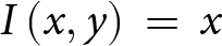 $I\left( {x,y} \right)\, = \,x$ if
 $x \geqslant y$ and
 $0$ otherwise,
 $sc$ is the contribution wage,
 $b$ is the benefit,
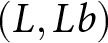 $\left( {L,Lb} \right)$ are the thresholds below which active and inactive do not contribute to balance the systems, and
 $smin$ is the minimum wage. Quantities
 $f{a_t}$ and
 $f{b_t}$ represent, respectively, the total funds arising from wages of the active and benefits of the inactive that are subject to the contribution to financially balance the system in period
 $t$.
Adjustment rule  $A(\alpha )$:
 \begin{equation}{\tau _t} = \left( {1 - \alpha } \right)\!.\, x_{t}{\text{ and }}\tau {b_t} = \alpha .\,x_t\end{equation}
where  ${x_t} = \left[ {{G_t} - {R_t}} \right]/\left[ {\left( {1 - \alpha } \right)\!.\,f{a_t} + \alpha .\,f{b_t}} \right]$.
Adjustment rule 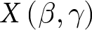 $X\left( {\beta ,\gamma } \right)$:
 \begin{equation}\tau {b_t} = 1 + (\tau {b_{t - 1}} - 1)*\left[ {\gamma \Delta s{l_t} - \beta \Delta r{d_t}} \right],\end{equation}
where:
 $\Delta r{d_t} = r{d_t} - r{d_{t - 1}}$: rate of increase in the ratio between the number of inactive and active (old-age dependency ratio);
 $\Delta s{l_t} = s{l_t} - s{l_{t - 1}}$: rate of increase in average gross wage,
and
 \begin{equation}{\tau _t} = \left[ {{G_t} - {R_t} - \left( {\tau {b_t}*f{b_t}} \right)} \right]/f{a_t}.\end{equation}
Applying these rules, contributions paid and benefits received by the agent 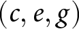 $\left( {c,e,g} \right)$ who contributes to the adjustment at age
 $i$ are expressed in a cash flow manner by:
 \begin{equation}{f_{c,e,g,i}} = \left\{ {\begin{array}{*{20}{c}}
{ - v{c_{c,e,g,i}}{ - \,_{c + i}}*I\left( {s{c_{c,e,g,i}},L*smi{n_{c + i}}} \right)\,\,\,\,\,\,\,\,\,\,\,\,\,\,\,\,\,{\text{if}}\,i \lt {A_{c,e,g}}\,} \\
{\left[ {{b_{c,e,g}}\, - \,{b_{c + i}}*I\left( {{b_{c,e,g}},Lb*smi{n_{c + i}}} \right)} \right]*p{s_{c,g,i}}{\text{ if}}\,i \geqslant {A_{c,e,g}}\,}
\end{array}} \right..\end{equation}
where 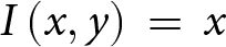 $I\left( {x,y} \right)\, = \,x$ if
 $x \geqslant y$ and
 $0$ otherwise,
 $vc$ is the contribution value based on the contribution wage,
 $b$ is the benefit,
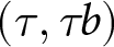 $\left( {\tau ,\tau b} \right)$ are the additional rates of contribution to balance the systems from the active and inactive, respectively
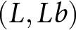 $\left( {L,Lb} \right)$, are the thresholds below which active and inactive do not contribute to balance the systems,
 $smin$ is the minimum wage, and
 $ps$ is the survival probability.
Simulations were chosen following the strategy of comparing DB and DM systems in different situations. For rule  $A\left( \alpha \right)$, we define a set of simulations assuming that active generations finance the entire deficit (i.e.,
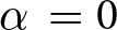 $\alpha \, = 0$) or that they share the burden in equal proportion with the inactive generation (i.e.,
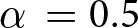 $\alpha \, = 0.5$). For the
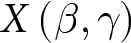 $X\left( {\beta ,\gamma } \right)$ rule, we use the parameterization
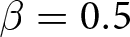 $\beta = 0.5$ and
 $\gamma = 1$, which implies that the inactive receive the entire wage gains and contribute half of the increase in the dependency ratio. In all cases, parameters
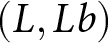 $\left( {L,Lb} \right)$ are fixed in
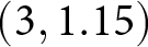 $\left( {3,1.15} \right)$.Footnote 35
The rules determine for each year the contribution rates of active and inactive generations alive in year  $t$ and, as they fluctuate over time, cause the agents of different cohorts to be heterogeneously affected. The simulated rules are:
wab1) DB_WA_B0: DB system with adjustment  $A\left( 0 \right)$ (i.e.,
 $\tau {b_t} = 0,\forall t$);
wab2) DM_WA_B0: DM system with adjustment  $A\left( 0 \right)$ (i.e.,
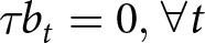 $\tau {b_t} = 0,\forall t$);
wab3) DB_WA_B5: DB system with adjustment 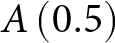 $A\left( {0.5} \right)$ (i.e.,
 $\tau {b_t}{ = _t}$);
wab4) DM_WA_B5: DM system with adjustment 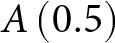 $A\left( {0.5} \right)$ (i.e.,
 $\tau {b_t}{ = _t}$);
wab5) DB_WA_BX: DB system where the rate of the inactive group is given by 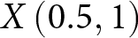 $X\left( {0.5,1} \right)$ and residual balance is provided by the active group;
wab6) DM_WA_BX: DM system where the rate of the inactive group is given by 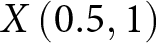 $X\left( {0.5,1} \right)$ and residual balance is provided by the active group.
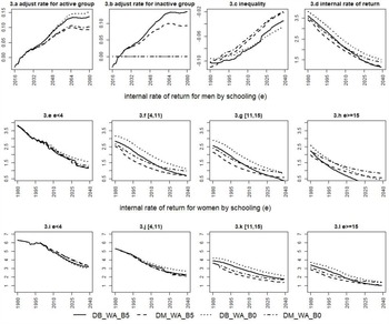
Figures 3 and 4 present results for two subsets of these rules in balanced systems where the deficit is zero. The graphs of these figures are similar to the previous ones, except for the pairs (3.a, 4.a) and (3.b, 4.b), which respectively present the value of the rates ( ${\tau _t},\tau {b_t}$) that are required from active and inactive groups to eliminate the deficit.
Simulation results for balanced systems with pension floor and assistance benefit – a rules.
Notes: The graphs refer to: 3.a: Adjustment rate of the active group per year,  ${\tau _t}$; 3.b: Adjustment rate of the inactive group per year,
 $\tau {b_t}$; 3.c: Effect on permanent income inequality between groups by cohort,
 $\Delta {\psi _c}$; 3.d: Aggregate rate of return by cohort,
 ${\rho _c}$. The other graphs refer to the rate of return by cohort, educational group, and gender,
 ${\rho _{c,e,g}}$, as indicated in the figure. The lines correspond to the benefit rules detailed in the text, where: DB_WA_B0: DB system with adjustment
 $A\left( 0 \right)$; DM_WA_B0: DM system with adjustment
 $A\left( 0 \right)$; DB_WA_B5: DB system with adjustment
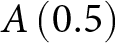 $A\left( {0.5} \right)$; and DM_WA_B5: DM system with adjustment
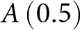 $A\left( {0.5} \right)$.
Source: simulations based on data from pesquisa nacional por amostra de domicílios (PNAD).

Simulation results for balanced systems with pension floor and assistance benefit – a and x rules.
Notes: The graphs refer to: 4.a: Adjustment rate for the active group per year,  ${\tau _t}$; 4.b: Adjustment rate for the inactive group per year,
 $\tau {b_t}$; 4.c: Effect on permanent income inequality between groups by cohort,
 $\Delta {\psi _c}$; 4.d: Aggregate rate of return by cohort,
 ${\rho _c}$. The other graphs refer to the rate of return by cohort, educational group, and gender,
 ${\rho _{c,e,g}}$, as indicated in the figure. The lines correspond to the benefit rules detailed in the text, where: DB_WA_B5: DB system with adjustment
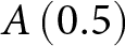 $A\left( {0.5} \right)$; DM_WA_B5: DM system with adjustment
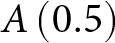 $A\left( {0.5} \right)$; DB_WA_BX: DB system with adjustment
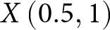 $X\left( {0.5,1} \right)$; and DM_WA_BX: DM system with adjustment
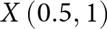 $X\left( {0.5,1} \right)$.
Source: Simulations based on data from Pesquisa Nacional por Amostra de Domicílios (PNAD).

Graph 3.a shows that DB systems DB_WA_B0 and DB_WA_B5 require higher contribution rates from the active group than DM systems DM_WA_B0 and DM_WA_B5. This difference between the systems can also be observed in graph 3.b for the rules involving the contribution of inactive generations, i.e., the DB_WA_B5 rule compared to DM_WA_B5. These results are consistent with the difference in deficits presented in sections 3.1 and 3.2 between these two types of systems.
The fund that finances the imbalances of the systems is based on the total contribution of active (inactive) groups,  $f{a_t}$ (
 $f{b_t}$), who receive more than
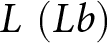 $L\,\left( {Lb} \right)$ minimum wages. In general, the
 $f{a_t}$ portion of the total fund is substantially larger than the portion, even taking into account the population aging process. This difference explains the proximity of the rates of the pair of rules DB_WA_B5 and DB_WA_B0 and, especially, of the pair DM_WA_B5 and DM_WA_B0 (graph 3.a). One implication of this result is to reveal a potential limitation of the
 $A\left( \alpha \right)$ rule, since the contribution of inactive generations does not generate a significant reduction in taxation on active workers even when the distribution of imbalances is carried out in a proportional way, i.e., with
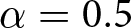 $\alpha = 0.5$.
As can be seen in Figure 3.c, all rules generate a reduction in permanent income inequality. However, this graph also shows that all rules display pronounced trends that attenuate across cohorts. This pattern is essentially due to two factors acting in opposite directions. On the one hand, the increase in the contribution of active and inactive agents observed in graphs 3.a and 3.b raises the proportion of agents who receive the minimum wage and this accumulation of agents at the minimum generates a reducing effect on inequality. On the other hand, shifts to the right in the distribution of wages, contributions, and education work to reduce the concentration of agents receiving the minimum. The trends observed in graph 3.c show that this second effect more than offsets the first effect across generations.
Another point to be observed in graph 3.c is that the DB system tends to reduce inequality more than the DM system. However, both systems show similar trends across cohorts. In fact, maintaining the trends observed in graph 3.c, the effect of the two types of systems tends to disappear for the last cohorts, with the difference that this occurs for later generations in the DB system than in the DM system.
Graph 3.d reveals that all rules show a downward trend in aggregate return across cohorts, with the rate of return converging towards the unit value in most rules for the final cohorts.Footnote 36 Another point to be highlighted in graph 3.d is a pronounced accentuation of the downward trends of the DB and DM systems comparable to those analyzed in section 3.2 (graph 2.c) – specifically DB_WA for the DB case and DM_WA for the DM case. In other words, the introduction of the contribution of active and inactive generations to eliminate the growing deficits of the DB and DM systems (as shown in graph 2.a.) intensifies the downward trends in the representative agent’s return already observed in the context without financial equilibrium. It is also noticeable in graph 3.d that the rules that tax the inactive in the same type of system have a systematically lower return than those that do not tax them (i.e., DB_WA_B5 compared to DB_WA_B0 or DM_WA_B5 compared to DM_WA_B0). These patterns in rates of return are also verified for almost all educational groups of both men (graphs 3.e to 3.h) and women (graphs 3.i to 3.l).Footnote 37 These results show that the rate of return is strongly influenced not only by increases in the taxation of the active generations, but also by the adjustment contribution of the inactive ones. The comparison of the rates of return of males and females shows that the introduction of adjustment contributions on the active and inactive groups does not change the previous result that the latter group has higher rates than the former.
We selected rules DB_WA_B5 and DM_WA_B5 to compare with rules DB_WA_BX and DM_WA_BX, which are based respectively on a DB and a DM system whose benefits are affected by changes in both the dependency ratio and gross wages. The results are shown in Figure 4, whose graphs are arranged in the same way as in Figure 3.
The simulations in Figure 4 make it possible to compare the rules 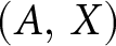 $\left( {A,\,X} \right)$ and the systems (DB, DM), that is, they allow the analysis of the partial effects of changing the adjustment rule given the system – i.e., comparing DB_WA_B5 with x2b or DM_WA_B5 with x2m – or from changing the system given the adjustment rule – i.e., comparing DB_WA_B5 with DM_WA_B5 or x2b with x2m. Graph 4.a shows that the adjustment rules DB_WA_BX and DM_WA_BX display lower contribution rates from the active group than their counterparts in rule
 $A$, DB_WA_B5 and DM_WA_B5 respectively. This result indicates that the class of rules that modulate benefits based on the dependency ratio and the evolution of wages lessens the additional taxation that falls on active generations. Graph 4.a also shows that system DB (DB_WA_B5 and DB_WA_BX) exhibits higher rates than their MD counterparts (DM_WA_B5 and DM_WA_BX, respectively).
Looking at the contribution rates of the inactive group, graph 4.b evinces that the DB system combined with rule  $A$ (DB_WA_B5) taxes a higher rate from this group than the MD system with the same rule (DM_WA_B5). Thus, in the case of adjustment rule
 $A$, the DB system has a higher tax burden on both the active and the inactive generations than the MD system. By construction, the inactive group is charged in the same way by rule
 $X$ for both the DB (DB_WA_BX) and the MD (DM_WA_BX) systems. Interestingly, as displayed in graph 4.b, the contribution rate of the inactive for this rule has an inverted-U shape, showing that the force of the variation in wages is capable to surpass that of the dependency ratio for the later period. This shape makes the curve of the
 $X$ rule to cross from above the curves of the
 $A$ rule (DB_WA_B5 and DM_WA_B5), which implies that the burden on the inactive group to help balancing the system is only smaller in the former rule than for the latter at the end of the period of analysis.
As can be seen in graph 4.c, the effects on inequality of rule  $X$ (DB_WA_BX and DM_WA_BX) are very similar to their counterparts in rule
 $A$ (DB_WA_B5 and DM_WA_B5, respectively). Graph 3.c also shows that rules based on the DB system (DB_WA_B5 and DB_WA_BX) have a systematically greater effect (in module) than rules based on the DM system (DM_WA_B5 and DM_WA_BX). As before (see graph 3.c), the main difference between these two systems is that relative to the DM scheme, the effect tends to cancel out for the DB system for later cohorts.
In graph 4.d, it is possible to see that rule  $X$ (DB_WA_BX and DM_WA_BX) presents the same pattern of falling return for the representative agent as rule
 $A$ (DB_WA_B5 and DM_WA_B5). This result confirms what was mentioned earlier about the compressing effect that the introduction of contributions of active and inactive generations has on the representative agent’s return. It is observed, however, that rule
 $X$ exhibits greater returns than rule
 $A$ both for the DB system (DB_WA_BX compared to DB_WA_B5) and for the DM system (DM_WA_BX compared to DM_WA_B5). This result indicates that the rate of return of the class of rules that adjusts benefits according to the evolution of demographics and wages tends be higher than that based on the proportional distribution of the burden between active and inactive groups. Keeping the rules fixed, graph 4.d also shows that the rates of return are higher for the DB system (DB_WA_B5 and DB_WA_BX) than their counterparts in system MD (DM_WA_B5 and DM_WA_BX, respectively).
As can be seen in graphs 4.e to 4.h and 4.i to 4.l, except for the group of women with less education, the other educational groups of both sexes experience a pattern of decline in returns similar to that of the representative agent. It is also possible to see in these graphs the higher returns of the  $X$ rules in relation to their corresponding
 $A$ rules for educational groups of both sexes. These results indicate that rule
 $X$ can generate greater returns to agents than rule
 $A$ across cohorts. Notwithstanding the downward trend in returns for both genders, as before females have higher rates of return than those of males.
Finally, to assess the impacts of the balanced systems on intergenerational equity, Table 2 presents the standard deviation of rates of return between cohorts for both the representative agent and different educational groups by gender. As seen earlier, these rates of return show downward trends, but even in this situation, this measure can capture the differences in return inequality between systems. Table 2 shows that, in general, the simulation of the DM system with rule  $X$ (i.e., DM_WA_BX) is the one with the smallest dispersion, while the simulation of the DB system with rule
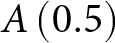 $A\left( {0.5} \right)$ (i.e., DB_WA_B5) is the one with the greatest dispersion. The other rules/systems constitute intermediate cases, but with a tendency for those based on rule
 $A$ and system
 $DB$ to exhibit higher intergenerational inequity. It is interesting to note that the systems/rules with the lowest (highest) standard deviation tend to require the lowest (highest) taxation on the active group. One explanation for this pattern is that adjustments made earlier in the life cycle are less discounted than those that occur later (Auerbach and Lee, Reference Auerbach and Lee2011). It is also interesting to note that intergenerational inequality in returns is higher for females than for males in all education groups.
Standard deviation of the rate of return across cohorts by gender and education group

Notes: The systems/rules are detailed in the text and summarized in appendix C. Bold (underlined) numbers indicate the lowest (largest) standard deviation for each column in the table.
Source: Simulations based on data from Pesquisa Nacional por Amostra de Domicílios (PNAD).
4. Conclusion
In this article, we analyze the effects of various PAYG public pension systems on financial balance, permanent income inequality, and equity in rates of return across different groups of individuals and cohorts. To do so, we use an empirical model with overlapping generations in which we introduce a set of dimensions that are particularly relevant for developing countries. Specifically, we allowed each generation to be heterogeneous in terms of gender and education and incorporated labor informality (seen as periods of non-contribution to social security) and the existence of an assistance pillar that grants a minimum benefit to agents who do not comply with the rules of eligibility for regular retirement.
We used an identifiable age-period-cohort model (based on the method put forward by Yang et al., Reference Yang, Schulhofer-Wohl, Fu and Land2008) and hypotheses about the future trajectory of the cohort component to project wage trajectories, the probability of contribution to pension systems, and the distribution of agents among educational groups. These projections were combined with rules from several PAYG structures in their modalities of DB, notional defined contribution (DC) – modeled in our set up by the special case where the remuneration of pension assets is linked to the variation of wages in the economy – and a new mixed system (called DM) that merges elements of the DB and DC systems. Specifically, the retirement benefit in the DM system is calculated by a formula that sums up a component of the DB system that does not depend on the contributory density of the agents – and, therefore, favors the groups whose contribution is more intermittent, such as women and the less educated – with the component of the DC system that depends on the contributory density of the agents.
The simulations of the systems were implemented also considering situations without and with financial balance over time. The results of the simulations without imposition of balance show that, in general, the DB system presents a greater reduction in permanent income inequality and greater returns for the representative agent and for women and for less educated groups. However, this generosity of the DB system has the counterpart of generating larger deficits over time. The results for the DC system have very different characteristics, as it tends to reduce inequality less, has lower rates of return and smaller deficits. The DM system presents intermediate results between the previous two systems for all outcomes of interest. In this sense, it corresponds to a PAYG structure that combines the redistributive capacity of the DB system with the neutrality and greater financial stability of the DC system.
The effects of introducing a social security floor and an assistance pillar are relevant. The systems’ deficit tends to increase and there are trends in the effects on inequality and rates of return between cohorts, notably for groups with less education. This is essentially due to the development process itself, which is reflected in shifts to the right in the distributions of wages, social security contributions, and education. These shifts systematically reduce the proportion of the most vulnerable agents who depend on the benefit floor and the assistance pillar.
While the DB system generates higher returns and reduces inequality, it also has larger deficits. Given this trade-off, the imposition of financial equilibrium internally to the systems makes the comparison between them more leveled. We thus performed simulations of two classes of adjustment rules in which both active and inactive generations contribute to balance the systems. In one of them, the contributions of these two groups depend only on a parameter that regulates the proportion of the amounts of wages (active group) and benefits (inactive group) that balance the systems. Inspired by the current German system, in the other class of rules, benefits vary according to the old-age dependency ratio and changes in the economy’s wages – that is, the inactive generations absorb the burden and the bonus of demographic and economic changes – and taxation on the active generations occurs in a residual way to balance the systems. For both classes of rules, the balancing measures are gauged by the annual contribution rates of the active and inactive groups.
Consistent with larger deficits of the DB system, the results for the two classes of balancing rules show that this system requires tax rates from both the active and inactive groups that are higher than those of the DM system. Although subject to the parameterization used, another result to be highlighted is that, even in a situation of population aging, charging inactive individuals in the first class of rules does not seem to have significant effects on the rates of contribution of the active workers, which is due to the lower total amount of benefits relative to the total amount of wages.
Naturally, the collection of contributions from active and inactive generations to sustain the systems reduces the flow of income throughout life and, in this sense, represents a factor that counteracts the shifts to the right in the distributions of wages, contribution to social security and education. As the results show, the combination of these two factors generates pronounced trends in the effects on permanent income inequality and on the rates of return between cohorts, with noticeable attenuation of the decrease in inequality and reduced intergenerational returns.
Other important results emerge in the context of balanced systems. The first is that the class of rules that modulate benefits based on the evolution of demographics and wages can alleviate the additional taxation that falls on active generations. Furthermore, the rate of return of this class of rules tends to be higher than that based on the proportional distribution of the burden between active and inactive groups. Finally, the results show that the former class of rules combined with the mixed DM system presents the smallest intergenerational dispersion of returns, while the latter class presents the largest dispersion.
From the point of view of the discussion on structural reforms of PAYG systems in developing countries, our results suggest at least two points that deserve to be highlighted. The first is that the new mixed system that combines redistributive elements of the DB system with the neutrality features of the notional DC system generates intermediate results between these two systems in terms of deficit, reduction of inequality and aggregate return for the representative agent and between educational groups by gender. In this sense, if well designed, it can represent a compromise between the financial imbalances that the country is able to support from its PAYG system and the distributive/equitable role that society wants this system to have. The second point is that, if the social choice is to keep the PAYG system internally balanced, the new mixed system in which benefits are subject to the burdens of demographic transition and the bonuses of productivity growth tends to generate lower contribution rates for active generations and, from the point of view of horizontal equity, it presents the smallest dispersion of intergenerational returns.
Naturally, our results are conditional on the long-term scenarios that base our projections, the designs of the system types (DB, DC, and mixed) and the adjustment rules to balance the systems. However, the algorithm used can be modified to consider other long-term scenarios, including the introduction of randomness into them, and the parameters that make up the systems and rules. The exploration of these exercises is left to future research.
Acknowledgements
We would like to thank Estevão Kopschitz, Eustáquio Reis, Kaízô Beltrão, and the participants of the seminar at IPEA for their valuable comments. We also thank Maira Franca for preparing the data used in this study.
Data availabilty
The data underlying this article are public and come from the Pesquisa Nacional por Amostra de Domicílios (PNAD – National Household Survey Sample), which is fielded annually by the Instituto Brasileiro de Geografia e Estatística (IBGE – Brazilian Census Bureau): https://www.ibge.gov.br/.
Appendix A: Estimates of the Parameters of the Age-Period-Cohort (APC) Model
log(wages): men (continuous line) and women (dashed line). A.1.1: Age, A.1.2: Period, A.1.3: Cohort.

Contribution probability: men (continuous line) and women (dashed line). A.2.1: Age, A.2.2: Period, A.2.3: Cohort.

Educational Composition by Gender. A.3.1: Age: men, A.3.2: Age: women, A.3.3: Cohort: men, A.3.4: women. Notes: The lines in all graphs correspond to the parameter estimates of the Age-Period-Cohort model for log wages (Figure A.1) and the probability of contribution to social security (Figure A.2) and the Age-Cohort model for the probability of belonging to the educational groups (Figure A.3). The description of the model is in the text.

Appendix B: Sensitivity of results to the hypothesis on wage growth
The simulations depend on the hypothesis about the growth rate of wages across the cohorts for which we do not estimate the cohort parameter in the Age-Period-Cohort model. In the body of the text, we assume that the cohort component of wages grows at the rate of 1% per year. To assess the sensitivity of the results to this hypothesis, we consider two scenarios for unbalanced systems: one where there is no growth rate in wages and another where we double the rate of growth to 2% per year.
Almost all results are qualitatively similar to the ones presented in the text. The exceptions are for the zero-growth scenario in: (i) the inequality in permanent income which now displays a trend reduction (in absolute value) only for later cohorts; and (ii) the rate of return of the representative agent and of some educational groups (especially the least educated) which now ceases to display a pronounced downward trend.
Simulation results for unbalanced systems with pension floor and assistance benefit with 0% growth in wages.

Simulation results for unbalanced systems with pension floor and assistance benefit with 2% growth in wages. Notes: Figure B.1 (B.2) corresponds to the scenario in which the annual growth rate in gross wages across cohorts is 0% (2%). The graphs for Figures B.1 and B.2 are: a: Deficit per year,  ${A_t}$; b: Effect on permanent income inequality between groups by cohort,
 $\Delta {\psi _c}$; c: Aggregate rate of return by cohort,
 ${\rho _c}$. The other graphs refer to the rate of return by cohort, educational group, and gender,
 ${\rho _{c,e,g}}$, as indicated in the figure. The lines correspond to the benefit rules detailed in the text, where: DB_WA: defined benefit system (DB); DC_WA: notional defined contribution (DC) system; DM_WA: mixed system (DM) that combines components from DC and DB systems and has a smooth transition (
 $\Delta \gamma = 0.025$); and DM_WA_IT: mixed system (DM) with instantaneous transition (
 $\gamma = 0$).

Appendix C: Description of abbreviations of system’s simulations