I. INTRODUCTION
Over the last two decades, as a new type of smart materials, shape memory alloys (SMAs) have been utilized in various fields such as aerospace and naval to surgical instruments and medical implants and fixtures.Reference Liang, Davidson, Scjetky, Straub and Chopra1–Reference Gyunter, Sysoliatin and Temerkahamor6 Due to the unique behaviors such as the special shape memory effect, superelasticity and good biocompatibility of SMAs, this list of applications continues to expand. Encouraged by the pursuit of more functional materials, the engineering community has given attention to porous SMAs owing to their advantages such as good biocompatibility, superior damping capability, excellent corrosion resistance, and wear resistance.Reference Bansiddhi and Dunand7–Reference Liu, Dui and Zhu12 Since the mechanical properties can be easily adjusted to match those of replaced hard tissues by obtaining different porosities and pore sizes by controlling the synthesis conditions, the porous SMAs have been acknowledged as a promising biomaterial for use as artificial bones or teeth roots.Reference Bansiddhi and Dunand7,Reference Liu, Dui and Zhu12 Moreover, its porous structure could allow body tissues to grow inside and body fluids to be transported through the interconnected pores.Reference Li, Rong and Li13,Reference Sepe, Auricchio, Marfia and Sacco14
Widely used as biomedical materials, especially as skeletons and other medical stents, porous SMAs with uniform porosity have a problem. The high porosity can help body tissues to grow into the stents, strengthening the combination between the stents and body tissues. However, the increase in porosity will lead to the decrease in elastic modulus, strength, and other mechanical properties. To solve this problem, functionally graded porous shape memory alloys (FGP-SMAs) whose porosity varies gradually along gradient direction are proposed by several researchers.Reference Yuan, Chung, Zhang, Zeng and Zhu15,Reference Zhang, Li and Zhang16 For a cylindrical stent made of FGP-SMAs with the porosity increasing along the radial direction, the high porosity at the surface of the stent can allow body tissues to grow inside, while the low porosity at the inside of the stent can increase its strength, improving its mechanical properties.Reference Zhang, Li and Zhang16
The porous NiTiSMAs with gradient porosity were successfully prepared by Yuan et al. using capsule-free hot isostatic pressing processing, in which the porosities range from 30 to 40% by volume.Reference Yuan, Chung, Zhang, Zeng and Zhu15 The porous NiTi alloys with gradient porosity and large pore sizes were also successfully fabricated by Zhang et al. using a temporary space holder (NH4HCO3) and a conventional sintering method.Reference Zhang, Li and Zhang16 The result showed that the fabricated samples with radial gradient porosity exhibit excellent superelasticity (higher than 4%). The porous Ti–50.5 at.% Ni SMA samples with a range of porosities were prepared by Xiong et al. using spacer sintering.Reference Xiong, Li, Hodgson and Wen17 It was shown that the porous SMAs exhibit superelasticity and the recoverable strain by the superelasticity decreases with the increase in the porosity. The high-porosity and high-strength porous NiTi alloys with controllable pore characteristics were successfully fabricated by Li et al. using urea as a temporary space holder and conventional sintering, and the strength of the material was enhanced.Reference Li, Zhang, Eggeler and Zhang18 The NiTiSMA constructed with graded porosity imitating human long bone structure was fabricated via a dedicated molding procedure by Zhou et al. Sharma et al. presented the porosity exploration of the SMA by Taguchi, regression analysis, and genetic programming.Reference Zhou, Gao, Lai, Li, Yuan and Zhu19,Reference Sharma, Kumar, Raj and Kumar20 The microstructure evolution and mechanical properties of porous surface NiTi gradient alloy were presented by Li et al. using the spark plasma sintering. Fousová et al. presented the promising characteristics of gradient porosity Ti–6Al–4V alloy which was prepared by the SLM process.Reference Li, Zhang, Meng, He, Zhang and Jiang21,Reference Fousová, Vojtěch, Kubásek, Jablonská and Fojt22
While these articles all concentrate on the fabrication and performance tests, there is still not a reasonable constitutive model or method to describe the mechanical properties of the porous SMAs with gradient porosity. Xue et al. presented a phenomenological constitutive model for FGP-SMAs, while the theoretical result shows a big difference with the experimental results at the initial transformation.Reference Xue, Dui, Liu and Xin23 Therefore, it is necessary to carry out future studies on the constitutive models to describe the constitutive relationship of porous SMAs with gradient porosity.
In this work, a constitutive model for porous SMA beam with gradient porosity under pure bending is investigated using the averaging technique of composites theory. To get the theoretical solution of such material under pure bending, the Mises’ yield theory and the ideal elastoplastic model are used to describe the phase transition. Examples for a porous SMA beam with gradient porosity considering the tension compression asymmetry of the SMAs are finally discussed. The remainder of the paper is organized as follows. The constitutive model for porous SMAs with gradient porosity is given in Sec. II. Sec. III is devoted to predicting the behaviors of porous SMAs and compares the result of the model with available experimental data. Finally, some concluding remarks are given in Sec. IV.
II. CONSTITUTIVE MODEL FOR POROUS SMA WITH GRADIENT POROSITY
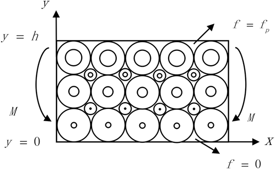
According to Zhang et al., the functionally graded SMA with gradient porosity was successfully fabricated in 2007 using a temporary space holder (NH4HCO3) and a conventional sintering method.Reference Zhang, Li and Zhang16 In this work, the whole material is regarded as a composite of the porous SMA and the dense SMA (which can be seen in Fig. 1). Assume that the porosities of the whole material along the “x” coordinate are constant, while the porosities of the whole material along the “y” coordinate are varying from the porosity f(y) = 0 at y = 0 (100% dense SMA) to f(y) = f p (100% porous SMA with porosity of f p) at y = h with a gradient function V(y), as
 $$f\left( y \right) = {f_{\rm{p}}}V\left( y \right)\quad ,$$
where f p is the porosity for the material at the layer y = h and V(y) is the gradient function of the porosity, which can be described by the following conditions,
 $$V\left( y \right) = \left\{ {\matrix{ 0 & {y = 0} \cr 1 & {y = h} \cr} } \right.\quad .$$
Mechanical model for porous SMA with gradient porosity under pure bending.

For different gradient functions, the distributions of the porosity are different. For simplicity, the following function of V(y) will be considered:
 $$V\left( y \right) = {\left( {{y \over h}} \right)^n}\quad ,$$
where “n” may be any real number; for different values of “n”, the gradient distribution is different.
According to the above assumption, the constitutive model for porous SMAs with gradient porosity under pure bending is then investigated; the image of the model for the system can be seen in Fig. 1. Based on the averaging method of the micromechanics, the average stress of each point for the whole material can be assumed as,
 $$\sigma \left( y \right) = \left[ {1 - V\left( y \right)} \right]{\sigma _{\rm{D}}} + V\left( y \right){\sigma _{\rm{P}}}\quad ,$$
where σD and σP are stress of the dense SMA phase and porous SMA phase, respectively.
According to Eshelby’s model with Mori–Tanaka mean field theory, the Young’s modulus of a porous SMA material E P is given by,
 $${{{E_{\rm{P}}}} \over {{E_{\rm{D}}}}} = {1 \over {1 + \eta {f_{\rm{p}}}}}\quad ,$$
where E D is the Young’s modulus of a dense SMA material, and for the spherical pores, η is given by,
 $$\eta = {{15} \over {7\left( {1 - {f_{\rm{p}}}} \right)}}\quad .$$
A. Thermo-elastic analysis of porous SMA with gradient porosity
For the thermo-elastic case, the average stress for the dense SMA and the porous SMA phases can be given by,
 $${\sigma _{\rm{D}}} = {E_{\rm{D}}}\varepsilon ;\;{\sigma _{\rm{P}}} = {E_{\rm{P}}}\varepsilon \quad ,$$
where ε is the axial strain of beam under pure bending, and according to the plane cross-section assumption, the axial strain of the beam can be expressed as,
 $$\varepsilon = {{y - {y_0}} \over \rho }\quad ,$$
where ρ is the curvature and the y 0 is the neutral axis, which can be derived on the basis that the resultant internal force and moment arising from the stress distribution through the thickness must balance any externally applied in-plane force or bending moment.
 $$\int_0^h {\sigma \left( y \right)b{\rm{d}}y = 0} \;{\rm{and}}\;{\rm{also}}\;\int_0^h {\sigma \left( y \right)yb{\rm{d}}y = M} \quad .$$
Substituting formulas (4), (7), and (8) in formula (9), we get,
 $$\int_0^h {\left[ {{E_{\rm{D}}} + V\left( y \right)\left( {{E_{\rm{P}}} - {E_{\rm{D}}}} \right)} \right]} {{y - {y_0}} \over \rho }b{\rm{d}}y = 0\quad ,$$
 $$\int_0^h {\left[ {{E_{\rm{D}}} + V\left( y \right)\left( {{E_{\rm{P}}} - {E_{\rm{D}}}} \right)} \right]} {{y - {y_0}} \over \rho }yb{\rm{d}}y = M\quad .$$
Then, the curvature ρ and the neutral axis y 0 can easily be obtained from (10) and (11),
 $$\rho = {{12E_{\rm{P}}^{\rm{2}} + {n^2}\left( {{n^2} + 4n + 7} \right)E_{\rm{D}}^2 + 4n\left( {{n^2} + 4n + 7} \right){E_{\rm{D}}}{E_{\rm{P}}}} \over {12\left( {n + 3} \right){{\left( {n + 2} \right)}^2}\left( {n{E_{\rm{D}}} + {E_{\rm{P}}}} \right)}}\quad ,$$
 $${y_0} = {{\left( {n + 1} \right)\left( {n{E_{\rm{D}}} + 2{E_{\rm{P}}}} \right)} \over {2\left( {n + 2} \right)\left( {n{E_{\rm{D}}} + {E_{\rm{P}}}} \right)}}h\quad .$$
The stress distribution can be obtained using the general expressions of (4), (7), (8), (12), and (13), and several particular cases of gradation can be treated just by assigning the appropriate value to parameter “n”.
 $$\sigma \left( y \right) = {1 \over \rho }\left( {{{{E_{\rm{P}}} - {E_{\rm{D}}}} \over {{h^n}}}{y^{n + 1}} - {{{E_{\rm{P}}} - {E_{\rm{D}}}} \over {{h^n}}}{y_0}{y^n} + {E_{\rm{D}}}y - {E_{\rm{D}}}{y_0}} \right)\quad .$$
B. Transformation analysis of porous SMA with gradient porosity
Assume that the whole material is initially in elastic austenite state; with the increasing loadings, the material may transform from austenite to martensite and then the martensite volume fraction ξ starts from zero and increases. The Young’s modulus of the material E i(ξ) (i = D represents the dense SMA; i = P represents the porous SMA) is also different for the different loading cases,
 $${E_{\rm{i}}}\left( \xi \right) = \left( {1 - \xi } \right){E_{{\rm{iA}}}} + \xi {E_{{\rm{iM}}}}\quad ,$$
where E iA and E iM are the Young’s moduli of austenite and martensite phase for dense SMA phase and porous SMA phase, respectively.
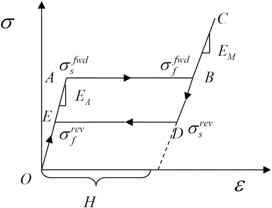
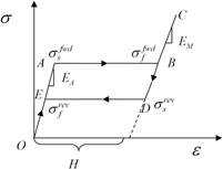
To get the analytical solution, an ideal elastoplastic constitutive model is selected to simulate the phase transformation of the SMAs. To illustrate the basic features of the FG-SMA material, the loading–unloading curve is schematized in Fig. 2. During loading, there are three states: elasticity (OA: complete austenite), transformation from austenitic to the martensitic phase (AB), and post-transformational elasticity (BC: complete martensite). The unloading responses include three states too, corresponding to CD, DE, and EO.
Stress–Strain relation of porous SMA with gradient porosity.

Let H denote the maximum transformation strain.  $\sigma _{\rm{s}}^{{\rm{fwd}}}$ be the initial phase transformation critical stress, and
 $\sigma _{\rm{s}}^{{\rm{rev}}}$ be the initial reverse phase transformation critical stress.
 $\sigma _{\rm{f}}^{{\rm{fwd}}}$ be the final phase transformation critical stress, and
 $\sigma _{\rm{f}}^{{\rm{rev}}}$ be the final reverse phase transformation critical stress. For the ideal elastoplastic constitutive model, assume that
 $\sigma _{\rm{s}}^{{\rm{fwd}}} = \sigma _{\rm{f}}^{{\rm{fwd}}},\;\sigma _{\rm{s}}^{{\rm{rev}}} = \sigma _{\rm{f}}^{{\rm{rev}}}$. According to Zhao et al.,Reference Zhao, Taya, Kang and Kawasaki24 for porous SMA, the initial and final martensitic transformation stresses
 $\sigma _{{\rm{Ms}}}^{\rm{P}}$ and
 $\sigma _{{\rm{Mf}}}^{\rm{P}}$ can be obtained by the relation
 $$\sigma _{{\rm{Ms}}}^{\rm{P}} = \left[ {1 - f\left( y \right)} \right]\sigma _{{\rm{Ms}}}^{\rm{D}}\;{\rm{and}}\;\sigma _{{\rm{Mf}}}^{\rm{P}} = \left[ {1 - f\left( y \right)} \right]\sigma _{{\rm{Mf}}}^{\rm{D}}\quad .$$
Considering the tensile compressive asymmetry of the SMAs, the initial and final martensitic transformation stresses  $\sigma _{{\rm{Ms}}}^{\rm{D}}$ and
 $\sigma _{{\rm{Mf}}}^{\rm{D}}$ can be obtained by
 $$\sigma _{{\rm{Ms}}}^{\rm{D}} = \left\{ \matrix{ \sigma _{{\rm{Mcs}}}^{\rm{D}}\quad {\rm{under}}\;{\rm{compression}} \hfill \cr \sigma _{{\rm{Mts}}}^{\rm{D}}\quad {\rm{under}}\;{\rm{tension}} \hfill \cr} \right.\quad .$$
Then, the Young’s modulus of the material in Eq. (15) can be degenerated to,
 $${E_{\rm{i}}} = \left\{ \matrix{ {E_{{\rm{iA}}}}\quad {\rm{when}}\;\xi = 0 \hfill \cr {E_{{\rm{iM}}}}\quad {\rm{when}}\;\xi \ne 0 \hfill \cr} \right.\quad .$$
The Mises’ yield criterion is chosen as the yield criterion of phase transformation; the effective stress can be described as
 $${\sigma _{\rm{e}}} = \sqrt {{3 \over 2}{{\sigma '}_{ij}}{{\sigma '}_{ij}}} \quad ,$$
where  ${\sigma '_{ij}} = {\sigma _{ij}} - {{{\sigma _{kk}}} / 3}$ is the deviatoric part of the stress σij. For the current pure bending problem of the system in this work, because there is only tension or compressive stress in the system, the problem can be degenerated to the one-dimensional case. According to (19), for one-dimensional case with the stress σij = [σ 0 0 0 0 0]T; the effective stress can be calculated by
 $${\sigma _{\rm{e}}} = \sigma \quad .$$
To get the analytical solution of the porous SMAs with gradient porosity after the transformation occurs, stress distributions should be performed to demonstrate the phase transformation. As a starting point, the initial phase transition point should be determined first. To accomplish this task, the effective stress of the system is calculated first, and the stress distributions can be obtained by (14) for different values of n. Then, for different n, the maximum tension value and the maximum compression value of the effective stresses can easily be obtained.
Based on the following numerical work, the effective stresses will show a maximum tension value in the upper bound (at y = h, 100% porous SMA with porosity of f p) and a maximum compression value in the lower bound (at y = 0 with 100% dense SMA). When the maximum value of the effective stress at y = h in the 100% porous SMA layer is equal to the yield stress of the porous SMA, the system begins the transformation process; then, the system will not be elastic and the stress distribution will be changed. So both the effective stresses of the porous SMA phase and the dense SMA phase should be used to judge whether the system is transformed or not, and the critical load M cr1 can be calculated by the boundary condition  ${\left. {{\sigma _{\rm{e}}} = \sigma _{{\rm{Ms}}}^{\rm{P}}} \right|_{y = h}}$. After the transformation occurs, the stress distribution will be analyzed next.
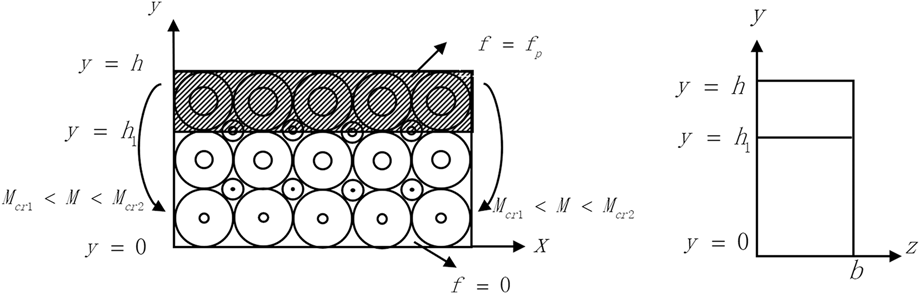
With the increasing loading M > M cr1, the upper layer is transformed first and expand downward, as shown in Fig. 3. For the part from h 1 to h, the phase transformation occurs, and according to (18), the Young’s modulus is changed to E iM, and for the part from 0 to h 1, no phase transformation occurs and the Young’s modulus is still E iA. To get the analytical solution, the case with n = 1 is chosen in this work to deduce the following stress distributions for the case when the transformation occurs. Then, based on the averaging method of the micromechanics (4), the average stress for the whole material can be expressed as
 $$\sigma \left( y \right) = \left\{ {\matrix{ {\left[ {{E_{{\rm{DA}}}} + {y \over h}\left( {{E_{{\rm{PA}}}} - {E_{{\rm{DA}}}}} \right)} \right]{{y - {y_1}} \over {{\rho _1}}}\quad 0 \lt y \le {h_1}{\rm{\ }}} \cr {\left[ {{E_{{\rm{DM}}}} + {y \over h}\left( {{E_{{\rm{PM}}}} - {E_{{\rm{DM}}}}} \right)} \right]{{y - {y_1}} \over {{\rho _1}}}\quad {h_1} \lt y \le h{\rm{\ }}} \cr} } \right.\quad ,$$
where the curvature ρ1 and the neutral axis y 1 can also be derived on the basis that the resultant internal force and moment arising from the stress distribution through the thickness must balance any externally applied in-plane force or bending moment:
 $$\int_0^{{h_1}} {\sigma \left( y \right)b{\rm{d}}y + } \int_{{h_1}}^h {\sigma \left( y \right)b{\rm{d}}y = 0} \;{\rm{and}}\;{\rm{also}}\;\int_0^{{h_1}} {\sigma \left( y \right)yb{\rm{d}}y + \int_{{h_1}}^h {\sigma \left( y \right)yb{\rm{d}}y} = M\quad .}$$
Mechanical model with M cr2 > M > M cr1.

Substituting formula (21) in formula (22), we get,
 $$\int_0^{{h_1}} {\left[ {{E_{{\rm{DA}}}} + {y \over h}\left( {{E_{{\rm{PA}}}} - {E_{{\rm{DA}}}}} \right)} \right]} {{y - {y_1}} \over {{\rho _1}}}b{\rm{d}}y + \int_{{h_1}}^h {\left[ {{E_{{\rm{DM}}}} + {y \over h}\left( {{E_{{\rm{PM}}}} - {E_{{\rm{DM}}}}} \right)} \right]} {{y - {y_1}} \over {{\rho _1}}}b{\rm{d}}y = 0\quad ,$$
 $$\int_0^{{h_1}} {\left[ {{E_{{\rm{DA}}}} + {y \over h}\left( {{E_{{\rm{PA}}}} - {E_{{\rm{DA}}}}} \right)} \right]} {{y - {y_1}} \over {{\rho _1}}}yb{\rm{d}}y + \int_{{h_1}}^h {\left[ {{E_{{\rm{DM}}}} + {y \over h}\left( {{E_{{\rm{PM}}}} - {E_{{\rm{DM}}}}} \right)} \right]} {{y - {y_1}} \over {{\rho _1}}}yb{\rm{d}}y = M\quad .$$
Then, the curvature ρ and the neutral axis y 0 can easily be obtained from (23) and (24),
 $${y_1} = {{{E_{{\rm{DM}}}}\left( {{h^3} - 3h_1^2h + 2h_1^3} \right) + {E_{{\rm{PM}}}}\left( {2{h^3} - 2h_1^3} \right) + {E_{{\rm{DA}}}}\left( {3h_1^2h - 2h_1^3} \right) + {E_{{\rm{PA}}}}2h_1^3} \over {3\left[ {{E_{{\rm{DM}}}}\left( {{h^2} - 2{h_1}h + h_1^2} \right) + {E_{{\rm{PM}}}}\left( {{h^2} - h_1^2} \right) + {E_{{\rm{DA}}}}\left( {2{h_1}h - h_1^2} \right) + {E_{{\rm{PA}}}}h_1^2} \right]}}\quad ,$$
 $${\rho _1} = \left[ {A{E_{{\rm{DM}}}} + B{E_{{\rm{PM}}}} + C{E_{{\rm{DA}}}} + D{E_{{\rm{PA}}}}} \right]{b \over M}\quad ,$$
where  $A = {{{h^3}} \over {12}} - {{h_1^3} \over 3} - {{{h^2}{y_0}} \over 6} + {{h_1^2{y_0}} \over 2} - {{h_1^3{y_0}} \over {3h}} + {{h_1^4} \over {4h}}$,
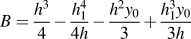 $B = {{{h^3}} \over 4} - {{h_1^4} \over {4h}} - {{{h^2}{y_0}} \over 3} + {{h_1^3{y_0}} \over {3h}}$,
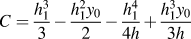 $C = {{h_1^3} \over 3} - {{h_1^2{y_0}} \over 2} - {{h_1^4} \over {4h}} + {{h_1^3{y_0}} \over {3h}}$, and
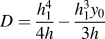 $D = {{h_1^4} \over {4h}} - {{h_1^3{y_0}} \over {3h}}$.
For any value of loading M cr2 > M > M cr1, the h 1 can be calculated by the boundary condition  ${\left. {{\sigma _{\rm{e}}} = \sigma _{{\rm{Ms}}}^{\rm{P}}} \right|_{y = {h_1}}}$. Till the phase transformation happens at the lower layer, finish this phase. And the critical load M cr2 can be calculated by the boundary condition
 ${\left. {{\sigma _{\rm{e}}} = \sigma _{{\rm{Ms}}}^{\rm{P}}} \right|_{y = 0}}$.
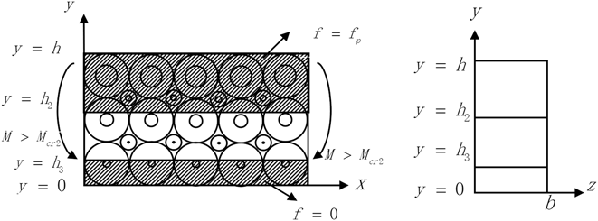
With the increasing loading M > M cr2, the lower layer begins the transformation and runs up to h 2 and the upper layers continue to transform and runs up to h 3, which can be seen in Fig. 4; for the part from h 3 to h and the part from 0 to h 2, the phase transformation occurs and according to (18), the Young’s moduli are changed to E iM, and for the part from h 2 to h 3, no phase transformation occurs and the Young’s moduli are still E i. Then, based on the averaging method of the micromechanics (4), the average stress for the whole material can be expressed as
 $$\sigma \left( y \right) = \left\{ {\matrix{ {\left[ {{E_{{\rm{DM}}}} + {y \over h}\left( {{E_{{\rm{PM}}}} - {E_{{\rm{DM}}}}} \right)} \right]{{y - {y_2}} \over {{\rho _2}}}\quad 0 \lt y \le {h_2}} \cr {\left[ {{E_{{\rm{DA}}}} + {y \over h}\left( {{E_{{\rm{PA}}}} - {E_{{\rm{DA}}}}} \right)} \right]{{y - {y_2}} \over {{\rho _2}}}\quad {h_2} \lt y \le {h_3}} \cr {\left[ {{E_{{\rm{DM}}}} + {y \over h}\left( {{E_{{\rm{PM}}}} - {E_{{\rm{DM}}}}} \right)} \right]{{y - {y_2}} \over {{\rho _2}}}\quad {h_3} \lt y \le h} \cr} } \right.\quad ,$$
where the curvature ρ2 and the neutral axis y 2 can also be derived on the basis that the resultant internal force and moment arising from the stress distribution through the thickness must balance any externally applied in-plane force or bending moment:
 $$\int_0^{{h_2}} {\sigma \left( y \right)b{\rm{d}}y + } \int_{{h_2}}^{{h_1}} {\sigma \left( y \right)b{\rm{d}}y} + \int_{{h_1}}^h {\sigma \left( y \right)b{\rm{d}}y} = 0\;{\rm{and}}\;\int_0^{{h_2}} {\sigma \left( y \right)yb{\rm{d}}y + } \int_{{h_2}}^{{h_1}} {\sigma \left( y \right)yb{\rm{d}}y} + \int_{{h_1}}^h {\sigma \left( y \right)yb{\rm{d}}y} = M\quad .$$
Mechanical model with M > M cr2.

Substituting formula (27) in formula (28), we get,
 $$\int_0^{{h_2}} {\left[ {{E_{{\rm{DM}}}} + {y \over h}\left( {{E_{{\rm{PM}}}} - {E_{{\rm{DM}}}}} \right)} \right]} {{y - {y_2}} \over {{\rho _2}}}b{\rm{d}}y + \int_{{h_2}}^{{h_3}} {\left[ {{E_{{\rm{DA}}}} + {y \over h}\left( {{E_{{\rm{PA}}}} - {E_{{\rm{DA}}}}} \right)} \right]} {{y - {y_2}} \over {{\rho _2}}}b{\rm{d}}y + \int_{{h_3}}^h {\left[ {{E_{{\rm{DM}}}} + {y \over h}\left( {{E_{{\rm{PM}}}} - {E_{{\rm{DM}}}}} \right)} \right]} {{y - {y_2}} \over {{\rho _2}}}b{\rm{d}}y = 0\quad ,$$
 $$\int_0^{{h_2}} {\left[ {{E_{{\rm{DM}}}} + {y \over h}\left( {{E_{{\rm{PM}}}} - {E_{{\rm{DM}}}}} \right)} \right]} {{y - {y_2}} \over {{\rho _2}}}yb{\rm{d}}y + \int_{{h_2}}^{{h_3}} {\left[ {{E_{{\rm{DA}}}} + {y \over h}\left( {{E_{{\rm{PA}}}} - {E_{{\rm{DA}}}}} \right)} \right]} {{y - {y_2}} \over {{\rho _2}}}yb{\rm{d}}y + \int_{{h_3}}^h {\left[ {{E_{{\rm{DM}}}} + {y \over h}\left( {{E_{{\rm{PM}}}} - {E_{{\rm{DM}}}}} \right)} \right]} {{y - {y_2}} \over {{\rho _2}}}yb{\rm{d}}y = 0\quad .$$
Then, the curvature ρ and the neutral axis y 0 can easily be obtained by (29) and (30):
 $${y_2} = {{{E_{{\rm{DM}}}}\left( {3h_2^2h - 2h_2^3 + {h^3} - 3h_3^2h + 2h_3^3} \right) + {E_{{\rm{PM}}}}\left( {2h_2^3 + 2{h^3} - 2h_3^3} \right) + {E_{{\rm{DA}}}}\left( {3h_3^2h - 3h_2^2h - 2h_3^3 + 2h_2^3} \right) + {E_{{\rm{PA}}}}\left( {2h_3^3 - 2h_2^3} \right)} \over {3\left[ {{E_{{\rm{DM}}}}\left( {2{h_2}h - h_2^2 + {h^2} - 2{h_3}h + h_3^2} \right) + {E_{{\rm{PM}}}}\left( {{h^2} + {h^2} - h_3^2} \right) + {E_{{\rm{DA}}}}\left( {2{h_3}h - 2{h_2}h - h_3^2 + h_2^2} \right) + {E_{{\rm{PA}}}}\left( {h_3^2 - h_2^2} \right)} \right]}}\quad ,$$
 $${\rho _2} = \left[ {H{E_{{\rm{DM}}}} + I{E_{{\rm{PM}}}} + J{E_{{\rm{DA}}}} + K{E_{{\rm{PA}}}}} \right]{b \over M}\quad ,$$
where  $H = {{h_2^3} \over 3} - {{h_3^3} \over 3} + {{h_3^2{y_0}} \over 2} - {{h_2^2{y_0}} \over 2} + {{h_3^4} \over {4h}} - {{h_2^4} \over {4h}} - {{h_3^3{y_0}} \over {3h}} + {{h_2^3{y_0}} \over {3h}} + {{{h^3}} \over {12}} - {{{h^2}{y_0}} \over 6}$,
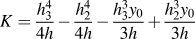 $K = {{h_{\rm{3}}^4} \over {4h}} - {{h_2^4} \over {4h}} - {{h_{\rm{3}}^3{y_0}} \over {3h}} + {{h_2^3{y_0}} \over {3h}}$,
 $I = {{h_2^4} \over {4h}} - {{h_{\rm{3}}^4} \over {4h}} + {{h_{\rm{3}}^3{y_0}} \over {3h}} - {{h_2^3{y_0}} \over {3h}} + {{{h^3}} \over 4} - {{{h^2}{y_0}} \over 3}$,
 $J = {{h_1^3} \over 3} - {{h_2^3} \over 3} - {{h_{\rm{3}}^2{y_0}} \over 2} + {{h_2^2{y_0}} \over 2} - {{h_{\rm{3}}^4} \over {4h}} + {{h_2^4} \over {4h}} + {{h_{\rm{3}}^3{y_0}} \over {3h}} - {{h_2^3{y_0}} \over {3h}}$.
For any value of the loading M > M cr2, the h 3 and h 2 can be calculated by the boundary condition  ${\left. {{\sigma _{\rm{e}}} = \sigma _{{\rm{Ms}}}^{\rm{P}}} \right|_{y = {h_3}}}$ and
 ${\left. {{\sigma _{\rm{e}}} = \sigma _{{\rm{Ms}}}^{\rm{P}}} \right|_{y = {h_2}}}$. Loading is continued till all the material is transformed to martensite.
III. NUMERICAL RESULTS
The above developed theory can be applied in modeling the macro-mechanical properties for porous SMAs with gradient porosity. The material parameters for dense SMA in Table I are chosen to be used during in the numerical calculation for modeling the behaviors of the porous SMAs.
Parameters used in the calculation for the thermo-elastic system.Reference Zhao, Taya, Kang and Kawasaki24,Reference Entchev and Lagoudas25

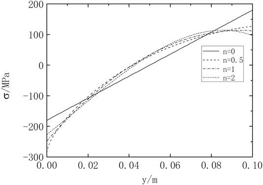
Figure 5 shows the distributions of the effective stress through the system with different n. The dotted curve represents the distribution of the average stress with n = 2, the solid curve corresponds to the distribution of the effective stress with n = 0, the dash curve represents the distribution of the average stress with n = 0.5, and the dash–dot curve represents the distribution of the average stress with n = 1. As seen in Fig. 5, the stresses distribution through the whole material depends on the different values of n, while for different n, the effective stresses show a maximum tension value at the upper bound (100% porous SMA with porosity of f p) and a maximum compression value at the lower bound (100% dense SMA). For the case n = 1 which can be seen in the dash–dot curve on Fig. 5, the effective stresses show a maximum tension value at the upper bound (at h = 0.1, 100% porous SMA with porosity of f p) and a maximum compression value at the lower bound (at h = 0 with 100% dense SMA). When the maximum value of the effective stress at h = 0.1 in the 100% porous SMA layer is equal to the yield stress of the porous SMA, the system begins the transformation and the system will not be elastic and the stress distribution will be changed.
Stress distributions through the whole system with different n for M = 15 MPa.

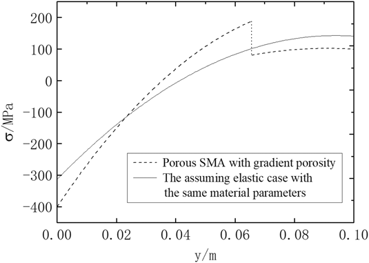
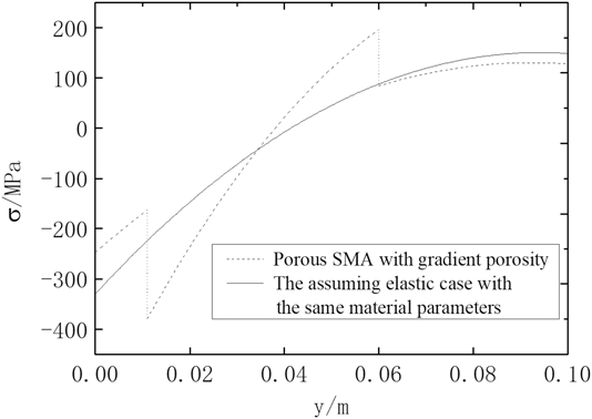
Figure 6 shows the distributions of the effective stress through the system with n = 1 for M = 18.93 MPa. The dotted curve represents the distribution of the average stress when the transformation occurs, and the solid curve corresponds to the distributions of the effective stress for the assumed pure elastic case with the same material parameters. As seen in Fig. 6, after the phase transformation occurs, the maximum effective stresses for the compression part and the tension part decrease. The curve in Fig. 6 is discontinuous for the ideal elastoplastic model used in this work. The effective stress distributions through the whole system with n = 1 for M = 19.93 MPa can be seen Fig. 7, where the dotted curve represents the distribution of the average stress at the parts when the transformation occurs and the solid curve corresponds to the distributions of the effective stress of the assumed pure elastic case with the same material parameters. As seen in Fig. 7, after the phase transformation, the effective stresses for the compression part and the tension part decrease.
Stress distributions through the whole system with n = 1 for M = 18.93 MPa.

Stress distributions through the whole system with n = 1 for M = 19.93 MPa.

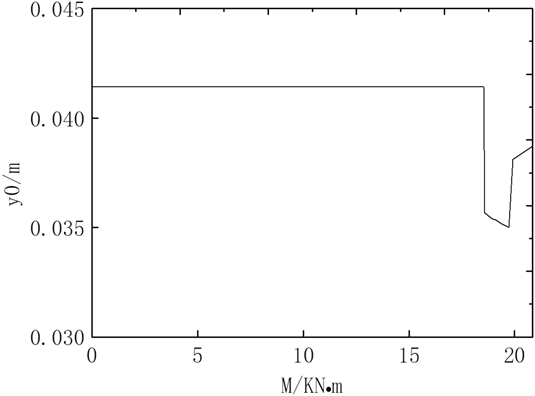
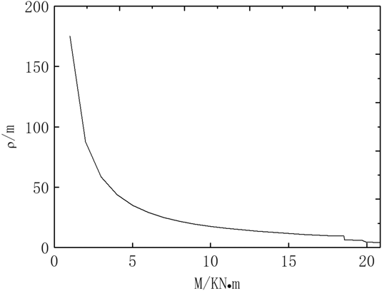
Figure 8 shows the neutral axis distribution of the system with the increasing M. It can be shown that, for the elastic phase, the neutral axis for the system show a constant value, and the neutral axis show a big mutation when the transformation happens in the upper layer and in the lower layer for the ideal elastoplastic model. With the increasing bending load, the position of the neutral axis is still in the system, which means that there is always a zero stress point in the system. With the increasing loading M, the phase transformation will infinitely be close to the perfect phase transformation and it is hard to get to a complete phase transition. Figure 9 shows the radius of the curvature distribution of the system with the increasing M, and it can be seen from Fig. 9 that with the increasing M the radius of the curvature will infinitely be close to zero and also show a big mutation when the transformation occurs in the upper layer and in the lower layer for the ideal elastoplastic model.
Neutral axis distribution of the system with increasing M.

Radius of the distribution through the whole system with increasing M.

IV. CONCLUSIONS
A constitutive model for porous SMAs with gradient porosity by micromechanical average theory is given in this work. The whole material is regarded as a gradient composite of the porous SMA and the dense SMA, in which the component fractions of the porous SMA show gradient changes over geometric dimensions. Numerical result shows that after the phase transformation, the effective stresses of the material decrease for the compression part and the tension part. And with the increasing loading M, the phase transformation will infinitely be close to the perfect phase transformation, but it is hard to get to a complete phase transition.
ACKNOWLEDGMENTS
The authors acknowledge the financial support of National Natural Science Foundation of China (Nos. 11502284, 51505483, 11802206, and 51608522), and it is also supported by the Fundamental Research Funds for the Central Universities of China (3122015C019).