1 Introduction
Dense non-Brownian suspensions are complex non-Newtonian fluids made of particles (of hydraulic diameter:
 $d_{p}=2a>1~\unicode[STIX]{x03BC}\text{m}$
) that are immersed in a viscous fluid where Brownian motion is neglected (
 $Pe=(6\unicode[STIX]{x03C0}\unicode[STIX]{x1D702}_{f}(d_{p}/2)^{3}\dot{\unicode[STIX]{x1D6FE}})/\unicode[STIX]{x1D70C}_{f}\unicode[STIX]{x1D705}T\gg 1$
;
 $Re_{p}=(\dot{\unicode[STIX]{x1D6FE}}(d_{p}/2)^{2})/\unicode[STIX]{x1D702}_{f}\ll 1$
). Here,
 $\dot{\unicode[STIX]{x1D6FE}}=\sqrt{2\unicode[STIX]{x1D640}\boldsymbol{ :}\unicode[STIX]{x1D640}}$
is the shear rate and
 $\unicode[STIX]{x1D640}$
is the local rate of strain tensor such that
 $\unicode[STIX]{x1D640}=0.5(\unicode[STIX]{x1D735}\boldsymbol{U}+\unicode[STIX]{x1D735}\boldsymbol{U}^{\text{T}})$
;
 $\unicode[STIX]{x1D70C}_{f}$
is the fluid phase density,
 $\unicode[STIX]{x1D702}_{f}$
the fluid phase kinematic viscosity,
 $\unicode[STIX]{x1D6FC}_{f}$
the fluid phase thermal diffusivity,
 $T$
temperature and
 $\unicode[STIX]{x1D705}$
is the Boltzmann constant. Suspension flows are present in many applications at different scales as in chemical, process, civil, mechanical, geological, biological and industrial engineering (e.g. cosmetics, detergents, rivers, drilling muds, blood, concrete, oil and fuels, food processing, etc.). Thus, understanding the flow behaviour of these complex flows is essential for improving and predicting optimal future designs of systems where dense suspensions may be present (Guazzelli & Morris Reference Guazzelli and Morris2011; Guazzelli Reference Guazzelli2017). Throughout this manuscript the word ‘suspension flow’ will be employed to describe bulk laminar flow that is made of ‘spherical rigid monodisperse particles that are immersed in a Newtonian viscous fluid’.
1.1 Shear-induced particle migration in suspension flows
Particle transport in suspension flows has been widely studied in the literature. When a non-Brownian (or non-colloidal) suspension is in flow, the phenomenon of shear-induced particles migration (SIM) may occur as a self-diffusion phenomenon depending on inertial forces, viscous forces, flow type, geometry, etc. and on the suspension properties (effective viscosity, particles roughness, particles interactions frequency, polydispersity, etc.). Suspension flows are known to exhibit a non-Newtonian behaviour manifested by the presence of two normal-stress differences,
 $N_{1}$
and
 $N_{2}$
, and the SIM. In dense suspensions flows of rigid spheres the normal-stress differences are measured and known to be linearly proportional to the shear rate
 $(\dot{\unicode[STIX]{x1D6FE}})$
(Dbouk Reference Dbouk2011; Dbouk, Lobry & Lemaire Reference Dbouk, Lobry and Lemaire2013a
) and to vary as a function of the volume fraction of particles
 $\unicode[STIX]{x1D719}$
. The SIM phenomenon can be seen as an equilibrium state transition from a homogeneous distribution of particles toward an inhomogeneous one where the volume fraction of particles (
 $\unicode[STIX]{x1D719}=V_{particles}/V_{total}$
) changes locally during the flow. This inhomogeneous distribution of particles is usually not favoured for many industrial processes where final products of a homogeneous nature are required. For such reasons, researchers have made huge efforts trying to quantify and predict the SIM in different geometries. For example, experiments on concentrated suspension flow in a Couette cell revealed that the SIM occurs from the inner to the outer cylinder, while in the parallel-plate geometry, no SIM is observed (Chapman Reference Chapman1990; Chow et al.
Reference Chow, Sinton, Iwamiya and Stephens1994; Merhi et al.
Reference Merhi, Lemaire, Bossis and Moukalled2005; Bricker & Butler Reference Bricker and Butler2006; Kim, Lee & Kim Reference Kim, Lee and Kim2008). In pressure-driven flows in channels, the SIM occurs from the wall to the centreline (Lyon & Leal Reference Lyon and Leal1998; Miller & Morris Reference Miller and Morris2006; Semwogerere, Morris & Weeks Reference Semwogerere, Morris and Weeks2007). Many authors have investigated the SIM in different geometries (Gadala-Maria & Acrivos Reference Gadala-Maria and Acrivos1980; Leighton & Acrivos Reference Leighton and Acrivos1987a
,Reference Leighton and Acrivos
b
; Lhuillier Reference Lhuillier2009; Dbouk Reference Dbouk2011). In recent efforts, the suspension rheology and granular material rheology were unified where the nature of the suspension dynamics is a result of both frictional and hydrodynamic forces (see Boyer, Guazzelli & Pouliquen Reference Boyer, Guazzelli and Pouliquen2011a
; Boyer, Pouliquen & Guazzelli Reference Boyer, Pouliquen and Guazzelli2011b
; Andreotti, Forterre & Pouliquen Reference Andreotti, Forterre and Pouliquen2013).
1.2 Heat transfer in suspension flows
In contrast with the amount of research work done in the field of particle transport in suspension flows, conjugate heat transfer in suspension flows has been rarely investigated either experimentally or numerically.
Experimentally speaking, Metzger, Rahli & Yin (Reference Metzger, Rahli and Yin2013) were the only researchers, to our knowledge, who recently revealed the topic of conjugate heat transfer in dense suspension flows of rigid spheres after the past works of Shin & Lee (Reference Shin and Lee2000) and the rare older efforts by Ahuja (Reference Ahuja1975a
,Reference Ahuja
b
), Sohn & Chen (Reference Sohn and Chen1981) three decades ago. Ahuja (Reference Ahuja1975a
,Reference Ahuja
b
) demonstrated that heat transfer is significantly augmented in sheared suspensions of polystyrene particles. From experimental data, they proposed a suspension effective thermal conductivity constitutive equation as a function of the particle rotation
 $\unicode[STIX]{x1D714}$
, the shear rate
 $\dot{\unicode[STIX]{x1D6FE}}$
, the thermal Péclet number
 $(Pe_{d_{p}}=\dot{\unicode[STIX]{x1D6FE}}d_{p}^{2}/\unicode[STIX]{x1D6FC}_{f})$
and the volume fraction of particles
 $\unicode[STIX]{x1D719}$
. Sohn & Chen (Reference Sohn and Chen1981) measured experimentally the suspension effective thermal conductivity
 $k_{S}$
for suspensions of rigid non-colloidal beads (2.9 and 0.3 mm in diameter) at two volume fractions (
 $\unicode[STIX]{x1D719}=0.15$
and 0.30). They observed in a Couette flow experiment that
 $k_{S}$
displays a power-law relationship with
 $Pe_{d_{p}}$
such that
 $k_{S}\propto Pe_{d_{p}}^{1/2}$
for
 $(300<Pe_{d_{p}}<2000)$
. Shin & Lee (Reference Shin and Lee2000) measured also
 $k_{S}$
in a Couette cell that is sheared by the outer cylinder at different shear rate values and for four different particle diameters
 $d_{p}=25$
, 100, 180,
 $300~\unicode[STIX]{x03BC}\text{m}$
. Shin & Lee (Reference Shin and Lee2000) found
 $k_{S}$
to increase with shear rate and particle size, with an unexplained saturation at large shear rates
 $(\dot{\unicode[STIX]{x1D6FE}}>300~\text{s}^{-1})$
. Recently, Metzger et al. (Reference Metzger, Rahli and Yin2013) conducted thermal measurements on an isodense concentrated suspension sheared by the inner cylinder in a concentric cylindrical Couette cell. They showed the role of the shear-induced diffusion in enhancing overall heat transfer in isodense concentrated suspension flows. They measured with good precision (
 $\pm 0.02\,^{\circ }\text{C}$
) the temperature decay of the inner cylinder at a bulk volume fraction of 35 % of PMMA (polymethyl methacrylate) in rigid spheres 2 and 1 mm in diameter. Using the same densities and same thermal properties for the particles and the surrounding fluid, Metzger et al. (Reference Metzger, Rahli and Yin2013) showed that the temperature decay rate is affected by: the SIM, the applied shear-rate value and the
 $Pe_{d_{p}}$
number. They observed that the SIM occurs from the inner to the outer cylinder in the Couette cell, as is well known for this geometry.
Numerically speaking, Wu et al. (Reference Wu, Zhou, Aubry, Antaki and Massoudi2017) were among the first researchers to our knowledge who presented a macroscopic modelling approach for suspension flows including heat transfer. However, in Wu et al. (Reference Wu, Zhou, Aubry, Antaki and Massoudi2017) the modelling was not complete. They did not take into account the influence of the shear rate, volume fraction and
 $Pe_{d_{p}}$
number on the suspension effective thermal properties as observed experimentally by Metzger et al. (Reference Metzger, Rahli and Yin2013). Moreover, Wu et al. (Reference Wu, Zhou, Aubry, Antaki and Massoudi2017) modelled the suspension viscosity only as a function of the volume fraction
 $\unicode[STIX]{x1D719}$
. However, a suspension viscosity modelled as shear rate independent can be valid only for particles that are small compared to a critical value of diameter (i.e.
 $d_{p}\geqslant 10~\unicode[STIX]{x03BC}\text{m}$
). Recently, Rebouas et al. (Reference Rebouas, Siqueira, de Souza Mendes and Carvalho2016) showed that for small particles (
 $d_{p}\geqslant 1~\unicode[STIX]{x03BC}\text{m}$
) the suspension effective viscosity
 $\unicode[STIX]{x1D702}_{S}$
becomes very sensitive to both the shear rate
 $\dot{\unicode[STIX]{x1D6FE}}$
and the volume fraction
 $\unicode[STIX]{x1D719}$
of particles and thus would be better represented by both
 $\dot{\unicode[STIX]{x1D6FE}}$
and
 $\unicode[STIX]{x1D719}$
-dependent constitutive models
 $(\unicode[STIX]{x1D702}_{S}=\unicode[STIX]{x1D702}_{S}(\dot{\unicode[STIX]{x1D6FE}},\unicode[STIX]{x1D719}))$
.
2 Constitutive modelling of heat transfer and shear-induced migration in suspension flows
In this contribution, constitutive modelling and simulation are developed, generalized and validated for both heat transfer and shear-induced particle migration in dense non-colloidal suspension flows (monodispersed rigid spheres that are in thermal equilibrium and suspended in a Newtonian viscous fluid). The present developments are based on coupling past theory and measurements for the effective thermal conductivity in porous materials at zero shear rate (Sugawara & Yoshizawa Reference Sugawara and Yoshizawa1961, Reference Sugawara and Yoshizawa1962; Ahuja Reference Ahuja1975a
,Reference Ahuja
b
; Sohn & Chen Reference Sohn and Chen1981) with more recent effective thermal diffusivity measurements of sheared suspensions (Shin & Lee Reference Shin and Lee2000; Metzger et al.
Reference Metzger, Rahli and Yin2013). The suspension effective heat transfer affected by the shear rate, the phenomenon of shear-induced particle migration (SIM) (presented by the suspension balance model (SBM) of Nott & Brady Reference Nott and Brady1994; Morris & Brady Reference Morris and Brady1998; Morris & Boulay Reference Morris and Boulay1999), the buoyancy effects and the thermal Péclet number (
 $Pe_{d_{p}}=\dot{\unicode[STIX]{x1D6FE}}d_{p}^{2}/\unicode[STIX]{x1D6FC}_{f}$
) at the particle scale are all considered in the present modelling. A novel three-dimensional (3-D) computational fluid dynamics (CFD) macroscopic model is developed and constructed in the open source CFD toolbox (OpenFOAM 2017) based on the numerical finite volume method (FVM) (Moukalled, Mangani & Darwish Reference Moukalled, Mangani and Darwish2015). The constructed 3-D CFD model is implemented in OpenFOAM (2017) as a new solver and based on the PIMPLE algorithm (Moukalled et al.
Reference Moukalled, Mangani and Darwish2015) which allows dynamic adaptive time step handling for faster and more stable computations over the iterations. The influence of the temperature, the shear rate and the particle volume fraction on the suspension effective viscosity, on the suspension effective thermal properties and on the fluid density are all taken into account (assuming a slightly compressible temperature-dependent viscous fluid with radiative heat transfer neglected and where the fluid is in thermal equilibrium with the particles).
2.1 Shear-induced particle migration modelling
Numerical modelling and simulation of the SIM phenomena in suspension flows have been widely studied in the literature via different numerical approaches (Eulerian (Dbouk et al.
Reference Dbouk, Lobry, Lemaire and Moukalled2013b
), Lagrangian (Gallier et al.
Reference Gallier, Lemaire, Lobry and Peters2016; Peters et al.
Reference Peters, Ghigliotti, Gallier, Blanc, Lemaire and Lobry2016) and/or Eulerian–Lagrangian (Dbouk Reference Dbouk2016)). There are generally two continuum macroscopic models from the literature that have been applied to predict the SIM in dense suspension flows: the diffusive flux model developed by Phillips et al. (Reference Phillips, Armstrong, Brown, Graham and Abbott1992) and adopted by Merhi et al. (Reference Merhi, Lemaire, Bossis and Moukalled2005), Wu et al. (Reference Wu, Zhou, Aubry, Antaki and Massoudi2017) and the suspension balance model (SBM) of Nott & Brady (Reference Nott and Brady1994), Morris & Brady (Reference Morris and Brady1998), Morris & Boulay (Reference Morris and Boulay1999). The diffusive flux model by Phillips et al. (Reference Phillips, Armstrong, Brown, Graham and Abbott1992) has some drawbacks such as the presence of several numerical parameters to fit, in addition to the fact that it produces SIM even in the parallel-plate geometry which is usually not observed experimentally by Chapman (Reference Chapman1990), Chow et al. (Reference Chow, Sinton, Iwamiya and Stephens1994), Merhi et al. (Reference Merhi, Lemaire, Bossis and Moukalled2005). The SBM is considered in the present work to counter for the shear-induced particles migration modelling modified to account for the presence of slightly bulk inertia of the suspension flow. The SBM represents the migration flux of particles
 $\boldsymbol{J}_{s}$
as being proportional to the divergence of the particles stress second-rank tensor
 $\unicode[STIX]{x1D72E}_{p}$
such as
 $(\boldsymbol{J}_{s}\propto \unicode[STIX]{x1D735}\boldsymbol{\cdot }\unicode[STIX]{x1D72E}_{p})$
. The
 $\unicode[STIX]{x1D72E}_{p}$
can be obtained from normal-stress differences measurements and their dependence on the local shear rate
 $\dot{\unicode[STIX]{x1D6FE}}$
and the volume fraction of particles
 $\unicode[STIX]{x1D719}$
. The suspension effective kinematic viscosity
 $\unicode[STIX]{x1D702}_{S}$
can be obtained via rheometry measurements to constitute its law behaviour as a function of
 $\unicode[STIX]{x1D719}$
such that
 $\unicode[STIX]{x1D702}_{S}=f(\unicode[STIX]{x1D702}_{f},\unicode[STIX]{x1D719})$
(see Krieger & Dougherty Reference Krieger and Dougherty1959; Dbouk et al.
Reference Dbouk, Lobry and Lemaire2013a
) where
 $\unicode[STIX]{x1D702}_{f}$
represents the viscous fluid kinematic viscosity. The SBM has been validated previously in the literature and has well predicted the SIM in different geometries of dense suspension flows (i.e. pressure-driven flows in channels (Miller & Morris Reference Miller and Morris2006), Couette cell flows (Dbouk et al.
Reference Dbouk, Lobry, Lemaire and Moukalled2013b
)). Considering buoyancy effects and assuming hydrodynamic interactions in slightly compressible viscous suspension in a laminar flow, the main constitutive equations based on the SBM (continuity, momentum and mass conservation equations, respectively) can be written as the following:
 $$\begin{eqnarray}\displaystyle & \displaystyle \frac{\unicode[STIX]{x2202}\unicode[STIX]{x1D70C}}{\unicode[STIX]{x2202}t}+\unicode[STIX]{x1D735}\boldsymbol{\cdot }(\unicode[STIX]{x1D70C}\boldsymbol{U})=0, & \displaystyle\end{eqnarray}$$
 $$\begin{eqnarray}\displaystyle & \displaystyle \frac{\text{D}}{\text{D}t}(\unicode[STIX]{x1D70C}\boldsymbol{U})-\unicode[STIX]{x1D735}\boldsymbol{\cdot }\unicode[STIX]{x1D72E}+\unicode[STIX]{x0394}\unicode[STIX]{x1D70C}\boldsymbol{g}\unicode[STIX]{x1D719}=0, & \displaystyle\end{eqnarray}$$
 $$\begin{eqnarray}\displaystyle & \displaystyle \frac{\text{D}}{\text{D}t}(\unicode[STIX]{x1D719})=-\unicode[STIX]{x1D735}\boldsymbol{\cdot }\boldsymbol{J}_{\boldsymbol{t}}. & \displaystyle\end{eqnarray}$$
The material derivative operator
 $(\text{D}/\text{D}t)(\ast )$
acting on a
 $(\ast )$
quantity is defined as the following:
 $$\begin{eqnarray}\frac{\text{D}}{\text{D}t}(\ast )=\frac{\unicode[STIX]{x2202}(\ast )}{\unicode[STIX]{x2202}t}+(\boldsymbol{U}\boldsymbol{\cdot }\unicode[STIX]{x1D735})(\ast ),\end{eqnarray}$$
where
 $t$
denotes the time,
 $\unicode[STIX]{x0394}\unicode[STIX]{x1D70C}=(\unicode[STIX]{x1D70C}_{p}-\unicode[STIX]{x1D70C}_{f})$
,
 $\boldsymbol{U}$
is the averaged suspension velocity,
 $\unicode[STIX]{x1D719}$
the volume fraction of particles and the suspension overall stress tensor
 $\unicode[STIX]{x1D72E}$
is defined as
 $(\unicode[STIX]{x1D72E}=\unicode[STIX]{x1D72E}_{f}+\unicode[STIX]{x1D72E}_{p})$
. For more details about both
 $\unicode[STIX]{x1D72E}_{f}$
and
 $\unicode[STIX]{x1D72E}_{p}$
, such as their mathematical descriptions and derivations, the reader may refer to the recent works by Dbouk et al. (Reference Dbouk, Lobry and Lemaire2013a
,Reference Dbouk, Lobry, Lemaire and Moukalled
b
), Dbouk (Reference Dbouk2016).
The volume fraction
 $\unicode[STIX]{x1D719}$
is related to the particle number density
 $n$
such that
 $n=(3\unicode[STIX]{x1D719}/(4\unicode[STIX]{x03C0}(d_{p}/2)^{3}))V$
with
 $V$
being the total volume of the bulk suspension.
 $\boldsymbol{J}_{t}$
represents the total migration flux including buoyancy effects given by:
 $$\begin{eqnarray}\boldsymbol{J}_{t}=\boldsymbol{J}_{s}+\boldsymbol{J}_{g},\end{eqnarray}$$
where
 $\boldsymbol{J}_{s}=(d_{p}^{2}/18\unicode[STIX]{x1D702}_{f})\,f(\unicode[STIX]{x1D719})\unicode[STIX]{x1D735}\boldsymbol{\cdot }\unicode[STIX]{x1D72E}_{p}$
is the SBM migration flux and
 $\boldsymbol{J}_{g}=f(\unicode[STIX]{x1D719})\boldsymbol{u}_{stokes}\unicode[STIX]{x1D719}$
is the migration flux due to buoyancy, modelled as a Stokes single particle velocity
 $\boldsymbol{u}_{stokes}$
multiplied by a sedimentation hindrance function
 $f(\unicode[STIX]{x1D719})$
which are given, respectively by:
 $$\begin{eqnarray}\displaystyle & \displaystyle \boldsymbol{u}_{stokes}=\frac{d_{p}^{2}}{18\unicode[STIX]{x1D702}_{f}}\unicode[STIX]{x0394}\unicode[STIX]{x1D70C}\boldsymbol{g}, & \displaystyle\end{eqnarray}$$
 $$\begin{eqnarray}\displaystyle & \displaystyle f(\unicode[STIX]{x1D719})=\left(\frac{1-\unicode[STIX]{x1D719}}{\unicode[STIX]{x1D719}_{m}}\right)(1-\unicode[STIX]{x1D719})^{\unicode[STIX]{x1D6FC}-1};\quad \unicode[STIX]{x1D6FC}\in [2,4]. & \displaystyle\end{eqnarray}$$
The form of
 $f(\unicode[STIX]{x1D719})$
in (2.7) is proposed by Richardson & Zaki (Reference Richardson and Zaki1954), Davis & Acrivos (Reference Davis and Acrivos1985) as a sedimentation hindrance function that represents the mobility of the particle phase.
 $\unicode[STIX]{x1D719}_{m}$
is the maximum packing volume fraction of particles that depends on the particles form and roughness properties. For rigid spheres,
 $\unicode[STIX]{x1D719}_{m}$
is found to vary in the literature between 0.58 and 0.68 (Dbouk Reference Dbouk2011). The topic of SIM modelling and simulation using the SBM have been widely studied in the literature, for that reason we will leave this topic and focus more on conjugate heat transfer modelling in suspension flows which is widely abandoned.
2.2 Conjugate heat transfer modelling
Conjugate heat transfer is constituted in the present modelling by coupling a suspension energy equation to the system of equations (2.1)–(2.3). Neglecting source terms, and considering slightly compressible fluid (which is temperature dependent), the general suspension energy equation in the form of an averaged suspension temperature
 $T_{S}$
in K is given as the following:
 $$\begin{eqnarray}\frac{\text{D}}{\text{D}t}(\unicode[STIX]{x1D70C}_{S}\{C_{p}\}_{S}T_{S})=((2\unicode[STIX]{x1D702}_{f}\unicode[STIX]{x1D640}+\unicode[STIX]{x1D72E}_{p})\boldsymbol{ : }\unicode[STIX]{x1D735}\boldsymbol{U})-\unicode[STIX]{x1D735}\boldsymbol{\cdot }(-k_{S}\unicode[STIX]{x1D735}T_{S});\end{eqnarray}$$
 $\unicode[STIX]{x1D70C}_{S}\{C_{p}\}_{S}$
is given by:
 $$\begin{eqnarray}\unicode[STIX]{x1D70C}_{S}\{C_{p}\}_{S}=(1-\unicode[STIX]{x1D719})\unicode[STIX]{x1D70C}_{f}\{C_{p}\}_{f}+\unicode[STIX]{x1D719}\unicode[STIX]{x1D70C}_{p}\{C_{p}\}_{p},\end{eqnarray}$$
 $\unicode[STIX]{x1D70C}_{S}=(1-\unicode[STIX]{x1D719})\unicode[STIX]{x1D70C}_{f}+\unicode[STIX]{x1D719}\unicode[STIX]{x1D70C}_{p}$
is the suspension density in
 $\text{Kg}~\text{m}^{-3}$
and
 $\{C_{p}\}_{S}$
is the suspension heat capacity in
 $\text{J}~\text{Kg}^{-1}~\text{K}^{-1}$
. The subscripts
 $f$
and
 $p$
denotes the fluid and particle phases, respectively while the subscript
 $S$
denotes an effective suspension property. The viscosity of the suspension is taken here as shear dependent based on the recent findings by Rebouas et al. (Reference Rebouas, Siqueira, de Souza Mendes and Carvalho2016).
To take into account the
 $\unicode[STIX]{x1D719}$
dependence of the suspension effective thermal conductivity at zero shear rate
 $({k_{S}}_{\dot{\unicode[STIX]{x1D6FE}}=0})$
, the earliest model applicable is the approximation in porous media by Maxwell (Reference Maxwell1873). Based on spherical inclusions in a two-phase porous material, Maxwell’s model is given by:
 $$\begin{eqnarray}{k_{S}}_{\dot{\unicode[STIX]{x1D6FE}}=0}=\left[\frac{1-\frac{2}{3}B(1-\unicode[STIX]{x1D719})^{n}}{1+\frac{1}{3}B(1-\unicode[STIX]{x1D719})^{n}}\right]k_{p};\quad B=\frac{3(k_{p}-k_{f})}{2k_{p}+k_{f}}.\end{eqnarray}$$
Later, Pabst (Reference Pabst2004) adopted the Coble & Kingery (Reference Coble and Kingery1956) approach in order to derive a simple formula which can account for nonlinear porosity dependence of the effective thermal conductivity and allows the for occurrence of finite conductivities up to very high porosities as the following:
 $$\begin{eqnarray}{k_{S}}_{\dot{\unicode[STIX]{x1D6FE}}=0}=\left(1-{\textstyle \frac{3}{2}}\unicode[STIX]{x1D719}+A\unicode[STIX]{x1D719}^{2}\right)k_{f}+\left(1-\left(1-{\textstyle \frac{3}{2}}\unicode[STIX]{x1D719}+A\unicode[STIX]{x1D719}^{2}\right)\right)k_{p}.\end{eqnarray}$$
Pabst (Reference Pabst2004) determined the value of the second-order coefficient ‘
 $A$
’ of (2.11) and found
 $A=0.5$
. The model by Pabst (Reference Pabst2004) can be seen as a simple nonlinear relation which might serve for approximate estimates and prediction purposes.
Sugawara & Yoshizawa (Reference Sugawara and Yoshizawa1961, Reference Sugawara and Yoshizawa1962) extended the works of Eucken (Reference Eucken1932), Russell (Reference Russell1935), Ribaud (Reference Ribaud1937) and provided a formula which is dependent on the porous material characteristics (i.e. pore size, pore shape and inside pore emissivity). It is given as the following:
 $$\begin{eqnarray}{k_{S}}_{\dot{\unicode[STIX]{x1D6FE}}=0}=(1-E)k_{f}+Ek_{p};\quad E=\frac{2^{n}}{2^{n}-1}\left\{1-\frac{1}{(1+\unicode[STIX]{x1D719})^{n}}\right\}.\end{eqnarray}$$
The model by Sugawara & Yoshizawa (Reference Sugawara and Yoshizawa1961, Reference Sugawara and Yoshizawa1962) is more flexible numerically due to the presence of only one parameter ‘
 $n$
’ that depends on the porous material or suspension characteristics and which can be found from experimental thermal measurements at zero shear rate (suspension at rest). Thus, the suspension effective thermal conductivity constitutive equation is developed in this work by coupling the recent laws of Shin & Lee (Reference Shin and Lee2000), Metzger et al. (Reference Metzger, Rahli and Yin2013) at
 $\dot{\unicode[STIX]{x1D6FE}}\neq 0$
, to that obtained by Sugawara & Yoshizawa (Reference Sugawara and Yoshizawa1961, Reference Sugawara and Yoshizawa1962) at
 $\dot{\unicode[STIX]{x1D6FE}}=0$
for porous material made of spherical beads (2.12).
After coupling (2.12) to the shear-dependent effective suspension thermal diffusivity law by Shin & Lee (Reference Shin and Lee2000), Metzger et al. (Reference Metzger, Rahli and Yin2013), the suspension effective thermal diffusivity
 $\unicode[STIX]{x1D6FC}_{S}$
(in
 $\text{m}^{2}~\text{s}^{-1}$
) can be written as the following:
 $$\begin{eqnarray}\unicode[STIX]{x1D6FC}_{S}=f(\dot{\unicode[STIX]{x1D6FE}},\unicode[STIX]{x1D719},Pe_{d_{p}}^{\ast })=\{{\unicode[STIX]{x1D6FC}_{S}}_{\dot{\unicode[STIX]{x1D6FE}}=0}\}(1+\unicode[STIX]{x1D6FD}\unicode[STIX]{x1D719}(Pe_{d_{p}}^{\ast })^{m});\quad Pe_{d_{p}}^{\ast }=\frac{\dot{\unicode[STIX]{x1D6FE}}d_{p}^{2}}{\{{\unicode[STIX]{x1D6FC}_{S}}_{\dot{\unicode[STIX]{x1D6FE}}=0}\}},\end{eqnarray}$$
where
 $\{{\unicode[STIX]{x1D6FC}_{S}}_{\dot{\unicode[STIX]{x1D6FE}}=0}\}=\unicode[STIX]{x1D70C}_{S}^{-1}\{C_{p}\}_{S}^{-1}\{{k_{S}}_{\dot{\unicode[STIX]{x1D6FE}}=0}\}$
with
 $m$
,
 $\unicode[STIX]{x1D6FD}$
and
 $n$
being three measurable parameters that depend on the microstructure of the suspension. Metzger et al. (Reference Metzger, Rahli and Yin2013) found that
 $m=1$
and
 $\unicode[STIX]{x1D6FD}=0.046$
while shearing a concentrated isodense suspension (
 $\unicode[STIX]{x1D719}_{bulk}=30\,\%$
) of PMMA spheres of
 $d_{p}\sim O(1)~\text{mm}$
in a viscous fluid mixture of Triton-X100, zinc chloride and water in a 12 mm gap vertical Couette cell. Neglecting phase changes and assuming microscopic local thermal equilibrium between the solid and fluid phases
 $(T=T_{p}=T_{f}=T_{S})$
, the influence of temperature on the fluid viscosity, and on the density are considered in the modelling as the following, respectively:
 $$\begin{eqnarray}\displaystyle & \displaystyle \unicode[STIX]{x1D702}_{f}=g(T)={\unicode[STIX]{x1D702}_{f}}_{i}\exp \left(\frac{C_{1}T_{S}-C_{2}}{T_{S}-T_{c}}\right), & \displaystyle\end{eqnarray}$$
 $$\begin{eqnarray}\displaystyle & \displaystyle \unicode[STIX]{x1D70C}_{f}=h(T)=\frac{{\unicode[STIX]{x1D70C}_{f}}_{i}}{1+\unicode[STIX]{x1D6FD}_{0}(T_{f}-{T_{f}}_{i})}, & \displaystyle\end{eqnarray}$$
where
 $C_{1}$
[dimensionless],
 $C_{2}$
in [K] and
 $T_{c}$
in [K] can be found through experimental measurements.
 ${\unicode[STIX]{x1D70C}_{f}}_{i}$
and
 ${\unicode[STIX]{x1D702}_{f}}_{i}$
represent the fluid initial density and viscosity respectively at an initial temperature reference
 ${T_{f}}_{i}$
in [K].
 $\unicode[STIX]{x1D6FD}_{0}$
is the fluid thermal expansion coefficient in
 $[\text{K}^{-1}]$
that depends upon the fluid properties.
3 Numerical method
The system of equations (2.1)–(2.3) are implemented in the open source CFD C++ library OpenFOAM (2017) (Open Field Operation and Manipulation) that uses the collocated finite volume method (FVM) as the numerical technique for the discretization (Moukalled et al. Reference Moukalled, Mangani and Darwish2015) of the partial differential equations (Ferziger & Peric Reference Ferziger and Peric2002). The advantage of the FVM over other numerical methods is that it is a conservative flux method very suitable for fluid flows problems. For more details about this numerical method one may refer to Ferziger & Peric (Reference Ferziger and Peric2002), Moukalled et al. (Reference Moukalled, Mangani and Darwish2015).
For the numerical simulations in this contribution, Cartesian stationary (structured and non-structured) meshes are applied. For temporal discretization, a second-order Crank–Nicolson scheme is applied for the discretization of the unsteady terms while satisfying the stability criterion of both the Courant number and the numerical diffusion (Ferziger & Peric Reference Ferziger and Peric2002). For spatial discretization, the Laplacian representing the diffusion terms, is discretized using a second-order Gaussian integration scheme which is available in OpenFOAM (2017) and requires a selection of an interpolation procedure for the diffusion coefficient i.e.
 $\unicode[STIX]{x1D702}_{S}(\unicode[STIX]{x1D719})$
;
 $k_{S}(\unicode[STIX]{x1D719})$
, and the gradient at the control volume faces. A second-order unbounded and conservative interpolation procedure is applied. The discretization of the divergence operators is done via the ‘Gauss’ discretization approach that requires a selection of an interpolation scheme for the dependent fields. For that, a bounded first-order ‘upwind’ scheme is used for the calculation of the convective terms, and a second-order unbounded conservative scheme is used for the tensorial terms. Moreover, the interpolation of the gradient terms is done via the ‘Gauss linear’ scheme in OpenFOAM (2017).
The PIMPLE algorithm in OpenFOAM (2017) is used after being modified to account for the implicit coupling of the suspension energy equation (2.8) with the suspension continuity, momentum and particle transport equations (2.1)–(2.3), respectively. The PIMPLE algorithm combines the PISO (pressure implicit with splitting of operator) algorithm (used for transient problems) with the SIMPLE (semi-implicit method for pressure-linked equations) algorithm (used for steady state problems). The PIMPLE algorithm treats the problem as transient but the SIMPLE algorithm (steady-state treatment) is applied internally to find a steady-state solution at each internal-loop step. It permits application of a dynamic adaptive time step resulting in: extended flexibility while controlling the Courant number, better convergence control and a significant reduction in the overall computational time.
4 Results
4.1 CFD model validation (dense suspension sheared in a Couette cell)
The developed constitutive CFD model is applied here in order to simulate in two dimensions a recent experiment conducted by Metzger et al. (Reference Metzger, Rahli and Yin2013) for quantifying the temperature decay of an inner cylinder in an isodense suspension at
 $\unicode[STIX]{x1D719}_{bulk}=30\,\%$
made of PMMA beads of
 $d_{p}\sim O(1)~\text{mm}$
immersed in a viscous fluid mixture of Triton-X100, zinc chloride and water. The suspension material details can be obtained from Metzger et al. (Reference Metzger, Rahli and Yin2013).
The suspension is sheared at
 $\dot{\unicode[STIX]{x1D6FE}}(r=R_{in})=4.3~\text{s}^{-1}$
(by rotating the inner cylinder at a rotational speed
 $\unicode[STIX]{x1D6FA}_{in}$
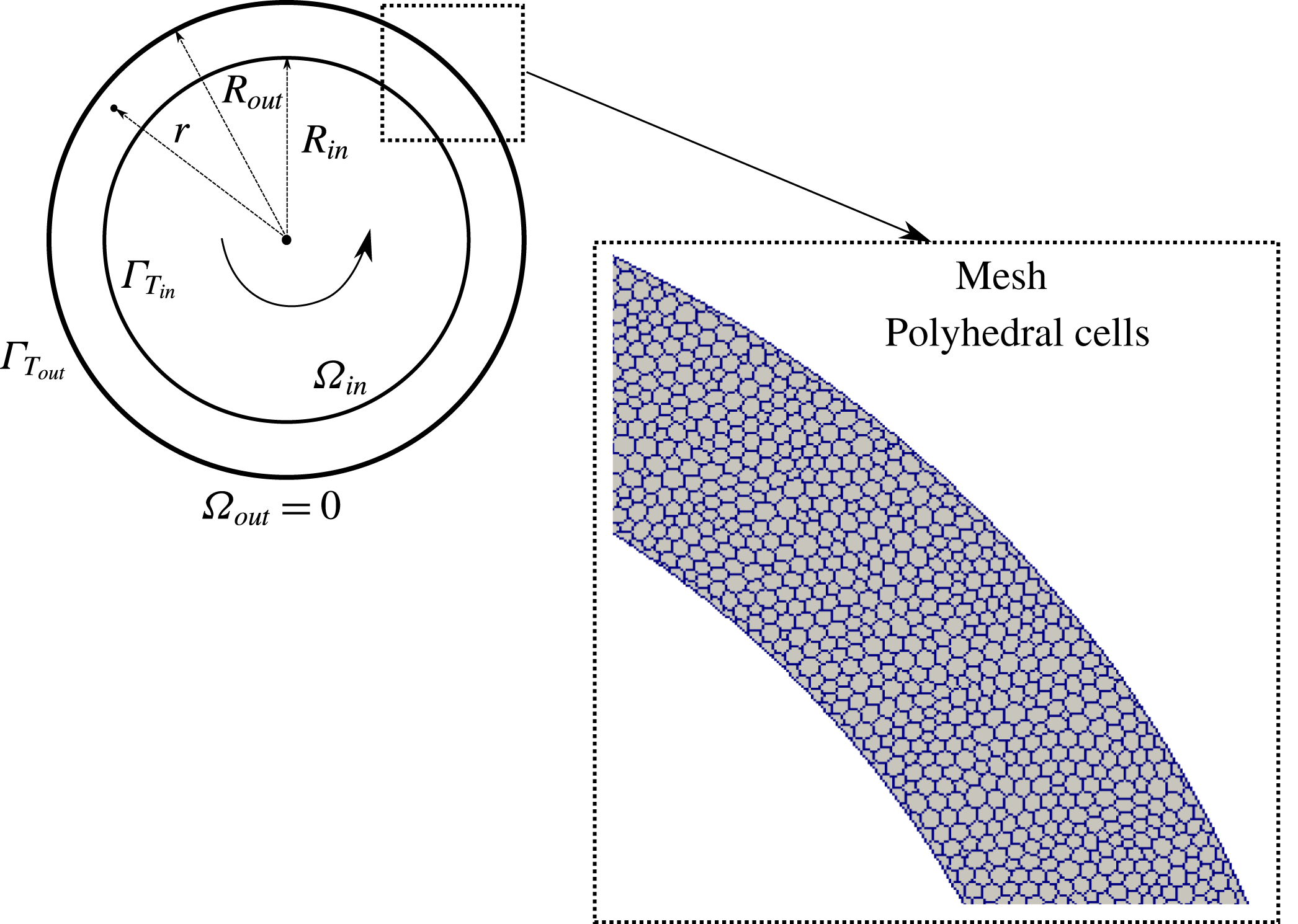
) as shown in figure 1 in a vertical Couette cell 12 mm in gap. The local shear rate
 $\dot{\unicode[STIX]{x1D6FE}}(r)$
in the Couette cell is given by:
 $$\begin{eqnarray}\dot{\unicode[STIX]{x1D6FE}}(r)=2\unicode[STIX]{x1D6FA}_{in}\left(\frac{R_{in}^{2}R_{out}^{2}}{R_{out}^{2}-R_{in}^{2}}\right)\frac{1}{r^{2}};\quad R_{in}\leqslant r\leqslant R_{out}.\end{eqnarray}$$
Couette cell geometry and mesh type.

The Couette cell was made of two copper wall cylinders and an experimental protocol of pulse heating was applied as the following: Metzger et al. (Reference Metzger, Rahli and Yin2013) first poured the suspension into the cell gap. The suspension was then thoroughly mixed at a large shear rate for 5 min. Then the shearing motion was stopped and Metzger et al. (Reference Metzger, Rahli and Yin2013) performed the reference experiment (suspension at rest): the inner cylinder was then heated for 5 s. Its typical temperature rise was
 $5\,^{\circ }\text{C}$
. Metzger et al. (Reference Metzger, Rahli and Yin2013) then let its temperature relax back to the room temperature
 $T_{atm}$
. Throughout this process the temperature of the inner cylinder was measured. Metzger et al. (Reference Metzger, Rahli and Yin2013) experiments were then performed at the desired shear rates
 $\dot{\unicode[STIX]{x1D6FE}}$
.
In order to reproduce numerically the pulse-heating experimental boundary conditions of Metzger et al. (Reference Metzger, Rahli and Yin2013) (i.e. the rise of
 $5\,^{\circ }\text{C}$
of the inner cylinder), the following Dirichlet and Neumann numerical boundary conditions are applied (see figure 1):
 $$\begin{eqnarray}\displaystyle & {\unicode[STIX]{x1D6E4}_{T}}_{in}\equiv (T_{in}=298~\text{K});\quad \unicode[STIX]{x1D6FA}_{in}=0;\quad {\unicode[STIX]{x1D6E4}_{T}}_{out}\equiv (\unicode[STIX]{x1D735}T\boldsymbol{\cdot }\boldsymbol{n}=0);\quad \text{if}~t\leqslant 5~\text{s} & \displaystyle\end{eqnarray}$$
 $$\begin{eqnarray}\displaystyle & {\unicode[STIX]{x1D6E4}_{T}}_{in}\equiv (\unicode[STIX]{x1D735}T\boldsymbol{\cdot }\boldsymbol{n}=0);\quad \unicode[STIX]{x1D6FA}_{in}\neq 0;\quad {\unicode[STIX]{x1D6E4}_{T}}_{out}\equiv (\unicode[STIX]{x1D735}T\boldsymbol{\cdot }\boldsymbol{n}=0);\quad \text{if}~t>5~\text{s}. & \displaystyle\end{eqnarray}$$
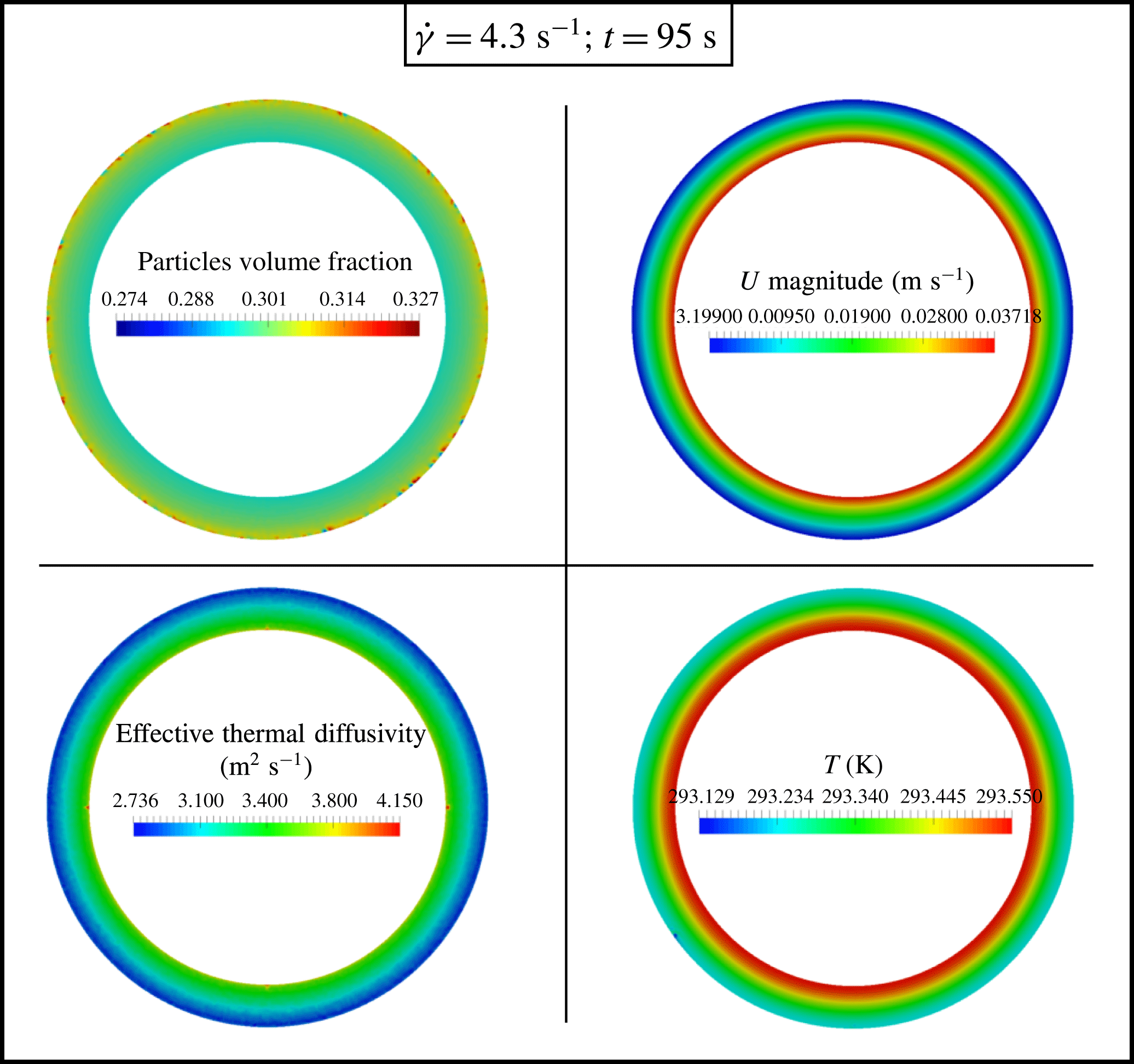
An example of the obtained CFD results for the local volume fraction
 $\unicode[STIX]{x1D719}$
, the suspension velocity magnitude, the temperature and the effective suspension thermal diffusivity are shown in figure 2.
Couette cell numerical results at
 $t=95$
s and
 $\dot{\unicode[STIX]{x1D6FE}}=4.3~\text{s}^{-1}$
. The applied simulation data are:
 $\unicode[STIX]{x1D719}_{bulk}=30\,\%$
;
 $n=1$
;
 $C_{1}=0$
;
 $d_{p}=2$
mm;
 ${\unicode[STIX]{x1D702}_{f}}_{i}=25.4\times 10^{-4}~\text{m}^{2}~\text{s}^{-1}$
;
 ${T_{f}}_{i}=293$
K;
 $\unicode[STIX]{x1D6FD}_{0}=10^{-3}~\text{K}^{-1}$
;
 $\unicode[STIX]{x1D70C}_{f}=\unicode[STIX]{x1D70C}_{p}=1180~\text{Kg}~\text{m}^{-3}$
;
 $C_{p_{f}}=C_{p_{p}}=1.26~\text{KJ}~\text{Kg}^{-1}~\text{K}^{-1}$
;
 $k_{f}=k_{p}=0.19~\text{W}~\text{m}^{-1}~\text{K}^{-1}$
.

Temperature decay of the inner cylinder. The applied simulation data are:
 $\unicode[STIX]{x1D719}_{bulk}=30\,\%$
;
 $n=1$
;
 $C_{1}=0$
;
 $d_{p}=2$
mm;
 ${\unicode[STIX]{x1D702}_{f}}_{i}=25.4\times 10^{-4}~\text{m}^{2}~\text{s}^{-1}$
;
 ${T_{f}}_{i}=293$
K;
 $\unicode[STIX]{x1D6FD}_{0}=10^{-3}~\text{K}^{-1}$
;
 $\unicode[STIX]{x1D70C}_{f}=\unicode[STIX]{x1D70C}_{p}=1180~\text{Kg}~\text{m}^{-3}$
;
 $C_{p_{f}}=C_{p_{p}}=1.26~\text{KJ}~\text{Kg}^{-1}~\text{K}^{-1}$
;
 $k_{f}=k_{p}=0.19~\text{W}~\text{m}^{-1}~\text{K}^{-1}$
.

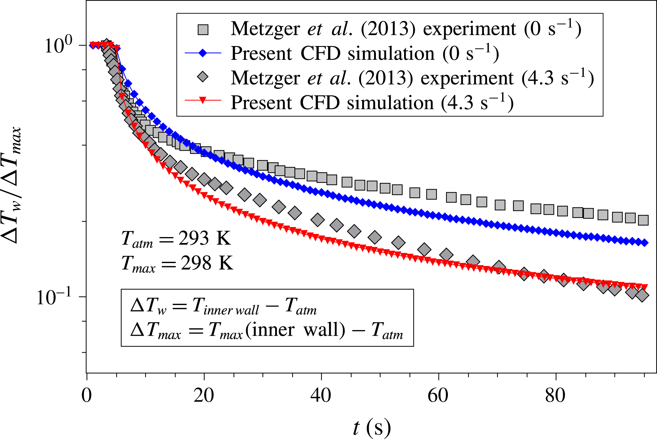
Figure 3 shows the present obtained CFD numerical results compared to the experimental ones obtained by Metzger et al. (Reference Metzger, Rahli and Yin2013) for
 $\dot{\unicode[STIX]{x1D6FE}}=0~\text{s}^{-1}$
and
 $\dot{\unicode[STIX]{x1D6FE}}=4.3~\text{s}^{-1}$
. At zero shear rate, a slight difference between the experimental and numerical linear–log profiles can be observed. This is due to different values in the effective thermal diffusivity
 $\unicode[STIX]{x1D6FC}_{0}$
of the suspension at rest. In the present work
 $\unicode[STIX]{x1D6FC}_{0}$
is approximately
 $3.23\times 10^{-7}~\text{m}^{2}~\text{s}^{-1}$
while in Metzger et al. (Reference Metzger, Rahli and Yin2013)
 $\unicode[STIX]{x1D6FC}_{0}$
was approximately
 $1.60\times 10^{-7}~\text{m}^{2}~\text{s}^{-1}$
. At
 $\dot{\unicode[STIX]{x1D6FE}}=4.3~\text{s}^{-1}$
, the numerical and experimental profiles are closer to each other and follow the following decay-law behaviour:
 $$\begin{eqnarray}\frac{T_{w}}{T_{inner\,\,wall}}=\frac{\unicode[STIX]{x0394}T_{w}}{\unicode[STIX]{x0394}T_{inner\,\,wall}}=\text{e}^{-A\sqrt{t}},\end{eqnarray}$$
where
 $\unicode[STIX]{x0394}T_{w}=(T_{w}-T_{atm})$
,
 $\unicode[STIX]{x0394}T_{inner\,\,wall}=(T_{inner\,\,wall}-T_{atm})$
,
 $A$
is a fitting constant parameter and
 $t$
is time. Metzger et al. (Reference Metzger, Rahli and Yin2013) showed in detail that the suspension effective thermal diffusivity
 $\unicode[STIX]{x1D6FC}^{\ast }$
can be computed at different shear-rate values using:
 $$\begin{eqnarray}\unicode[STIX]{x1D6FC}^{\ast }=\frac{\unicode[STIX]{x1D6FC}}{\unicode[STIX]{x1D6FC}_{0}}=\left(\frac{A}{A_{0}}\right)^{2},\end{eqnarray}$$
with
 $\unicode[STIX]{x1D6FC}_{0}$
and
 $A_{0}$
denoting the normalizing values computed at zero shear rate (suspension at rest).
Figure 3 illustrates that the CFD constitutive model in this work is able to capture the transient temperature decay of the inner cylinder. Moreover, it shows that shear, and thus SIM, have an influence on the suspension effective heat transfer properties.
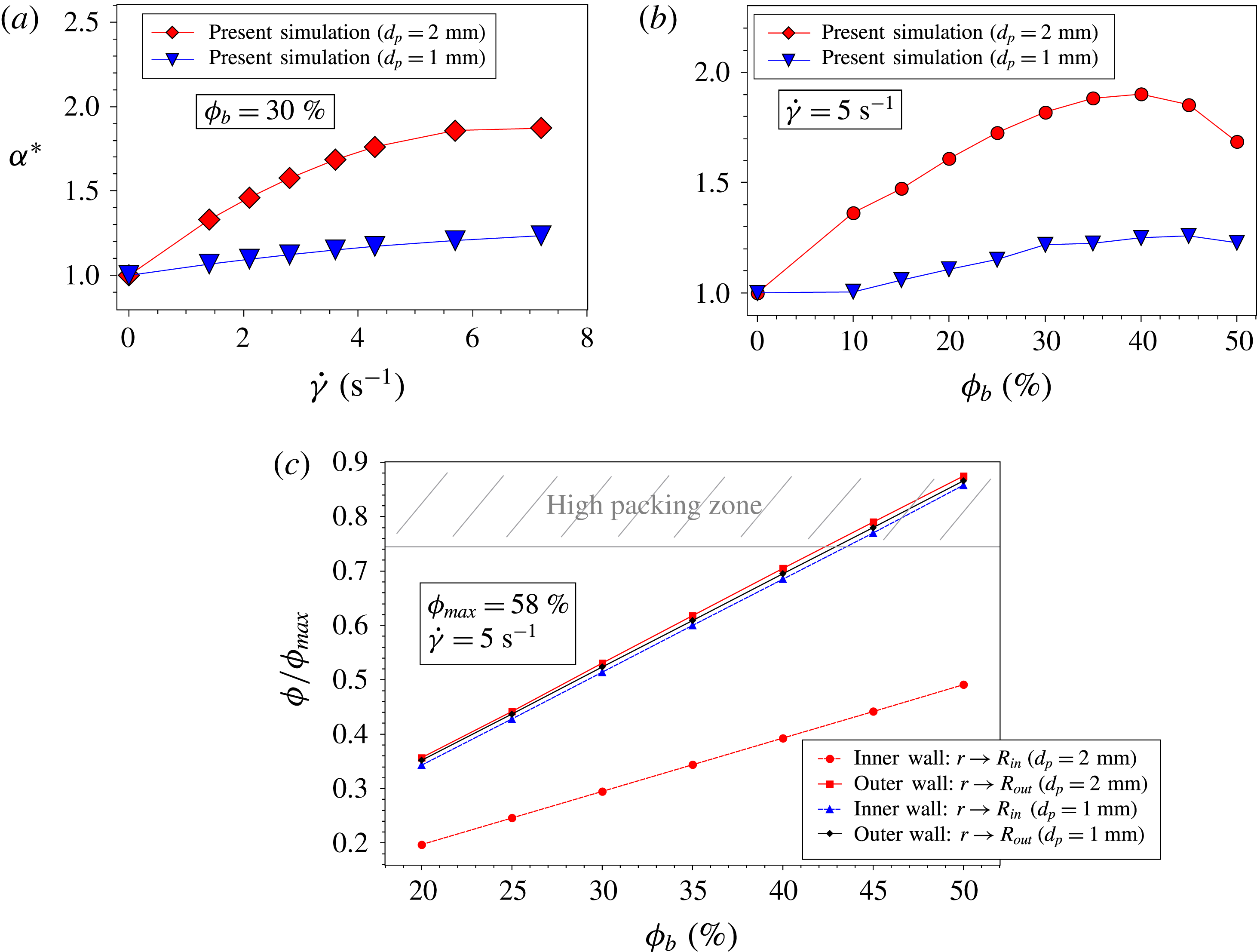
The numerical results for the influence of the local shear rate on the suspension effective thermal diffusivity are presented in figure 4(a). For particles of
 $d_{p}=1$
mm, a linear behaviour of
 $\unicode[STIX]{x1D6FC}^{\ast }$
is observed for all
 $\dot{\unicode[STIX]{x1D6FE}}=(0{-}7.2)~\text{s}^{-1}$
. However for particles of
 $d_{p}=2$
mm, an increasing linear behaviour of
 $\unicode[STIX]{x1D6FC}^{\ast }$
is observed for
 $\dot{\unicode[STIX]{x1D6FE}}=(0{-}5)~\text{s}^{-1}$
which is then damped around
 $\dot{\unicode[STIX]{x1D6FE}}>5~\text{s}^{-1}$
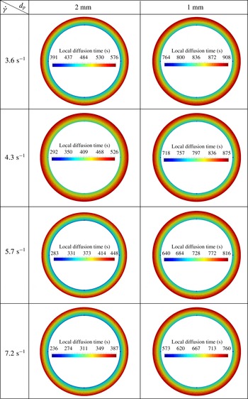
. This damping was also observed experimentally by Metzger et al. (Reference Metzger, Rahli and Yin2013) being an effect of the outer wall. For better illustration, figure 5 shows the local thermal diffusion time in the Couette cell gap. For 2 mm particles, figure 5 shows that the diffusion time required, so that heat propagates toward the exterior cylinder, decreases strongly with the increase in the shear rate. Moreover, this diffusion time at the exterior wall cylinder for 2 mm particles is lower than that for 1 mm particles.
Numerical results showing the influence of both the shear rate and the bulk volume fraction on the suspension effective thermal properties: (a) the suspension effective thermal diffusivity
 $\unicode[STIX]{x1D6FC}^{\ast }$
versus the applied shear rate
 $\dot{\unicode[STIX]{x1D6FE}}$
; (b) the suspension effective thermal diffusivity
 $\unicode[STIX]{x1D6FC}^{\ast }$
versus the bulk volume fraction
 $\unicode[STIX]{x1D719}_{bulk}$
; (c) the normalized local volume fraction
 $\unicode[STIX]{x1D719}/\unicode[STIX]{x1D719}_{max}$
as function of the bulk volume fraction
 $\unicode[STIX]{x1D719}_{bulk}$
. The applied simulation data are:
 $n=1$
;
 $C_{1}=0$
;
 ${\unicode[STIX]{x1D702}_{f}}_{i}=25.4\times 10^{-4}~\text{m}^{2}~\text{s}^{-1}$
;
 ${T_{f}}_{i}=293$
K;
 $\unicode[STIX]{x1D6FD}_{0}=10^{-3}~\text{K}^{-1}$
;
 $\unicode[STIX]{x1D70C}_{f}=\unicode[STIX]{x1D70C}_{p}=1180~\text{Kg}~\text{m}^{-3}$
;
 $C_{p_{f}}=C_{p_{p}}=1.26~\text{KJ}~\text{Kg}^{-1}~\text{K}^{-1}$
;
 $k_{f}=k_{p}=0.19~\text{W}~\text{m}^{-1}~\text{K}^{-1}$
.

Local thermal diffusion time in seconds versus
 $\dot{\unicode[STIX]{x1D6FE}}$
and
 $d_{p}$
. The applied simulation data are:
 $\unicode[STIX]{x1D719}_{bulk}=30\,\%$
;
 $n=1$
;
 $C_{1}=0$
;
 ${\unicode[STIX]{x1D702}_{f}}_{i}=25.4\times 10^{-4}~\text{m}^{2}~\text{s}^{-1}$
;
 ${T_{f}}_{i}=293$
K;
 $\unicode[STIX]{x1D6FD}_{0}=10^{-3}~\text{K}^{-1}$
;
 $\unicode[STIX]{x1D70C}_{f}=\unicode[STIX]{x1D70C}_{p}=1180~\text{Kg}~\text{m}^{-3}$
;
 $C_{p_{f}}=C_{p_{p}}=1.26~\text{KJ}~\text{Kg}^{-1}~\text{K}^{-1}$
;
 $k_{f}=k_{p}=0.19~\text{W}~\text{m}^{-1}~\text{K}^{-1}$
.

The influence of the numerical bulk volume fraction on the suspension effective thermal diffusivity is presented in figure 4(b) at
 $5~\text{s}^{-1}$
shear-rate value. For particles of both
 $d_{p}=1$
mm and
 $d_{p}=2$
mm, an increasing linear behaviour in
 $\unicode[STIX]{x1D6FC}^{\ast }$
is observed for
 $\unicode[STIX]{x1D719}$
between 0 and 40 %. However for larger volume fraction values (
 $\unicode[STIX]{x1D719}>40\,\%$
), a decrease in
 $\unicode[STIX]{x1D6FC}^{\ast }$
is observed for particles of
 $d_{p}=2$
mm, while a saturation in
 $\unicode[STIX]{x1D6FC}^{\ast }$
is observed for particles of
 $d_{p}=1$
mm. The decrease behaviour predicted by the present CFD model in figure 4(b) was also observed experimentally be Metzger et al. (Reference Metzger, Rahli and Yin2013) who explained and showed that this is an important feature that occurs at large
 $\unicode[STIX]{x1D719}$
values. Metzger et al. (Reference Metzger, Rahli and Yin2013) illustrated that this behaviour is due to the particle diffusion coefficients that dramatically decrease with increasing
 $\unicode[STIX]{x1D719}$
both in experiments and simulations where a substantial change in the particle microstructure is observed: particles organize into layers. Figure 4(c) shows the present CFD modelling results for the normalized local volume fraction
 $\unicode[STIX]{x1D719}/\unicode[STIX]{x1D719}_{max}$
values as function of
 $\unicode[STIX]{x1D719}_{bulk}$
. These simulation results were taken after
 $t_{total}=90$
s. In agreement with the findings of Metzger et al. (Reference Metzger, Rahli and Yin2013), it can be observed that for 2 mm particles, migration towards the exterior cylinder is important and a high packing zone is reached around
 $\unicode[STIX]{x1D719}>40\,\%$
as a result of particles being more compacted/concentrated near the outer cylinder wall. However, for 1 mm particles migration was almost absent.
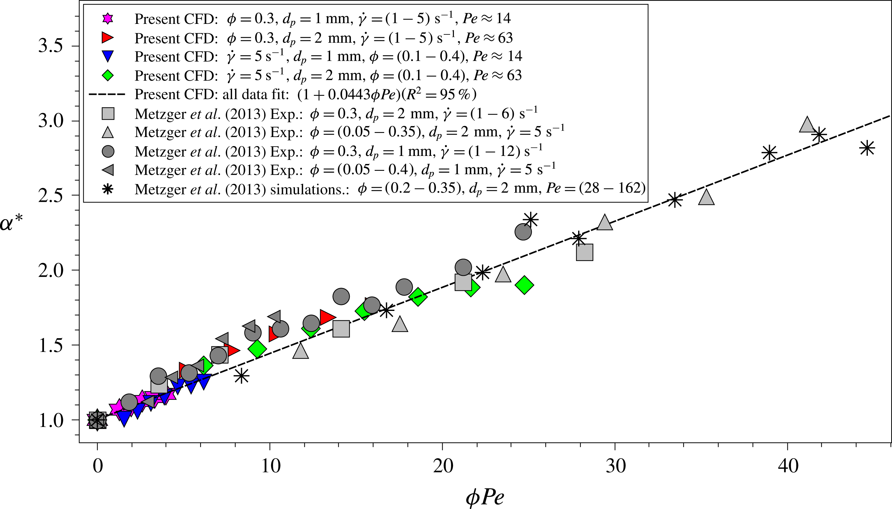
Figure 6 shows all the present CFD numerical results of
 $\unicode[STIX]{x1D6FC}^{\ast }$
as function of
 $\unicode[STIX]{x1D719}Pe$
. As observed experimentally and numerically by Metzger et al. (Reference Metzger, Rahli and Yin2013), for moderate
 $Pe<100$
, it can be seen from figure 6 that the present CFD modelling approach is able to recover a linear behaviour of
 $\unicode[STIX]{x1D6FC}^{\ast }$
versus
 $\unicode[STIX]{x1D719}~Pe$
that satisfies well the constitutive formulation presented in (2.13) with
 $\unicode[STIX]{x1D6FD}\approx 0.044$
(close to
 $\unicode[STIX]{x1D6FD}=0.046$
).
Suspension effective thermal diffusivity versus
 $\unicode[STIX]{x1D719}Pe$
. The applied simulation data are:
 $n=1$
;
 $C_{1}=0$
;
 ${\unicode[STIX]{x1D702}_{f}}_{i}=25.4\times 10^{-4}~\text{m}^{2}~\text{s}^{-1}$
;
 ${T_{f}}_{i}=293$
K;
 $\unicode[STIX]{x1D6FD}_{0}=10^{-3}~\text{K}^{-1}$
;
 $\unicode[STIX]{x1D70C}_{f}=\unicode[STIX]{x1D70C}_{p}=1180~\text{Kg}~\text{m}^{-3}$
;
 $C_{p_{f}}=C_{p_{p}}=1.26~\text{KJ}~\text{Kg}^{-1}~\text{K}^{-1}$
;
 $k_{f}=k_{p}=0.19~\text{W}~\text{m}^{-1}~\text{K}^{-1}$
.

4.2 Enhancement of heat transfer in rectangular channel by using non-colloidal laminar forced-convection suspension flow
4.2.1 Suspension flow type and geometry
The validated developed 3-D CFD model is applied here to a forced-convection isodense suspension laminar flow (
 $Re=10$
,
 $Ri=Gr_{D_{h}}Re^{-2}\ll 1$
,
 $Pr=\unicode[STIX]{x1D702}_{S}/\unicode[STIX]{x1D6FC}_{S}\sim O(10^{3})$
) inside a 3-D rectangular channel of square cross-section (3-D transient simulations).
 $Re$
is the suspension effective Reynolds number such that
 $Re=U_{m}d_{p}/\unicode[STIX]{x1D702}_{S}$
with
 $U_{m}$
being the suspension mass-averaged velocity in the flow direction
 $x$
. The channel walls, made of copper, are all at a constant imposed
 $T_{W}=323$
K while the flow enters the channel at
 $T_{in}=293$
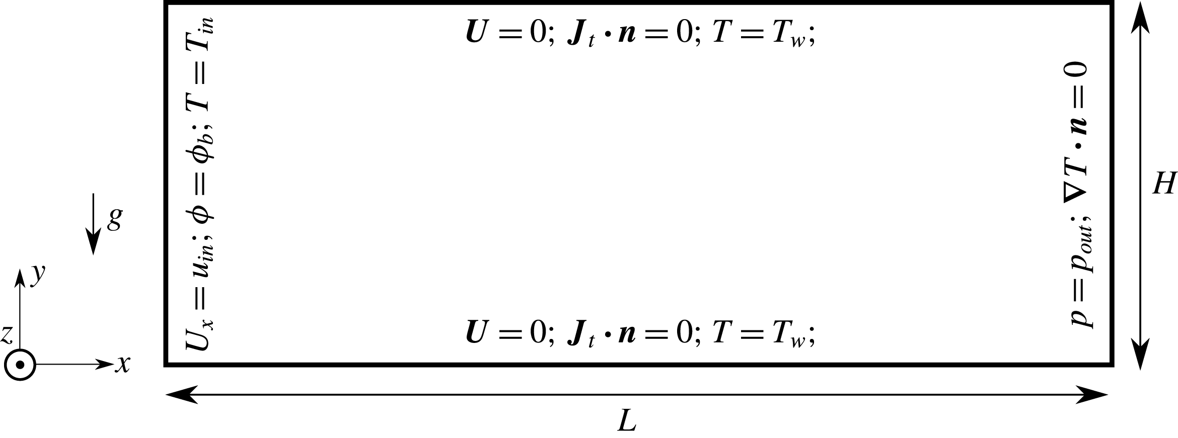
K as shown at the upper side of figure 7. A high aspect ratio
 $\unicode[STIX]{x1D709}=L/D_{h}=800$
was chosen after estimating both the effective hydrodynamic and thermal entrance lengths
 $x_{hd}$
and
 $x_{th}$
, respectively.
 $D_{h}$
denotes the channel’s hydraulic diameter
 $D_{h}=H=5$
mm and the suspension is of
 $\unicode[STIX]{x1D719}_{bulk}=35\,\%$
and
 $d_{p}=100~\unicode[STIX]{x03BC}\text{m}$
.
The numerical boundary conditions are shown at the lower side of figure 7 such that a Dirichlet type boundary condition for velocity, temperature and concentration are all applied at the entry. A Dirichlet type boundary condition for pressure and a Neumann type boundary condition for temperature and concentration are all applied at the outlet. At the channel walls, constant uniform
 $\boldsymbol{U}=0$
and
 $T=T_{w}$
are imposed for velocity and temperature, while Neumann type boundary condition is applied for the total migration flux (so that zero particles penetrate the walls).
The geometry of the channel with its boundary conditions applied at the inlet, outlet and walls.
 $\boldsymbol{n}$
represents the unit vector normal to the boundary surface.

The local Nusselt number for a suspension flow in a channel is defined as the following:
 $$\begin{eqnarray}{Nu_{x}}_{S}={h_{x}}_{S}D_{h}/k_{S},\end{eqnarray}$$
where
 ${h_{x}}_{S}$
is the suspension effective heat transfer coefficient along the channel dimensionless length (
 $x^{\ast }=x/(D_{h}RePr)$
).
For cases of constant temperature boundary condition applied at the channel exterior walls, following Shah & London (Reference Shah and London1974, Reference Shah and London1978), the effective
 ${Nu_{x}}_{S}$
for a suspension can be calculated as the following:
 $$\begin{eqnarray}{Nu_{x}}_{S}=\frac{D_{h}^{2}{U_{m}}_{S}(x)}{4\unicode[STIX]{x1D6FC}_{S}(T_{W}-{T_{m}}_{S}(x))},\end{eqnarray}$$
where
 ${U_{m}}_{S}(x)$
and
 ${T_{m}}_{S}(x)$
are the mass-flow-averaged velocity and the mass-averaged suspension temperature, respectively (at a position
 $x$
from entry in the flow direction). A mass-flow-averaged quantity
 $q_{m}(x)$
at a channel’s local section position
 $x$
of cross-section total area
 $A_{c}$
is computed as the following:
 $$\begin{eqnarray}q_{m}=\frac{\displaystyle \int _{A_{c}}q\unicode[STIX]{x1D70C}|\boldsymbol{U}\boldsymbol{\cdot }\text{d}\boldsymbol{A}_{\boldsymbol{c}}|}{\displaystyle \int _{A_{c}}\unicode[STIX]{x1D70C}|\boldsymbol{U}\boldsymbol{\cdot }\text{d}\boldsymbol{A}_{\boldsymbol{c}}|}=\frac{\displaystyle \mathop{\sum }_{i=1}^{n_{cells}}q_{i}\unicode[STIX]{x1D70C}_{i}|\boldsymbol{U}_{i}\boldsymbol{\cdot }\boldsymbol{A}_{\boldsymbol{c}_{i}}|}{\displaystyle \mathop{\sum }_{i=1}^{n_{cells}}\unicode[STIX]{x1D70C}_{i}|\boldsymbol{U}_{i}\boldsymbol{\cdot }\boldsymbol{A}_{\boldsymbol{c}_{i}}|},\end{eqnarray}$$
where
 $n_{cells}$
represents the total number of facets constituting the total surface area
 $A_{c}$
at a local channel’s cross-section. A structured non-uniform hexahedral mesh of cells is used to discretize the present 3-D channel of figure 7. A fine mesh is used with mesh refinement applied from the entry to the exit of the channel.
4.2.2 Influence of the conductivity ratio
To verify and justify the correct choice of our final valid 3-D mesh (i.e. size, type, refinement at entry, etc.) and the corresponding numerical schemes, first
 ${Nu_{x}}_{S}(\unicode[STIX]{x1D719}_{bulk}=0)$
is computed and compared to previously computed local steady Nusselt number
 ${Nu_{x}}_{f}$
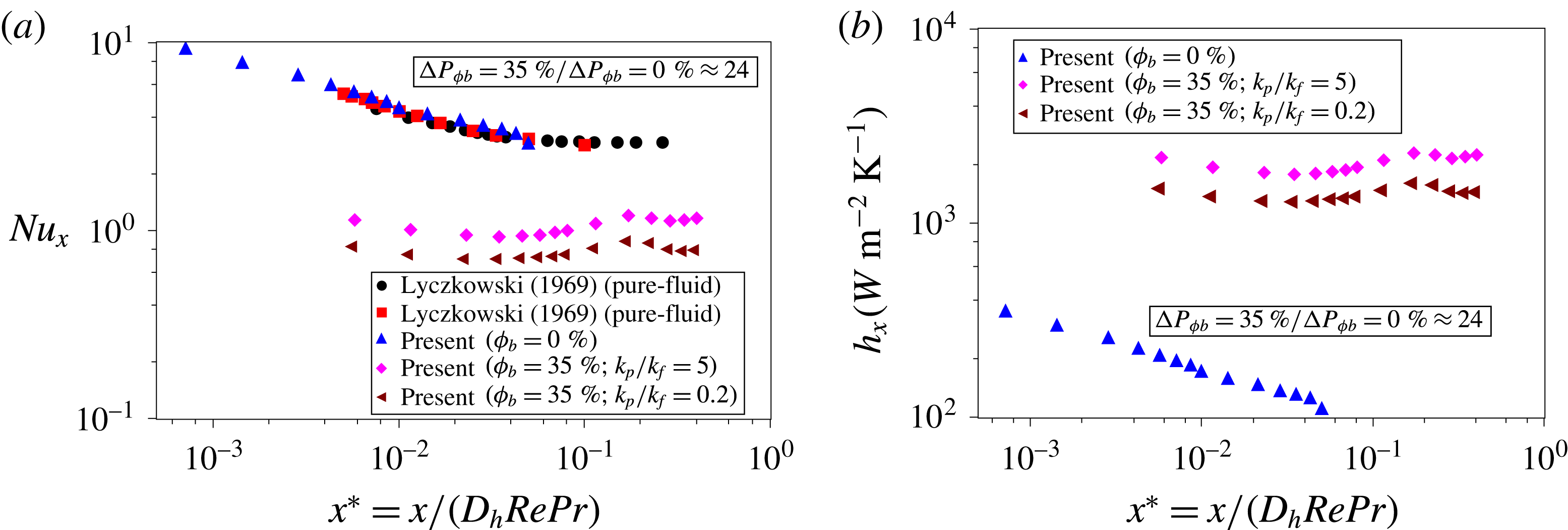
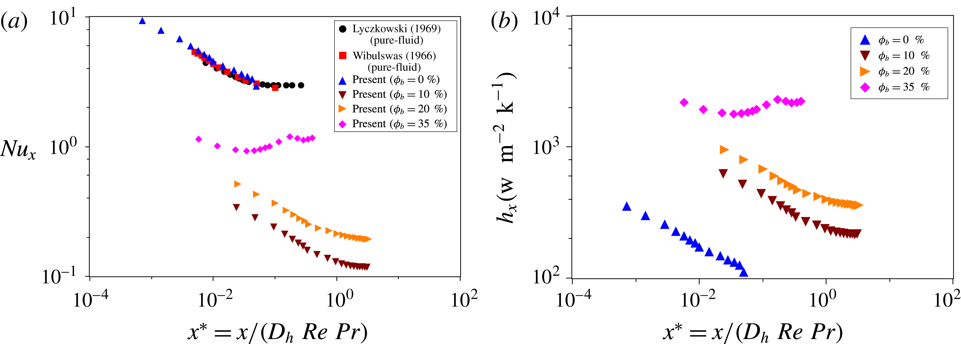
profiles obtained from the literature by Wibulswas (Reference Wibulswas1966), Lyczkowski, Solbirg & Gidaspow (Reference Lyczkowski, Solbirg and Gidaspow1969) (for fully developed velocity profiles of a pure fluid laminar flow in a square cross-section channel). This is shown in figure 8(a) where a good match is obtained compared to the results of Wibulswas (Reference Wibulswas1966) and Lyczkowski et al. (Reference Lyczkowski, Solbirg and Gidaspow1969). Then, two new simulation cases at
 $k_{p}/k_{f}=5$
and
 $0.2$
are conducted and the steady
 ${Nu_{x}}_{S}(\unicode[STIX]{x1D719}_{bulk}=35\,\%)$
values are obtained and presented in figure 8(a). The overall heat transfer enhancement is well characterized and can be seen from figure 8(b) where the overall steady effective heat transfer coefficient is very well augmented.
Local heat transfer properties: (a) local Nusselt number along the flow direction; (b) local heat transfer coefficient along the flow direction. The applied simulation data are:
 $\unicode[STIX]{x1D719}_{bulk}=35\,\%$
;
 $n=1$
;
 $C_{1}=2.3$
;
 $C_{2}=50$
K;
 $T_{c}=180$
K;
 $d_{p}=100~\unicode[STIX]{x03BC}\text{m}$
;
 ${\unicode[STIX]{x1D702}_{f}}_{i}=8\times 10^{-7}~\text{m}^{2}~\text{s}^{-1}$
;
 ${T_{f}}_{i}=293$
K;
 $\unicode[STIX]{x1D6FD}_{0}=3\times 10^{-4}~\text{K}^{-1}$
;
 $\unicode[STIX]{x1D70C}_{f}=\unicode[STIX]{x1D70C}_{p}=1180~\text{Kg}~\text{m}^{-3}$
;
 $C_{p_{f}}=C_{p_{p}}\approx 1~\text{KJ}~\text{Kg}^{-1}~\text{K}^{-1}$
.

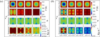
Figures 9(a) and 9(b) show the obtained numerical CFD results represented by snapshots taken at four different cross-section locations along the flow direction (at the steady state) for
 $k_{p}/k_{f}=5$
and
 $k_{p}/k_{f}=0.2$
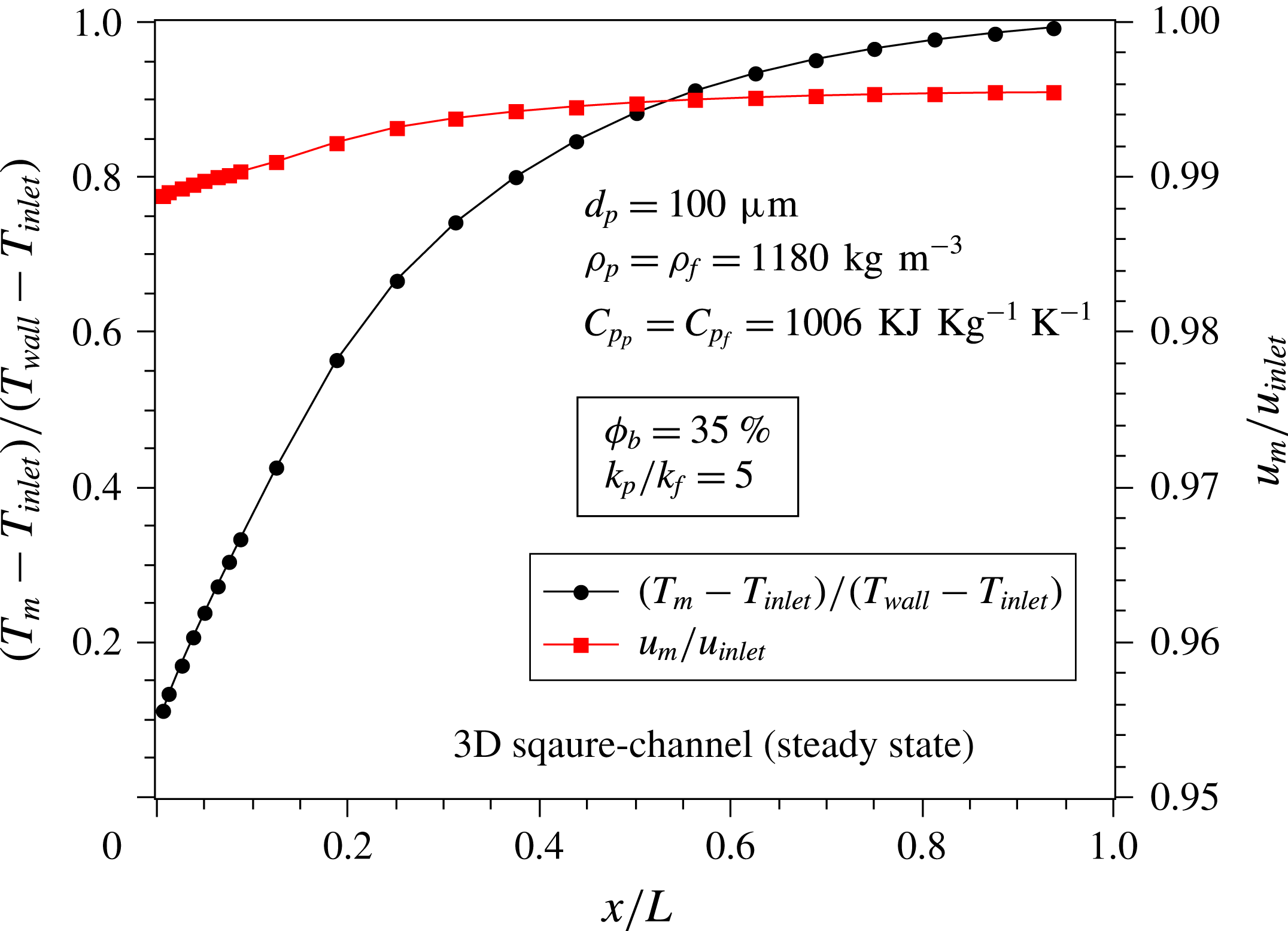
, respectively. Figure 9 illustrates clearly that the suspension temperature overall values in the cross-section from the channel’s entry to the channel’s exit are higher than those observed in the case of a pure fluid flow. Figure 10 shows local information about the mass-flow-averaged temperature and the streamwise velocity in the cross-section along the channel’s length at steady state. Compared to pure fluid flow, it is observed that heat transfer enhancement may be achieved by applying a dense suspension flow with an implicit contribution to this heat transfer from both the local SIM of particles and slight buoyancy effects. In this case, buoyancy effects are considered in the 3-D example but they have a very small effect. Similar initial density values were imposed for both the particles and the fluid, but the fluid density changes slightly due to the change in temperature; however, the particle density (due to considering rigid particles in our modelling approach) remains constant. Since the fluid density changes and the particle density does not, a non-negligible
 $\unicode[STIX]{x0394}\unicode[STIX]{x1D70C}$
is induced in the suspension flow explaining the break in the suspension flow axisymmetry with respect to the centre of the cross-section (compared to the pure fluid case). One should not forget also the presence of the suspension flow circulations due to the four sharp corner edges of the square cross-section where more particles are observed to be entrapped (higher volume fraction values).
Snapshots at four different cross-section locations along the flow direction at the steady state: (a) results for
 $k_{p}/k_{f}=5$
; (b) results for
 $k_{p}/k_{f}=0.2$
. The initially applied simulation data are:
 $\unicode[STIX]{x1D719}_{bulk}=35\,\%$
;
 $n=1$
;
 $C_{1}=2.3$
;
 $C_{2}=50$
K;
 $T_{c}=180$
K;
 $d_{p}=100~\unicode[STIX]{x03BC}\text{m}$
;
 ${\unicode[STIX]{x1D702}_{f}}_{i}=8\times 10^{-7}~\text{m}^{2}~\text{s}^{-1}$
;
 ${T_{f}}_{i}=293$
K;
 $\unicode[STIX]{x1D6FD}_{0}=3\times 10^{-4}~\text{K}^{-1}$
;
 $\unicode[STIX]{x1D70C}_{f}=\unicode[STIX]{x1D70C}_{p}=1180~\text{Kg}~\text{m}^{-3}$
;
 $C_{p_{f}}=C_{p_{p}}\approx 1~\text{KJ}~\text{Kg}^{-1}~\text{K}^{-1}$
.

In order to quantify well the global heat transfer enhancement in channels by using suspension flows, a suspension thermal enhancement global factor (STEF) is defined as a function of the initial
 $\unicode[STIX]{x1D719}_{bulk}$
(i.e.
 $\bar{Nu}$
results from integrating the
 $Nu_{x}$
number along the channel’s length in the flow direction
 $x$
). It is given as the following:
 $$\begin{eqnarray}\text{STEF}(\unicode[STIX]{x1D719}_{bulk})=\left(\frac{\bar{Nu}_{S}(0\,\%)}{\bar{Nu_{S}}(\unicode[STIX]{x1D719}_{bulk})}\right)\left(\frac{f_{S}(\unicode[STIX]{x1D719}_{bulk})}{f_{S}(0\,\%)}\right)^{-1/3},\end{eqnarray}$$
where
 $f_{S}$
is the suspension effective friction coefficient (to account for pressure drop) given by:
 $$\begin{eqnarray}f_{S}=\frac{\unicode[STIX]{x0394}p}{\unicode[STIX]{x1D709}\unicode[STIX]{x1D70C}_{S}U_{m}^{2}}.\end{eqnarray}$$
Using (4.9) and (4.10), it is found that
 $\text{STEF}>1$
with (
 $\text{STEF}(35\,\%)=6.04$
for
 $k_{p}/k_{f}=5$
) and (
 $\text{STEF}(35\,\%)=8.28$
for
 $k_{p}/k_{f}=0.2$
) for suspensions having (
 $d_{p}=100~\unicode[STIX]{x03BC}\text{m}$
;
 $\unicode[STIX]{x1D70C}_{f}=\unicode[STIX]{x1D70C}_{p}$
;
 ${C_{p}}_{f}={C_{p}}_{p}$
). The
 $\text{STEF}>1$
means a good overall thermal enhancement induced by the dense suspension flow. Figure 9(b) shows results at four different cross-section locations along the flow direction. It can be clearly seen that suspension flow contributes to additional heat transfer and mixing inside the channel.
Looking back to figure 8(b), one may observe a slight increase–decrease behaviour in
 $h_{x}$
at around
 $x^{\ast }\approx 0.1$
(similarly for
 $Nu_{x}$
in figure 8
a). This can be explained by the fact that the suspension flow is developing (dynamically and thermally) along the channel’s length and starts to stabilize after a cross-section position of
 $x/L\approx 0.4$
corresponding to
 $x^{\ast }\approx 0.1$
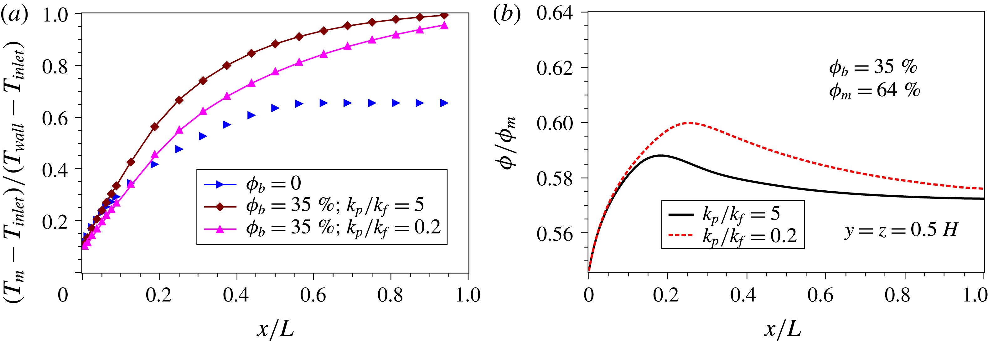
. This can be better explained by looking to figure 11 where these dynamical and thermal suspension flow development behaviours occur. Figures 11(a) and 11(b) show respectively that the mass-flow-averaged dimensionless temperature, and the local concentration are developing towards more stable stationary values after
 $x/L\approx 0.4$
(
 $\equiv x^{\ast }\approx 0.1$
) along the channel’s length. This demonstrates the influence of the shear-induced migration on heat transfer at the steady state of the suspension flow inside the channel.
Dimensionless mass-flow-averaged temperature and streamwise velocity in the cross-section along the channel’s length at steady state for suspension at
 $\unicode[STIX]{x1D719}_{b}=35\,\%$
and
 $k_{p}/k_{f}=5$
. The initially applied simulation data are:
 $\unicode[STIX]{x1D719}_{bulk}=35\,\%$
;
 $n=1$
;
 $C_{1}=2.3$
;
 $C_{2}=50$
K;
 $T_{c}=180$
K;
 $d_{p}=100~\unicode[STIX]{x03BC}\text{m}$
;
 ${\unicode[STIX]{x1D702}_{f}}_{i}=8\times 10^{-7}~\text{m}^{2}~\text{s}^{-1}$
;
 ${T_{f}}_{i}=293$
K;
 $\unicode[STIX]{x1D6FD}_{0}=3\times 10^{-4}~\text{K}^{-1}$
;
 $\unicode[STIX]{x1D70C}_{f}=\unicode[STIX]{x1D70C}_{p}=1180~\text{Kg}~\text{m}^{-3}$
;
 $C_{p_{f}}=C_{p_{p}}\approx 1~\text{KJ}~\text{Kg}^{-1}~\text{K}^{-1}$
.

Moreover, figure 11(a) illustrates that the mass-flow-averaged dimensionless temperature reaches higher values at
 $\unicode[STIX]{x1D719}_{b}=35\,\%$
rather than at
 $\unicode[STIX]{x1D719}_{b}=0\,\%$
in the cross-section along the channel’s length. Moreover, for two different values of
 $k_{p}/k_{f}=5$
and
 $k_{p}/k_{f}=0.2$
, figure 11(b) shows different local volume fraction values obtained along the channel’s centreline of two suspensions both at
 $\unicode[STIX]{x1D719}_{b}=35\,\%$
. This explains the SIM contribution to the heat transfer enhancement and thus implicitly the mass-flow-averaged dimensionless temperature variations that was shown in figure 11(a).
Local temperature and volume fraction in the cross-section along the channel’s length at steady state for several
 $\unicode[STIX]{x1D719}_{b}$
and
 $k_{p}/k_{f}$
values: (a) local mass-flow-averaged dimensionless temperature; (b) normalized local volume fraction. The initially applied simulation data are:
 $n=1$
;
 $C_{1}=2.3$
;
 $C_{2}=50$
K;
 $T_{c}=180$
K;
 $d_{p}=100~\unicode[STIX]{x03BC}\text{m}$
;
 ${\unicode[STIX]{x1D702}_{f}}_{i}=8\times 10^{-7}~\text{m}^{2}~\text{s}^{-1}$
;
 ${T_{f}}_{i}=293$
K;
 $\unicode[STIX]{x1D6FD}_{0}=3\times 10^{-4}~\text{K}^{-1}$
;
 $\unicode[STIX]{x1D70C}_{f}=\unicode[STIX]{x1D70C}_{p}=1180~\text{Kg}~\text{m}^{-3}$
;
 $C_{p_{f}}=C_{p_{p}}\approx 1~\text{KJ}~\text{Kg}^{-1}~\text{K}^{-1}$
.

4.2.3 Influence of the initial bulk volume fraction
In this section we show the influence of the initial bulk volume fraction
 $\unicode[STIX]{x1D719}=\unicode[STIX]{x1D719}_{b}$
on the heat transfer by using the suspension flow in a channel at
 $k_{p}/k_{f}=5$
. Figure 12(a) shows that the local Nusselt number values decrease with the decrease in the initial bulk volume fraction of particles
 $\unicode[STIX]{x1D719}_{b}\neq 0$
, illustrating overall heat transfer enhancement compared to a pure fluid case at
 $\unicode[STIX]{x1D719}_{b}=0$
. Moreover a transitional behaviour is observed between moderate values of
 $\unicode[STIX]{x1D719}_{b}=10\,\%$
, 20 % and higher values of
 $\unicode[STIX]{x1D719}_{b}=35\,\%$
. For
 $\unicode[STIX]{x1D719}_{b}=10\,\%$
, 20 % the
 $Nu_{x}$
decreases with the increase of
 $x^{\ast }$
with a behaviour close to that in the case of pure fluid. However, for the dense suspension case of
 $\unicode[STIX]{x1D719}_{b}=35\,\%$
, the local Nusselt number
 $Nu_{x}$
tends to decrease slightly with the increase in
 $x^{\ast }$
with a slight sudden jump around
 $x^{\ast }$
between 0.1 and 0.15. This complex behaviour is difficult to explain and could be a result of higher interaction frequency among the immersed particles at high
 $\unicode[STIX]{x1D719}_{b}$
values of the suspension.
Local thermal properties at the steady state for different initial
 $\unicode[STIX]{x1D719}_{bulk}$
values: (a) local Nusselt number; (b) local heat transfer coefficient. The initially applied simulation data are:
 $k_{p}/k_{f}=5$
;
 $n=1$
;
 $C_{1}=2.3$
;
 $C_{2}=50$
K;
 $T_{c}=180$
K;
 $d_{p}=100~\unicode[STIX]{x03BC}\text{m}$
;
 ${\unicode[STIX]{x1D702}_{f}}_{i}=8\times 10^{-7}~\text{m}^{2}~\text{s}^{-1}$
;
 ${T_{f}}_{i}=293$
K;
 $\unicode[STIX]{x1D6FD}_{0}=3\times 10^{-4}~\text{K}^{-1}$
;
 $\unicode[STIX]{x1D70C}_{f}=\unicode[STIX]{x1D70C}_{p}=1180~\text{Kg}~\text{m}^{-3}$
;
 $C_{p_{f}}=C_{p_{p}}\approx 1~\text{KJ}~\text{Kg}^{-1}~\text{K}^{-1}$
.

To quantify the overall heat transfer, the local heat transfer coefficient
 $h_{x}$
values are computed. Figure 12(b) shows that the
 $h_{x}$
coefficient increases with the increase of the initial bulk volume fraction
 $\unicode[STIX]{x1D719}_{b}$
quantifying the heat transfer enhancement in channel by applying a suspension flow.
As is expected, the pressure drop value is found to increase with
 $\unicode[STIX]{x1D719}_{b}$
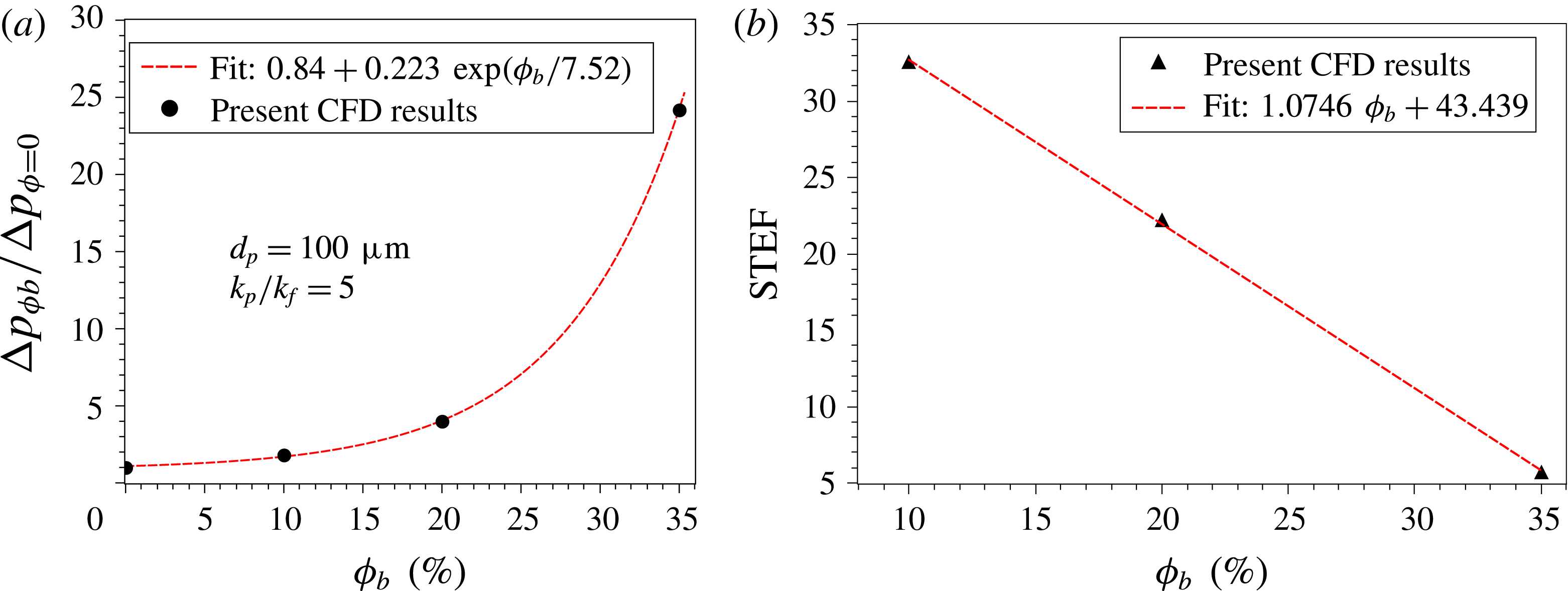
as shown in figure 13(a). For better quantification in terms of overall performance of the system, the overall suspension thermal enhancement factors (
 $\text{STEF}$
) of (4.9) were computed for the different
 $\unicode[STIX]{x1D719}_{b}$
values (10 %, 20 %, 35 %). Figure 13(b) shows that the
 $\text{STEF}$
values are all greater than unity, with higher values obtained at lower
 $\unicode[STIX]{x1D719}_{b}$
due to lower pressure drop values at lower bulk volume fraction of particles.
Thermal enhancement results at the steady state for different initial
 $\unicode[STIX]{x1D719}_{bulk}$
values: (a) dimensionless pressure drop; (b) suspension thermal enhancement factor. The initially applied simulation data are:
 $k_{p}/k_{f}=5$
;
 $n=1$
;
 $C_{1}=2.3$
;
 $C_{2}=50$
K;
 $T_{c}=180$
K;
 $d_{p}=100~\unicode[STIX]{x03BC}\text{m}$
;
 ${\unicode[STIX]{x1D702}_{f}}_{i}=8\times 10^{-7}~\text{m}^{2}~\text{s}^{-1}$
;
 ${T_{f}}_{i}=293$
K;
 $\unicode[STIX]{x1D6FD}_{0}=3\times 10^{-4}~\text{K}^{-1}$
;
 $\unicode[STIX]{x1D70C}_{f}=\unicode[STIX]{x1D70C}_{p}=1180~\text{Kg}~\text{m}^{-3}$
;
 $C_{p_{f}}=C_{p_{p}}\approx 1~\text{KJ}~\text{Kg}^{-1}~\text{K}^{-1}$
.

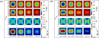
Snapshots at four different cross-section locations along the flow direction at the steady state for
 $k_{p}/k_{f}=5$
: (a) for
 $\unicode[STIX]{x1D719}_{b}=10\,\%$
; (b) for
 $\unicode[STIX]{x1D719}_{b}=20\,\%$
. The initially applied simulation data are:
 $n=1$
;
 $C_{1}=2.3$
;
 $C_{2}=50$
K;
 $T_{c}=180$
K;
 $d_{p}=100~\unicode[STIX]{x03BC}\text{m}$
;
 ${\unicode[STIX]{x1D702}_{f}}_{i}=8\times 10^{-7}~\text{m}^{2}~\text{s}^{-1}$
;
 ${T_{f}}_{i}=293$
K;
 $\unicode[STIX]{x1D6FD}_{0}=3\times 10^{-4}~\text{K}^{-1}$
;
 $\unicode[STIX]{x1D70C}_{f}=\unicode[STIX]{x1D70C}_{p}=1180~\text{Kg}~\text{m}^{-3}$
;
 $C_{p_{f}}=C_{p_{p}}\approx 1~\text{KJ}~\text{Kg}^{-1}~\text{K}^{-1}$
.

Figure 14 shows several results for
 $T$
,
 $\unicode[STIX]{x1D719}$
and
 $\unicode[STIX]{x1D70C}_{S}$
at four different cross-section locations along the suspension flow direction at steady state for
 $k_{p}/k_{f}=5$
and two
 $\unicode[STIX]{x1D719}_{b}$
values of 10 % and 20 %. The influence of the SIM can be observed clearly along the flow direction where the concentration of particles at the centreline increases resulting in an increase in the effective temperature at the cross-section. It can be also seen that at high initial
 $\unicode[STIX]{x1D719}_{b}$
values, the particles local distribution axisymmetry in the cross-section is more present compared to cases at lower
 $\unicode[STIX]{x1D719}_{b}$
values. Moreover, upon increasing the
 $\unicode[STIX]{x1D719}_{b}$
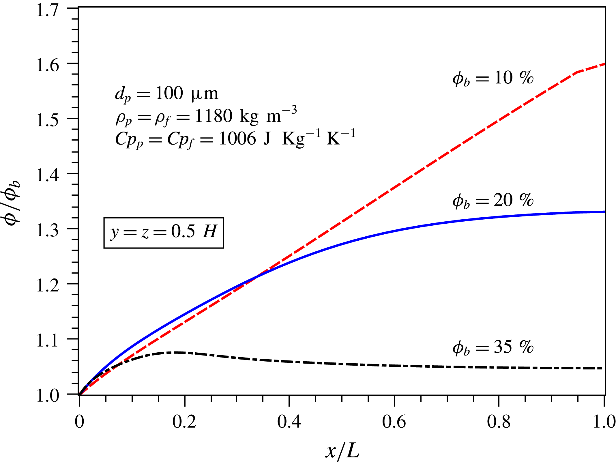
values the particle concentration at the centreline of the channel is observed to stabilize more rapidly towards steady values, as illustrated in figure 15.
Normalized particle volume fraction along the channel’s centreline at the steady state for three different
 $\unicode[STIX]{x1D719}_{bulk}$
values. The initially applied simulation data are:
 $k_{p}/k_{f}=5$
;
 $n=1$
;
 $C_{1}=2.3$
;
 $C_{2}=50$
K;
 $T_{c}=180$
K;
 $d_{p}=100~\unicode[STIX]{x03BC}\text{m}$
;
 ${\unicode[STIX]{x1D702}_{f}}_{i}=8\times 10^{-7}~\text{m}^{2}~\text{s}^{-1}$
;
 ${T_{f}}_{i}=293$
K;
 $\unicode[STIX]{x1D6FD}_{0}=3\times 10^{-4}~\text{K}^{-1}$
;
 $\unicode[STIX]{x1D70C}_{f}=\unicode[STIX]{x1D70C}_{p}=1180~\text{Kg}~\text{m}^{-3}$
;
 $C_{p_{f}}=C_{p_{p}}\approx 1~\text{KJ}~\text{Kg}^{-1}~\text{K}^{-1}$
.

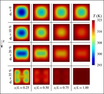
Snapshots of the local temperature at four different cross-section locations along the flow direction at steady state for different initial
 $\unicode[STIX]{x1D719}_{b}$
values. The initially applied simulation data are:
 $k_{p}/k_{f}=5$
;
 $n=1$
;
 $C_{1}=2.3$
;
 $C_{2}=50$
K;
 $T_{c}=180$
K;
 $d_{p}=100~\unicode[STIX]{x03BC}\text{m}$
;
 ${\unicode[STIX]{x1D702}_{f}}_{i}=8\times 10^{-7}~\text{m}^{2}~\text{s}^{-1}$
;
 ${T_{f}}_{i}=293$
K;
 $\unicode[STIX]{x1D6FD}_{0}=3\times 10^{-4}~\text{K}^{-1}$
;
 $\unicode[STIX]{x1D70C}_{f}=\unicode[STIX]{x1D70C}_{p}=1180~\text{Kg}~\text{m}^{-3}$
;
 $C_{p_{f}}=C_{p_{p}}\approx 1~\text{KJ}~\text{Kg}^{-1}~\text{K}^{-1}$
.

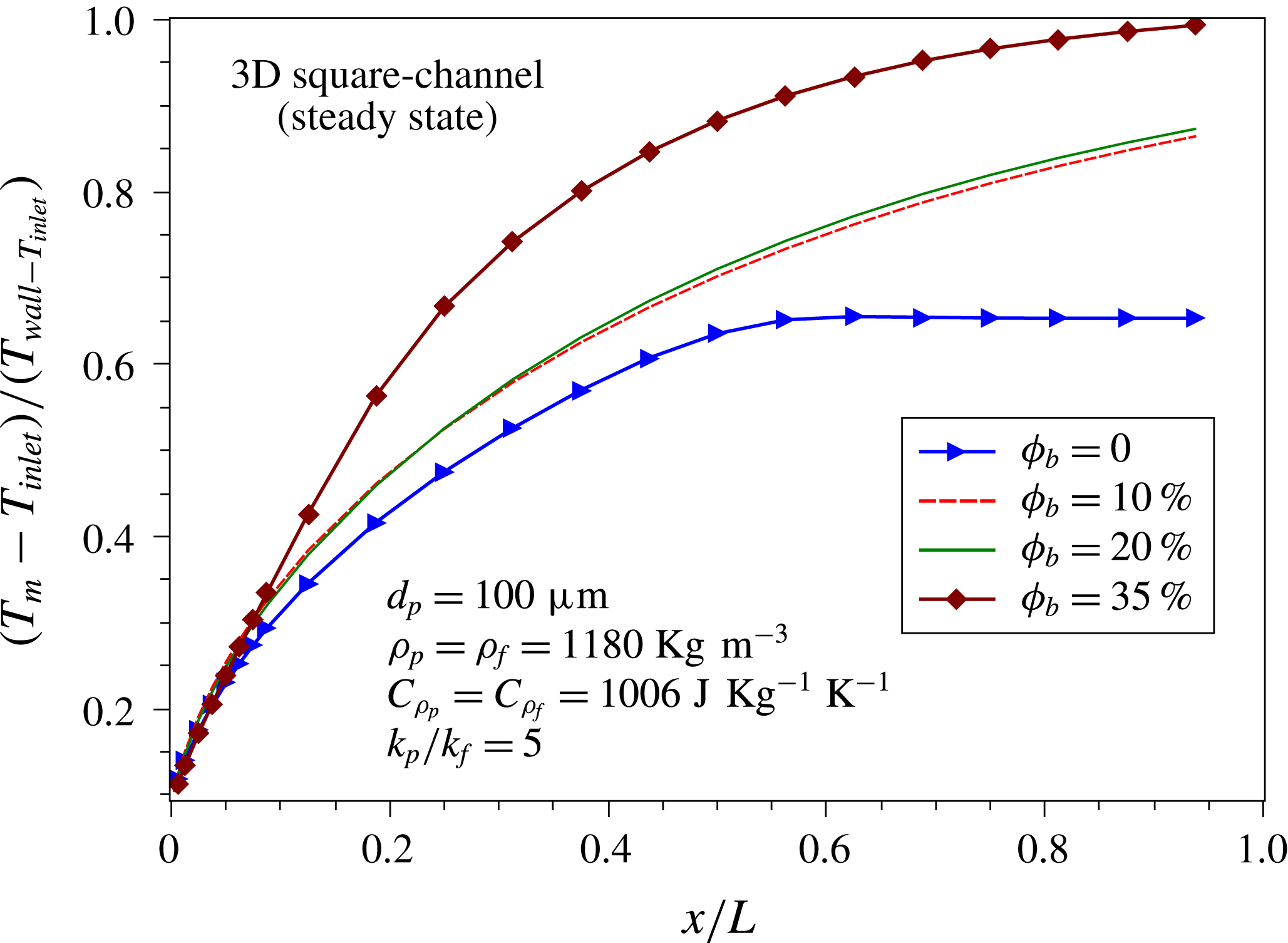
Figure 16 shows snapshots of the local temperature
 $T$
at four different cross-section locations along the flow direction at the steady state. It can be seen that the local temperature values increase, being more uniform, with the increase in the initial bulk volume fraction values. Moreover, at
 $\unicode[STIX]{x1D719}_{b}=35\,\%$
at
 $x/L\leqslant 0.5$
higher
 $T$
values are observed around the centre of the cross-section compared to cases at lower initial
 $\unicode[STIX]{x1D719}_{b}$
values. This can be better explained by looking to the mass-flow-averaged dimensionless temperature values across the channel’s length which are presented in figure 17.
Mass-flow-averaged dimensionless temperature in cross-section along the channel’s length at the steady state for several initial
 $\unicode[STIX]{x1D719}_{b}$
values. The initially applied simulation data are:
 $k_{p}/k_{f}=5$
;
 $n=1$
;
 $C_{1}=2.3$
;
 $C_{2}=50$
K;
 $T_{c}=180$
K;
 $d_{p}=100~\unicode[STIX]{x03BC}\text{m}$
;
 ${\unicode[STIX]{x1D702}_{f}}_{i}=8\times 10^{-7}~\text{m}^{2}~\text{s}^{-1}$
;
 ${T_{f}}_{i}=293$
K;
 $\unicode[STIX]{x1D6FD}_{0}=3\times 10^{-4}~\text{K}^{-1}$
;
 $\unicode[STIX]{x1D70C}_{f}=\unicode[STIX]{x1D70C}_{p}=1180~\text{Kg}~\text{m}^{-3}$
;
 $C_{p_{f}}=C_{p_{p}}\approx 1~\text{KJ}~\text{Kg}^{-1}~\text{K}^{-1}$
.

5 Conclusion and perspectives
CFD modelling and simulation are developed, generalized and validated for conjugate heat transfer and shear-induced migration in dense non-colloidal laminar suspension flows. The suspension effective heat transfer affected by the local shear rate, the phenomenon of shear-induced particle migration, the buoyancy effects and the thermal Péclet number at the particle scale are all considered in the present constitutive three-dimensional Eulerian CFD modelling. Moreover, the influence of the temperature, the shear rate and the particle volume fraction on the suspension effective viscosity, on the suspension effective thermal properties and on the fluid density are also addressed.
The present modelling is validated by simulating and comparing the present numerical results to the experimental ones obtained recently by Metzger et al. (Reference Metzger, Rahli and Yin2013) for a suspension heated and sheared in a Couette cylindrical cell. Then the present CFD model is applied to study heat transfer enhancement by applying dense non-colloidal suspension flow in a square cross-section long channel with
 $D_{h}=5$
mm hydraulic diameter and
 $L/D_{h}=800$
at an effective
 $Re=10$
. A suspension overall heat enhancement factor (
 $\text{STEF}$
), based on the averaged local suspension Nusselt number and local pressure drop, is developed and introduced. Compared to
 $\text{STEF}=1$
for pure fluid cases at
 $\unicode[STIX]{x1D719}_{b}=0\,\%$
,
 $\text{STEF}>1$
values are observed for suspensions at
 $\unicode[STIX]{x1D719}_{b}=10\,\%$
; 20 %; 35 % illustrating heat transfer enhancement in channels by applying non-colloidal suspensions of monodispersed rigid spheres at two different conductivity ratios
 $k_{p}/k_{f}=0.2$
; 5 (for particles of
 $100~\unicode[STIX]{x03BC}\text{m}$
in diameter).
The present contribution constitutes first attempts toward an emerging field of heat transfer applications by using dense suspension flows. Both experimental and numerical investigations will be conducted in the future in order to characterize and quantify well the influence of the suspension flow properties on enhancing heat transfer in different geometrical configurations. This will be crucial for predicting and designing innovative compact heat exchangers for different applications.
Acknowledgement
The author appreciates and thanks Professor B. Metzger for his useful information provided about the experimental work published in Metzger et al. (Reference Metzger, Rahli and Yin2013), and for his useful scientific discussions.