





Introduction
The size of an individual plate of ice—the floe scale—is foundational to sea ice dynamics in the marginal ice zone (MIZ). The relationship between the floe scale and the spatial scales of atmospheric and oceanic motion is important for understanding coupled interactions, as stresses from the atmosphere and ocean are integrated across the surface of the floe (Brenner and others, Reference Brenner2023; Gupta and others, Reference Gupta, Gürcan and Thompson2024; Kim and others, Reference Kim, Manucharyan and Wilhelmus2025). The spacing between floes and the range of floe sizes in an area, characterized by the sea ice concentration (SIC) and the floe size distribution (FSD), respectively, strongly affect air-ocean fluxes, lateral melt rates, wave-ice interactions and floe-floe interactions (McNutt and Overland, Reference McNutt and Overland2003; Loose and others, Reference Loose, McGillis, Perovich, Zappa and Schlosser2014; Roach and others, Reference Roach, Horvat, Dean and Bitz2018; Wenta and Herman, Reference Wenta and Herman2018; Herman, Reference Herman2022; Horvat, Reference Horvat2022; Manucharyan and others, Reference Manucharyan, Lopez-Acosta and Wilhelmus2022; Brenner and Horvat, Reference Brenner and Horvat2024). Thus, joint observations of floe shapes and motion are needed to characterize MIZ sea ice dynamics.
Spatial and temporal variability in ice motion is directly related to the FSD and SIC (Overland and others, Reference Overland, Walter, Curtin and Turet1995; Dumont, Reference Dumont2022; Herman, Reference Herman2022). The FSD is constantly evolving as floes either become larger due to pieces of ice interlocking, rafting, ridging and fusing, or smaller due to fracture and melt (Zhang and others, Reference Zhang, Schweiger, Steele and Stern2015; Horvat and others, Reference Horvat, Tziperman and Campin2016; Bateson and others, Reference Bateson, Feltham, Schröder, Hosekova, Ridley and Aksenov2020; Roach and others, Reference Roach, Smith, Herman and Ringeisen2024). The tight coupling between the seasonally evolving FSD, mesoscale and submesoscale ocean currents, waves and wind stress in the MIZ results in complex sea ice motion patterns with low spatial correlation (meters to kilometers) and short temporal scales (hours to days) (Thorndike and Colony, Reference Thorndike and Colony1982; Hakkinen, Reference Hakkinen1987; Johannessen and others, Reference Johannessen1987a, Reference Johannessen, Johannessen, Svendsen, Shuchman, Campbell and Josberger1987b; Feltham, Reference Feltham2005; Cole and others, Reference Cole2017; Watkins and others, Reference Watkins, Bliss, Hutchings and Wilhelmus2023).
The dynamical complexity of the MIZ poses a key challenge for sea ice observation systems (Gerland and others, Reference Gerland2019; Webster and others, Reference Webster, Rigor and Wright2022a; Sandven and others, Reference Sandven2023). The physical processes that can be resolved are constrained by the spatial resolution and acquisition frequency of observations, as well as whether the system is designed in a Lagrangian or Eulerian framework. SIC, extent, age and motion at large scales have long been routinely available through operational remote sensing products, while satellites capable of sea ice thickness estimates are more recent (Sandven and others, Reference Sandven2023). Few products are capable of resolving sea ice properties at small scales (Müller and others, Reference Müller, Batrak, Dinessen, Grote and Wang2023), and observations of processes at the floe scale are especially sparse. Algorithms for analysis of floe-scale motion have been proposed (Lopez-Acosta and others, Reference Lopez-Acosta, Schodlok and Wilhelmus2019; Wang and others, Reference Wang, König and Oppelt2021); however, with the exception of prior work with the Ice Floe Tracker (IFT) (Lopez-Acosta, Reference Lopez-Acosta2021; Manucharyan and others, Reference Manucharyan, Lopez-Acosta and Wilhelmus2022), no existing data products provide floe shapes and motion simultaneously.
On the one hand, buoys track the motion of individual ice floes with high precision. At scales greater than 100 km, operational buoy deployments through the International Arctic Buoy Program (IABP, Rigor and others (Reference Rigor, Clemente-Colon and Hudson2008)) provide long-term coverage of the sea ice cover. Due to the difficulty and expense of deployment, however, this data is spatially and temporally sparse, particularly in the MIZ (Gerland and others, Reference Gerland2019; Brunette and others, Reference Brunette, Tremblay and Newton2022). In addition, buoy-derived measurements are limited to point-wise acquisitions, which must be collated with other sensors to estimate sea ice properties. For example, the spatiotemporal scale dependence in sea ice motion and deformation is obtained using measurements from buoy arrays (Hutchings and others, Reference Hutchings, Roberts, Geiger and Richter-Menge2011; Itkin and others, Reference Itkin2017).
On the other hand, remote sensing observations from satellites and aircraft enable observation of sea ice properties across large spatial regions. Ice motion is computed from satellite imagery by cross-correlating pixel intensity between consecutive image pairs (Ninnis and others, Reference Ninnis, Emery and Collins1986; Kwok and others, Reference Kwok, Schweiger, Rothrock, Pang and Kottmeier1998). The produced motion vectors represent an area-average within the spatial window used by the correlation algorithm. In the pack ice, where spatial correlation is high, the sea ice moves coherently and displacement estimates have high confidence; however, the same spatial window in the MIZ may include thousands of jostling floes, resulting in higher uncertainty (Sumata and others, Reference Sumata2014; Gui and others, Reference Gui, Lei, Pang, Hutchings, Zuo and Zhai2020). Moreover, many products are only available seasonally, with few products providing estimates of motion during the summer melt season due to the presence of liquid water at the snow-and-ice surface affecting the quality of the images and the ability to distinguish between surface melt water and leads (Lavergne and others, Reference Lavergne, Eastwood, Teffah, Schyberg and Breivik2010; Girard-Ardhuin and Ezraty, Reference Girard-Ardhuin and Ezraty2012). Thus, the representativeness, availability and uncertainty of remote sensing-derived ice motion vectors vary spatially and temporally, and are degraded in the MIZ.
In contrast to sea ice motion, the FSD is not routinely measured, though standard operational ice charts do include information on predominant floe size categories (Dedrick and others, Reference Dedrick, Partington, Van Woert, Bertoia and Benner2001; Afanasyeva and others, Reference Afanasyeva2019). Historically, most studies of the FSD have been based on small numbers of images (Stern and others, Reference Stern, Schweiger, Zhang and Steele2018b) and processed image data was only available upon request from the authors, though recent studies have greatly expanded access to processed sea ice imagery (Buckley and others, Reference Buckley, Cañuelas, Timmermans and Wilhelmus2024).
Traditional methods and image types used to characterize the FSD vary (Paget and others, Reference Paget, Worby and Michael2001; Toyota and others, Reference Toyota, Takatsuji and Nakayama2006; Hwang, Reference Hwang2013). Most commonly, the FSD is characterized via a power law with the form
 \begin{equation}
p(x) = cx^{-\alpha}
\end{equation}
where  $x$ is a measure of floe size,
 $c$ is a normalization constant and the parameter
 $\alpha$ is the slope of the power law distribution on a log-log scale. This representation assumes an approximately linear FSD probability density function (PDF) in log-log space (Rothrock and Thorndike, Reference Rothrock and Thorndike1984). While this form is convenient given its direct application in models, the power law in Eq. (1) is an empirical, not theoretical result (Herman, Reference Herman2010) and distinct mechanisms governing the evolution of the FSD may lead to other forms of the FSD PDF. Indeed, FSD characteristics vary substantially across studies (Stern and others, Reference Stern, Schweiger, Zhang and Steele2018b), often showing a clear departure from Eq. 1. Differences in methodology across FSD studies pose a challenge for developing a unified theory for FSD evolution. For example, theoretical and model-based analyses of floe breakup through wave action suggest a log-normal FSD (Mokus and Montiel, Reference Mokus and Montiel2022; Montiel and Mokus, Reference Montiel and Mokus2022), while Toyota and others (Reference Toyota, Haas and Tamura2011) found that observed FSDs had different power law slope parameters in different size regimes.
The lack of consistent, joint observations of FSD and ice motion, over a representative range of sea ice conditions, also poses a challenge for sea ice model development and validation. The inclusion of FSD parameterizations in continuum models (e.g., Hunke and Dukowicz (Reference Hunke and Dukowicz1997)) is seen as a potential path forward for better simulation of small-scale thermodynamic and dynamic sea ice processes and wave-ice interactions (Horvat and Tziperman, Reference Horvat and Tziperman2015; Zhang and others, Reference Zhang, Schweiger, Steele and Stern2015; Roach and others, Reference Roach, Horvat, Dean and Bitz2018; Bateson and others, Reference Bateson, Feltham, Schröder, Hosekova, Ridley and Aksenov2020). Such parameterizations provide links between the statistics of the FSD and other sea ice processes, rather than explicitly representing ice floes. Alternatively, discrete element method (DEM) models include the effects of the FSD on ice motion either explicitly (disks, polygons, e.g., Damsgaard and others, Reference Damsgaard, Adcroft and Sergienko2018; Manucharyan and Montemuro, Reference Manucharyan and Montemuro2022; Gupta and others, Reference Gupta, Gürcan and Thompson2024) or implicitly through bonded particles (Aström and Polojärvi, Reference Åström and Polojärvi2024). These models have proven especially valuable for process studies, for example, examination of coupled interaction between mesoscale ocean turbulence and sea ice melt processes (Gupta and Thompson, Reference Gupta and Thompson2022) and the development of turbulence under sea ice (Brenner and others, Reference Brenner2023). Excepting dedicated experiments where multiple observation sources are merged (e.g., Uttal and others, Reference Uttal2002; Hwang and others, Reference Hwang2017; Rabe and others, Reference Rabe2024), modelers must rely on disparate case studies for the FSD (Stern and others, Reference Stern, Schweiger, Zhang and Steele2018b) and use complementary datasets to validate motion (Tsarau and others, Reference Tsarau, Lu, Lubbad, Løset and Zhang2024).
In this study, we present and analyze novel observations of sea ice properties and motion at the floe scale derived from optical satellite imagery. We first provide details of the source data, the floe detection algorithm and the floe tracking routine. Then, we investigate the statistical properties and seasonal evolution of sea ice floe properties, the FSD, floe-scale motion and links between motion and floe properties. We compare the floe-scale motion estimates to large-scale ice motion vectors and analyze the drift anomaly distribution. Finally, we consider the spatial variation of velocity through analysis of the length scale dependence of sea ice deformation. Our focus is on the Fram Strait and East Greenland seasonal ice zone due to its importance as a connection between the Arctic and the world oceans (Smedsrud and others, Reference Smedsrud, Halvorsen, Stroeve, Zhang and Kloster2017; Sumata and others, Reference Sumata, De Steur, Gerland, Divine and Pavlova2022), as it is the main passage of sea ice export from the Arctic Ocean. In addition, the presence of sharp gradients in the ocean currents and distinct mesoscale features affecting the ice dynamics (Manley, Reference Manley1987; Kozlov and Atadzhanova, Reference Kozlov and Atadzhanova2021; Morozov and Kozlov, Reference Morozov and Kozlov2023; Watkins and others, Reference Watkins, Bliss, Hutchings and Wilhelmus2023) makes it an ideal testbed for measuring complex, small-scale sea ice dynamics. Our observations aim to fill a major observational data gap for sea ice dynamics in the spring-to-summer MIZ.
Data
Satellite imagery
We acquired daily 250-m resolution true color (bands 1–3–4) and false color (bands 7–2–1) mosaic imagery from the Moderate Resolution Imaging Spectroradiometer (MODIS) instruments via the NASA Worldview Snapshots utility. Two images are used each day, corresponding to the daytime overpasses of the Aqua and Terra satellites. Overpass times for the two satellites are generally between 20 and 90 minutes apart. Data are provided on a North Polar Stereographic grid. As imagery is only labeled with the date, we use the Satellite Overpass Identification Tool (Hatcher and others, Reference Hatcher, Ahmed, Kim and Wilhelmus2022) to identify the precise overpass time for each image for use in ice motion calculations. The study region covers the area northeast of Greenland from the Fram Strait in the north to Scoresby Sound in the south (Fig. 1, green box). We focused on the spring and summer months (April 1 to September 15) to ensure consistent illumination, and cover years 2003–20. Sea ice in the region has a large seasonal cycle and significant year-to-year variability. Blue and pink lines in Fig. 1 mark the April and September mean sea ice extent for each year from the National Snow and Ice Data Center (NSIDC) Sea Ice Index (Fetterer and others, Reference Fetterer, Knowles, Meier, Savoie and Windnagel2017). The end-of-season ice extent exhibits greater year-to-year variability than winter extent.
Map of the study region (green box) and extent of image details for subsequent figures (orange and purple boxes). Blue lines show the mean April sea ice extent for each year 2003–20, while pink lines show the September mean.

Figure 1 Long description
A map depicting the study region northeast of Greenland, marked by a green box. Blue lines indicate the mean April sea ice extent, while pink lines show the September mean. An orange box outlines the area and a purple box. The map includes latitude and longitude lines, with the region extending from approximately 50 degrees west to 20 degrees west and from 65 degrees north to 80 degrees north. The legend identifies the colors and their corresponding meanings.
Gridded sea ice data products
We use the NSIDC Daily Ice Motion Vectors data product of time-average sea ice drift at moderate-to-large scales (Tschudi and others, Reference Tschudi, Meier and Stewart2020). This product merges ice motion estimates from passive microwave imagery, buoys and from reanalysis wind data. The motion vectors are provided on a 25-km grid at daily resolution. Note, however, that the effective resolution is generally coarser than this, as the source satellite motion resolution ranges from 37.5 to 75 km (Tschudi and others, Reference Tschudi, Meier and Stewart2020). We use SIC from the NOAA/NSIDC Climate Data Record (CDR) of SIC to characterize the SIC of the region around each floe. This product combines SIC estimates from the NASA Team and NASA Bootstrap algorithms by choosing the maximum concentration from each source (Meier and others, Reference Meier, Fetterer, Windnagel and Stewart2021, Reference Meier, Stewart, Windnagel and Fetterer2022). While higher resolution SIC estimates are available during some years and seasons (e.g., Spreen and others (Reference Spreen, Kaleschke and Heygster2008)), the primary advantage of using the NOAA/NSIDC CDR is consistent, daily time-resolution data across all years and months of the study period, with equivalent accuracy to other satellite-based SIC estimates compared to in situ observations (Kern and others, Reference Kern2019). Due to its design as the maximum of two algorithms, it tends to have a positive bias. It is important to note that the uncertainty in passive microwave estimates of SIC increases during the melt season and toward the ice edge. We estimate local SIC at floe positions via nearest-neighbor interpolation. We calculate the distance to the ice edge by finding the minimum distance between each floe and the set of pixels with zero concentration in the SIC CDR. Similarly, we estimate the distance to the coast by searching for the minimum distance to the grid cells in the NSIDC data products flagged as land. We compute the regional sea ice extent as the area of grid cells in the SIC CDR with SIC  $\geq$ 15%. In addition, we compute the MIZ ice extent, defined as the sea ice extent for grid cells with SIC between 15 and 85%, and the MIZ ice fraction, defined as the MIZ ice extent divided by the regional sea ice extent.
Methods
Sea ice segmentation and tracking
We obtain measurements of floe-scale sea ice motion derived from moderate resolution optical satellite imagery using the IFT algorithm (Lopez-Acosta and others, Reference Lopez-Acosta, Schodlok and Wilhelmus2019). The dataset consists of segmented satellite imagery, floe shape statistics and derived floe trajectories. We first describe the source data, algorithm and post-processing routines, then summarize the contents of the dataset. The full dataset is available from the Brown Digital Repository at https://doi.org/10.26300/ydtf-e778.
Ice Floe Tracker algorithm
The IFT algorithm identifies and tracks ice floe shapes in an image sequence to reconstruct their motion trajectories. The algorithm consists of five subroutines: (1) data acquisition, (2) pre-processing, (3) segmentation, (4) tracking and (5) post-processing (Fig. 2). Steps 2–4 are described in detail in Lopez-Acosta and others (Reference Lopez-Acosta, Schodlok and Wilhelmus2019) and Lopez-Acosta (Reference Lopez-Acosta2021) and are briefly summarized here, while the post-processing routine is introduced here.
Overview of the Ice Floe Tracker processing pipeline.

Figure 2 Long description
A flowchart illustrating the Ice Floe Tracker processing pipeline. The first stage is Data Acquisition, which includes MODIS true color (1-4-3), MODIS false color (7-2-1) and OpenStreetMap land mask. The second stage is Pre-processing, involving land mask dilation, nonlinear diffusion, adaptive histogram equalization and sharpening. The third stage is Segmentation, which consists of image binarization, watershed transformation and morphological cleanup. The fourth stage is Tracking, which includes checking travel distance, geometric comparisons and tie-breaking. The final stage is Post-processing, involving area bias correction, trajectory outlier flagging, logistic regression filter and data formatting and archiving. Arrows indicate the flow from one stage to the next.
Pre-processing of MODIS true and false color images comprises de-noising via anisotropic diffusion filtering, contrast adjustment by adaptive histogram equalization and unsharp masking, and noise removal by morphological reconstruction. These procedures produce a sharpened grayscale image (Fig. 3a–f). Next, we apply a combination of morphological operations and  $k$-means clustering to segment the pre-processed image into ice and water regions. Watershed segmentation is used to separate ice regions into individual floes. In this method, images are analyzed as topographic maps by identifying markers using the local maxima of the distance to water pixels, then producing closed contours by so-called flooding of the image. The method is applied both to the binary
 $k$-means result and to the sharpened grayscale image. The intersection of the two watershed boundaries is used to divide the
 $k$-means result into individual floes.
Top: (a) True color, (b) false color and (c) processed images for 24 April 2013 from the Aqua satellite. In the processed image, masked regions (including the dilated land mask and the cloud mask) are black. Candidate segments are labeled as either floes (orange) or non-floes (light blue); non-floes are discarded in the final product. Middle: As in (a)–(c) for the Aqua image for 1 May 2014. Bottom: Details of true color images from (g) 24 April 2013 and (h) 1 May 2014 with overlaid IFT segmentation results, with objects labeled as floes marked in orange and discarded objects in light blue. Manually identified floe boundary for the true positive floes is shown in dark blue. Bounds for the images are shown in panels (c) and (f), respectively. Panel (i) shows the area of manually labeled well-segmented objects versus IFT results for the 24 April 2013 and 1 May 2014 initially (gold) and after area adjustment (blue). Objects with poor correspondence to manual floe labels are marked in gray. The one-to-one line is shown in black. Image locations for panels (a) through (f) are shown in Figure 1.

Figure 3 Long description
The image A shows the true color satellite image from 24 April 2013 with axes labeled X (times 10 superscript 6 m) and Y (times 10 superscript 6 m). The image B shows the false color satellite image from the same date with the same axes. The image C shows the processed image from 24 April 2013, highlighting non-floes, floes and masked regions. The image D shows the true color satellite image from 01 May 2014 with similar axes. The image E shows the false color satellite image from the same date. The image F shows the processed image from 01 May 2014, also highlighting non-floes, floes and masked regions. The image G shows the segmentation results for 24 April 2013, with floes marked in orange and non-floes in light blue. The image H shows similar segmentation results for 01 May 2014. The image I is a graph showing area adjustment, with axes labeled IFT Area (kilometer squared) and Manual Area (kilometer squared), displaying initial and adjusted data points along a one-to-one line.
Finally, we label the connected components of the segmented image and extract shape properties (e.g., area, perimeter, centroid, average reflectance) from potential floes. The error in discrete representations of shapes tends to increase as the size decreases. In addition, prior studies have found few floes larger than 30-50 km (Stern and others, Reference Stern, Schweiger, Stark, Zhang, Steele and Hwang2018a, Reference Stern, Schweiger, Zhang and Steele2018b). Hence, only candidate floes with sizes of at least 300 pixels and at most 90,000 pixels are retained, equivalent to 18.75-5,625 km $^2$ in area, corresponding to length scales of 4.3-75 km. We estimate local SIC at floe positions via nearest-neighbor interpolation. We calculate the distance to the ice edge by finding the minimum distance between each floe and the set of pixels with zero concentration in the SIC CDR. Similarly, we estimate the distance to the coast by searching for the minimum distance to the grid cells flagged as land in the CDR.
The floe tracking component links floe shapes across image pairs. For each floe, candidate matches in subsequent images are selected by first filtering by travel distance and floe area. Potential floe matches are rotated until the area difference is minimized. If the area difference is sufficiently small after rotation,  $\psi - s$ curves (Kwok and others, Reference Kwok, Curlander, McConnell and Pang1990) are calculated for each floe. These curves summarize the tangent angle,
 $\psi$, and arc length,
 $s$, of each floe. If the
 $\psi - s$ correlation is higher than 0.7, the floes are linked. Whether a floe can be tracked depends mainly on cloud cover, whether the floe remains intact, and on the algorithm accuracy in identifying the floe shape. As an illustration, a subset of detected floes is shown in Fig. 4, highlighting those which were successfully tracked for at least three of the four depicted days. The tracker allows time gaps of at most three days, hence a floe missed in one observation may still be successfully tracked in subsequent images. Given that up to two position estimates are available for each day (corresponding to the Aqua and Terra overpass times), daily rotation rates are calculated using the mean daily rotation across the two satellites when both are available; otherwise, we use rotation from a single satellite. Rotation rates are then normalized to radians per day.
Floe shapes and trajectories for a set of floes tracked in Aqua imagery from 27 to 30 April 2014. To reduce visual clutter, floe trajectories are only shown for floes that appear in at least three of the four images. Satellite overpass time is marked in the title. Image location is shown in Figure 1. Markers show the positions of the floe centroid between 27 April 2014 and the image time.

Figure 4 Long description
The image consists of four satellite images labeled a, b, c and d, showing floe trajectories over four days from 27 to 30 April 2014. Each image is marked with a date and time: a) 27 April 2014 at 12:38, b) 28 April 2014 at 11:43, c) 29 April 2014 at 12:26 and d) 30 April 2014 at 11:31. The x-axis and y-axis are labeled in kilometers, ranging from negative 100 to 100. Various colored lines and markers indicate the positions and paths of floes over the days. The background shows a detailed view of ice floes in a polar region, with each image capturing changes in floe positions and movements over time. The images illustrate the dynamic nature of the ice floes, with distinct paths and positions marked for each day, highlighting the movement and rotation of the floes across the observed period.
Post-processing
The IFT image processing returns significantly more candidate ice floe shapes than it is able to track. These candidate ice floe shapes contain both untracked floes and false positives, such as ice filaments and clouds. In Lopez-Acosta and others (Reference Lopez-Acosta, Schodlok and Wilhelmus2019), the floe tracking served as a filter to remove objects such as bright clouds that had been mislabeled as sea ice. In order to leverage shapes from untracked floes for FSD analysis, we developed a post-processing routine to identify which of the untracked objects are likely to be ice floes. The light blue regions in Fig. 3c, f and h are examples of rejected shapes. We implemented a logistic regression classifier to assign each object a probability of being an ice floe. Training and testing the classifier required identifying a set of true and false positives. True positives were selected from the set of tracked floes such that (a) trajectory mean drift speeds are less than 1 m/s and (b) trajectory maximum drift speed is larger than 0.05 m/s, i.e., moving at least two pixels per day. False positives were identified using circularity and solidity thresholds. Circularity is defined as
 \begin{equation}
C = \frac{4\pi A}{P^2}
\end{equation}
where  $A$ is the floe area and
 $P$ is the floe perimeter, such that a perfect circle has
 $C=1$, while solidity
 $S$ is the ratio of the area of the shape to the area of the smallest enclosing convex polygon. Objects with
 $S \leq 0.4$ or
 $C \leq 0.2$ were labeled as false positives.
A final source of false positives comes from estimating the local SIC. We applied nearest neighbor interpolation to the NSIDC SIC data to find the SIC in the nearest grid cell to the IFT floe positions. Objects with SIC=0 were classified as false positives. Prior to model fitting, we stratified the sample by year and month, randomly selecting up to 1,000 true and false positives from each subgroup. The randomly sampled data were split into training and testing portions, then trained using 10-fold cross-validation. Model fitting was carried out using the Python Scikit-Learn machine learning library (Pedregosa and others, Reference Pedregosa2011). The algorithm performs well, with a precision score of 0.92 and a recall score of 0.9.
Comparison of the IFT floe shapes with manually annotated imagery shows that the methods used to separate neighboring floes produce a systematic underestimate of floe area (Fig. 3g–i). The detected floe boundary is approximately a constant number of pixels inside the true floe boundary. As a result, the relative error in area is greater for small floes than for large floes. For a floe with detected segment area  $A_0$, we implement a simple bias correction factor by adding a fixed offset
 $\delta L$ to the floe length scale
 $L_0 = \sqrt{A_0}$, such that the corrected area
 $A$ is given by
 \begin{equation}
A(L_0) = (L_0 + \delta L)^2
\end{equation}
and the corrected length scale is  $L = L_0 + \delta L$.
To find an optimal value for  $\delta L$, we manually labeled
 $n=1,071$ true floe boundaries for IFT candidate floes across five images. Pairs of true floes and candidate floes were divided into test and training sets, with 2/3 going into the training set. We then identified quality candidate objects using the area fraction of the overlap. Setting thresholds of overlap area to at least 90% of the candidate floe area and 40% of the ground truth floe area removed under-segmented objects well, yielding
 $n=440$ well-segmented floe pairs. Minimizing the mean absolute error in area using the well-segmented pairs yields an optimal correction factor of
 $\delta L = 8$ pixels, with a mean absolute error of 10.6 km
 $^2$ (median 4.9 km
 $^2$) for the well-segmented pairs. Finally, using all test-set floe pairs marked as clean by the logistic regression, absolute error has a long tail with a few large outliers, resulting in mean absolute error of 79.6 km
 $^2$ (median 12.0 km
 $^2$).
IFT data summary
Detected sea ice floes cover the region of the Greenland Sea where sea ice is typically found (Fig. 5a and b). The lowest detection frequency is near the edge of the seasonal maximum ice extent, and the highest floe concentrations are seen nearer to the center of the seasonally sea ice-covered region. The highest concentration of detected floes is in the southern portion of the study area. Trajectories reflect the southward, nonlinear motion of sea ice (Fig. 5c). The raw segmented imagery contains approximately  $10^5$ objects per year, with about half as many passing the quality control algorithm (blue and orange lines in Fig. 5d). The number of detected floes passing quality control shows a distinct climatology (Fig. 5e, Fig. S1) with many more floes available early in the year. The number peaks in April and has a secondary peak in June, related to landfast ice breakup. By July, ice extent is much lower and few images have more than 100 floes. Detecting rotation and drift requires pairs of images and successful floe matching, resulting in the number of rotation estimates being on the order of
 $10^3$ per year; since an individual trajectory can have multiple rotation measurements, the number of individual tracked objects is slightly reduced (pink and green lines in Fig. 5d). Most trajectories are between two and ten days long, and the number of trajectories has strong inter-annual variability (Fig. 5f).
Top: spatial histograms of (a) all available sea ice floe shapes and (b) tracked floes. Floe centroids were binned into 25 km by 25 km grid cells for enumeration. (c) Ice floe trajectories for floes tracked for a period of at least 7 days. Bottom: (d) Number of floes per year in the raw Ice Floe Tracker output (blue) and after postprocessing (orange). The number of tracked floes is shown in green and the number of rotation rate estimates is in pink. (e) Distribution of the number of floes per image as a function of day of year. Counts were smoothed using a 15-day centered median. Floe counts separated into untracked and tracked categories without smoothing are shown in Supplemental Figure S1. (f) Histograms of trajectory lengths in days for each year.

Figure 5 Long description
The image contains six graphs related to sea ice floe data. The first graph (a) shows a spatial histogram of all available sea ice floe shapes, with counts ranging from 0 to 1800. The second graph (b) displays tracked floes with similar count ranges. The third graph (c) illustrates ice floe trajectories tracked for at least seven days, showing various paths. The fourth graph (d) presents the number of floes per year from 2005 to 2020, with lines for raw, clean, tracked and rotation data. The fifth graph (e) shows the distribution of the number of floes per image as a function of the day of the year, with counts smoothed using a 15-day centered median. The sixth graph (f) depicts histograms of trajectory lengths in days for each year, with data from 2003, 2006, 2009, 2012, 2015 and 2018.
Floe size distribution
The sea ice FSD has been shown to be approximately linear in log-log space for at least some range of floe sizes. As such, it has frequently been summarized through fitting a power law of the form in Eq. 1 (Rothrock and Thorndike, Reference Rothrock and Thorndike1984; Stern and others, Reference Stern, Schweiger, Zhang and Steele2018b). A common approach to estimating power law fits of this form from empirical data is to apply a log-transform to the data and fit a line using least squares. Due to the effects of sparse but high-impact fluctuations in the tail of the distribution, this method can be inaccurate; furthermore, the least squares method does not test whether a power law is appropriate (Goldstein and others, Reference Goldstein, Morris and Yen2004; Bauke, Reference Bauke2007; Clauset and others, Reference Clauset, Shalizi and Newman2009). Other distributions, such as a truncated power law or lognormal distribution, may fit the data better, while still explaining the approximately linear scaling seen in the log-log plots (e.g., Burroughs and Tebbens, Reference Burroughs and Tebbens2001; Toyota and others, Reference Toyota, Takatsuji and Nakayama2006; Lu and others, Reference Lu, Li, Zhang and Dong2008; Herman, Reference Herman2010; Montiel and Mokus, Reference Montiel and Mokus2022). In this study, we follow the approach of Clauset and others (Reference Clauset, Shalizi and Newman2009), as implemented in the Python powerlaw package (Alstott and others, Reference Alstott, Bullmore and Plenz2014). We focus on the power law, truncated power law and lognormal distributions due to their frequent use in the literature. Multiple distributions are referred to as truncated power laws across different studies. Here, we use the form
 \begin{equation}
p(x) = cx^{-\alpha}e^{-\lambda x}
\end{equation}
where  $p(x)$ is the probability of a floe having area
 $x$,
 $c$ is a normalizing constant,
 $\alpha$ is the power law slope parameter and
 $\lambda$ is a parameter controlling the rate of cut-off as
 $x$ grows large. The lognormal distribution is defined using parameters
 $\mu$ and
 $\sigma$ and has the PDF
 \begin{equation}
p(x) = \frac{1}{x\sigma\sqrt{2\pi}}\exp\left(-\frac{(\ln x - \mu)^2}{2\sigma^2}\right).
\end{equation}
Best-fit parameters for each distribution are identified using maximum likelihood.
Since the fitted distributions depend on the minimum value of  $x$, we apply a constant
 $x_{min}$ for the full analysis. The optimal
 $x_{min}$ is determined by a simple numerical experiment (Fig. 6). Using 300 randomly selected images, for each value of
 $x_{min}$ from 1 to 75 km we find the best-fit parameters for each parametric distribution. The Kolmogorov-Smirnov distance
 $D_{KS}$, defined as the supremum of the distance between the data and the best-fit parametric distribution, is used to measure the goodness of fit. The optimal
 $x_{min} = 41$ km
 $^2$ is found by minimizing the ensemble mean
 $D_{KS}$ (dashed line in Fig. 6a–c). The model fit improves rapidly as
 $x_{min}$ increases to 41 km
 $^2$, then degrades past that value. Variation across ensemble members is small compared to the variation with
 $x_{min}$ (Fig. 6a–c).
Ensemble mean (solid line), standard deviation (dark shading) and min-max range (light shading) of  $D_{KS}$ for the best-fit parametric distribution as a function of
 $x_{min}$ for (a) power law, (b) truncated power law and (c) lognormal distributions. Vertical dashed lines mark
 $x_{min}=$41 km
 $^2$. (d) Relative error in power law
 $\alpha$ estimate by subsample size relative to images with greater than 300 floes. The median, 25-75% percentile range, and the 10-90% percentile range are shown as the solid line, dark shading, and light shading, respectively.

Figure 6 Long description
The image contains four graphs labeled a, b, c and d. Graph a shows the KS Statistic for Power Law with the x-axis labeled 'Value of x-min (km squared)' and the y-axis labeled 'KS Statistic'. The graph includes a mean line, standard deviation shading and min-max range shading, with a vertical dashed line at 41 km squared. Graph b displays the KS Statistic for Truncated Power Law with similar axes and features as graph a. Graph c presents the KS Statistic for Lognormal distribution, also with similar axes and features. Graph d illustrates Sampling Error with the x-axis labeled 'Minimum number of floes' and the y-axis labeled 'Relative Error'. It includes a median line, 25-75 percent shading and 10-90 percent shading.
It is important to note that the IFT dataset provides a sample of floes in each image, not a complete enumeration. The identifiable floes are constrained by the characteristics of MODIS data, including its 250 m spatial resolution and frequent cloud cover that obscures many floes in the visible imagery. Even though the post-processing performs well, some false positives remain in the floe library, adding further uncertainty to the estimated FSD. The MODIS images and the bounds of the study domain are sufficiently large such that the maximum observable floe size is not constrained by image dimensions, meaning finite size effects (Stern and others, Reference Stern, Schweiger, Zhang and Steele2018b) have a minimal impact on the tail of the recovered distribution. However, our ability to estimate the FSD in a scene based on a sample of floes depends on the sample size. In the absence of large sets of manually annotated imagery, we simulate the effect of subsampling by computing the relative error in power law  $\alpha$ estimates (Fig. 6d). We randomly selected 100 images with at least 300 floes in each, then repeatedly sampled
 $n$ floes from each image without replacement and recalculated
 $\alpha$. We chose the minimum threshold of floes per image for FSD analysis based on a pragmatic balance between the number of floes available in a typical image by day of year (Fig. 5e) and the estimated sampling uncertainty (Fig. 6d). With
 $n=100$, we have
 $\alpha$ errors within
 $\pm 5\%$ in 80% of cases, while still retaining some late-summer data.
In addition to the image-by-image calculation, we also calculate FSD fits for the data binned by day of year. This estimates a central tendency of the distribution, and enables us to estimate FSD later in the year when the per-image sample size is too low. In addition, it allows us to examine variation within subsets of the data.
We weigh the suitability of the three candidate parametric distributions for describing the observed FSD. The distance between the fitted and empirical distributions was assessed with the K-S statistic  $D_{KS}$. P-values are determined by repeatedly drawing samples from the fitted distribution, calculating the fit to the sampled values, and calculating
 $D_{KS}$. The p-value is then determined by the percentage of the K-S statistics from the resampling procedure that are larger than the
 $D_{KS}$ for the original data.
Sea ice drift
Sea ice motion in the IFT is derived from matched pairs of ice floes across multiple days. Thus, as is the case for other remote sensing-based ice drift estimates, we can only measure net displacement between acquisition times, rather than measuring the instantaneous floe velocity. The mean floe speed during a day is bounded below by the net displacement per day. Ice motion vectors
 \begin{equation}
\mathbf{u}_{IFT} = (u_{IFT}, v_{IFT})
\end{equation}
where  $u_{IFT}$ is the zonal and
 $v_{IFT}$ the meridional component of motion are estimated from the floe centroid time series with reference to the polar stereographic projection. Up to two position estimates are available for each day corresponding to the Aqua and Terra overpass times. The satellite overpass times are typically less than 2 hours away from 12 UTC. We regrid the centroid positions to a fixed-time grid using bilinear interpolation, and estimate the motion using forward differences.
For a portion of the analysis, we consider the velocity variability after removing the effects of the mean flow. With reference to an area and time mean  $\langle \mathbf{u} \rangle_{\chi, \tau}$, where
 $\chi$ is the spatial scale and
 $\tau$ the time scale, the sea ice drift anomaly vector
 \begin{equation}
\mathbf{u'} = \mathbf{u} - \langle \mathbf{u} \rangle_{\chi, \tau}
\end{equation}
can be expressed as an along-track (longitudinal) perturbation  $\mathbf{u'}_L$ and a cross-track (transverse) perturbation
 $\mathbf{u'}_T$ such that
 \begin{equation}
\mathbf{u'} = \mathbf{u'}_L + \mathbf{u'}_T
\end{equation}
with  $\mathbf{u}'_L$ parallel to
 $\langle \mathbf{u} \rangle_{\chi, \tau}$ and
 $\mathbf{u}'_T$ perpendicular to
 $\langle \mathbf{u} \rangle_{\chi, \tau} $(LaCasce, Reference LaCasce, Weiss and Provenzale2008; Gabrielski and others, Reference Gabrielski, Badin and Kaleschke2015). The transverse drift component is often termed the perturbation velocity in the literature.
We use centered-time averages of the NSIDC Ice Motion Vectors product to represent the mean flow. We use the NSIDC product rather than the IFT vectors for the spatiotemporal average because the IFT vector locations are not homogeneous in time or space. The properties of  $\mathbf{u}'$ depend on the choice of the mean flow (Rampal and others, Reference Rampal, Weiss, Marsan and Bourgoin2009). We treat the NSIDC grid size as an implicit spatial scale and consider time windows of
 $\tau=5, 15, $ and
 $31$ days. The symmetry of the resulting drift anomaly distribution is an indicator of whether the mean flow has been removed correctly.
Strain rate estimation
Area-averaged strain rates are calculated using Green’s theorem from sets of point estimates of sea ice velocities along a polygon boundary (e.g., Kwok and others (Reference Kwok, Cunningham and Hibler2003); Hutchings and others (Reference Hutchings, Heil, Steer and Hibler2012); Rampal and others (Reference Rampal2019); Dierking and others (Reference Dierking, Stern and Hutchings2020)). Given a set of  $N$ ice floe positions
 $\mathbf{x}$ and motion estimates
 $\mathbf{u}(\mathbf{x})$, we iterate over all possible triangles formed by subsets of floe positions and retain all triangles with minimum interior angle of 20
 $^\circ$ or greater. This procedure yields millions of polygons; since the number of available polygons is bounded above by a combinatorial function, the number of polygons varies widely per year. Using all possible polygons, as was done in Itkin and others (Reference Itkin2017), results in considerable overlap between polygons in some regions. Due to the large study area, we find that the degree of polygon overlap varies considerably from small to large scales, which may lead to prescribing uneven spatial weight across scales. Small polygons are generally non-overlapping, and large polygons nearly all overlap. To minimize spatial biases from overlapping polygons, we downsample iteratively to find sets of non-overlapping polygons within logarithmically spaced length scale bins. In each image, we randomly choose a starting polygon, then iterate through the list of remaining polygons, keeping a polygon if the intersection with previously chosen polygons has zero area (e.g., Fig. 7). For consideration of spatial scaling, we further downsample by drawing random samples within each length scale bin so that equal numbers of samples within each bin are used.
Detected floe shapes in the Terra image for 24 April 2013 (orange). Triangles formed using selected ice floes as vertices (outlined in black) are used to calculate area-averaged strain rates. Examples of triangles at length scales of (a)  $17.6$ km, (b)
 $28$ km and (c)
 $48.6$ km are shown, with the length scale defined as the square root of the triangle area.

Figure 7 Long description
The image consists of three maps labeled a, b and c, each showing ice floe shapes in orange with triangles outlined in black. Map a shows triangles with a length scale of approximately 17.6 kilometers. Map b displays triangles with a length scale of approximately 28.0 kilometers. Map c features triangles with a length scale of approximately 48.6 kilometers. The x-axis is labeled X times 10 superscript 6 meters and the y-axis is labeled Y times 10 superscript 6 meters. Each map illustrates different spatial arrangements of ice floes and the corresponding triangles used for analysis.
The Green’s theorem approach for strain rate calculation uses the line integral around a region to calculate the area average of the gradient of a quantity. Given drift vectors  $\mathbf{u} = (u, v)$ measured at
 $N$ points
 $\mathbf{x} = (x, y)$ forming the vertices of a polygon, the mean velocity gradients within the polygon are calculated as
 \begin{align}\overline{u}_x & = \frac 1A \oint u \, dy \nonumber\\
& \approx \frac{1}{2A} \sum_{i=1}^N \left[(u_{i+1} + u_i)(y_{i+1} - y_i)\right],\end{align}
where in the summation notation used here, the calculation wraps clockwise around the polygon to the origin. Hence, for the triangles used here,  $x_4 = x_1$. Other ice drift gradients are calculated in a similar fashion (see, e.g.,
Lindsay and Stern (Reference Lindsay and Stern2003); Hutchings and others (Reference Hutchings, Roberts, Geiger and Richter-Menge2018); Bouchat and Tremblay (Reference Bouchat and Tremblay2020), for details.)
From these spatial gradients, we calculate the invariants of the strain rate tensor  $\dot\varepsilon$ (Leppäranta, Reference Leppäranta2011):
 \begin{equation}
\dot\varepsilon_{I} = \overline{u}_x + \overline{v}_y
\end{equation}
 \begin{equation}
\dot\varepsilon_{II} = \sqrt{(\overline{u}_x - \overline{v}_y)^2 + (\overline{u}_y + \overline{v}_x)^2}
\end{equation}
from which we compute the total deformation
 \begin{equation}
D = |\dot\varepsilon| = \sqrt{\dot\varepsilon_{I}^2 + \frac{1}{2}\dot\varepsilon_{II}^2}.
\end{equation}
Uncertainty in the strain rate calculations depends on the uncertainty in position  $\sigma_x$ and area
 $\sigma_A$, and on the velocities (Dierking and others, Reference Dierking, Stern and Hutchings2020). Triangle area uncertainty depends on the side lengths, so for a triangle with sides
 $a, b, c$, the uncertainty in area
 $\delta_A$ is given by
 \begin{equation}
\delta_A^2 = \frac{\delta^2}{4}(a^2 + b^2 + c^2)
\end{equation}
and following Hutchings and others (Reference Hutchings, Heil, Steer and Hibler2012), relative uncertainty in a strain rate component  $\epsilon$ is given by
 \begin{equation}
\frac{\delta_\epsilon}{\epsilon} = 2\left(4 \frac{\delta_x^2}{A} + 2 \frac{\delta_x^2}{U^2T^2} + \frac{\delta_T^2}{T^2} + \frac{\delta_A^2}{A^2}\right)^{1/2}
\end{equation}
From Lopez-Acosta and others (Reference Lopez-Acosta, Schodlok and Wilhelmus2019), the position error for ice floes detected by the IFT is comparable to the resolution of the MODIS imagery, so  $\delta_x \approx 255$ m, and ice drift error
 $\approx 0.65$ cm/s. We considered the effects of minimum interior angle on the strain rate uncertainty by calculating the uncertainty for a right triangle across a range of length scales. Based on this analysis, we conservatively choose a minimum angle of 20°. Uncertainty decreases with increasing length scale: relative area uncertainty is less than 5% for triangles with length scale
 $L = \sqrt{A_{\text{triangle}}}$ larger than 10 km. Uncertainty in the strain rate decreases with increasing triangle area, drift speed and with decreasing uncertainty in time and space. With
 $\delta_T = 1$ hr,
 $\delta_x = 255$ m and length scale
 $15$ km, relative error
 $\delta_\epsilon / \epsilon$ is less than 1 if the drift speed is at least 1 cm/s and less than 0.2 if the drift speed is at least 5 cm/s. For the scale analysis, we further refine the uncertainty estimate following Dierking and others (Reference Dierking, Stern and Hutchings2020) and discard polygons with relative uncertainty greater than 0.5. Mean relative error for the analyzed length scales decreases monotonically from 0.16 (bin 1, mean
 $L$ = 18 km) to 0.02 (bin 5, mean
 $L$ = 67 km).
Length scale parameter estimation
The length scale dependence of deformation is estimated as
 \begin{equation}
D \sim L^{-\beta}
\end{equation}
where  $L$ is the length scale of the observation; here, we use
 $L = \sqrt{A_{\text{triangle}}}$. Numerous methods have been used to estimate the strain rate scaling parameter
 $\beta$. For example, Marsan and others (Reference Marsan, Stern, Lindsay and Weiss2004) and Hutchings and others (Reference Hutchings, Roberts, Geiger and Richter-Menge2011) fit a regression line to the logarithm of the bin-averaged total deformation, while Itkin and others (Reference Itkin2017) fit the regression function using the full set of log-transformed points.
We analyze the scale dependence using first the standard bin-averaging approach, and then introducing a new approach in which the parameter  $\beta$ is treated as an unknown parameter for the distribution of the scaled total deformation. The new approach uses a stratified sample across all length scale bins, rather than fitting to a small number of bin averages. Formally, we hypothesize that the scaled total deformation
 \begin{equation}
D^*(\beta) = D/L^{-\beta} = DL^\beta
\end{equation}
is lognormally distributed. Lognormal distributions arise from the central limit theorem when independent positive random variables are combined multiplicatively rather than additively. Lognormal distributions are observed in the plastic deformation of numerous materials (Tang and others, Reference Tang2020; Chen and Korsunsky, Reference Chen and Korsunsky2021) and have been discussed previously in the context of sea ice deformation (Marsan and others, Reference Marsan, Stern, Lindsay and Weiss2004). Under this assumption, the logarithm of the scaled total deformation is normally distributed
 \begin{equation}
\log D^* \sim \mathcal N(\mu, \sigma^2)
\end{equation}
with parameters  $\mu$ and
 $\sigma^2$ dependent on the parameter
 $\beta$ and data
 $D_i^*$ such that
 \begin{equation}
\mu(\beta) = \frac 1N \sum_{i=1}^N \log D_i^*(\beta)
\end{equation}
 \begin{equation}
\sigma^2(\beta) = \frac 1N \sum_{i=1}^N \left[\log D_i^*(\beta) - \mu(\beta)\right]^2
\end{equation}
where  $N$ is the total number of triangles and
 $D_i^*$ is the scaled total deformation of the
 $i$th triangle. While these are, of course, the standard maximum likelihood estimates for the parameters of a normal distribution, at this stage the
 $\beta$ parameter needed to calculate
 $D^*$ is unknown. Our approach is to numerically find the maximum of the log likelihood function for
 $\mathcal N(\mu, \sigma)$. The log likelihood function given
 $N$ observations of deformation
 $D_i^*$ and length scale
 $L_i$ is
 \begin{align}\log \mathcal{L}(\beta | D, L) = & -\frac N2 \log (2\pi \sigma^2(\beta)) \nonumber \\
& - \frac{1}{2\sigma^2(\beta)}\sum_{i=1}^N \left[\log\ D_i^{*}(\beta) - \mu(\beta)\right]^2\end{align}
The parameter  $\beta$ is then estimated numerically by maximizing
 $\log \mathcal{L}(\beta | D, L)$ over
 $\beta \in (0, 1]$ using a stratified random sample of non-overlapping polygons from logarithmically spaced length-scale bins. We calculate a bootstrap confidence interval for
 $\beta$ using the quantile method with 1,000 bootstrap replicates. The performance of the lognormal log-likelihood approach for estimating the total deformation scaling parameter is evaluated by comparison with the empirical distributions within length scale bins and comparison with the regression-based methods from the literature.
Results
Seasonal evolution of floe properties
Measured ice floe properties show distinct variation across the spring-to-summer period (Fig. 8). We apply two methods for grouping the floe measurements: dividing floes into pack ice and MIZ based on SIC, and dividing floes into near-coast and near-ice-edge categories. In the pack ice, median floe length scales decrease from 9 to 8 km from April to July, while the size of the largest floes decreases from 18 to 14 km (90th percentile; top of the light shaded area in Fig. 8a). Changes in length scale within the MIZ are more muted, with median length scales close to 8 km throughout the spring and summer and large floes beginning to decrease in size after June. The floe circularity increases from April to June in both the pack ice and the MIZ (Fig. 8b). We note a transition in the seasonal cycle of floe shape occurring near the end of May, after which floes in the pack ice become somewhat less circular, while only minor changes in circularity are seen in the MIZ. This occurs at the same time as the secondary maximum in floe count seen in Fig. 5e. We hypothesize that the introduction of landfast ice floes results in decreased circularity, as the timing coincides with landfast ice breakup in the Greenland Sea (Wadhams, Reference Wadhams1981; Walsh and others, Reference Walsh, Eicken, Redilla and Johnson2022), and freshly fractured landfast ice tends to have elongated, rectangular shapes. The timing of the transition also coincides with a darkening of ice floes (Fig. 8c), an indicator of ongoing melt and ponding of the sea ice surface. The average floe reflectance in the MODIS true color imagery is related to but not identical with the broadband albedo of the sea ice; we note that the timing of the change in reflectance is similar to the observed albedo seasonality (e.g., Light and others (Reference Light2022)). For the MIZ, the reflectance increases from April to June, becoming similar to the pack ice reflectance at the start of June. Keeping in mind that SIC is used to divide the observations into categories, we note a slight increase in the width of the SIC distribution in the pack ice, with a strong decrease in the median SIC within the MIZ (Fig. 8d). Noting that the sea ice extent decreases slightly from May to June while the MIZ fraction increases sharply (Fig. 9), we suggest that the increase in floe reflectance occurs due to a change in classification of floes from pack ice to MIZ as SIC decreases.
Statistical summary of sea ice floe properties by day of year subdivided by sea ice concentration (SIC, top row) and by proximity to boundaries (bottom row). Summaries are only shown for days of the year with at least 500 detected floes (summed across all years). In the top row, statistics for the pack ice (SIC  $ \gt $ 85%) are shown as green lines, with the thick line showing the median, the thin lines the 25th and 75th percentiles, and the dashed lines showing the 10th and 90th percentiles. Statistics for the marginal ice zone (MIZ, defined by SIC between 15 and 85%) are shown with purple shading. The thick line shows the median, medium hues show the 25th–75th percentiles and light hues show the 10th through 90th percentiles. In the bottom row, floe measurements are divided into ‘near coast’ (orange lines, distance to coast less than 100 km and distance to edge greater than 100 km) and ‘near ice edge’ (blue shades, distance to edge less than 100 km and distance to coast greater than 100 km). Floe properties are organized by column. From left to right: floe size, defined using the square root of the floe area; floe shape, quantified by the circularity (Eq. 2); floe reflectance, defined as the area-average calibrated band 1 (620–670 nm) reflectance from the MODIS true color image; local sea ice concentration, defined as the SIC in the nearest grid cell in the NOAA/NSIDC Climate Data Record of Sea Ice Concentration (CDR SIC). Note that in panels (a)–(d), the CDR SIC is the grouping variable so there is no overlap between the pack ice and MIZ SIC distributions.

Figure 8 Long description
The image contains eight graphs illustrating sea ice floe properties from April to September. Graph a shows floe size with the x-axis labeled 'Month' and the y-axis labeled 'Length scale (km)'. It compares pack ice and marginal ice zone (MIZ) with pack ice showing a decrease from 18 km to 8 km, while MIZ remains around 8 km. Graph b shows floe shape with the x-axis labeled 'Month' and the y-axis labeled 'Circularity'. Both pack ice and MIZ show an increase in circularity from April to June. Graph c shows floe reflectance with the x-axis labeled 'Month' and the y-axis labeled 'Band 1 Reflectance'. Pack ice reflectance decreases from 0.9 to 0.8, while MIZ shows a similar trend. Graph d shows CDR sea ice concentration with the x-axis labeled 'Month' and the y-axis labeled 'Ice Concentration'. Pack ice concentration decreases slightly, while MIZ shows a more significant decrease. Graph e shows floe size with the x-axis labeled 'Month' and the y-axis labeled 'Length scale (km)'. It compares near ice edge and near coast, with near ice edge showing a decrease from 18 km to 8 km, while near coast remains around 8 km. Graph f shows floe shape with the x-axis labeled 'Month' and the y-axis labeled 'Circularity'. Near ice edge and near coast show an increase in circularity from April to June. Graph g shows floe reflectance with the x-axis labeled 'Month' and the y-axis labeled 'Band 1 Reflectance'. Near ice edge reflectance decreases from 0.9 to 0.8, while near coast shows a similar trend. Graph h shows CDR sea ice concentration with the x-axis labeled 'Month' and the y-axis labeled 'Ice Concentration'. Near ice edge concentration decreases slightly, while near coast shows a more significant decrease. Each graph includes median, 25th to 75th percentiles and 10th to 90th percentiles for the respective categories.
(a) Sea ice extent estimated from the NOAA/NSIDC Climate Data Record of Sea Ice Concentration (CDR SIC) for the study region (green box in Figure 1). (b) MIZ fraction, defined as the fraction of the sea ice extent with SIC between 15 and 85%. In both panels, individual years are depicted with a thin line and the 2003–20 average is shown as a thick line.

Figure 9 Long description
The image contains two graphs. The first graph, labeled 'a', shows sea ice extent in 1000 square kilometers from April to September. The y-axis represents sea ice extent and the x-axis shows months from April to September. It includes lines for individual years and a thicker line for the 2003-20 mean. The second graph, labeled 'b', displays the MIZ fraction in percentage over the same months. The y-axis represents MIZ fraction and the x-axis shows months from April to September. It also includes lines for individual years and a thicker line for the 2003-20 mean.
Grouping floes by proximity to the coast and to the ice edge offers an alternative view of MIZ and pack ice evolution. Floes near the coast tend to be larger than elsewhere, and we see only small changes in the upper percentiles; near the edge, the length scales are similar to those for the SIC-based definition of the MIZ (Fig. 8e). The prevalence of low-circularity ice floes is higher near the coast (Fig. 8f), supporting the view of the landfast ice being a source of large floes later in the melt season. The length scales of ice floes near the ice edge are distributed similarly to those in the SIC-based MIZ category (Fig. 8a and e). We also note that the circularity increases steadily for floes near the ice edge, in contrast to the SIC-based MIZ grouping (Fig. 8b and f). Floes near the coast are brighter than floes near the ice edge, and both show slight increases in brightness throughout the spring before dropping sharply in June. Melt onset in the region tends to occur in early May (Bliss and others, Reference Bliss, Steele, Peng, Meier and Dickinson2019). The darkening floes in June may be correlated with the emergence of widespread melt ponds on the surface (Feng and others, Reference Feng, Zhang, Cheng, Wong, Li and Yeu Tsou2021; Webster and others, Reference Webster2022b). The brighter floes near the coast may be due to the known east-west decreasing thickness gradient of sea ice in the Greenland Sea (Spreen and others, Reference Spreen, de Steur, Divine, Gerland, Hansen and Kwok2020). Finally, we find that SIC decreases within both categories as the season progresses, with initial distributions that are similar to the SIC-based division of pack ice and MIZ; however, both distributions overlap such that high concentrations are possible near the ice edge, and late in the season, low concentrations are possible near the coast. Thus, the statistics of floe shapes, sizes and brightness are consistent with the expected seasonal cycle of fracture and melt throughout the spring and summer, while showing distinct seasonal patterns within SIC-based and boundary-based categories.
Floe size distribution
We next consider the choice of parametric distribution for summarizing the FSD by evaluating log-likelihood ratios (Fig. 10). This method allows us to determine which candidate distributions are best supported by the observations. At a significance level of 5%, we find that the best-fit power-law distribution can be rejected in 23% of the image-by-image results, which is similar to the results of Hwang and others (Reference Hwang2017). When binned by day of year, however, the power-law fit can be rejected in 76% of cases. Stern and others (Reference Stern, Schweiger, Stark, Zhang, Steele and Hwang2018a) evaluated the performance of the power law for FSD analysis for the Beaufort Sea using the same goodness-of-fit test, and found better agreement with the standard power law form than we find here. This may be due to regional differences, or to a difference in methodology—their work uses the mean caliper distance rather than the area to describe variation in floe size. The log-likelihood ratio results show that the standard power law is either less likely than the truncated power law or lognormal distribution, or equally likely: only in a handful of images does the standard power law provide a significantly better fit (Fig. 10). Seasonality in the likelihood ratio results suggests a shift in the form of the FSD through the year. While the sample sizes tend to be lower near the end of the year, consistently large samples from April to June provide confidence that the changes seen during that period are statistically robust.
Log-likelihood ratios for image-by-image (top row) and DOY-binned (bottom row) floe size distribution (FSD) parametric distribution fits. In the figure titles, PL=power law, TPL=truncated power law and LN=lognormal. Log likelihood ratios that are significantly different than zero after accounting for the false discovery rate are colored blue (image-by-image) or green (DOY-binned). Gray dots are not significantly different than zero. Positive values favor the distribution listed first, and negative values favor the distribution listed second, so, for example, in panel (a), the negative values favor the truncated power law over the standard power law.

Figure 10 Long description
The image contains six graphs comparing log likelihood ratios for floe size distribution fits. Graphs a, b and c display single image data, while graphs d, e and f show data binned by day of year. Each graph has the x-axis labeled with months from April to September and the y-axis labeled as log likelihood ratio ranging from negative 60 to 60. Graph a compares power law versus truncated power law, with positive values favoring power law and negative values favoring truncated power law. Graph b compares power law versus lognormal, with positive values favoring power law and negative values favoring lognormal. Graph c compares lognormal versus truncated power law, with positive values favoring lognormal and negative values favoring truncated power law. Graphs d, e and f follow the same comparison structure as graphs a, b and c, respectively, but are binned by day of year. Blue dots in graphs a, b and c indicate significant differences, while green dots in graphs d, e and f indicate significant differences. Gray dots represent values not significantly different from zero.
We find that both the truncated power law and the lognormal distribution are significantly more likely than a standard power law for the DOY-binned data in early summer. In most cases, we find that the lognormal and truncated power law distributions are equally likely. After July, the log-likelihood ratio test fails to find any difference in likelihood between the three candidate distributions. Model experiments by Mokus and Montiel (Reference Mokus and Montiel2022) suggest that wave-driven breakup leads to a lognormal FSD, while experiments by Zhang and others (Reference Zhang, Schweiger, Steele and Stern2015) and analysis of observations by Herman (Reference Herman2010) support an upper-truncated power law distribution. We find that the fitted parameters for the lognormal distribution vary widely after mid-June, impeding interpretation, while the parameters for both the standard and truncated power laws are less sensitive to seasonality.
Examination of the empirical (estimated from the histogram) and fitted PDFs and complementary cumulative distribution functions (CCDFs) for individual dates shows that the truncated power law provides a good fit across most of the data, with larger departures from the fit for very large floes (Fig. 11). Gray lines in the figure show the year-to-year variation in the distributions, which can be substantial. Binning by day of year (black lines) provides an estimate of the central tendency of the distribution: although individual dates may show strong deviations (e.g., Fig. 11d), the binned distributions fall within the range of year-to-year variations. Given the results of the likelihood ratio tests, the comparisons with the data and to facilitate comparison with prior work using slopes to characterize the FSD, we report results for the truncated power law distribution in the remainder of the study.
Empirical (solid) and fitted truncated power law (dashed) floe size distribution (FSD) probability distribution functions (PDFs) and complementary cumulative distribution functions (CCDFs) for randomly selected dates in (a) April, (b) May, (c) June and (d) July. Blue lines show the PDF and CCDF for the selected date, gray lines show the distributions for the same day of the year for each year with sufficient data and black lines show the distribution fitted to binned data for the same day of the year. Fitted distributions are only shown for the selected date and for the binned data.

Figure 11 Long description
The image contains four graphs labeled a, b, c and d, each representing the floe size distribution for different months. Graph a shows data for April (Day of Year 93) with CCDF and PDF plotted against floe area in square kilometers. The empirical data for April 3, 2017, is shown in solid blue, while the fitted data is in dashed blue. Binned data from 2003 to 2020 is represented in black lines, both solid and dashed. Graph b represents May (Day of Year 152) with similar plotting for May 31, 2012. Graph c shows June (Day of Year 165) with data for June 14, 2005. Graph d illustrates July (Day of Year 194) with data for July 13, 2007. Each graph includes gray lines showing individual years' variations and alpha values are provided for both empirical and fitted data. The x-axis is labeled 'Floe area (km superscript 2)' and the y-axis is labeled 'Probability'.
We find that the slope  $\alpha$ of the truncated power law distribution shows distinct seasonality amidst strong variability (Fig. 12). For April, May and June, where there are sufficient images meeting the criteria for the minimum number of floes, we find that the median
 $\alpha$ increases from 1.9 in April to 2.2 in July. Within individual images, we find high variability in
 $\alpha$; the interquartile ranges and interdecile ranges show little variation between months (interquartile range 0.24-0.25, interdecile range 0.46-0.52). Images with suitable numbers of sea ice floes for FSD estimation are found primarily in the early part of the season (Fig. 5e). After mid-July, few images have more than 100 detected floes, so late-summer FSD is only approached with the DOY-binned data. Estimates of
 $\alpha$ based on the DOY-binned data fall within the interquartile range of the image-by-image results. Binning by day of year enables extension of the analysis into late summer as well as examination of the effects of SIC and spatial variability. Across the full study region, we find that DOY-binned
 $\alpha$ reaches a maximum near
 $\alpha=2.5$ between July and August, then decreases thereafter (Fig. 12a). For the time range studied here, the minimum in FSD slope appears to be in April, coinciding with the early season floe count maximum in Fig. 5e. The observed increase in floe circularity coincident with a preferential loss of large floes is a strong indicator that floe fracture is driving the evolution of the FSD in pack ice during the spring (compare Fig. 8b and e). Within the pack ice, the seasonal cycle of
 $\alpha$ mirrors that of the full study region, while within the MIZ,
 $\alpha$ is higher but does not noticeably vary until July (Fig. 12b). We see that the slope parameter for the pack ice increases until it exceeds that of the MIZ in late June. In the late season, the MIZ slope parameter is again higher than that of the pack ice. Near the coast, the FSD slope steepens gradually from April to mid-July, while the patterns for near-edge and MIZ categories are similar (Fig. 12c).
(a) Fitted floe size distribution (FSD) slope parameter for the truncated power law distribution by day of year for the image-by-image analysis (blue dots) and for the DOY-binned analysis (red dots). Box-and-whisker plots show the interquartile range and median of the image-by-image data for each month. (b) FSD slope parameter estimated from DOY-binned data separated by sea ice concentration (SIC) into pack ice (SIC  $ \gt 85\%$, green) and marginal ice zone (MIZ, SIC between 15 and 85%, purple). (c) FSD slope parameter estimated from DOY-binned data separated into near-coast (coast distance less than 100 km and edge distance greater than 100 km, blue) and near-edge (edge distance less than 100 km and coast distance greater than 100 km, orange).

Figure 12 Long description
The image contains three scatter plots labeled a, b and c. Plot a, titled 'All floes', shows the FSD slope parameter alpha on the y-axis against months from April to September on the x-axis. Blue dots represent individual images and red dots represent data binned by day of year. Box-and-whisker plots indicate interquartile ranges and medians for each month. Plot b, titled 'SIC partition', displays the FSD slope parameter alpha against months, with purple dots for marginal ice zone and green dots for pack ice. Plot c, titled 'Edge and coast distance', shows the FSD slope parameter alpha against months, with blue dots for near edge and orange dots for near coast. Each plot illustrates trends and variability in the FSD slope parameter over time and different conditions.
The increase in power law slope through the spring-summer melt season has been previously observed in, e.g., the Beaufort Sea (Hwang and others, Reference Hwang2017; Stern and others, Reference Stern, Schweiger, Stark, Zhang, Steele and Hwang2018a). The seasonality we observe here agrees well with a previous study in the Beaufort and Chukchi seas (Buckley and others, Reference Buckley, Cañuelas, Timmermans and Wilhelmus2024), in which MODIS imagery was analyzed with a different segmentation algorithm and it was found that the running-mean  $\alpha$ ranged from 1.74 to 2.0 during summer, with minimum in April and maximum in August. The timing of the minimum and maximum power law exponent is remarkably similar to the evolution of the FSD for large floes in the Beaufort Sea analyzed in Stern and others (Reference Stern, Schweiger, Stark, Zhang, Steele and Hwang2018a), despite the methodological differences, with minimum
 $\alpha=1.9$ in April and maximum
 $\alpha=2.8$ in August.
The pronounced variability in FSD slope is primarily influenced by the strong spatial variability of sea ice and ocean conditions observed in the Fram Strait. The position of ice floes relative to the coastline (or fast ice edge) and the position relative to the sea ice edge are especially important. Landfast ice on the Greenland coast provides a source of large floes as it breaks up throughout the year. Near the ice edge, wave action increases the likelihood of floe fracture and contact with the relatively warm waters of the North Atlantic enhances local melt rates. In summary, we see that the seasonal variation of the FSD includes (a) the transition from predominantly pack ice to predominantly MIZ, (b) spatial heterogeneity with a decaying landfast ice edge, (c) floes becoming smaller and more circular, indicating breakup and (d) a shift toward an increased role of melt processes in June.
It is worth noting that the analysis thus far has been on the FSD of all detected ice floes, not only the ice floes that were successfully tracked. In Fig. 13, we compare the FSD for tracked floes (red) with the FSD of all floes (both tracked and untracked, black). We see that the set of tracked floes tends to have fewer small floes and a greater number of large floes relative to the set of all detected floes. This is unsurprising, as larger floes are more likely to have better resolved distinguishing features and shapes than do floes near the detection limit. Differences between the distributions of untracked and of tracked floes in individual years (thin lines) are more extreme than the differences across all years. Analysis of interannual variability will need to account for differences in the detected floe sizes; however, for the remainder of this study, we pool data from multiple years together, so the results are unlikely to be affected by the differences seen here.
Empirical floe size distribution (FSD) probability density function (PDF) and complementary cumulative distribution function (CCDF) for all floes (both tracked and untracked, solid black line) and for tracked ice floes only (dashed red line). Thick lines show the distribution across all years, while thin lines show the distribution of individual years.

Figure 13 Long description
A graph showing the empirical floe size distribution with the x-axis labeled 'Floe area (km squared)' and the y-axis labeled 'Probability'. Two main lines are depicted: a solid black line representing all floes and a dashed red line for tracked floes only. The graph includes two functions: the probability density function (PDF) and the complementary cumulative distribution function (CCDF). The probability values range from 10 superscript 0 to 10 superscript negative 7. The floe area spans from 1 to 1000 kilometers squared. The graph illustrates differences in floe size distributions between all floes and tracked floes, with tracked floes showing fewer small floes and more large floes compared to all floes.
Sea ice motion
Monthly mean IFT drift vectors show a predominantly southward drift, which decreases in magnitude from April to June (averaged within 25-km bins, Fig. 14a–c). Drift speeds are highest near the ice edge, reaching 20 cm/s in April and decreasing to 12.5 cm/s in June and lowest near the coast, where the drift speeds drop from 14 cm/s in April to 5 cm/s in June. Mean drift from the NSIDC Ice Motion Vectors for times and locations where both IFT and NSIDC data are available agree in the climatological drift direction but not in the magnitude (Fig. 14d–f). Drift speeds near the ice edge in the NSIDC product decrease from 11 cm/s in April to 3 cm/s in June, while near the coast, the drift speed decreases from 7 cm/s to 2 cm/s in the same period.
(a)–(c) Monthly mean drift vector for Ice Floe Tracker (IFT) binned to 25 km resolution at locations with at least 30 resolved vectors. Arrows show the direction and are proportional to the magnitude in length. Drift vector magnitude is shaded. (d)–(f) Monthly mean drift vectors from the NSIDC Sea Ice Motion Vectors product at the same times and locations as the IFT vectors. (g)–(i) IFT vector counts by bin, with the color scale capped at 100 to show detail. (j)–(l) Direction (arrows) and magnitude (shading) of the vector difference between the IFT and NSIDC vectors. Contours show the isolines for 85% and 15% sea ice concentration (SIC) from the NSIDC Climate Data Record of Sea Ice Concentration (CDR SIC). To reduce vector density in the drift and drift difference plots, every second vector in the  $y$ direction is shown.

Figure 14 Long description
The image consists of nine maps arranged in three rows and three columns. The first row (a-c) shows the IFT mean drift for April, May and June, with arrows indicating direction and color shading representing magnitude in centimeters per second. The second row (d-f) displays the NSIDC mean drift for the same months, using similar visual indicators. The third row (g-i) presents IFT bin counts, with color shading indicating vector counts. The final row (j-l) illustrates the difference between IFT and NSIDC vectors, with arrows showing direction and shading indicating magnitude differences. Each map includes contours for 15 percent and 85 percent sea ice concentration, marked by dashed and solid lines, respectively.
The average difference between the daily IFT and NSIDC vectors is largely distributed along the climatological mean flow (Fig. 14j–l). The mean difference magnitude shows spatial variability, with the largest vector differences occurring in the southern and eastern edges of the sea ice pack. Mean differences across the study region for the months shown are 8.6, 8.9 and 11 cm/s, respectively. Note also that the spatial density of retrieved floe motion vectors depends on the sea ice state and thus varies in time (Fig. 14g). In April and May, most drift vectors are retrieved from the climatological pack ice (SIC  $ \gt 85$% in the 2003–20 mean), shifting to MIZ (SIC between 15 and 85% in the 2003–20 mean) in June. Retrieved vector density increases toward the eastern and southern boundaries of the Greenland Sea seasonal ice zone. Following the seasonal cycle of ice retreat (Fig. 9), the region with the highest IFT vector density moves north between May and June. As with the total number of retrieved floes (Fig. 5e), the number of retrieved motion vectors varies through the melt season. Few motion vectors are available after early July.
Uncertainty in gridded passive microwave motion products arises from numerous sources, including effects of changing surface properties during the melt season as well as sub-grid-scale velocity variability. Sub-grid-scale velocity variability can come from variation in winds, floe-floe interactions and small-scale ocean currents. The mean drift from IFT and NSIDC agrees qualitatively in that both show the same direction of drift, and the magnitude of drift has a zonal gradient with the strongest drift speeds near the sea ice edge. For the NSIDC ice motion product, Tschudi and others (Reference Tschudi, Meier and Stewart2020) noted that the theoretical limit to the precision of the low-resolution (25 km) passive microwave (PM) derived motion vectors is approximately 7 cm/s, while the higher resolution PM-derived motion available from AMSR-E produces errors closer to 5 cm/s (Meier and Dai, Reference Meier and Dai2006). Uncertainty tends to be higher in summer and in the MIZ. Wang and others (Reference Wang, Chen, Li, Chen, Hui and Cheng2022) compared the NSIDC data to buoy data in the East Greenland region and found errors of 6.62 km/d (7.7 cm/s). Thus, the difference between the NSIDC and IFT ice motion estimates shown in Fig. 14j–l is of similar size to prior estimates of the NSIDC uncertainty. Furthermore, the NSIDC data product is known to have a negative bias in summer months relative to drifting buoy data (Sumata and others, Reference Sumata2014).
IFT floe trajectories are produced in a Lagrangian framework, similar to how buoy data is acquired. Hence, the agreement in the drift direction and mismatch in the drift magnitude may represent a difference in the type of motion detected. While the NSIDC product aims to provide the average drift within a grid cell, the IFT (and buoys) provide the drift of one piece of ice, which may differ from its surroundings. This is especially relevant for the MIZ, where spatial decorrelation length scales are short. Recall also that the IFT motion vectors are associated with ice floes of varying size, and the tracked floe sample tends toward larger floes than the full set of detected floes (Fig. 13). Effects of differing size floes are not accounted for in the mean fields shown in Fig. 14.
We use the drift anomaly relative to the time-average NSIDC motion (Eq. 7, 8) to examine this sub-grid-scale variability and the size dependence of motion. The drift anomaly distributions for IFT and NSIDC are approximately symmetric about zero (Fig. 15a and d). The tails of the IFT anomalies are broader than for NSIDC. For both data products, we see higher variability for the longitudinal case than the transverse case. Co-variability of the IFT and NSIDC ice drift vector components measured by Spearman’s rank correlation coefficient is highest in April ( $\rho=0.68$ for longitudinal,
 $\rho=0.7$ for transverse) and lowest in July (
 $\rho=0.13$ for longitudinal,
 $\rho=0.18$ for transverse). Since the distribution of
 $\mathbf{u}'$ shows little dependence on the length of the time averaging window (Fig. 15a and d), we focus on the case with
 $\tau=5$ days.
Left column: Empirical probability density functions (PDFs) of (a) longitudinal and (d) transverse components of daily ice motion for Ice Floe Tracker (IFT, red) and NSIDC Ice Motion Vectors (black) relative to the mean flow vector calculated over a centered window of  $\tau = 5, 15, $ and
 $31$ days (solid, dashed and dotted lines), shown on left. Positive values of
 $u'_L$ and
 $u'_T$ indicate the magnitude of the drift vector projection in the direction of the mean flow and 90
 $^\circ$ to the right of the mean flow, respectively. Center column: (b) longitudinal and (e) transverse IFT drift anomaly distributions after scaling by the standard deviation. Green dots indicate pack ice (sea ice concentration (SIC)
 $ \gt 85$%) and purple dots indicate marginal ice zone (MIZ, SIC between 15 and 85%). Dashed lines show an equivalent normal distribution (mean=0, standard deviation 1) and dotted lines show a fitted exponential distribution. Note that the fitted exponential is reflected about
 $x=0$, as the domain of the exponential PDF is strictly non-negative. Right column: Standard deviation of IFT longitudinal and transverse drift anomalies relative to the 5-day centered average NSIDC ice motion as a function of (c) length scale and as a function of (f) edge distance. In both (c) and (f), only bins with at least 300 observations are included.

Figure 15 Long description
The image contains six graphs related to ice motion data. The first graph (a) shows the probability of longitudinal components of daily ice motion for Ice Floe Tracker (IFT) and NSIDC Ice Motion Vectors with different time windows (5, 15 and 31 days). The x-axis is labeled as u subscript L (cm per s) and the y-axis is labeled as Probability. The second graph (b) presents the probability density function (PDF) of longitudinal IFT drift anomaly distributions, scaled by standard deviation, with pack ice and marginal ice zone (MIZ) indicated. The x-axis is labeled as u prime subscript L divided by sigma u subscript L and the y-axis is labeled as PDF. The third graph (c) shows the standard deviation of longitudinal and transverse drift anomalies as a function of length scale, with pack ice and MIZ indicated. The x-axis is labeled as Length scale (km) and the y-axis is labeled as sigma u prime. The fourth graph (d) displays the probability of transverse components of daily ice motion for IFT and NSIDC Ice Motion Vectors with different time windows. The x-axis is labeled as u subscript T (cm per s) and the y-axis is labeled as Probability. The fifth graph (e) shows the PDF of transverse IFT drift anomaly distributions, scaled by standard deviation, with pack ice and MIZ indicated. The x-axis is labeled as u prime subscript T divided by sigma u subscript T and the y-axis is labeled as PDF. The sixth graph (f) illustrates the standard deviation of longitudinal and transverse drift anomalies as a function of edge distance, with pack ice and MIZ indicated. The x-axis is labeled as Edge distance (km) and the y-axis is labeled as sigma u prime.
Gaussian distributions of velocity anomalies have been observed for ocean floats (Zhang and others, Reference Zhang, Prater and Rossby2001). If  $\mathbf{u}'$ was Gaussian, then the scaled distribution would be equivalent to a normal distribution with standard deviation 1, shown with a dashed line. In contrast, analysis of sea ice velocity anomalies in the central Arctic by Rampal and others (Reference Rampal, Weiss, Marsan and Bourgoin2009) revealed an exponential distribution PDF. Scaling the IFT drift longitudinal and transverse drift anomaly distributions by the standard deviation, we find that extreme values are more common than one would expect from a Gaussian distribution. Linear decay of the drift anomaly tails is observed in the pooled data across all months for both the pack ice and the MIZ (Fig. 15b and e) and in individual months (not shown). The dotted line in Fig. 15b and e shows the best-fit exponential distribution from a random sample of 1000 observations for both drift components (exponential distributions are only defined for positive values; we fit the function to the absolute values and scale by 0.5 so the PDF normalizes to 1). Using a KS-test and bootstrapping on the remaining observations, we find no significant difference between the exponential distribution and the observed drift perturbations.
The observation of exponential variability in the drift anomaly distribution mirrors the finding of Rampal and others (Reference Rampal, Weiss, Marsan and Bourgoin2009) for the central Arctic, with notably smaller time scales and spatial scales. In particular, they found spatial scales of 200 km and 2.5 months for summer sea ice. We can expect spatial and temporal scales for the central Arctic to be much higher, due to larger internal ice stresses in high ice concentrations, weaker ocean currents and high correlations with the wind field in comparison with the Greenland Sea (Thorndike and Colony, Reference Thorndike and Colony1982; Rampal and others, Reference Rampal, Weiss, Marsan and Bourgoin2009). Considering the sub-grid-scale component of velocity variability, we would expect the motion of ice floes that approach the same size as the grid cell to have lower error, which we see in the scale dependence of  $\sigma_{u'}$ (Fig. 15c). Spatial correlation in sea ice motion also depends on the compactness of the sea ice cover: tightly packed floes are constrained to move together, while in lower ice concentrations, floes can follow local variations in oceanic and atmospheric forcing independently. Dividing the data into pack ice and MIZ, we find stronger variability in the sub-grid-scale motion in the MIZ in both the longitudinal and transverse directions across length scales and as a function of edge distance (Fig. 15c and f).
In the MIZ, mesoscale eddies are a strong contributor to sea ice velocity variability. The first mode of the Rossby radius of deformation in the Greenland Sea region is approximately 5 km (Nurser and Bacon, Reference Nurser and Bacon2014), and observations of eddies by Kozlov and Atadzhanova (Reference Kozlov and Atadzhanova2021) showed mean diameters of 6-12 km depending on ocean depth. The 25 km minimum spatial resolution of the NSIDC ice motion vectors is thus coarse enough that unresolved eddies within a grid cell may be a significant source of uncertainty for the grid-mean motion vectors. Previous work with the IFT has indicated strong coupling with the ocean in the region (Lopez-Acosta, Reference Lopez-Acosta2021; Watkins and others, Reference Watkins, Bliss, Hutchings and Wilhelmus2023). The influence of ocean eddies on sea ice depends on the link between floe size and eddy size (Brenner and others, Reference Brenner2023; Kim and others, Reference Kim, Manucharyan and Wilhelmus2025) as well as the proximity of the sea ice edge (Johannessen and others, Reference Johannessen, Johannessen, Svendsen, Shuchman, Campbell and Josberger1987b). The length and edge distance dependence of the standard deviation of IFT drift anomalies is consistent with known factors for eddy generation in the MIZ (Kozlov and Atadzhanova, Reference Kozlov and Atadzhanova2021; Piccolo and others, Reference Piccolo, Horvat and Fox-Kemper2024). Note that model experiments with circular floes suggest that a stochastic wind field and interacting sea ice floes can also produce realistic non-Gaussian sea ice motion distributions (Shaddy and others, Reference Shaddy, Greaney and Rallabandi2025). In the next section, we examine the ice floe rotation rates, which provide additional evidence of potential eddy influence on ice motion. Future work will weigh the contributions of wind and ocean forcing on the sea ice drift and rotation.
Rotation rates
The ability of IFT to resolve sea ice rotation is a key advancement for remote sensing of sea ice motion (Lopez-Acosta, Reference Lopez-Acosta2021; Manucharyan and others, Reference Manucharyan, Lopez-Acosta and Wilhelmus2022). In the algorithm, rotation rates ( $\Omega$, rad/day) are available for a subset of tracked floes (those observed by the same satellite on consecutive days). As expected from the seasonality of floe counts (Fig. 5e) and the FSD (Fig. 13), the number of observed rotations for small floes is larger than for large floes by an order of magnitude, and the number of observations for all floe sizes is largest in Apr-June. Because the MIZ fraction is largest later in the year (Fig. 9), we tend to have more observations in pack ice than in the MIZ. Nonetheless, the number of rotation observations is sufficient to identify statistically robust relationships between floe size and rotation and, for a subset of months and length scales, to examine the seasonality.
We find a narrowing of the rotation rate distribution as floe size increases (Fig. 16a and b), consistent with prior findings for the Beaufort Sea (Manucharyan and others, Reference Manucharyan, Lopez-Acosta and Wilhelmus2022). The highest rotation rates are seen in the smallest floes and in the MIZ. The scale dependence is much stronger in the MIZ than in the pack ice (Fig. 16a and b). We see a tendency toward anticyclonic rotation, with a slight negative skew in the pack ice and a strong tendency in the MIZ. The length-scale dependence seen in Fig. 16a and b persists through the seasonal cycle. Binning the rotation rates by month and length scale, we see that the variance of  $\Omega$ is inversely proportional to the floe length scale in each month (Fig. 16c and d). Some evidence of seasonality is seen, suggesting a maximum variance in June.
Top: Distribution of rotation rates (radians per day) for (a) floes in pack ice and (b) floes in the marginal ice zone (MIZ). Bottom: Rotation rate variance grouped by month and length scale bin for (c) the pack ice and for (d) the MIZ. Mean floe length scale in each bin is indicated in the legend. Only months and length scale bins with at least 100 observations are included.

Figure 16 Long description
The image contains four graphs. The first graph (a) shows the distribution of rotation rates in radians per day for pack ice, plotted against floe length scale in kilometers. The median, 5 to 95 percent, 10 to 90 percent and 25 to 75 percent ranges are indicated. The second graph (b) displays similar data for the marginal ice zone (MIZ). The third graph (c) presents the variance of rotation rates for pack ice, grouped by month and floe length scale, with lines for 8.0, 12.0, 17.0, 22.0 and 27.0 kilometers. The fourth graph (d) shows the variance for the MIZ, with lines for 8.0, 12.0 and 17.0 kilometers. The x-axis for graphs (c) and (d) is labeled 'Month' and the y-axis is labeled 'Var(Ω)'.
Previous work comparing IFT floe rotation rates to ocean models and observed ocean currents demonstrated that the variance of the rotation rate is correlated with oceanic eddy activity (Lopez-Acosta, Reference Lopez-Acosta2021; Manucharyan and others, Reference Manucharyan, Lopez-Acosta and Wilhelmus2022; Kim and others, Reference Kim, Manucharyan and Wilhelmus2025). Smaller floes have lower inertia and thus respond more quickly to oceanic forcing (Manucharyan and others, Reference Manucharyan, Lopez-Acosta and Wilhelmus2022; Kim and others, Reference Kim, Manucharyan and Wilhelmus2025). We infer that the narrow peak in pack ice indicates constraints on the rotation rate from floe interactions, while the wider distribution in the MIZ indicates both fewer floe interactions and higher numbers of ocean eddies. The relationship between ocean vorticity and floe size depends on the relative size scales of ocean eddies and sea ice floes (Kim and others, Reference Kim, Manucharyan and Wilhelmus2025). The lower rotation rates of large floes may then reflect the ocean currents varying over smaller scales than the size of the floe (Brenner and others, Reference Brenner2023). In coupled model experiments, feedbacks between ice and ocean dynamics and thermodynamics depend on the relative sizes of ice floes and ocean eddies (Gupta and others, Reference Gupta, Gürcan and Thompson2024). Smaller floes are more easily dispersed by eddies, resulting in enhanced melt rates. Future work should examine the relationship between the FSDs and rotation rate distributions obtained through IFT and the rate of sea ice breakup and melt.
Deformation length scales
We next examine the spatial variation in sea ice motion by analyzing deformation. Total deformation  $D$ decreases with increasing polygon length scale (Fig. 17). Estimated length scale parameters using the MLE method are
 $\beta=0.67$ in April,
 $\beta=0.66$ in May and
 $\beta=0.51$ in June (bootstrap 95% confidence intervals are shown in the figure). Values of
 $\beta$ estimated using the least squares (LSQ) method are slightly higher in each month (0.7, 0.73 and 0.58, respectively), but the differences between the LSQ and MLE methods are not significant. The decrease in
 $\beta$ in June is statistically significant for both MLE and LSQ methods. It primarily represents an increase in
 $D$ at length scales above 25 km, with small changes for the smallest length scale bin (mean
 $L = 18$ km) and an increase from 0.13 day
 $^{-1}$ to 0.19 day
 $^{-1}$ at the largest length scale bin (mean
 $L = 66$ km). Thus, through the melt season, the total deformation rate increases, while the deformation becomes less localized. These changes occur while the FSD steepens and the MIZ fraction increases. Future work should examine the correspondence between the FSD and deformation properties.
Total deformation rate as a function of polygon length scale ( $L = \sqrt{A_{triangle}}$) for months with sufficient data. Blue dots show the stratified random sample. Blue lines show the binned percentile-based statistics (10th, 25th, 50th, 75th and 90th percentiles), while black dots show the bin averages. Whiskers on the black dots show the 95% confidence interval for the mean. Red triangles and dots show the analytical median and mean using the best-fit scaling parameter. Panel annotation shows the scale parameter
 $\beta$ estimate and confidence interval for the maximum likelihood estimation method (MLE) and for the least squares method (LSQ).

Figure 17 Long description
The image consists of three graphs labeled a, b and c, representing the total deformation rate as a function of length scale in kilometers for the months of April, May and June. Each graph has the x-axis labeled 'Length scale (km)' and the y-axis labeled 'Total deformation (day superscript negative 1)'. In graph a, for April, the values for beta subscript MLE are 0.67 with a confidence interval of 0.6 to 0.74 and beta subscript LSQ are 0.7 with a confidence interval of 0.6 to 0.8. Graph b, for May, shows beta subscript MLE as 0.66 with a confidence interval of 0.59 to 0.74 and beta subscript LSQ as 0.73 with a confidence interval of 0.64 to 0.82. Graph c, for June, displays beta subscript MLE as 0.51 with a confidence interval of 0.44 to 0.58 and beta subscript LSQ as 0.58 with a confidence interval of 0.51 to 0.65. Each graph includes blue dots representing observations, black lines for the mean, dashed lines for LSQ fit, blue triangles for the median and red triangles and dots for MLE mean and median. Percentile-based statistics are shown with blue lines for 25th to 75th percentiles and dotted lines for 10th to 90th percentiles.
The acquired scaling parameters are much steeper than has been observed in the central Arctic winter pack ice (e.g.,  $\beta=0.21$ in Hutchings and others (Reference Hutchings, Roberts, Geiger and Richter-Menge2011, Reference Hutchings, Heil, Steer and Hibler2012, Reference Hutchings, Roberts, Geiger and Richter-Menge2018) and
 $\beta=0.2$ in Marsan and others (Reference Marsan, Stern, Lindsay and Weiss2004)), and are similar to the values found for small length scales during the N-ICE 2015 expedition by Oikkonen and others (Reference Oikkonen, Haapala, Lensu, Karvonen and Itkin2017) for sea ice north of the Fram Strait. In particular, the N-ICE2015 data show
 $\beta$ increasing from
 $0.52$ to
 $0.82$ as the time interval decreased from 24 hours to 10 minutes, and found lower deformation rates as the distance from the ice edge increased. Our data is primarily concentrated further south than the N-ICE2015 study location, which may contribute to the difference in observed scaling parameters as the sea ice properties vary with latitude.
The strong agreement between the lognormal MLE and the LSQ results gives confidence in the approach. The analytically derived lognormal mean and median agree very well with the empirical estimates. One advantage of the MLE approach is that a larger fraction of the data can be used directly in the estimation, in contrast to a fit to a small number of bin averages used in the LSQ approach. Assessment of the lognormality of the data with the MLE  $\beta$ parameters via qq-plots showed good agreement between the scaled data and the theoretical percentiles of the log-normal distribution. We also note that the good performance of the MLE fit for the moderate length scales analyzed here does not imply that sea ice deformation is self-similar across all length scales. As shown by Hutchings and others (Reference Hutchings, Bliss, Mondal and Elosegui2024), sea ice deformation at small scales (meters to 10 km) does not follow the same scaling laws as deformation at large scales (10–100 km). Interaction at the scale of individual floes differs from the interaction of aggregations of floes. In future work, we will examine floe size effects on deformation and extend the IFT observations to include unresolved ice between identified ice floes enabling deeper analysis of the effects of the local FSD on deformation.
Conclusions
IFT fills an important gap in the observational network, providing comprehensive data in a season and location where other methods are unavailable or have high uncertainty. Leveraging 18 years of MODIS imagery, we show for the first time that the FSD in the Greenland Sea displays distinct, spatially heterogeneous seasonality. The FSD steepens from the time of initial ice breakup in mid-April to its maximum in July. The timing and magnitude of the seasonal cycle depend on the proximity to the coast and to the sea ice edge, and differ between the pack ice and the MIZ. Observations of floe shape and color contextualize the seasonal variations in FSD. Steady increases in floe circularity, coincident with preferential loss of large floes, are indicators of floe fracture driving the steepening of the FSD. Darkening ice beginning in June suggests the formation of melt ponds and an increase in the role of thermodynamic processes for shaping the FSD.
The floe-scale observations presented here constitute a new class of ice motion observations for the spring and summer MIZ. By combining information on floe size with translation and rotation, the IFT enables new insights into scale-dependent ice motion in the complex and dynamic MIZ. Building on our prior work, we provide observational evidence that the variability of both the sea ice drift anomalies and rotation rates is related to the floe size. As floe size increases, the scale of the drift speed anomaly and rotation rate distributions decreases. The ability to resolve rotation is a key advancement for remote sensing of ice, with implications for ocean monitoring. Ice floe rotation rate distributions depend both on floe size and on the underlying ocean vorticity. Thus, IFT floe-scale observations have particular value for ocean monitoring, for example, as data assimilation inputs for ocean state estimates.
Floe tracking from optical imagery greatly expands the number of Lagrangian motion observations for the Greenland Sea. The low residence time of sea ice floes in the region makes it impractical to regularly deploy buoys, making observations spatially sparse. Thus, the IFT observations fill a major data gap for measuring and understanding spatial variability and scale dependence in sea ice motion. This study marks the first time, to our knowledge, that the deformation length scales parameter in the MIZ has been calculated using floe-scale remote sensing observations. Notably, the deformation scale dependence is stronger than in the central Arctic and varies seasonally. Deformation rates increase during the spring season, and the scale dependence of the deformation rates varies by month.
These observations open new avenues for characterizing the interannual and seasonal variation in sea ice properties in MIZs. For example, the existence of a consistent seasonal cycle in the FSD may be leveraged to improve seasonal forecasting of ice conditions. Future work should examine year-to-year variation in the timing of the onset of FSD steepening and the transition point between fracture and thermodynamic drivers of FSD evolution. Joint measurements of floe shape and floe motion allow investigation of the connections between area-average deformation properties and granular flow, in particular, the potential of identifying differences in deformation rates for strongly and weakly interacting sea ice fields. We anticipate these observations having high value for development and validation of parameterizations of sea ice fracture, melt and FSD-dependent dynamics in models.
Supplementary materials
The supplementary material for this article can be found at https://doi.org/10.1017/jog.2026.10165.
Data availability statement
The full Ice Floe Tracker (Lopez-Acosta and others, Reference Lopez-Acosta, Schodlok and Wilhelmus2019) dataset of segmented satellite imagery, floe shape statistics and derived floe trajectories presented in this paper is available from the Brown Digital Repository at https://doi.org/10.26300/ydtf-e778.
Acknowledgements
DMW, JKH and MMW were supported by NASA’s Science of Terra, Aqua and Suomi-NPP Program (20-TASNPP20-0202, 80NSSC22K0620). DMW, EMB, MK and MMW were supported by Office of Naval Research (ONR) Arctic Program (N00014-20-1-2753, N00014-22-1-2741 and N00014-22-1-2722) and the ONR Multidisciplinary University Research Initiatives Program (N00014-23-1-2014). MK and MMW were supported by the ONR Young Investigator Program (N00014-24-1-2283). We acknowledge the use of MODIS True Color and False Color Corrected Reflectance imagery from the Terra and Aqua satellites acquired via the Worldview Snapshots application, part of the Earth Observing System Data and Information System (EOSDIS) (URL: https://wvs.earthdata.nasa.gov.) Finally, we thank the editors and five anonymous reviewers for their helpful feedback and suggestions.

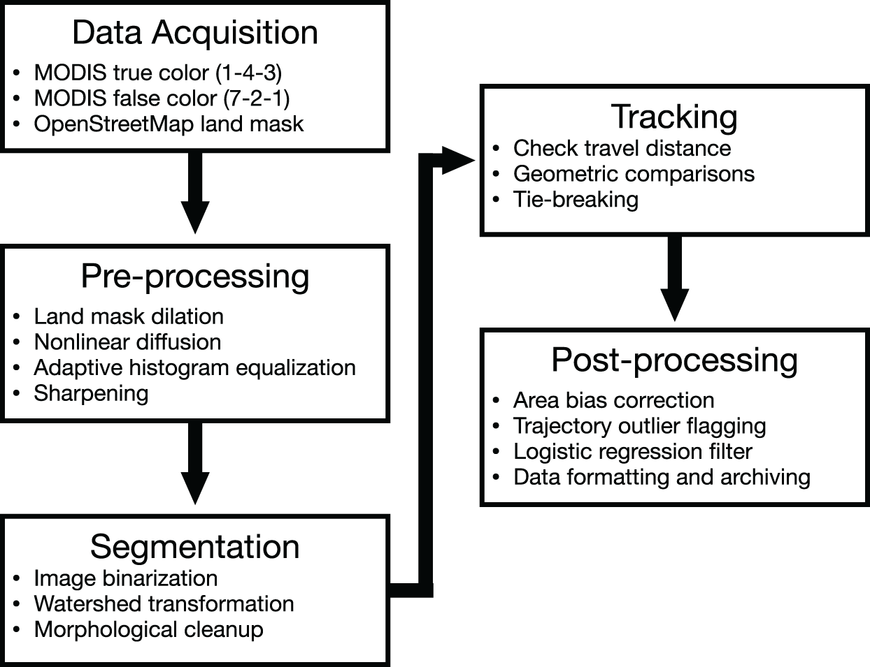


 Open access

