Biased Technical Change

Assuming constant returns to scale in a two-factor production function, a Hicks-neutral technical change is a change that leaves the capital-labor ratio unchanged at constant factor prices.Footnote ⁷ If, instead, the capital-labor ratio increases, the change is said to be labor-saving; if it decreases, it is capital-saving. However, the capital-labor ratio could also change in response to factor price changes.

These two types of change are illustrated in Figure 1. The solid curve represents the initial unit isoquant with output equal to one yard of standard quality cloth. The solid line represents a cost constraint of total cost C ₁ = w L + 1 K and a slope equal to minus w, the relative factor cost when the labor wage is w and the capital rental is normalized to one. The initial cost-minimizing point for unit production is A, where this curve is tangent to the isoquant. At point A, L ₁ is the labor time and K ₁ is the capital amount (loom time). The capital-labor ratio at point A is then K ₁/L ₁. The figure depicts a biased technical change that shifts the unit isoquant to the dashed curve I ₂. At the same relative factor price of w, the cost-minimizing point is now point B. The technical change is labor-saving because it raises the capital-labor ratio from K ₁/L ₁ to K ₂/L ₂.

The figure also shows factor substitution. An increase in the relative wage increases the slope of the cost constraint for the same total cost leading to a switch from constraint C ₁ to constraint C ₃. At the new factor prices, the cost minimization point is D. The capital-labor ratio increases to K ₃/L ₃ as the firm uses more capital and less labor to compensate for the relatively higher labor wage.

Thus a change in the capital-labor ratio could be the result of a biased technical change that shifts the isoquants while holding relative labor and capital prices fixed, or it could be the result of factor substitution that represents movement along the isoquant. However, if economists only observe aggregate data, they cannot usually distinguish between these two changes unambiguously. Indeed, as Peter Diamond, Daniel McFadden, and Miguel Rodriguez show formally, neither the production function nor the path of technical change are identified when empirical researchers only have aggregate data on inputs, outputs, and prices over time, unless some additional structure is assumed.Footnote ⁸ Since most of the research on these questions has been based on aggregate statistics, economists often impose a priori assumptions about the shape of the production function and/or the rate and bias of technical change.

The engineering production function approach avoids this difficulty. Here, the engineering production function specifies the isoquants by determining the labor required per yard of output, L/Y, and the capital required per yard of output, K/Y, where Y is output. Changes in L/Y and K/Y can be decomposed into changes based on new inventions and changes arising from factor substitution. With this decomposition, one can determine how new inventions and factor substitution affected the capital-labor ratio, K/L, as well as output per man-hour, Y/L.

Note that the unit of K is loom time in minutes. This is not a quality adjusted measure of capital because in this exercise I am attributing improvements in quality of capital to technology. Improvements in technology also reduced the nominal price of looms over the course of the century.Footnote ⁹

Mechanization

Weaving is one of many technologies that were mechanized during the early nineteenth century. Mechanization involves the application of machines driven by inanimate power to tasks previously performed by human or animal power. Typically, mechanization brings three main advantages. One, more machines can be used per worker. Weavers can tend more than one loom and spinners can handle hundreds of spindles. Two, machines can be run faster. Three, well-regulated machines can sometimes produce higher-quality goods, for example, finer yarns or more evenly woven cloth.

I focus on the first two advantages and I control for quality by looking at weaving on a relatively standard set of coarse cloths. I consider production of narrow cloths 28–36 inches wide of about 44–64 threads to the inch of weft, using plain weaves, typically sheeting, shirting, or print cloths. I hold output quality constant not because it is unimportant. In fact, the evidence suggests that over the course of the nineteenth century, machines were increasingly able to handle finer yarns, multiple shuttles, and more complex weaves. Rather, I hold quality constant because my focus here is on the sources of increases in capital-labor ratios and these can be more cleanly measured at a given quality level.

Weaving is performed by interlacing two sets of threads, the warp and the weft, at right angles to each other. Many of the weaver's tasks were automated on the first power looms. This automation generally allowed a skilled weaver to tend two power looms at a time instead of one handloom. Also, these power looms generally ran at faster pick rates than those that handloom weavers realized.

Although mechanization reduced the labor required to produce a given output, it did not eliminate the need for labor. There are two reasons. First, some tasks were too difficult to automate, at least initially. For example, when the bobbin ran out of weft yarn, the loom had to be stopped and the empty shuttle replaced by one with a full bobbin. This task was performed manually until the appearance of the Northrop loom at the end of the nineteenth century. Second, the machines were hardly perfect. Effective operation of the looms was sensitive to variation in humidity and temperature and of the quality of raw materials. The machines themselves also were subject to breakdowns and sometimes depended on sensitive adjustments. Yarn would break and shuttles would fly out of the looms or get stuck in the emerging cloth.10 These errors took time to fix. The time to perform tasks, both deterministic and stochastic, determined the capital and labor requirements at each level of technology.

Production with a Single Loom per Weaver

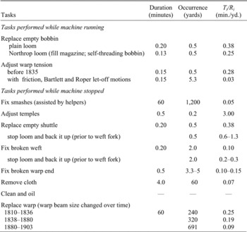
Consider the machine time required per yard of output for a single loom operated by a weaver. Assume, for the moment, that the weaver works without shirking at whatever task needs to be performed and that she works as quickly as a typical skilled weaver. The tasks that a weaver performed on the first power loom circa 1819 are listed in Table 1. In no particular order, the weaver had to replace shuttles and empty bobbins, fix broken warp and weft and smashes, adjust the loom temples (sides of the cloth) and warp tension, and replace the warp and the cloth beam. Over time, various tasks were automated, so that a weaver later in the century no longer performed all of them.

Let the running speed of the loom be s yards per minute. This means that it takes 1/s minutes of loom running time in order to produce a yard of cloth. The weaver would perform some tasks—replace the empty bobbin and adjusting warp tension—while the loom was running. These tasks therefore did not require any additional loom time to complete. However, the weaver would perform other tasks only after the loom was stopped and so these tasks added to the total loom time requirement. For instance, when the shuttle ran out of yarn, the weaver had to stop the loom, replace the shuttle and restart the loom. On coarse cloth, this would occur once half a yard was woven and I estimate that it took a skilled weaver about 0.2 minutes to perform this operation.Footnote ¹¹ This means that for every yard of cloth woven, the weaver would spend 0.2 / 0.5 ≈ 0.4 minutes replacing the shuttle (actually 0.38, as listed in the last column). During the 0.4 minutes, the loom would be stopped and so this contributed to the total loom time requirement. Similar calculations of minutes per yard of cloth produced are shown for the other tasks listed on the bottom portion of Table 1.

TABLE 1

FREQUENCY AND DURATION OF POWER LOOM TASKS

Notes:

See the Appendix for sources.

In other words, the loom time required per yard of output for a skilled weaver operating a single loom with no shirking would be

(1)

where the amount of capital time per yard of cloth (K/Y) is the sum of 1/s, which is the time per yard of cloth when the machine is running, and the second term, which is the time per yard of cloth that the machine stands idle while the worker attends to the machine. N is the total number of tasks that involve stopping the loom (seven not counting cleaning and oiling), T_i is the time to perform each task while the loom is stopped, and R_i is the mean number of yards produced before task i needed to be performed. For tasks such as fixing warp end breaks, these would occur randomly, but on average they occurred every R yards of cloth woven.

Because there is one weaver per loom, it takes as much weaver time to produce a yard of cloth as it takes loom time, that is, L=K. However, it is interesting to look in further detail at the weaver's activity, because she is not actively working all the time.

The weaver is active while performing all of the tasks listed in Table 1, including those that are performed while the loom is running. Therefore, the weaver time per yard of cloth produced can be split into three components

(2)

where T_j is the time it takes to achieve task j while the loom is running, R_j is the mean number of yards produced before task j must be performed, and n is the number of tasks performed while the loom is running, two in this case. W is the time that the weaver watches the loom without actively performing a task.

During the entire production process associated with using a power loom around 1819, which is described in Table 1, the weaver is active for 4.7 minutes for each yard of cloth. However, for a loom running at .044 yards per minute (an estimate for the Waltham mill in 1819), it takes 26.6 minutes of loom time to produce a yard of cloth (K/Y = 26.6). In other words, a weaver operating a single loom would only be active less than a quarter of the time. A key benefit of automation was that a single weaver could operate more than one loom. Additional looms would keep the weaver active for a larger portion of her time.

Engineering Model with Multiple Looms

Adding additional looms introduces a complication. One loom might sit idle while the weaver works on another. With multiple looms, more than one loom might be stopped at any point in time. Each loom will unavoidably be idle and unattended by the worker for some minutes during the production of each yard of cloth. Let the unattended idle time per yard woven be I(k), which increases with the number of looms per weaver, k. Then, following from above, the loom time required to produce one yard of cloth (K/Y) can be written

(3)

When there is only one machine, idle time is zero, I(1) = 0. Adding a second loom allows for the possibility that both looms will be stopped at the same time, so unattended idle time becomes positive with two looms per weaver. Further increases in the number of looms increases the probability that any one loom will sit idle and unattended while one of the k − 1 other looms is being worked on. This means that the more looms assigned per weaver, the longer it takes any one loom to complete a yard of cloth.

Equation 3 gives the loom-minutes required per yard of output, which is the inverse of the output per minute of loom time, Y/K. Similarly, y = Y/L, labor productivity measured as output per weaver-minute, must be the output rate per loom (Y/K) times the number of looms per weaver (k), so that y is a function of k. After substituting from equation 3,

(4)

Additional looms also affect the portion of time that the weaver watches the looms without actively performing a task, W. In the above example with a single loom, the weaver actively performed tasks 4.7 minutes per yard, but it took a total of 26.6 loom minutes to produce a yard, leaving the watch time at 21.9 minutes per yard. With two looms, the weaver would actively perform tasks 2 × 4.7 = 9.4 minutes per yard, leaving a watch time of 17.2 minutes. Thus, watch time W(k) is a decreasing function of the number of looms per weaver, W’(k) < 0.

The tradeoff between labor and capital is captured in the tradeoff between loom idle time, I, and weaver watch time, W. As the number of looms increases, weaver's watch time reaches a limit: the weaver might not be willing or able to work actively 100 percent of the time without rest, hence W does not go to zero. Also, the weaver needs some time to monitor the looms, to respond to errors (it takes some time to walk between 18 looms), and to coordinate activity. Of course, these latter requirements depend on the weaver's willingness to exert effort and skill. If we loosely designate this effort and skill as “labor quality,” q, then watch time can be written as a function of looms per weaver and labor quality, W = W(k, q). Then the weaver time requirement can be written

(5)

Note that as in the equation for a single loom, equation 3, the first two terms are independent of the number of looms per weaver. This is because the tasks that the weaver has to perform on each yard of cloth remain the same regardless of the number of looms that the weaver tends. For example, a task performed every 12 inches on average will still be performed three times per yard regardless of the number of looms tended. Only W changes with the number of looms tended. Since the output rate per weaver must be the inverse of the weaver time required per yard,

(6)

providing an alternative measure of labor productivity.

Duration and Frequency of Tasks

I use two sorts of data to estimate task frequencies and durations. First, for each of the major tasks involved in weaving, I obtained estimates of the time it would take a skilled weaver (mostly circa 1900) to perform each task and of the frequency of occurrence of tasks from trade publications, the Transactions of the National Association of Cotton Manufacturers, patent specifications, and weaving manuals. I also took time-and-motion and measurements on working museum models in Lowell. These estimates are listed in Table 1. Note that where tasks were partially automated, estimates of the duration and frequency both before and after the improvement are included.

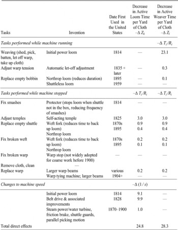
Second, using these sources and additional historical accounts, I compiled a list in Table 2 of the major inventions that automated these tasks, either fully or partially, and those that allowed the looms to run at faster speeds. These changes include both major discrete inventions, such as the weft fork, as well as minor improvements, such as the changes in loom construction that gave the looms greater stability at higher speeds and allowed them to run faster without creating as many defects. For the task of adjusting warp tension, I was able to independently verify the estimate with an econometric analysis of individual weaver monthly productivity from the Lawrence Company.Footnote ¹³

Finally, I also conducted an analysis of how sensitive this model is to changes in task parameters. For example, the most time-consuming task for most of the century was replacing the empty shuttle. This task was automated by the Northrop loom. But a 10 percent change in the frequency of this task, including the time required to stop and back up the loom prior to the adoption of the weft fork, only changes the task time per yard by 0.17 minutes or less, a change of 2 to 3 percent in the weaver time per yard. Ten percent variations in other parameters generated smaller variations.Footnote ¹⁴ This suggests that my estimates of active and idle time are reasonably robust to errors in the task parameter values.

TABLE 2

CHANGES IN LOOM AND WEAVER REQUIREMENTS FROM WEAVING INVENTIONS

Notes:

Changes are in minutes per yard of standard cloth. Weft fork is evaluated for the Lawrence Co., Mill No. 2, in 1855.

Simulation Results for Benchmark Mills

The engineering production function is an instance of a standard operations research problem known as a queuing problem with a finite calling population.Footnote ¹⁵ To simulate the operation of a mill, I assigned a number of weavers each a number of looms and then started running all of these simulated looms. Each loom runs until one of the tasks listed in the top part of Table 1 causes it to stop. The running time after which each task will stop the loom depends on the parameters in Table 1. For some tasks the stopping time is of constant duration, for others, it is a random function of the parameters. Each loom runs until one of its tasks dictates a stop. Then, if the weaver is available, she will attend to the task for the designated duration and then restart the loom. If she is already attending another loom, the newly stopped loom will remain idle until she can attend to it. This process repeats for all the looms and all the weavers for a set period of time. This procedure generates an estimate of the aggregate yards of cloth produced in the simulated mill.

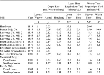
I ran these simulations for a number of benchmark mills from the nineteenth and early twentieth centuries.Footnote ¹⁶ The values from Table 1 are used for the technology configuration of each mill along with historical estimates of loom speeds and looms per weaver.Footnote ¹⁷ In Table 3, I compare the actual output per weaver-minute of each mill, y, calculated as the aggregate yards of cloth for the mill divided by the aggregate labor time, with the value of output per weaver-minute predicted by the simulations, ŷ. As can be seen, the predicted values were quite close to the actual ones. The largest percentage difference was only 0.01/0.06 for the Boston Manufacturing Co. in 1819. The mean error relative to the actual value of y is −0.4 percent, suggesting no substantial bias. The share of the variance in y that is “explained” by the simulation, measured by R², is 0.994 for the 11 observations with both actual and simulated values.

The mills in my sample were presumably selected for comment by contemporaries because they represented the technology frontier. In 1879 mills below that frontier can be compared to typical mills from a supplementary report to the census.Footnote ¹⁸ These are listed as “Five steam-powered mills” and “Six water-powered mills” in Table 3. The productivity of the 5 steam powered mills is quite close to that of Boott Mills, Mill No. 1 in 1876. On the other hand, the water-powered mills likely had older technology and have a substantially lower output per weaver-minute.

TABLE 3

PERFORMANCE AT BENCHMARK MILLS

Notes:

Yards/worker-minute includes labor time of assistants to weavers. W and ∊ are calculated as residuals after estimating times to perform tasks. Simulation results with fractional values of k were calculated by linearly interpolating the two closest integer values.

Sources:

See the Appendix.

The next two columns of Table 3 report the actual loom-minutes per yard for each mill and the estimated number of unattended idle minutes per yard obtained from the simulations. The final two columns report the actual weaver-minutes per yard produced and the estimate of watch time, W, calculated as a residual from equation 5. Some of these values are particularly large and are explored below.

A variety of factors might affect the estimates. Some conditions might have changed over time. For example, weavers at early mills might not have had the same skill level as the weavers whose performances are listed in Table 1. Cotton quality also might have improved over time. If these changes occurred, however, there would be a growing gap between the predicted and actual output rates.Footnote ¹⁹ The fact that the gap did not grow suggests that changes in these factors were not significant.

One of the largest differences between actual and simulated output occurs at the Fall River Ironworks. This might be explained by local conditions where Thomas Young reports an exceptionally low rate of warp end breaks because of extra effort put into warp preparation.Footnote ²⁰ Also, the various benchmark mills in Table 3 produced slightly different cloths with different numbers of threads per inch (from 44 to 64) and different widths (from 28 inches to 36 inches). The later mills in the sample tended to produce narrower widths but with more threads per inch, which had roughly offsetting effects on the weaving task. However, the predicted output rates for the later mills do not appear to be consistently biased one way or the other with respect to cloth parameters. I ran a version of my estimates with adjustments for both of these factors and found that my qualitative conclusions are robust to these adjustments. Also, some weaving tasks were performed by workers other than weavers; I have accounted for this in my estimates for the Northrop looms in 1902/03 because sources clearly indicate that other workers removed cloth and fix smashes.Footnote ²¹

Simulating Loom-Labor Substitution

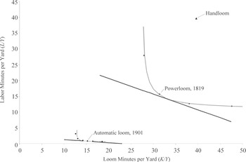
In order to model the effect of factor price changes, it is helpful to simulate production at different capital-labor ratios for a given mill. I do this for two mills, the Boston Manufacturing Company for 1819 and the Merrimack Manufacturing Company, for production using Draper automatic looms in 1901. The data points in Figure 2 show the unit isoquants derived from these two groups of simulations for different numbers of looms per weaver (from 1 to 4 looms per weaver for the 1819 mill and from 4 to 26 looms for the 1901 mill).Footnote ²²Figure 2 also shows the data point for the handloom (here the isoquant is a single point) as well as lines representing constant cost constraints for the relative factor prices in 1819 and 1901 as in Figure 1.

FIGURE 2

SIMULATED UNIT ISOQUANTS

Note: The simulated data points for the first powerloom in 1819 use the parameters for the Boston Manufacturing Company for 1, 2, 3, and 4 looms per weaver. The data points for the automatic loom are for the Merrimack Manufacturing Company for 4, 8, 14, 18, 22, and 26 looms per weaver. The gray curves are derived from nonlinear least squares regressions of the data points in each isoquant using a constant elasticity of substitution production function specification.

Clearly, much of the change between the handloom and the automatic loom of 1901 involves a shift in the isoquants. The cost constraint curves do show evidence of an increase in the relative wage that might encourage a movement along each isoquant—the 1901 curve is more horizontal, indicating a greater relative wage. However, because the isoquants are sharply curved, it does not appear that this movement can account for much change along the vertical axis, namely, change in the weaver time required per yard of output.

This informal observation can be bolstered by a formal quantitative analysis. In order to do this, it is helpful to represent the isoquants as smooth curves rather than just a series of discrete points. The curve might be thought of as an average over many weaving rooms with mixed numbers of looms per weaver. As one example, half the weavers work with two looms and the other half work with three looms. Figure 2 also shows smooth isoquants as thick gray lines between the data points for the mills in 1819 and 1901. These curves were generated by fitting the data points to constant elasticity of substitution (CES) production functions in a nonlinear least squares regression specified in the Appendix. Both curves fit the data points closely with an R Footnote ² of 0.999 in the regression. The estimated elasticity of substitution is 0.23 and 0.26 for 1819 and 1901 respectively. These relatively low elasticities correspond to the sharp curvature of the isoquants seen in Figure 2.

To test the robustness of these estimates, I ran a variety of other simulations for a wide range of parameters typical for nineteenth-century plain looms but using a wide range of loom assignments.Footnote ²³ For all of these simulation runs, I obtained estimates of the elasticity of substitution ranging from 0.09 to 0.26. Also, I ran a regression on monthly output from Lawrence Company Mill No. 2 in Lowell from 1834 through 1855. This regression estimated the elasticity of substitution at 0.14. Finally, these estimates correspond roughly to Ephraim Asher's estimates for the elasticity of substitution for the entire U.S. cotton industry (not just weaving) from 1850–1900 using a CES production function with constant rates of capital- and labor-augmenting technical change.Footnote ²⁴ He obtains estimates of the elasticity of substitution ranging from 0.04 to 0.15. Thus these estimates seem to be similar to a variety of other estimates, if a little higher.

Decomposing Changes

Equations 3 to 6 provide a framework for analyzing the effects of technology and of factor prices on labor productivity, y, and on the bias of technical change. The sources of change in labor productivity can be analyzed by looking at the sources of change in L/Y. The sources of change in the labor-saving bias can be understood by looking at the sources of change in K/Y − L/Y.

Changes in labor time and loom time requirements, Δ(L/Y) and Δ(K/Y), can be decomposed into three components. First, the direct effect of inventions can be shown by changes in loom speed, task duration and task frequency, including the complete automation of a task. Since all of the inventions during this period were directed to reducing the duration and frequency of tasks or increasing loom speed, these changes correspond to the direct effect of inventions on the isoquant and are captured as changes in the times required to adjust the machines while running (T_j), adjust the machines while shut down (T_i), the yards produced before adjustments were required (R_j and R_i), and in the speed of the looms (s). Second, loom-labor substitution driven by factor prices can be shown by changes in the capital-labor ratio attributed to change in the wage to loom price ratio. These can be calculated given estimates of the elasticity of substitution, σ, and the capital share of value added in the weaving process, s_K. In the Appendix, I show that

(7)

Using these formulas, the changes in L/Y and K/Y, that can be attributed to changes in relative factor prices, designated ΔS_l and ΔS_k, respectively, are

(8)

Third, residual changes, M_l and M_k, so that the total changes can be written

(9)

Note also that by applying the difference operator to equations 3 and 5 and comparing the results to equation 9,

(10)

so that changes in loom idle time can be attributed to changes arising from factor substitution plus a residual and changes in weaver watch time can be decomposed into changes arising from factor substitution and a residual.

This framework can be used to quantitatively analyze the changes shown in Figure 2.

Weaving Inventions

Over the course of the nineteenth century there was a dramatic drop in the labor time and loom time needed to produce a yard of cloth. The labor requirement in Table 3, L/Y, fell from 39.6 minutes per yard produced using the handloom circa 1819 to 0.8 minutes per yard produced using Northrop looms circa 1900, a drop of 38.8 minutes per yard. The corresponding loom time per yard, K/Y, fell from 39.6 minutes per yard produced on the handloom to about 14 minutes per yard produced on the Northrop looms, a reduction of just over 25 minutes per yard. From the first power looms at the Boston Manufacturing Company in 1819 to the Northrop loom circa 1900, both the labor time required to produce a yard of cloth and the loom time required to produce a yard of cloth fell about 15 minutes.

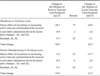
What accounts for these reductions? The decomposition of equation 9 permits us to allocate these changes to the direct effect of weaving inventions, the substitution of looms for labor, and a residual. I calculate the change in each of these components for comparisons of the handloom to the Northrop loom and comparisons of the BMC powerloom to the Northrop loom (see Table 4).

The change attributed to inventions is measured by the change in the minutes the worker was active per yard of cloth and the change in the time that the loom was active per yard of cloth. The nineteenth- century inventions responsible for the main changes in productivity are shown in Table 2, organized by the task that was automated. This list of inventions is described in more depth in the Appendix and it corresponds closely to those inventions mentioned by contemporaries and historians as being important in coarse cotton cloth production.

Drawing on the data in Table 1 and on data about loom speeds, Table 2 shows the direct impact of the various inventions on the loom time required per yard and the labor time required per yard. For example, by automating tasks, the initial power loom reduced labor time per yard by 23.1 minutes, while the increased speed achieved by the initial power loom decreased loom time per yard by 9.1 minutes. The introduction of the self-acting loom temple reduced both loom time and labor time per yard by 3 minutes. The combination of all changes summed to a reduction in weaver minutes per yard of 28.3 minutes and a reduction of loom minutes per yard of 24.8 minutes between the handloom and the mills using Northrop looms in 1901.

TABLE 4

SOURCES OF CHANGE IN LOOM AND LABOR REQUIREMENTS FROM 1819 TO 1901

Sources:

Figures are in minutes per yard. Data from Tables 2 and 3 plus calculation of factor substitution in the text. “Total Change” figures are the sums of differences; these might differ from differences calculated from actual performance in Table 3 because of slight differences between actual and predicted performance.

Loom-Labor Substitution

The loom-labor substitution component is the effect of changes in relative factor prices on the labor time and loom time required per yard of output, ΔS_l and ΔS_k. From equation 8, this requires estimates of the capital share of value added, s_K, the relative wage, w, and the elasticity of substitution, σ. The capital share of value added for the weaving process rises from 46 percent for the Boston Manufacturing Company in 1819 to 64 percent for Merrimack Manufacturing in 1901.

The change in the log of the relative wage is derived from the series for unskilled wages from Paul A. David and Peter Solar and prices of plain looms from historical sources in footnote 9.Footnote ²⁵ These price series capture overall changes in labor and equipment costs that do not reflect changes in the labor quality of weavers or of technical improvements in the looms. The resulting estimate of the effect of loom-labor substitution thus reflects changes in general price levels and not changes in technology and labor quality. The estimated change in the log relative wage is 0.97.

Finally, I use the estimates of elasticity of substitution from the regressions associated with Figure 2 above, 0.23 and 0.26 for 1819 and 1901 respectively. The change in labor time per yard attributed to factor price changes can be calculated using equation 8, however, the effect of movements along the isoquant depend on which isoquant is used. That is,

For the decomposition exercise, I take the average of these two calculations, using ΔS_l = −0.9. Using −1.6 or −0.1 does not substantially change the relative magnitude of the changes resulting from changing factor prices. Repeating the comparable calculation for the effect of factor price changes on the loom time required per yard of output, ΔS_k = 2.6 (an average of 3.8 and 1.4 for 1819 and 1901, respectively).

Residual

Comparing the powerlooms at the Boston Manufacturing Company in 1819 to the Northrop looms in 1901, residual factors account for a decrease of 9.7 minutes of weaver time per yard of output; this corresponds to a substantial drop in weaver watch time, W. Residual factors also account for a drop of 2.1 minutes of loom minutes per yard of output, corresponding to a comparable decrease in the time looms were unattended and idle.

Decomposition of Productivity Changes

A great deal of reduction in weaver time and loom time per yard of output can be directly attributed to inventions. In the comparison of the handloom to the Northrop loom in Table 4, inventions accounted for a 28.3 minute reduction in weaver time per yard and a reduction in loom time per yard of 24.8 minutes. Comparing these figures to the total reduction of weaver time per yard of 38.9 minutes and a reduction of loom time per yard of 24.3 minutes, inventions directly accounted for 73 percent of the reduction in weaver time and virtually all of the reduction in loom time per yard. In comparisons of the first powerlooms at BMC in 1819 to the Northrop looms in 1902, inventions directly accounted for about one-third of the reduction in weaver time per yard(–5.2 minutes of a total of −15.9) and slightly more than the improvement in loom time required per yard(–15.7 of −15.2).

How much of this change can be attributed to movements along the same isoquant, substituting looms for labor in response to changes in relative factor prices? Only 2 percent of the reduction in the labor requirement from the handloom to Northrop loom appears to arise from factor substitution; the change is roughly 6 percent for the comparison of the BMC loom to the Northrop loom.Footnote ²⁶ And, of course, greater capital intensity increased the loom requirement, reducing capital productivity.

The third row in Table 4 shows that a substantial part of the reduction in the labor requirement arises from changes in unaccounted factors. These other factors account for 25 percent of the reduction in the labor requirement between the handloom and the Northrop loom (9.7 yards per minute of 38.9). If, instead, one looks just at the reduction from the Boston Manufacturing Company to the Northrop looms, then 9.7 yards per minute out of a total reduction in weaver time of 15.8 minutes per yard, or 62 percent, can be attributed to other factors. This implies that during the early years, weavers only actively performed tasks about 25–30 percent of the time; by the early twentieth century, weavers at some mills were actively performing tasks 80 percent of the time. Clearly, this is a large and economically significant difference.

Interpreting the Residuals

What might explain the large drop in the weaver's watch time (W) and the smaller drop in the loom idle time (I) after taking into account factor substitution? Technological change is a prime candidate. The various inventions in Table 2 reduced the frequency of loom stoppages and this might have changed both the frequency of loom idle time and weavers’ difficulty in monitoring the looms. By my estimates, a powerloom at the Boston Manufacturing Company in 1819 was stopped every 2.6 minutes on average; a Northrop loom at the benchmark mills in the early 1900s stopped every 33 or 34 minutes. Thus, inventions reduced the frequency of stoppages on each loom, likely accounting for the reduction in loom idle time observed in the residual.

Could these changes in the frequency of stoppages also explain the drop in time that weavers spent watching the looms? Note that the weavers were not simply idle during this time; they were monitoring the looms and the frequency of stoppages might affect the intensity of monitoring. An essential part of their job was to watch for defects in the cloth and errors in the operation of the loom. There were more than a dozen different defects in the cloth that could arise if the loom was not working perfectly and the weaver had to be alert to these and also to breaking threads, empty shuttles etc. so that remedial action could be taken.Footnote ²⁷ In many cases, the longer it took to notice an error, the longer it took to fix because the loom had to be backed up or because one error could cause another, multiplying the severity. Consequently, the weaver's ability to anticipate and to detect errors quickly affected her productivity. Moreover, this was not always easy to do, because many parts of the loom moved faster than the eye could see and many of the cloth defects were subtle to detect, especially in poorly lit factories. And it was likely difficult to maintain a high level of alertness ten or twelve hours a day without some significant resting time.

If errors occurred less frequently, then weavers would not have required as much “buffer” time to notice and respond to errors and the portion of time they spent resting after fixing each error would have been less. However, changes in technology made conditions more difficult for the weavers, not less. While the frequency of stoppages per loom dramatically decreased, the stoppages per weaver actually increased because the weavers were tending that many more looms. Of all the benchmark companies, weavers at the Lawrence Company in 1835 spent the greatest portion of their time watching the looms. Weavers spent the least time watching at the Pacific Mills’ plain looms in 1901–1903. Yet the weaver at the Lawrence Company in 1835 had to tend to a loom stoppage only once every 2.5 minutes on average while a plain loom weaver in 1901–1903 had to tend to a loom stoppage every 0.5 minutes. Thus the weaver in 1901–1903 had to monitor loom stoppages that were five times more frequent while actually spending substantially less time—one-third the time—monitoring the looms.

Only one of the inventions would have affected the visibility of errors: the weft fork stopped the loom when the weft ran out or broke, making the error easier to monitor. However, a rough calculation suggests that the weft fork could not have saved as much as one minute per yard of monitoring time and would have been offset by the higher frequency of stoppages with more looms. Further, weavers without the weft fork at the Lawrence Company in 1855 spent about the same portion of their time watching the looms as the weavers at the Boott Company mill who had the weft fork in 1876. Thus changes in technology likely increased the difficulty of monitoring the looms overall. Technology cannot explain the dramatic drop in the share of time weavers spent watching the looms.

An alternative explanation is that later weavers were able to spend less time monitoring these more frequent stoppages because the later weavers exerted more effort and/or had greater skills at monitoring than did earlier weavers. Several scholars argue that the switch to immigrant mill workers in New England during the 1840s and 1850s allowed mill owners to extract greater effort from the weavers.Footnote ²⁸ Clark's comparisons of weaver productivity across countries also suggest that worker effort was a key factor leading to more output per man-hour.Footnote ²⁹

There are also signs that later weavers had more skill. When the Lowell Mills tried to switch from two looms to three looms per weaver in response to depressed markets in 1842, mill manager James Montgomery thought that most weavers, even experienced ones, could not keep up with three looms.Footnote ³⁰ So the mills had to reduce loom speeds by 15 percent and it took another year until the weavers had apparently acquired the skills necessary to keep up with three looms at the original speed. This change is evident in Table 3, where the watch time per yard produced was cut in half from 6.2 minutes in 1835 to 3.3 minutes in 1845 with no observable change in technology.

It appears that weavers’ skills improved in part because they learned faster. Bessen finds that the “learning curves” for individual weavers at the Lawrence Company were sharply steeper during the 1840s and 1850s than during the 1830s.Footnote ³¹ In monetary terms, the human capital investment per trained weaver of $162 during the later period was more than triple the measure of $47 between 1833 and 1836. As historians and contemporary observers agree that there was little change in the looms between 1835 and 1855, it appears that a substantial portion of the increase in weaver productivity shown in Table 3 was realized through greater weaver skills.Footnote ³² In the period from 1860 to 1900, it appears that skill levels also rose because skilled weavers’ daily wages increased 31 percent relative to the unskilled wage.Footnote ³³

TABLE 5

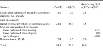
SOURCES OF LABOR-SAVING SHIFT IN ISOQUANTS FROM THE HANDLOOM TO THE NORTHROP LOOM, 1901

Sources:

Data from Table 2 plus calculation of factor substitution in the text (in minutes per yard).

Sources of Technical Bias

Following John Hicks, many economists have observed the large increase in capital-labor ratios accompanying rapid labor productivity growth and concluded that this provides evidence of labor-saving technical change.Footnote ³⁴ Such might seem to be the case for weaving as well. Given the assumption of constant returns to scale, a Hicks-neutral technical change corresponds to a shift in the isoquants that leaves the ratio of the required weaver time per yard, L/Y, to the required loom time per yard, K/Y, unchanged. Since loom time matches weaver time for the handloom, the net bias of technical change over the nineteenth century can be determined by comparing changes in the required weaver time, Δ(L/Y), to required loom time, Δ(K/Y), for producing a yard of cloth. If technical change decreased the weaver's time per yard more than it decreased the loom time per yard, then the net technical change was labor-saving. Thus Δ(K/Y) − Δ(L/Y) provides a measure of the labor-saving bias.Footnote ³⁵

Table 5 shows a simple accounting of the differences in changes in Δ(L/Y) and Δ(K/Y), using the values from Table 4 from the comparison of the handloom to the Northrop loom. The net change, even aside from factor substitution is strongly labor-saving. The time required for a weaver to produce a yard of cloth fell 38.9 minutes while the time required for a loom to produce a yard fell only 24.3 minutes, a difference of 14.6 minutes per yard.

However, decomposing this shift into the terms found in equation 9 yields a surprise. Contrary to assumptions of Hicks and others, only a small part of this increase can be attributed directly to the labor-saving bias of inventions. Instead, inventions exhibit only a small direct labor-saving bias of 3.5 minutes per yard in Table 5. Most of the apparent technical bias appears to arise from the improvement in labor quality as reflected in the decrease of W after taking factor substitution into account.

The literature on “induced innovation” makes the seemingly logical claim that high relative wages should encourage labor-saving inventions. But a closer look shows that technological considerations played a strong role in determining the ultimate bias of technical change. In particular, the breakdown in Table 2 shows that different types of inventions had different effects on the bias. Note that most of the labor-saving shift came from the initial power loom while most of the counterbalancing capital-saving shift came from increases in loom speed. As shown in Table 5, 23.5 minutes per yard in labor-saving were associated with the automation of tasks performed while the loom was running. Of these, 23.1 minutes per yard were tasks automated by the initial power loom as in Table 2. On the other hand, the combined effect of the loom speed changes reported in Table 2 reduced loom time per yard by 20 minutes. This is significant because these were very different sorts of inventions. The initial power loom automated weaving tasks, so this development was highly specific to the field of weaving. These inventions drew on the general vocabulary of machine elements, including cranks, cams, pulley wheels, etc., but they were specific to the textile weaving industry.

On the other hand, much of the improvement in loom speed arose from beneficial developments in other fields, including power transmission, water turbines and steam engines, and improvements in machine construction associated with the development of machine tools and other advances in machining. In other words, much of the capital-saving related to loom speed changes arose from “general purpose technologies.” This meant that inventors developing these technologies sought profits from a wide range of industries in addition to textile weaving. The development costs of the capital-saving inventions were therefore spread over many industries as well. The share of development cost for capital-saving inventions that were amortized to the textile weaving industry might well have been substantially less than the development costs of the industry-specific labor-saving inventions. This means that even if the basic intuition is correct that inventors compared profit against development cost, high relative wages might not have led to a labor-saving bias. Because the development costs of capital-saving inventions were spread over many industries while the development costs of labor-savings inventions had paid for by weaving alone, factor prices might have played only a secondary role in this calculation.

Meanwhile, factor prices might very well have influenced labor quality, as Habakkuk suggested.Footnote ³⁶ Bessen found that high wages relative to prices was important in the mills’ decisions to invest in greater human capital development in the 1840s, which enabled an increase the number of looms per weaver.Footnote ³⁷

In summary, Table 5 illustrates that evidence of a rising capital-labor ratio does not imply that inventions were necessarily labor-saving because the labor in the denominator does not include a measure of human capital. The source of the bias might well have been changes in labor quality rather than inventions. Moreover, because of technological constraints, inventions might not have been particularly labor-saving even if factor prices influenced the choice of inventions that were developed and adopted.