2.1 Models of two-dimensional turbulence

In the QGBT model, relative vorticity $\unicode[STIX]{x1D701}$ is a Lagrangian conserved tracer advected by the geostrophic flow,

where $u=-\unicode[STIX]{x2202}\unicode[STIX]{x1D713}/\unicode[STIX]{x2202}y$ and $v=\unicode[STIX]{x2202}\unicode[STIX]{x1D713}/\unicode[STIX]{x2202}x$ are the two components of the incompressible velocity field $\boldsymbol{u}$ , $\unicode[STIX]{x1D713}$ is the streamfunction and $\unicode[STIX]{x1D701}=\unicode[STIX]{x2202}v/\unicode[STIX]{x2202}x-\unicode[STIX]{x2202}u/\unicode[STIX]{x2202}y=\unicode[STIX]{x1D735}^{2}\unicode[STIX]{x1D713}$ . In horizontal Fourier space, we can write this last equation as

where the hat stands for the Fourier transform and $k$ is the horizontal wavenumber modulus.

Another classical quasi-geostrophic (QG) model is the SQG model, whose potential vorticity is uniform throughout the interior of the fluid (Held et al. Reference Held, Pierrehumbert, Garner and Swanson1995; Lapeyre Reference Lapeyre2017). The system simplifies into a form for which surface temperature $\unicode[STIX]{x1D703}$ is a Lagrangian conserved tracer,

with $\boldsymbol{u}$ defined as above and

(see Held et al. (Reference Held, Pierrehumbert, Garner and Swanson1995) for details of the derivation). Here we considered the non-dimensional form of the equation so as to have a formal resemblance to (2.2).

Starting from these two models, it is possible to consider generalized models, where $q$ is an active tracer obeying

and

with $\unicode[STIX]{x1D6FC}$ a fixed parameter (Pierrehumbert et al. Reference Pierrehumbert, Held and Swanson1994). The case of $\unicode[STIX]{x1D6FC}=2$ corresponds to the QGBT model and $\unicode[STIX]{x1D6FC}=1$ gives the SQG model.

Such models possess generalized energies and enstrophies that are quadratic invariants. The generalized enstrophy expresses the variance of the scalar field $q$ . Our interest will be focused on the cascade of this quantity to small scales. From heuristic arguments, its spectral flux $\unicode[STIX]{x1D702}$ is set by $\unicode[STIX]{x1D702}\propto \unicode[STIX]{x1D70E}_{k}k\,{\mathcal{Q}}(k)$ , where $\unicode[STIX]{x1D70E}_{k}$ is the strain rate responsible for the stirring of the scalar at scale $1/k$ and ${\mathcal{Q}}(k)$ is the shell-averaged spectral density of generalized enstrophy. This last quantity is related to the global tracer variance through $Q=\langle q^{2}\rangle =\int _{0}^{\infty }{\mathcal{Q}}(k)\,\text{d}k$ , the angle brackets indicating an average over space. Assuming that $\unicode[STIX]{x1D70E}_{k}$ depends only on the flow properties at the same local scale $k$ and in the inertial range of the direct cascade of tracer variance, from $\unicode[STIX]{x1D702}=\text{const.}$ one obtains the (shell-averaged) kinetic energy spectrum

for $\unicode[STIX]{x1D6FC}<2$ (Pierrehumbert et al. Reference Pierrehumbert, Held and Swanson1994), where $E(k)$ is related to the total kinetic energy ${\mathcal{E}}$ through ${\mathcal{E}}=\int _{0}^{\infty }E(k)\,\text{d}k$ . As the scaling law was obtained taking into account only local quantities (at scale $k$ ), this regime is associated with local transfers of generalized enstrophy. For $\unicode[STIX]{x1D6FC}\geqslant 2$ the spectral flux no longer explicitly depends on the local wavenumber $k$ , and

(Pierrehumbert et al. Reference Pierrehumbert, Held and Swanson1994; Watanabe & Iwayama Reference Watanabe and Iwayama2004). This regime is associated with non-local generalized enstrophy transfers.

One important consequence of (2.7) is that the strain rate (responsible for the particle pair separation) between $1/k$ and $2/k$ behaves as $k^{2(2-\unicode[STIX]{x1D6FC})/3}$ for $\unicode[STIX]{x1D6FC}<2$ . For these values of $\unicode[STIX]{x1D6FC}$ , the exponent $2(2-\unicode[STIX]{x1D6FC})/3$ is positive and the dispersion of particles separated by a given distance should be controlled by eddies of comparable size. This would be associated with the ‘local dispersion’ regime. In contrast, for $\unicode[STIX]{x1D6FC}\geqslant 2$ , dispersion will be essentially governed by eddies at the largest scales, a regime corresponding to ‘non-local dispersion’. However, one should remember that the presence of nonlinear vortices generally tends to steepen the spectra, so that such phenomenological scalings are only an indication of what could be observed.

2.2 Relative dispersion

The dispersion of passive particles in a turbulent fluid has been widely studied and here we only present its main properties. The reader is referred to reviews by Falkovich et al. (Reference Falkovich, Gaw edzki and Vergassola2001), Sawford (Reference Sawford2001), Bennett (Reference Bennett2006) and Salazar & Collins (Reference Salazar and Collins2009) for broader discussions.

Let us consider $N$ particles whose positions at time $t$ are denoted by $\boldsymbol{x}_{\boldsymbol{i}}(t)$ with $i=1,\ldots ,N$ . Let us examine the pairs $(i,j)$ satisfying $|\boldsymbol{x}_{\boldsymbol{i}}(0)-\boldsymbol{x}_{\boldsymbol{j}}(0)|=y_{0}$ . Then relative dispersion is defined as

where $\langle ~\rangle$ is the average over all of these pairs of particles. The vector $\boldsymbol{y}(t)=\boldsymbol{x}_{\boldsymbol{i}}(t)-\boldsymbol{x}_{\boldsymbol{j}}(t)$ is the separation vector between particles $i$ and $j$ , and $y^{2}=|\boldsymbol{y}|^{2}$ . From this, relative diffusivity can be computed as

with the relative velocity defined by $\unicode[STIX]{x1D6FF}\boldsymbol{v}(t)=\text{d}\boldsymbol{x}_{\boldsymbol{i}}/\text{d}t-\text{d}\boldsymbol{x}_{\boldsymbol{j}}/\text{d}t=\boldsymbol{v}(\boldsymbol{x}_{\boldsymbol{i}}(t),t)-\boldsymbol{v}(\boldsymbol{x}_{\boldsymbol{j}}(t),t)$ . Diffusivity can be rewritten as

with $\boldsymbol{y}_{0}=\boldsymbol{y}(t_{0})$ . Assuming that relative velocity is independent of the particle pair separation, i.e. $\langle \,\unicode[STIX]{x1D739}\boldsymbol{v}(t)\boldsymbol{\cdot }\boldsymbol{y}_{0}\,\rangle =0$ , for time sufficiently small one has

with $\unicode[STIX]{x1D6FF}\boldsymbol{v}_{0}=\unicode[STIX]{x1D6FF}\boldsymbol{v}(t=0)$ . This result was obtained by Batchelor (Reference Batchelor1950) and was confirmed experimentally for 3D turbulent fluids by Bourgoin et al. (Reference Bourgoin, Ouellette, Xu, Berg and Bodenschatz2006) and Ouellette et al. (Reference Ouellette, Xu, Bourgoin and Bodenschat2006). This can be further simplified if one assumes that $y_{0}$ is sufficiently small and that velocity gradients are square-integrable. In that case, the structure function $S(y_{0})=\langle \unicode[STIX]{x1D6FF}\boldsymbol{v}_{0}\boldsymbol{\cdot }\unicode[STIX]{x1D6FF}\boldsymbol{v}_{0}\rangle$ can be replaced by $Zy_{0}^{2}$ , with $Z=\int _{0}^{\infty }k^{2}E(k)\,\text{d}k$ the total relative enstrophy, and

(Babiano et al. Reference Babiano, Basdevant, Roy and Sadourny1990). In the opposite limit of long times, one can expect that particles are separated by a distance larger than the largest eddies and, hence, relative diffusivity converges towards a constant that is twice the absolute diffusivity, due to uncorrelated particle velocities.

At intermediate times, for which dispersion scales are within the inertial range of the tracer variance cascade, the classical assumption of self-similarity for a local turbulent cascade can be made. In that case, diffusivity will depend only on $\unicode[STIX]{x1D702}$ (the spectral turbulent flux of the tracer variance) and $y$ (the distance of pair separation). The turbulent flux scales as $\unicode[STIX]{x1D702}=L^{4-2\unicode[STIX]{x1D6FC}}T^{-3}$ (with $L$ and $T$ being typical length and time scales) and is assumed to be constant in the inertial range of the tracer variance cascade. We then obtain

for $\unicode[STIX]{x1D6FC}<2$ , which implies that

This is a generalization of Batchelor’s (Reference Batchelor1950) result for $\unicode[STIX]{x1D6FC}$ -turbulence. Note that Morel & Larcheveque (Reference Morel and Larcheveque1974) proposed another derivation based on the kinetic energy spectrum $E(k)$ and the dispersion scale. One can apply a hypothesis of local cascade using $(kE(k))^{1/2}/k$ as a diffusivity scale. By self-similarity and for a kinetic energy spectrum $E(k)\propto k^{-\unicode[STIX]{x1D6FD}}$ , one can expect that

Relative dispersion then scales as

Models with $0<\unicode[STIX]{x1D6FC}<2$ satisfy $\unicode[STIX]{x1D6FD}=(4\unicode[STIX]{x1D6FC}+1)/3$ , and (2.14) and (2.15) coincide with (2.16) and (2.17).

Fung & Vassilicos (Reference Fung and Vassilicos1998) discuss the scaling relations obtained by the ‘locality hypothesis’ in their study of kinematic simulations of 2D flows possessing different energy spectra, while Nicolleau & Yu (Reference Nicolleau and Yu2004) adopted a similar approach to examine the scalings in three dimensions. This latter study pointed out the necessity of taking into account finite scale effects due to the initial distance between particle pairs. This was also observed in previous studies dealing with direct numerical simulations of forced 2D turbulence (Babiano et al. Reference Babiano, Basdevant, Roy and Sadourny1990) and we will assess its importance in our simulations.

A different situation occurs when $\unicode[STIX]{x1D6FC}\geqslant 2$ , that is, for sufficiently steep ( $\unicode[STIX]{x1D6FD}\geqslant 3$ ) kinetic energy spectra. In this case the flow is smooth and it can be shown that relative dispersion grows exponentially in time with an exponent related to the maximum Lagrangian Lyapunov exponent of the flow (Falkovich et al. Reference Falkovich, Gaw edzki and Vergassola2001) or, equivalently, to the square root of enstrophy (LaCasce Reference LaCasce2008):

where $c_{1}$ is a non-dimensional constant. Accordingly, one obtains

for the relative diffusivity. This exponential growth of $\langle y^{2}\rangle$ is essentially driven by the largest eddies and it does not depend on the slope of the kinetic energy spectrum. From a Lagrangian point of view this corresponds to a regime of ‘non-local dispersion’.

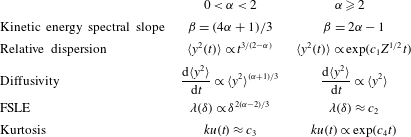
Table 1 summarizes the expected scalings from the type of $\unicode[STIX]{x1D6FC}$ -model used (see §§ 5.2 and 5.3, respectively, for the definitions of FSLE and kurtosis). Note that these scalings do not contradict the initial ballistic regime (2.13) as discussed by Babiano et al. (Reference Babiano, Basdevant, Roy and Sadourny1990) and Nicolleau & Yu (Reference Nicolleau and Yu2004). One interpretation is that, as long as the separation vector does not reorient with respect to the spatial structure of the strain field (in particular the strain axes), the particle pairs retain memory of the initial velocity field, which leads to (2.13).

Equations (2.19) and (2.14) indicate that flows with non-local (respectively local) spectral transfers would imply non-local (respectively local) dispersion. However, the correspondence between transfers and dispersion properties breaks down if either the spectral transfers have both local and non-local contributions, or the energy spectra are steeper than predicted by the theory.

Table 1.

Scaling relations for relative dispersion indicators at intermediate scales as a function of $\unicode[STIX]{x1D6FC}$ (see §§ 5.2 and 5.3, respectively, for the definitions of FSLE and kurtosis). The quantity $Z$ is total relative enstrophy, and $c_{i}$ ( $i=1$ to $4$ ) are constants depending on properties of the fluid flow.

4.1 Active tracer fields

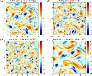
After a transient period (that lasts until $t\approx 36$ ), the statistical properties of the different fields evolve more slowly with the continuous decay of the total energy (see supplementary material available at https://doi.org/10.1017/jfm.2017.253 for more details about the quasi-steadiness of the turbulent regime). Figure 1 presents the active tracer fields for different values of $\unicode[STIX]{x1D6FC}$ at $t=40$ . For $\unicode[STIX]{x1D6FC}=1$ (case of SQG turbulence), we observe intensified coherent structures from the smallest to the largest scales in the active tracer field $q$ (figure 1 a). These small-scale eddies are due to the instability of filaments that are expelled from larger-scale eddies (Held et al. Reference Held, Pierrehumbert, Garner and Swanson1995; Juckes Reference Juckes1995). This clearly also occurs in the case of $\unicode[STIX]{x1D6FC}=1.5$ , e.g. for the filament with $q<0$ that wraps up around the vortex at $(x,y)\approx (-2.2,-1.3)$ (figure 1 b). Going to greater values of $\unicode[STIX]{x1D6FC}$ , we observe the progressive disappearance of these small-scale eddies and the appearance of very long, thin and quasi-passive filaments (see figure 1 c for $\unicode[STIX]{x1D6FC}=2$ ), as also observed by Pierrehumbert et al. (Reference Pierrehumbert, Held and Swanson1994) in forced simulations. As discussed by Held et al. (Reference Held, Pierrehumbert, Garner and Swanson1995), the decay range of the velocity field due to large-scale eddies is much shorter for SQG than for QGBT. Hence the straining processes that suppress the development of the filament instability are less efficient in SQG than in QGBT, which leads to the roll-up of small filaments to form small-scale vortices in SQG. For the viscous run with $\unicode[STIX]{x1D6FC}=1$ , small-scale vortices completely disappear and only large-scale vortices with a few thick filaments remain (figure 1 d).

Figure 1.

Active tracer $q$ at $t=40$ for (a) $\unicode[STIX]{x1D6FC}=1$ , (b) $\unicode[STIX]{x1D6FC}=1.5$ , (c) $\unicode[STIX]{x1D6FC}=2$ and (d) viscous run with $\unicode[STIX]{x1D6FC}=1$ . Values have been normalized by $\langle q^{2}\rangle ^{1/2}$ and the space domain is $[-\unicode[STIX]{x03C0},\unicode[STIX]{x03C0}]^{2}$ .

4.2 Kinetic energy spectra

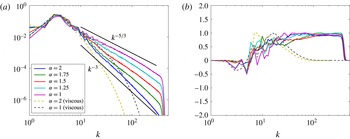
Figure 2(a) presents the kinetic energy spectra for the different simulations averaged over several realizations between times $t=36$ and $t=40$ . At scales below $k=10$ , they share approximately the same shape with a maximum of kinetic energy around $k=4$ . From $k=20$ to $k=200$ , to a good extent, we observe a constant spectral slope in each simulation for the non-viscous runs, while the spectrum rapidly falls off for the two viscous runs. For values of $\unicode[STIX]{x1D6FC}<2$ , the actual slopes are close to the predictions based on local transfer arguments (see table 2). For the case of $\unicode[STIX]{x1D6FC}=2$ the kinetic energy spectrum is observed to be steeper than $k^{-3}$ , probably due to numerical dissipation effects (Boffetta & Ecke Reference Boffetta and Ecke2012).

Figure 2.

(a) Kinetic energy spectra normalized by total energy. (b) Spectral fluxes (normalized by their maximum value) of active tracer variance as a function of $k$ . Spectra and fluxes have been time-averaged over several realizations between $t=36$ and $t=40$ .

Table 2.

Slopes of kinetic energy spectra ( $E(k)\propto k^{-\unicode[STIX]{x1D6FD}}$ ) for different values of $\unicode[STIX]{x1D6FC}$ , computed from a best fit in the range $20\leqslant k\leqslant 200$ . The uncertainties in the fitted values are of the order of $0.05$ . The theoretical slopes correspond to $\unicode[STIX]{x1D6FD}=(4\unicode[STIX]{x1D6FC}+1)/3$ .

4.3 Spectral fluxes and non-locality

To further substantiate the existence of an inertial range with a corresponding direct cascade of active tracer $q$ , we computed the tracer variance flux $\unicode[STIX]{x1D6F1}(K)$ at each wavenumber $K$ :

where the square brackets indicate an average over time and over spectral shells around wavenumber modulus $k$ . The notation $(~)^{\ast }$ stands for the complex conjugate and $\text{Re}(~)$ is the real part. Figure 2(b) presents the spectral flux $\unicode[STIX]{x1D6F1}(K)$ for each case, normalized by its corresponding maximum value. In each simulation we observe that $\unicode[STIX]{x1D6F1}(K)>0$ for $8<K<300$ , which confirms the existence of a direct cascade of active tracer $q$ from large to small scales. Moreover, for most of the simulations, an inertial range (corresponding to constant flux) is found between approximately $K_{min}^{i}=30$ and $K_{max}^{i}=300$ . For some $\unicode[STIX]{x1D6FC}$ cases the plateaus of $\unicode[STIX]{x1D6F1}(K)$ extend less towards the smaller wavenumbers. This might be the reason for the not exactly constant spectral slopes of the corresponding kinetic energy spectra at the lower boundary (in $K$ ) of the inertial range. The two viscous simulations do not possess any inertial range but still exhibit positive flux in a narrower range between $K\approx 8$ and $K\approx 80$ . The absence of a constant energy flux range explains why there is no clear spectral slope for the kinetic energy spectrum (figure 2 a).

To shed more light on the locality of transfers across scales, the tracer variance flux can be decomposed into transfers between modes. For a given wavenumber $k$ , one can look for the scales (associated with wavenumbers $l$ and $m$ ) that contribute to the flux at this scale. In such a situation, we have $\boldsymbol{k}=\boldsymbol{l}+\boldsymbol{m}$ . Such a combination of three scales corresponds to a triadic interaction (Kraichnan Reference Kraichnan1967).

A coarse-grained version of the tracer variance flux $T(n)$ for a circular shell $k_{n}<|\boldsymbol{k}|<k_{n+1}$ can be simply expressed as a triad transfer function from different scales:

where $T(n|a,b)$ represents the flux due to scales $l_{a}<|\boldsymbol{l}|<l_{a+1}$ and $m_{b}<|\boldsymbol{m}|<m_{b+1}$ (see Watanabe & Iwayama (Reference Watanabe and Iwayama2007) for more details). The full expression for $T(n|a,b)$ is given in appendix A.

Figure 3.

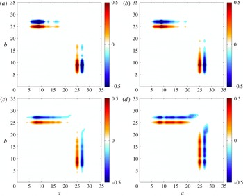
Coarse-grained triad transfer function $T(n|a,b)$ with $n=25$ (corresponding to $k=95$ ); the horizontal and vertical axes respectively correspond to the shell indices $a$ and $b$ . Cases with (a) $\unicode[STIX]{x1D6FC}=2$ , (b) $\unicode[STIX]{x1D6FC}=1.75$ , (c) $\unicode[STIX]{x1D6FC}=1.5$ and (d) $\unicode[STIX]{x1D6FC}=1$ . Transfers have been time-averaged and normalized by the total tracer variance dissipation.

The transfer function $T(n|a,b)$ is shown in figure 3 (for $n=25$ ); here $k_{n}=\unicode[STIX]{x1D706}^{n}$ , $l_{a}=\unicode[STIX]{x1D706}^{a}$ , $m_{b}=\unicode[STIX]{x1D706}^{b}$ and $\unicode[STIX]{x1D706}=1.2$ . The index $n=25$ corresponds to the shell centred on wavenumber 95, which is in the inertial range. For $\unicode[STIX]{x1D6FC}=2$ and $\unicode[STIX]{x1D6FC}=1.75$ , we see that spectral transfers are due to triads with $a\ll b$ or $a\gg b$ . This means that nonlinear transfers between triads are mostly non-local in these cases. While for $\unicode[STIX]{x1D6FC}=2$ this is expected from the theory, this is less so when $\unicode[STIX]{x1D6FC}=1.75$ . In contrast, for $\unicode[STIX]{x1D6FC}=1$ and $\unicode[STIX]{x1D6FC}=1.5$ , triads with $a\approx b$ also contribute to the transfer function. In these two cases (in particular the SQG case), it has to be stressed that both local and non-local triads are responsible for the transfers while the phenomenological theory would advocate for only local contributions. Watanabe & Iwayama (Reference Watanabe and Iwayama2007) obtained the same results for the cases $\unicode[STIX]{x1D6FC}=1$ and $\unicode[STIX]{x1D6FC}=2$ in forced simulations. Hence, this result suggests that locality and non-locality in terms of turbulent energy transfers are not as exclusive as one might think a priori.

4.4 Locality of the strain field

The quantity that will matter in the dispersion of particles is the strain rate, as this governs the stirring of fluid parcels (see Lapeyre (Reference Lapeyre2002) for a discussion on Lagrangian strain rates). A way to determine if a particular scale $k$ will be strained by eddies of comparable size or by larger ones is to compute the weight of the strain rate at a given scale relative to the strain rate at larger scales. To this end we introduce the enstrophy ratio $R_{k}$ :

where the infrared cutoff $k_{min}>0$ corresponds to the smallest wavenumber resolved in the domain, or the wavenumber containing the largest enstrophy at large scale. Here the numerator represents the local strain rate (more precisely the enstrophy $l^{2}E(l)$ ) contained in eddies with size between $k/2$ and $k$ , while the denominator expresses the strain rate by larger-scale structures felt by a given scale $k$ (assuming that smaller-scale motions will not contribute to the stirring of larger-scale structures). Using a power-law spectrum $E(k)\sim k^{-(4\unicode[STIX]{x1D6FC}+1)/3}$ , the quantity $R_{k}$ is equal to $R_{k}=(1-2^{4(\unicode[STIX]{x1D6FC}-2)/3})/(1-(k_{min}/k)^{4(2-\unicode[STIX]{x1D6FC})/3})$ and tends to $R^{lim}=1-2^{4(\unicode[STIX]{x1D6FC}-2)/3}$ when $k$ is large enough for $\unicode[STIX]{x1D6FC}<2$ . For $\unicode[STIX]{x1D6FC}=2$ , $R_{k}$ decays as $R_{k}=\log 2/\log (k/k_{min})$ . Hence at large $k$ , small eddies of size $1/k$ do not contribute to the stirring when $\unicode[STIX]{x1D6FC}=2$ whereas they have a non-negligible impact for $\unicode[STIX]{x1D6FC}<2$ .

Figure 4.

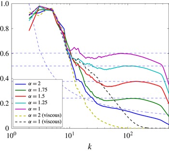
Ratio, $R_{k}$ , of enstrophy contained in $[k/2,k]$ to enstrophy contained in $[k_{min},k]$ . The horizontal dashed curves correspond to the theoretical predictions $R^{lim}$ , while the decreasing one is $R_{k}=\log 2/\log (k/k_{min})$ .

Figure 4 presents the quantity $R_{k}$ along with its theoretical limit (dashed lines). At large scales, $R_{k}$ is close to 1 for all cases, as can be understood from its definition in the limit of small wavenumbers. For smaller scales, namely those corresponding to $k>30$ , $R_{k}$ decreases in fair agreement with the theoretical prediction for $\unicode[STIX]{x1D6FC}=2$ , while it approaches a constant value for $\unicode[STIX]{x1D6FC}<2$ . This value is close to $1-2^{4(\unicode[STIX]{x1D6FC}-2)/3}$ . As $\unicode[STIX]{x1D6FC}$ decreases, local scales have a more and more important weight in the strain rate. However, $R_{k}$ only reaches $60\,\%$ of the total strain for $\unicode[STIX]{x1D6FC}=1$ . This indicates that larger scales still provide a non-negligible contribution to the stirring for the SQG case and raises the possibility that a dispersion theory based on local arguments might not be sufficient to account for the different processes involved in the dispersion.

5.1 Time-dependent statistics

As previous studies showed (Babiano et al. Reference Babiano, Basdevant, Roy and Sadourny1990; Boffetta & Sokolov Reference Boffetta and Sokolov2002; Nicolleau & Yu Reference Nicolleau and Yu2004; Bourgoin et al. Reference Bourgoin, Ouellette, Xu, Berg and Bodenschatz2006), relative dispersion statistics depend on the initial particle pair separation $y(t=0)=y_{0}$ . It is then useful to introduce the wavenumber $k_{0}=2\unicode[STIX]{x03C0}/y_{0}$ , which allows one to compare the initial pair separation with the typical length scales associated with the inertial range of the active tracer cascade. In the following we will take $k_{0}=512$ , corresponding to initial separations $y_{0}\approx 1.23\times 10^{-2}$ , smaller than the scale at which the tracer variance flux vanishes and the kinetic energy rapidly drops to zero, namely $k_{v}\approx 350$ . We have also performed a particle release experiment with $k_{0}=1024$ but tracking particles over a more limited time period, and we obtained qualitatively similar results.

We further introduce a time scale corresponding to the time at which particle pairs have forgotten their initial separation, i.e. their early behaviour (see (2.12)). Such a time scale will take into account the period during which particles lose ‘memory’ of their initial position and velocities, which would delay the onset of scaling relations (see discussion in Babiano et al. Reference Babiano, Basdevant, Roy and Sadourny1990). For that purpose, we introduce a ‘memory index’,

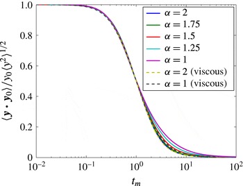
and we look for times $t$ such that $M(t)\approx 0$ . Figure 5 shows such a quantity in the case of $k_{0}=512$ . Here, we rescaled time as $t_{m}=t/\unicode[STIX]{x1D70F}_{m}$ , where $\unicode[STIX]{x1D70F}_{m}$ is such that $M(t=\unicode[STIX]{x1D70F}_{m})=0.5$ for each value of $\unicode[STIX]{x1D6FC}$ . We clearly observe that the separation distance decorrelates with its initial value in the same manner for all simulations, provided the appropriate time scale $\unicode[STIX]{x1D70F}_{m}$ is used to make time non-dimensional. The cases $\unicode[STIX]{x1D6FC}=1$ and $1.25$ seem to decorrelate more slowly in time but the difference with the other cases remains quite small. Hence, the time scale $\unicode[STIX]{x1D70F}_{m}$ seems to provide the typical time scale of decorrelation with the initial conditions, and in the following we will use $t_{m}$ as the rescaled time for an appropriate comparison of the different cases. We note that another time scale $T_{z}=Z^{-1/2}$ , based on the relative enstrophy $Z$ , could be appropriate. We found that this time scale is highly correlated with $\unicode[STIX]{x1D70F}_{m}$ since the ratio $T_{z}/\unicode[STIX]{x1D70F}_{m}$ stays between $0.5$ and $0.8$ for the different cases (not shown). However, $t_{m}$ was found to give better agreement between the different simulations.

Figure 5.

Particle separation memory index $M(t)=\langle \boldsymbol{y}\boldsymbol{\cdot }\boldsymbol{y}_{0}\rangle /y_{0}\langle y^{2}\rangle ^{1/2}$ as a function of the renormalized time $t_{m}=t/\unicode[STIX]{x1D70F}_{m}$ . Initial pair separations correspond to $k_{0}=2\unicode[STIX]{x03C0}/y_{0}=512$ .

Figure 6.

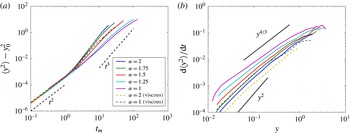
(a) Relative dispersion (after subtraction of the initial value) $\langle y^{2}\rangle -y_{0}^{2}$ as a function of time $t_{m}$ . (b) Diffusivity $\text{d}\langle y^{2}\rangle /\text{d}t$ as a function of $\langle y^{2}\rangle ^{1/2}$ . In this panel, only data with $M(t)<0.5$ have been plotted. In each case, the initial separation $y_{0}$ corresponds to $k_{0}=512$ .

For short times ( $t_{m}\ll 1$ ), we expect relation (2.12) to hold. Figure 6(a) clearly indicates that this regime is observed up to a time $t_{m}\approx 1$ . This is in agreement with other studies (Nicolleau & Yu Reference Nicolleau and Yu2004; Bourgoin et al. Reference Bourgoin, Ouellette, Xu, Berg and Bodenschatz2006). We note that simulations with different values of $\unicode[STIX]{x1D6FC}$ and $k_{0}$ give exactly the same typical law $\langle y^{2}\rangle \approx y_{0}^{2}(1+ct_{m}^{2})$ for sufficiently small $t_{m}$ , with $c$ a constant independent of $\unicode[STIX]{x1D6FC}$ and $k_{0}$ – see the good collapse of the different curves in figure 6(a) when varying $\unicode[STIX]{x1D6FC}$ at fixed $k_{0}$ and figure 7 when varying $k_{0}$ at fixed $\unicode[STIX]{x1D6FC}$ . This indicates that $\unicode[STIX]{x1D70F}_{m}$ is the relevant time scale for comparing the different simulations. For each value of $\unicode[STIX]{x1D6FC}$ the departure from the ballistic regime seems to occur around a common value between $t_{m}=1$ and $t_{m}=2$ . At that time, the dispersion scale is of the order of $y^{2}\approx (2\unicode[STIX]{x03C0}/K_{max}^{i})^{2}\approx 4.4\times 10^{-4}$ , i.e. in the inertial range.

We now turn to intermediate times for which the dispersion should obey a power law $\langle y^{2}\rangle \propto t^{3/(2-\unicode[STIX]{x1D6FC})}$ for $\unicode[STIX]{x1D6FC}<2$ and an exponential law for $\unicode[STIX]{x1D6FC}=2$ and the viscous runs (table 1). Figure 6(a) shows that relative dispersion increases more rapidly when $\unicode[STIX]{x1D6FC}$ increases, as expected. However, $\langle y^{2}\rangle$ is systematically found to grow in time more slowly than predicted by the theory. 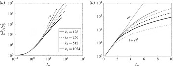A difficulty in measuring the power-law exponents (or exponential growth rates) is due to the fact that they strongly depend on $k_{0}$ , and they typically increase with it. Figure 7 displays $\langle y^{2}\rangle /y_{0}^{2}$ as a function of time for different $k_{0}$ when $\unicode[STIX]{x1D6FC}=1$ (a) and $\unicode[STIX]{x1D6FC}=2$ (b). In both cases, we see that the asymptotic dispersion regime is better realized when increasing $k_{0}$ . For $\unicode[STIX]{x1D6FC}=1$ (figure 7 a), relative dispersion tends to approach the theoretical expectation $\langle y^{2}\rangle \sim t^{3}$ when $y_{0}$ is decreased, but the scaling is still limited to a quite short range even for the smallest $y_{0}$ considered. On the other hand, for $\unicode[STIX]{x1D6FC}=2$ (figure 7 b), after a growth in $1+ct_{m}^{2}$ up to $t_{m}\approx 1$ , the time evolution of relative dispersion might suggest an exponential law, but only visible for smaller and smaller values of $y_{0}$ and up to a time $t_{m}\approx 2$ . Such difficulties in observing clear scalings relating relative dispersion with time were noted by numerous authors (Morel & Larcheveque Reference Morel and Larcheveque1974; Boffetta & Sokolov Reference Boffetta and Sokolov2002; Jullien Reference Jullien2003; Nicolleau & Yu Reference Nicolleau and Yu2004). Here two reasons can be invoked. Relative dispersion $\langle y^{2}\rangle$ involves particle pairs with different histories: some may separate more slowly than others, e.g. if they are trapped inside coherent vortices. This can lead to spurious behaviours due to averaging together, at fixed time, potentially very different pair separations (Artale et al. Reference Artale, Boffetta, Celani, Cencini and Vulpiani1997). Another possible reason lies in the weakly non-stationary character of the turbulent flow; indeed, relative enstrophy slowly decreases in time, causing a temporal variation of the exponential growth rate of the squared separation for $\unicode[STIX]{x1D6FC}=2$ .

Figure 7.

Relative dispersion as a function of time $t_{m}$ for different values of $y_{0}$ (with $k_{0}=2\unicode[STIX]{x03C0}/y_{0}$ ) for $\unicode[STIX]{x1D6FC}=1$ (a) and $\unicode[STIX]{x1D6FC}=2$ (b). Here $d$ is a constant proportional to the square root of relative enstrophy.

Figure 8.

Compensated diffusivity $\text{d}\langle y^{2}\rangle /\text{d}t\times \langle y^{2}\rangle ^{-(\unicode[STIX]{x1D6FC}+1)/3}$ as a function of $\langle y^{2}\rangle ^{1/2}$ . Panels (a–e)  $\unicode[STIX]{x1D6FC}=1,1.25,1.5,1.75,2$ . Panel (f) is the viscous case $\unicode[STIX]{x1D6FC}=2$ . The different curves correspond to different values of initial separation distance.

5.2 Scale-dependent statistics

Statistics at fixed scale are preferable to avoid the superposition of different dispersion regimes due to particle pairs having different histories (Morel & Larcheveque Reference Morel and Larcheveque1974; Bennett Reference Bennett1984; Aurell et al. Reference Aurell, Boffetta, Crisanti, Paladin and Vulpiani1997; LaCasce & Bower Reference LaCasce and Bower2000).

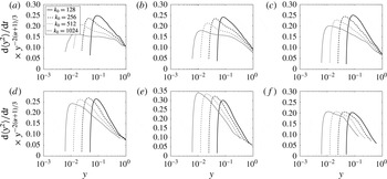
Figure 6(b) shows relative diffusivity $\text{d}\langle y^{2}\rangle /\text{d}t$ as a function of pair dispersion $y=\langle y^{2}\rangle ^{1/2}$ for an initial separation corresponding to $k_{0}=512$ . Only data for which the particle pairs have forgotten their initial separation (i.e. $t>\unicode[STIX]{x1D70F}_{m}$ ) have been plotted. The existence of a power-law regime appears more clearly when using this indicator. To better estimate the correspondence with the theory, a compensated plot $\text{d}\langle y^{2}\rangle /\text{d}t\times \langle y^{2}\rangle ^{-(\unicode[STIX]{x1D6FC}+1)/3}$ can be examined (figure 8). When decreasing the initial separation distance $y_{0}$ (or increasing $k_{0}$ ) for $\unicode[STIX]{x1D6FC}<2$ , we see that a regime of quasi-constant compensated diffusivity (i.e. a broadening of the main peak) appears. This is more true when $\unicode[STIX]{x1D6FC}$ is small and when $k_{0}$ is large. In particular, for $\unicode[STIX]{x1D6FC}=1$ and $\unicode[STIX]{x1D6FC}=1.25$ (figure 8 a,b), we clearly see that the compensated diffusivity becomes constant over a large range of $y$ . Note also that for the viscous case $\unicode[STIX]{x1D6FC}=2$ , a restricted range of constant compensated diffusivity appears (figure 8 f). For these different cases, we are confident that the dispersion statistics obey scaling laws predicted by the self-similarity theory based on a local cascade. However, this is only confirmed for small enough $y_{0}$ . For $\unicode[STIX]{x1D6FC}=2$ , the compensated diffusivity does not show a clear plateau even for $k_{0}=1024$ (figure 8 e). A similar conclusion is obtained for the viscous case $\unicode[STIX]{x1D6FC}=1$ (not shown).

With regard to the difficulty of observing exponential growth when $\unicode[STIX]{x1D6FC}=2$ , an alternative diagnostic is the characteristic time of relative dispersion, defined in Babiano et al. (Reference Babiano, Basdevant, Roy and Sadourny1990) as

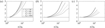
A constant value of $\unicode[STIX]{x1D70F}_{exp}(y)$ corresponds to an exponential separation and defines the range of separations over which this regime is found. The behaviour of this quantity for different initial separations is presented in figure 9, again for $\unicode[STIX]{x1D6FC}=1$ , $\unicode[STIX]{x1D6FC}=2$ and the viscous run with $\unicode[STIX]{x1D6FC}=2$ . We have rescaled $\unicode[STIX]{x1D70F}_{exp}$ with its minimum value in each case and only data in the inertial range are shown. For $\unicode[STIX]{x1D6FC}=1$ , we do not expect an exponential regime and this serves to contrast with the other two cases. Indeed, in this case, the time scale $\unicode[STIX]{x1D70F}_{exp}$ increases very rapidly with $y$ (figure 9 a), which indicates that an exponential growth is not present for the values of $y_{0}$ considered. For $\unicode[STIX]{x1D6FC}=2$ the characteristic time $\unicode[STIX]{x1D70F}_{exp}$ is found to be constant, or at least to vary weakly (between $1$ and $2$ ) over a broader range of scales (almost a decade in $y$ for the smallest $y_{0}$ ). This strongly suggests that non-local dispersion is taking place in the inertial range. As can be seen, the smaller the initial separation, the larger the range of separations for which $\unicode[STIX]{x1D70F}_{exp}(y)=\text{const.}$ , consistent with Babiano et al. (Reference Babiano, Basdevant, Roy and Sadourny1990). In contrast to the $\unicode[STIX]{x1D6FC}=1$ case, the minimum of $\unicode[STIX]{x1D70F}_{exp}$ was found to be independent of $y_{0}$ (not shown). The viscous run with $\unicode[STIX]{x1D6FC}=2$ reveals a much clearer exponential range, indicating that steeper energy spectra are accompanied by more non-local dispersion.

Figure 9.

Characteristic time of relative dispersion $\unicode[STIX]{x1D70F}_{exp}$ as a function of $y/y_{0}$ for $\unicode[STIX]{x1D6FC}=1$ (a), $\unicode[STIX]{x1D6FC}=2$ (b) and the viscous run with $\unicode[STIX]{x1D6FC}=2$ (c). Only data for which $y$ is within the inertial range are displayed and $t_{m}>1$ . The value $\unicode[STIX]{x1D70F}_{exp}$ has been rescaled by its minimum value. For $k_{0}=1024$ the inertial range occurs from $y/y_{0}>3.4$ , while it is below $2$ for the other values of $k_{0}$ .

Another way to diagnose local/non-local dispersion is to investigate the exponential growth rate of separation, not as a function of time, but scale by scale. To this end, one can measure the time $\unicode[STIX]{x1D70F}(\unicode[STIX]{x1D6FF})$ needed to observe the growth of separation from a scale $\unicode[STIX]{x1D6FF}$ to a scale $r\unicode[STIX]{x1D6FF}$ (with $r>1$ ). The finite-size Lyapunov exponent (FSLE) is then defined as

where the angular brackets indicate an average over all particle pairs (Artale et al. Reference Artale, Boffetta, Celani, Cencini and Vulpiani1997; Aurell et al. Reference Aurell, Boffetta, Crisanti, Paladin and Vulpiani1997). If the kinetic energy spectrum scales as $k^{-\unicode[STIX]{x1D6FD}}$ , the FSLE is expected to be given by

for $\unicode[STIX]{x1D6FD}<3$ . The power-law dependence as a function of $\unicode[STIX]{x1D6FC}$ is then

when $\unicode[STIX]{x1D6FC}<2$ . For spectra steeper than $k^{-3}$ or for $\unicode[STIX]{x1D6FC}\geqslant 2$ , $\unicode[STIX]{x1D706}(\unicode[STIX]{x1D6FF})$ should reach a constant value. In such a case of scale-independent FSLE, dispersion is controlled by non-local processes, that is, by velocity field features at much larger scales than the particle separation. In the limit of infinitesimal separation, $\unicode[STIX]{x1D706}(\unicode[STIX]{x1D6FF})$ converges to the maximum Lagrangian Lyapunov exponent $\unicode[STIX]{x1D706}_{L}$ of the flow.

In our different simulations, the FSLE was computed using the scale separation factor $r=1.2$ , original pairs and the time of first crossing technique, but the results were qualitatively the same using chance pairs or the fastest crossing method (Lumpkin & Elipot Reference Lumpkin and Elipot2010). Consistent with Özgökmen et al. (Reference Özgökmen, Poje, Fischer, Childs, Krishnan, Garth, Haza and Ryan2012), we rescaled FSLE with the Okubo–Weiss parameter $Q$ (Okubo Reference Okubo1970; Weiss Reference Weiss1991) that characterizes hyperbolic regions of the flow.

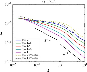
The behaviour of the FSLE is displayed in figure 10. For $0.03<\unicode[STIX]{x1D6FF}<0.3$ , approximately corresponding to $20<k<200$ , i.e. in the wavenumber range where constant spectral slopes were detected (see figure 2 a), we observe a power law $\unicode[STIX]{x1D706}(\unicode[STIX]{x1D6FF})\propto \unicode[STIX]{x1D6FF}^{-\unicode[STIX]{x1D6FE}}$ with an exponent $\unicode[STIX]{x1D6FE}$ that decreases as the slope of the kinetic energy spectrum increases (see table 3). This is in qualitative agreement with the theory but we remark that the decrease of $\unicode[STIX]{x1D706}(\unicode[STIX]{x1D6FF})$ with $\unicode[STIX]{x1D6FF}$ is slightly slower than expected for $\unicode[STIX]{x1D6FC}=1$ and $\unicode[STIX]{x1D6FC}=1.25$ . At scales smaller than $\unicode[STIX]{x1D6FF}=0.03$ , $\unicode[STIX]{x1D706}(\unicode[STIX]{x1D6FF})$ displays some tendency to flatten in all cases, but no clear plateau region allowing the measurement of $\unicode[STIX]{x1D706}_{L}$ is detected, at least for $\unicode[STIX]{x1D6FC}\leqslant 1.75$ . The cases with $\unicode[STIX]{x1D6FC}=2$ and the two viscous runs present a considerably weaker scale dependence, with almost constant FSLE up to scales $\unicode[STIX]{x1D6FF}\approx 0.5$ , pointing to an essentially non-local dispersion regime. Notice that the steepening of the FSLE for $\unicode[STIX]{x1D6FF}<0.1$ for the viscous run with $\unicode[STIX]{x1D6FC}=1$ may be due to the fact that particles at small separation slowly forgot their initial separation. Finally, independently of the value of $\unicode[STIX]{x1D6FC}$ , for $\unicode[STIX]{x1D6FF}>1$ we observe a faster decrease with $\unicode[STIX]{x1D6FF}$ of the FSLE, but the behaviour of these scales $\unicode[STIX]{x1D6FF}>\unicode[STIX]{x03C0}$ may be misleading, as periodicity in the velocity field may modify the dispersion properties.

Figure 10.

FSLE (rescaled by the Okubo–Weiss parameter) computed from original pairs with particles regularly spaced every $2\unicode[STIX]{x03C0}/512$ in each direction. Regimes $\unicode[STIX]{x1D706}\propto \unicode[STIX]{x1D6FF}^{-2/3}$ and $\unicode[STIX]{x1D706}\propto \unicode[STIX]{x1D6FF}^{-1}$ are indicated for comparison.

Table 3.

Slopes of FSLE $\unicode[STIX]{x1D706}(\unicode[STIX]{x1D6FF})$ computed in the range $0.03<\unicode[STIX]{x1D6FF}<0.3$ (with uncertainties of the order of $0.05$ ) and comparison with predictions based on $\unicode[STIX]{x1D6FC}$ .

5.3 Higher-order statistics

Relative dispersion is the second-order moment of particle pair separation. While for Gaussian probability distributions knowledge of it provides a good characterization of the statistics, this is no longer true for strongly non-Gaussian distributions, such as those typically encountered in turbulence. In such a case it is useful to compute higher-order moments or the probability density function (p.d.f.) itself. As discussed in detail by Bennett (Reference Bennett1984) and LaCasce (Reference LaCasce2010), the shapes of p.d.f.s give substantial information to determine what kind of dispersion regime is present.

In a 2D homogeneous incompressible flow the p.d.f. of pair separation $P(y,t)$ evolves according to the following Fokker–Planck equation (Richardson Reference Richardson1926):

where $y$ is the pair separation (Bennett Reference Bennett1984; LaCasce Reference LaCasce2010). Equation (5.6) must be supplemented by an initial condition such as, for example,

For a diffusivity $K_{rel}=\unicode[STIX]{x1D705}y^{a}$ with $a<2$ , using the Laplace transform one can find the general solution

where $\text{I}_{n}$ is the modified Bessel function of order $n$ . In the limit of large distances but before the final diffusive range ( $y\gg y_{0}$ and $\unicode[STIX]{x1D705}t\gg y^{2-a}$ ), one has

which is known as the Richardson p.d.f. for $a=4/3$ . In contrast, when $a=2$ , the law is log-normal, and it is known as the Lundgren p.d.f. (Lundgren Reference Lundgren1981):

where the time scale $T$ is proportional to the inverse cube root of the enstrophy dissipation rate (Lin Reference Lin1972). Note that if one uses $K_{rel}=\unicode[STIX]{x1D705}t^{b}$ instead of $K_{rel}=\unicode[STIX]{x1D705}y^{a}$ in (5.6), a different p.d.f. can be obtained, in particular a Gaussian form in three dimensions for $b=3$ (Batchelor Reference Batchelor1952a ). In 3D turbulent experiments, Ouellette et al. (Reference Ouellette, Xu, Bourgoin and Bodenschat2006) showed the dependence of the observed p.d.f. on the initial pair separations, which suggests that in particular cases (5.8) is preferable to (5.9) when comparing with observations.

Figure 11.

Probability density functions of pair separations for (a) $\unicode[STIX]{x1D6FC}=2$ and (b) $\unicode[STIX]{x1D6FC}=1$ at different values of $t_{m}$ . In panel (a), the p.d.f.s are shown as a function of the rescaled variable $(y/y_{0})^{1/\unicode[STIX]{x1D70E}}=\exp [(1/\unicode[STIX]{x1D70E})(\log y-\log y_{0})]$ , where $\unicode[STIX]{x1D70E}$ is the standard deviation of the p.d.f. in log space. The Lundgren distribution is represented by the black dashed curve. In panel (b), the p.d.f.s are shown as a function of $y/y_{0}$ . The dashed lines correspond to the Richardson solutions. In all cases the initial separation of particle pairs corresponds to $k_{0}=512$ .

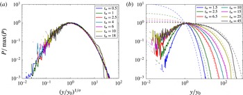
Figure 11 presents the p.d.f. observed at different times, and with $k_{0}=2\unicode[STIX]{x03C0}/y_{0}=512$ , for the two extreme cases (a)  $\unicode[STIX]{x1D6FC}=2$ (QGBT) and (b)  $\unicode[STIX]{x1D6FC}=1$ (SQG) corresponding to $a=2$ and $a=4/3$ , respectively.

Figure 11(a) indicates that the case $\unicode[STIX]{x1D6FC}=2$ is representative of a Lundgren law, at least for $t_{m}\leqslant 10$ . Note that the correction $2t/T$ in (5.10) was found to be small. The adequacy of the Lundgren law in representing the dispersion p.d.f. provides strong support for non-local dispersion, in a more unambiguous way than the dispersion, diffusivity or FSLE. For larger times and $y$ much larger than its initial value, the p.d.f. is less well approximated by this law. This particularly occurs for the right tail of the p.d.f. even at $t_{m}>6$ and is in agreement with the fact that at such times the exponential dispersion law is not observed (figure 7 b). In the case $\unicode[STIX]{x1D6FC}=1$ (figure 11 b), the separation p.d.f. substantially differs from the Lundgren solution compared to the other case but is reasonably well captured by the prediction of (5.9) with $a=4/3$ , corresponding to a Richardson distribution, in the range $6.5\leqslant t_{m}\leqslant 25$ . The strong fluctuations of the p.d.f.s visible in figure 11(a,b) for $y<y_{0}$ are due to limited statistics at very small separations.

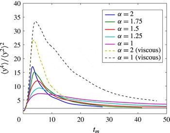
The p.d.f. allows one to compute all moments such as, for example, relative dispersion. Interesting information is also provided by the kurtosis of relative displacements, which samples the high tails of the distribution corresponding to rare and very large particle separations. It is defined as

For a Rayleigh distribution (the expected one for a normally distributed random process and in the diffusive limit of dispersion), $ku=2$ (LaCasce Reference LaCasce2010). In the Richardson regime, the kurtosis would attain a value close to $5.6$ , while it would exponentially grow in time in the (marginally) non-local regime of the enstrophy cascade (associated with exponential growth of relative dispersion) as shown by LaCasce (Reference LaCasce2010).

Figure 12.

Relative displacement kurtosis as a function of $t_{m}$ ; here $k_{0}=512$ . The black thin line corresponds to a kurtosis of $\langle y^{4}\rangle /\langle y^{2}\rangle ^{2}=2$ (representative of a Rayleigh distribution).

Figure 12 presents the time evolution of kurtosis for initial particle separations corresponding to $k_{0}=512$ . There is a clear difference between simulations with $\unicode[STIX]{x1D6FC}\geqslant 1.75$ or the viscous ones, whose kurtosis reaches values larger than $15$ , and simulations with $\unicode[STIX]{x1D6FC}\leqslant 1.5$ , whose kurtosis does not exceed $12$ and is not so prominently peaked. The behaviour for $\unicode[STIX]{x1D6FC}=2$ and the viscous runs is in reasonable agreement with an exponential growth of separation and a dispersion process driven by large scales (LaCasce Reference LaCasce2008) and seems to be in agreement with the FSLE.