



Nomenclature
-
 $a$
-
semi-major axis of constraint surface
-
${}^N\boldsymbol{a}^{B^*}$
-
inertial acceleration of
$B^*$
(center of mass of the rigid hub) -
${}^N\boldsymbol{a}^{P_k}$
-
inertial acceleration of
${P_k}$
-
${}^N\boldsymbol{a}^{H_1^{\rm def}}$
-
inertial acceleration of
$H_n^{\rm def}$
-
$b$
-
semi-short axis of constraint surface
-
$B:\,\{\boldsymbol{b}_1,\boldsymbol{b}_2,\boldsymbol{b}_3\}$
-
body-fixed coordinate frame of spacecraft
-
${}^{R_n^0}\boldsymbol{C}^{R_n}$
-
coordinate transformation matrix from
$R_n^0$
to
$R_n$
-
${}^B\boldsymbol{C}^{R_n^0}$
-
coordinate transformation matrix from
$B$
to
$R_n^0$
-
${}^B\boldsymbol{C}^{R_n}$
-
coordinate transformation matrix from
$B$
to
$R_n$
-
$\frac{{{}^N{\rm{d}}}}{{{\rm{d}}t}}$
,
$\frac{{{}^{R_n^0}{\rm d}}}{{{\rm d}t}}$
,
$\frac{{{}^R{\rm d}}}{{{\rm d}t}}$
-
absolute time derivative operator
-
$\frac{{{}^B{\rm{d}}}}{{{\rm{d}}t}}$
-
relative time derivative operator
-
$\boldsymbol{d}_n^{\rm rod}$
-
deformation displacement of the material point on the nth flexible rod
-
${E^{{\rm{rod}}}}$
-
the Young’s modulus of the flexible rod
-
${\boldsymbol{E}_3}$
-
the unit matrix
-
$F_r^*$
-
rth generalized inertia force
-
${F_r}$
-
rth generalized active force
-
$\boldsymbol{F}_g^{{B^*}}$
-
gravitational force of the rigid hub
-
$\boldsymbol{F}_g^{{P_k}}$
-
gravitational force of the liquid in the
$k_{\rm th}$
tank -
$\boldsymbol{F}_g^{H_1^{\rm def}}$
-
gravitational force of the material point
-
${\boldsymbol{F}_c}$
-
control force acting on the rigid hub
-
${\boldsymbol{F}}_c^{{P_k}}$
-
constraint force of the center constraint surface
-
${\boldsymbol{G}_n}$
-
a
$6 \times 6$
positive definite coefficient matrix of the flexible rod -
$h$
-
the height of the cylindrical portion of the Cassini tank
-
${H_n}$
-
position point of undeformed appendage
-
$H_n^{\rm def}$
-
position point of deformed appendage
-
${\boldsymbol{I}^B}$
-
matrix of moment of inertia of the main body of the spacecraft
-
${{\boldsymbol{I}}^{{\rm{rod}}}}$
-
matrix of moment of inertia of the flexible rod
-
$\boldsymbol{K}_1^{{\rm{rod}}}$
-
modal stiffness matrix of the flexible rod
-
$K_{ij}^{{\rm{rod}}}$
-
the element of the modal stiffness matrix
$\boldsymbol{K}_1^{{\rm{rod}}}$
-
${l_n}$
-
the coordinate of the mass element
-
${L^{{\rm{rod}}}}$
-
the length of the flexible rod
-
$m_k^{{\rm{liq}}}$
-
liquid mass
-
$N:\,\{{{{\boldsymbol{n}}_1},{{\boldsymbol{n}}_2},{{\boldsymbol{n}}_3}}\}$
-
inertial reference frame
-
${{\boldsymbol{p}}^{AB}}$
-
position vector from point A to point B
-
$\boldsymbol{q}$
-
attitude quaternion of spacecraft
-
${\boldsymbol{q}_v}$
-
denotes the vector part of the Euler quaternion
-
$\boldsymbol{q}_v^x$
-
the cross product matrix of
${\boldsymbol{q}_v}$
-
$r$
-
the radius of the spherical portion of the Cassini tank
-
$R_n^0:\,\{ {\boldsymbol{r}_{n1}^0,\boldsymbol{r}_{n2}^0,\boldsymbol{r}_{n3}^0}\}$
-
mounting coordinate frame of the flexible rod
-
$R_n:\,\{ {\boldsymbol{r}_{n1},\boldsymbol{r}_{n2},\boldsymbol{r}_{n3}}\}$
-
local coordinate frame of the flexible rod
-
${T_k}:\,\{ {{\boldsymbol{x}_k},{\boldsymbol{y}_k},{\boldsymbol{z}_k}}\}$
-
local coordinate frame of center-of-mass constraint surface
-
${T_k}:\,\{ {{{\boldsymbol{t}}_{k1}},{{\boldsymbol{t}}_{k2}},{{\boldsymbol{t}}_{k3}}}\}$
-
tank’s local coordinate frame
-
${\boldsymbol{T}_c}$
-
control torque acting on the rigid hub
-
${u_i}$
-
the generalized speed
-
$V$
-
the volume of the Cassini tank
-
${}^N{\boldsymbol{v}^{B^*}}$
-
velocity of
${B^*}$
in
$N:\,\{ {{{\boldsymbol{n}}_1},{{\boldsymbol{n}}_2},{{\boldsymbol{n}}_3}}\}$
-
${}^N{{\boldsymbol{v}}^{{P_k}}}$
-
velocity of
${P_k}$
in
$N:\,\{ {{{\boldsymbol{n}}_1},{{\boldsymbol{n}}_2},{{\boldsymbol{n}}_3}}\}$
-
${}^N{\boldsymbol{v}^{H_n^{\rm def}}}$
-
velocity of
$H_n^{\rm def}$
in
$N:\,\{ {{{\boldsymbol{n}}_1},{{\boldsymbol{n}}_2},{{\boldsymbol{n}}_3}}\}$
-
${\alpha _1}$
-
the rotation angle around the
$\boldsymbol{r}_{n2}^0$
axis -
${\beta _1}$
-
the rotation angle around the
$\boldsymbol{r}_{n3}^*$
axis -
${}^N{\boldsymbol{\alpha} ^B}$
-
inertial angular acceleration of spacecraft
-
${}^N{\boldsymbol{\alpha} ^{{R_1}}}$
-
inertial angular acceleration of nth flexible rod
-
${\lambda _k}$
-
the Lagrange multiplier of the liquid in the
${k_{{\rm{th}}}}$
tank -
${\mu _k}$
-
the equivalent friction characteristic parameter of the liquid
-
${\rho _{n2j}}(t)$
,
${\rho _{n3j}}(t)$
-
the time-dependent modal coordinates
-
${\boldsymbol{\rho} _n}$
-
generalized mode coordinate vectors for solar panels
-
${\rho _{{\rm{liq1}}}}$
-
the liquid density of the
${k_{{\rm{th}}}}$
tank -
${\rho _{{\rm{rod}}}}$
-
the linear density of the flexible rod
-
${\gamma ^k}$
-
the propellant fill ratio within the
${k_{{\rm{th}}}}$
tank -
${\Psi _j}$
-
mode shape function for a uniform cross-section cantilever beam
-
${}^N\boldsymbol{\omega} ^B$
-
angular velocity of the spacecraft relative to
$N:\,\{ {{{\boldsymbol{n}}_1},{{\boldsymbol{n}}_2},{{\boldsymbol{n}}_3}}\}$
-
${}^N\boldsymbol{\omega} ^{R_1}$
-
angular velocity of the flexible rod relative to
$N:\,\{ {{{\boldsymbol{n}}_1},{{\boldsymbol{n}}_2},{{\boldsymbol{n}}_3}}\}$


1 Introduction
With the increasing number of space exploration missions, spacecraft propellant requirements continue to rise [Reference Ma, Yan, Michael and Yue1–Reference Song, Fan, Lu, Yan and Yue3]. Liquid propulsion systems offer advantages such as adjustable thrust, repeatable ignition, and precise control, which makes them suitable for a broader range of applications. Consequently, most spacecraft currently utilize liquid propellant as their primary propellant, with a growing trend toward higher mass fractions of liquid propellant. The resulting propellant sloshing effects on spacecraft dynamics and control have drawn significant attention from aerospace engineers [Reference Liu, Yue, Ma and Feng4, Reference Ma and Yue5]. Simultaneously, spacecraft typically carry different liquid propellants such as oxidizers and fuels, leading to an increasing number of spacecraft adopting multi-tank configurations to store distinct liquid propellants. However, the varying liquid properties of different propellants, their differing consumption rates during combustion, and differences in multi-tank installation layouts all contribute to the growing complexity of liquid sloshing effects on spacecraft. When flexible appendages deploy on spacecraft, their large dimensions, light mass, and low stiffness result in low natural frequencies (e.g., solar panels, flexible manipulators) [Reference Liu, Yue, Banerjee, Yong, Wu and Liu6–Reference Yu and Yue8]. In this scenario, multi-tank configurations are more prone to resonance with flexible appendages than single-tank configurations. Therefore, establishing an accurate dynamic model of a multi-tank liquid-filled spacecraft with flexible appendages is essential for investigating these complex rigid-liquid-flexible coupling characteristics.
In establishing spacecraft rigid-liquid-flexible coupled dynamic models, studies on liquid sloshing employ experimental, numerical, and analytical methods, as well as equivalent mechanical models (EMM). Experimental methods are prohibitively expensive in microgravity environments and exhibit poor repeatability; numerical methods are computationally intensive; analytical methods are generally limited to storage tanks with straight walls. By contrast, equivalent mechanical models are well suited for spacecraft dynamics modeling owing to their simplicity, high reproducibility, and sufficient accuracy for engineering applications. EMM for liquid sloshing have a long research history, beginning with linear EMM, such as spring–mass and single-pendulum models which are primarily applicable to small-amplitude sloshing conditions. However, in practical spacecraft engineering, liquid motion is often characterized by large-amplitude sloshing; consequently, many researchers have extended classical EMM to develop models applicable to large-amplitude liquid sloshing. For example, Miao et al. [Reference Miao, Li and Wang9] augmented the single-pendulum model by introducing a rigid attached mass to better capture large-amplitude liquid sloshing behavior. Liuet al. [Reference Liu, Yue, Tang and Deng10] first proposed a three-degree-of-freedom rigid pendulum model to investigate the primary nonlinear effects of actual liquid in spherical tanks and elucidated the correspondence between the pendulum motion and the real liquid sloshing behavior. Vreeburg [Reference Vreeburg11] proposed a moving pulsating ball model (MPBM), in which the liquid is represented as a spherical elastic body with variable radius and uniform density, and is assumed to remain in contact with the spherical cavity wall at the pressure point. Building on this model, Deng et al. [Reference Deng and Yue12] introduced an effective mass factor and incorporated a prescribed static capillary force, thereby modifying the expression of the normal force exerted by the liquid on the tank wall. These modifications enable a more accurate representation of large-amplitude liquid sloshing.
The above studies have primarily focused on equivalent mechanical models for spherical tanks, whereas in practical engineering there exist tanks of various other geometries. To accurately simulate the sloshing behavior of liquids in these non-spherical tanks, numerous researchers have also conducted extensive related studies. Rattayya [Reference Rattayya14] employed the variational principle to determine the natural frequencies and modes of liquid sloshing in partially filled, axially symmetric ellipsoidal tanks, and constructed a corresponding spring–mass equivalent model to simulate the forces and moments exerted by the sloshing liquid on the tank. Berry and Tegart [Reference Berry and Tegart15], validated the effectiveness of the center-of-mass constraint surface model for Cassini tanks through ground-based scaled-model experiments simulating microgravity conditions. Zhou and Huang [Reference Zhou and Huang16], compared model simulation results with in-orbit experimental data from the European Space Agency’s Sloshsat FLEVO satellite, demonstrating high agreement between simulated three-axis angular velocities and measured data. Liu et al. Reference Liu, Yue, Arun, Tang, Wu and Liu[17] further verified the reliability of the center-of-mass constraint surface model by comparing CFD simulations with its numerical results.
Traditional dynamic modeling based on equivalent mechanical models has largely focused on liquid sloshing under unconsumed propellant conditions; however, during actual spacecraft mission operations, the liquid propellant is in a state of continuous consumption for most of the time [Reference Liu, Yue and Ma18]. Consequently, the changes in liquid sloshing characteristics induced by propellant consumption and their complex effects on system dynamics warrant further investigation. This paper considers the influence of propellant consumption on liquid sloshing characteristics and establishes a variable-parameter center-of-mass constraint surface model to simulate the large-amplitude sloshing of liquid in the Cassini tank. In spacecraft flexible appendages research, Euler-Bernoulli beam theory or Kirchhoff-Love plate theory is typically employed to model beams and thin plates. However, these traditional approaches only account for dynamic softening terms while neglecting dynamic stiffening terms [Reference Liu, Li, Feng and Yue19]. This paper models flexible rod based on geometric nonlinear deformation theory, incorporating dynamic stiffening effects during vibration to investigate rigid-liquid-flexible coupled dynamics in spacecraft. Specifically, compared with other modeling methods (e.g., Newton–Euler, Lagrangian, and Hamiltonian approaches), the spacecraft rigid-liquid-flexible coupled dynamics model is formulated using the Kane method, which offers a simpler, more efficient formulation and requires less derivation effort [Reference Kane and Levinson20, Reference Kane, Likins and Levinson21].
In summary, despite the considerable progress achieved in the coupled dynamics of liquid-filled spacecraft, coupled dynamic models that simultaneously account for the variable-mass effect induced by propellant consumption, multi-tank liquid sloshing, and large-range motion of flexible appendages remain scarce. To this end, this paper employs a variable-parameter center-of-mass constraint surface model is employed to simulate liquid sloshing in Cassini tanks, and a flexible rod model is established based on geometrically nonlinear theory. On this basis, the rigid–liquid–flexible coupled dynamics equations of a multi-tank spacecraft are formulated using the Kane method, and the rigid–liquid–flexible dynamic coupling under propellant consumption is investigated through large-angle three-axis attitude maneuver simulations.
The remainder of this paper is organized as follows. Section II describes the development of the rigid–liquid–flexible coupled dynamic model of a multi-tank spacecraft using the Kane method, including the spacecraft main hub, two Cassini liquid-filled tanks, and a flexible rod. Section III reports and discusses the numerical simulation results, examining the influences of propellant consumption, multi-tank configuration, flexible appendage installation location, and maneuvering states of the flexible appendage on the coupled dynamics. Section IV presents the conclusions.
Physical model of spacecraft.

Figure 1. Long description
A diagram of a spacecraft with a liquid-filled tank and flexible rod. The diagram includes a rigid hub connected to a flexible rod. The liquid-filled tank contains two ellipsoidal shapes representing liquid propellants. The tank is labeled with axes n1, n2, and n3, and the direction of gravity g is indicated. The flexible rod is labeled with points r1^0, r2^0, and r3^0. The ellipsoidal shapes within the tank are labeled with vectors t11, t12, t13, t21, t22, t23, b1, b2, b3, and points T1 and T2. The diagram illustrates the interaction between the rigid hub, flexible rod, and liquid propellants within the tank.
2 Establishing the kinematic model of rigid-liquid-flexible spacecraft
As shown in Figure 1, this spacecraft consists of a cylindrical main rigid hub, two vertically mounted Cassini liquid tanks, and flexible rod. This paper describes the spacecraft‘s rigid-body translation through the motion of the main rigid hub‘s center of mass B
* in the inertial reference frame: N: {
 ${\boldsymbol{n}_{1}}$
,
 ${\boldsymbol{n}_{2}}$
,
 ${\boldsymbol{n}_{3}}$
}. The spacecraft‘s attitude motion is described by the rotation of the body-fixed coordinate frame B: {
 ${\boldsymbol{b}_{1}}$
,
 ${\boldsymbol{b}_{2}}$
,
 ${\boldsymbol{b}_{3}}$
} relative to the inertial reference frame. A large-amplitude equivalent center-of-mass constraint surface model approximates the swaying of liquid (propellant or oxidizer) within the tanks. This equivalent dynamic model equates the total mass of liquid within the k
th tank to a concentrated center of mass point P
k
, constraining its motion within a specific surface. This motion is described using the tank‘s local coordinate frame T
k
: {
t
k1,
t
k2,
t
k3}, where T
k
represents the centroid of the k
th tank, this coordinate frame aligns with the body-fixed coordinate frame B: {
 ${\boldsymbol{b}_{1}}$
,
 ${\boldsymbol{b}_{2}}$
,
 ${\boldsymbol{b}_{3}}$
} (corresponding numbered axes are parallel).
 $R_{n}^{0}$
: {
 $\boldsymbol{r}^{0}_{n1}$
,
 $\boldsymbol{r}^{0}_{n2}$
,
 $\boldsymbol{r}^{0}_{n3}$
} is the mounting coordinate frame for the n
th flexible rod, describing its rigid hub rotation relative to the spacecraft.
 $R_{n}^{0}$
is the contact point between the flexible rod and the spacecraft, whose coordinate frame is also aligned with the body-fixed coordinate frame. R
n
: {
r
n1,
r
n2,
r
n3}is the local coordinate frame describing the deformation and vibration of the n
th flexible rod, with its origin located at the fixed end of the corresponding flexible rod‘s neutral axis.
Illustration of the equivalent center-of-mass constraint surface model.

2.1 Center-of-mass constraint surface model accounting for liquid propellant consumption
The center-of-mass surface constraint model, proposed by Berry and Tegart in 1975, is a dynamic model suitable for simulating large-amplitude sloshing in microgravity environments. This model treats the liquid within the tank as an equivalent center-of-mass point that moves along a specific constraint surface. This constraint surface is constructed by slowly rotating the tank under normal gravity conditions and measuring the trajectory of the center of mass at hydrostatic equilibrium. In practical modeling, it is typically approximated using a continuous elliptic curve. Forces acting on the center of mass include a constraint force perpendicular to the constraint surface, which maintains its restricted motion along the trajectory, and a tangential friction force representing energy dissipation during the sloshing process. The resultant force acting on this equivalent center of mass ultimately imparts forces and moments on the tank wall, simulating those generated by liquid sloshing. As illustrated in Figure 2, the spacecraft employs a Cassini propellant tank with an ellipsoidal equivalent liquid center-of-mass constraint surface. Expressed in the local coordinate frame of center-of-mass constraint surface T k : { x k , y k , z k }, its equation is:
 \begin{align}S\left(x,y,z\right)={x^{2} \over a^{2}}+{y^{2}+z^{2} \over b^{2}}-1=0 \end{align}
where a is the semi-major axis of the ellipsoid; b is the semi-minor axis of the ellipsoid.
To address the rigid-liquid-flexible coupled dynamics of spacecraft considering propellant consumption, further modifications are applied to this model. During propellan consumption, the liquid mass decreases. In the center-of-mass constraint surface model, this change manifests not only as a reduction in the equivalent center-of-mass point mass but, more critically, as a corresponding alteration of the constraint surface itself. Therefore, it is necessary to establish a constraint surface that accounts for mass variations. Specifically, we need to derive the relationships between a and b with respect to liquid mass
 ${m}_{k}^{\textrm{liq}}$
.
Cassini tank placement diagram.

First, to determine the semi-major axis a, the Cassini tank is positioned vertically as shown in Figure 3(a), representing the liquid volume within the tank. The Cassini tank consists of two hemispheres and a cylindrical structure. Therefore, its volume must be expressed in segments corresponding to liquid levels
 $z_1^{*}\ and\ z_2^{*}$
(assuming the liquid level does not exceed half the Cassini tank height, i.e., the x-axis, hence the two-segment approach). The specific expressions are as follows:
 \begin{align} \begin{cases} \dfrac{\pi}{3}\left(3r-z\right)z^{2}=V,0\lt z\leq r\\[8pt] \dfrac{2\pi}{3}r^{3}+\pi r^{2} \, z =V,r\lt z\lt r+ \dfrac{h}{2} \end{cases} \end{align}
where r is the radius of the spherical portion, and h is the height of the cylindrical portion.
Second, the liquid inside the Cassini tank can be treated as a mass-continuous object. Using the center-of-mass formula, we can solve for its semi-major axis a:
 \begin{align} a=\begin{cases} \left| {\displaystyle\int_{-\frac{h}{2}-r}^{-{z}_{2}^{*}}\pi z\left[r^{2}-\left(\dfrac{h}{2}+z\right)^{2}\right]{\rm d}z \over \displaystyle{V}}\right| ,0\lt z\lt r\\[30pt] \left| {\displaystyle\int_{-\frac{h}{2}-r}^{-\frac{h}{2}}\pi z\left[r^{2}-\left(\dfrac{h}{2}+z\right)^{2}\right]{\rm d}z+\displaystyle \int _{-\frac{h}{2}}^{-{z}_{1}^{*}}z\pi r^{2}{\rm d}z \over \displaystyle{V}}\right| ,r\lt z\lt r+h \end{cases} \end{align}
Similarly, by placing the storage tank horizontally Figure 3(b), the semi-short axis b can be determined using the following expression:
 \begin{align}b=\left| {\int_{-r}^{{x}_{1}^{*}}\pi x(r^{2}-x^{2})+2hx\sqrt{\left(r^{2}-x^{2}\right)}{\rm d}x \over V}\right| \end{align}
Finally, expressing the volume in Eqs. (3) and (4) in terms of mass and density yields the relationship between mass and the semi-major axis and semi-minor axis.
2.2 Dynamics modeling based on the Kane method
As spacecraft become increasingly complex, establishing dynamic equations capable of accurately predicting spacecraft motion often requires enormous effort. The Kane method enables the creation of relatively simple and formulaic dynamic equations, significantly reducing workload and facilitating numerical simulation. Specifically, the modeling procedure based on the Kane method is shown in Figure 4.
Schematic diagram of the liquid-filled spacecraft with flexible appendages.

Figure 4. Long description
A schematic diagram of a spacecraft with flexible appendages and multiple propellant tanks. The diagram includes a spacecraft rigid hub connected to multiple tanks labeled as Tank-1, Tank-n, and flexible rods labeled as Flexible Rod-1 and Flexible Rod-n. The process starts with the spacecraft rigid hub, which branches into the tanks and flexible rods. The tanks and flexible rods contribute to the partial velocities and partial angular velocities, which are then linearized. These linearized partial velocities and partial angular velocities lead to the calculation of generalized force and generalized inertial forces. The partial velocities and partial angular velocities also contribute to the acceleration and angular acceleration. The velocities and angular velocities are expressed and generalized speeds are introduced. The generalized force and generalized inertial forces are used to derive the Kane equation, which ultimately forms the coupled dynamic model of the spacecraft.
2.3 Motion description
2.3.1 Spacecraft hub
The in-orbit motion of the spacecraft body comprises two forms: translational and rotational. The generalized speed of the spacecraft body undergoing rigid-body translation is defined as u i (i = 1, 2, 3). As shown in Eq. (5). the translational velocity of the spacecraft body in the inertial reference frame is N v B * , as expressed in Eq. (6).
 \begin{align} u_{i}={}^{N}{\boldsymbol{v}}{_{}^{B^{*}}}\cdot \boldsymbol{b}_{i}\left(i=1,2,3\right) \\[-8pt] \nonumber \end{align}
 \begin{align} {}^{N}{\boldsymbol{v}}{_{}^{B^{*}}}=u_{i}\cdot \boldsymbol{b}_{i}\left(i=1,2,3\right) \\[12pt] \nonumber \end{align}
The generalized speed of rotation is u
3 + i
(i = 1, 2, 3) As shown in Eq. (7), the angular velocity of the spacecraft body’s attitude rotation relative to the inertial reference frame is
N
 $\boldsymbol{\omega}$
B
As shown in Eq. (8).
 \begin{align} u_{3+i}={}^{N}{\boldsymbol{\omega }}{_{}^{B}}\cdot \boldsymbol{b}_{i}\left(i=1,2,3\right) \\[-8pt] \nonumber \end{align}
 \begin{align} {}^{N}{\boldsymbol{\omega }}{_{}^{B}}=u_{3+i}\cdot \boldsymbol{b}_{i}\left(i=1,2,3\right) \\[2pt] \nonumber \end{align}
2.3.2 Liquid-filled tank
As shown in Figure 1, the position vector p NP k of the equivalent center of mass of the liquid in the k th tank within the inertial reference frame is:
 \begin{align}\boldsymbol{p}^{N{P_{k}}}=\boldsymbol{p}^{N{B^{*}}}+\boldsymbol{p}^{{B^{*}}{T_{k}}}+\boldsymbol{p}^{{T_{k}}{P_{k}}} \end{align}
in which p NB * represents the position vector of the spacecraft’s center of mass relative to the inertial frame; p B * T k denotes the position vector of the k th tank’s centroid relative to the spacecraft’s center of mass, determined by the tank’s mounting position within the spacecraft and thus a constant vector, defined as Eq. (10); p T k P k signifies the position vector of the k th tank’s liquid sloshing-centered equivalent mass point P k relative to the k th tank’s centroid, defined as Eq. (11).
 \begin{align} \boldsymbol{p}^{{B^{*}}{T_{k}}}=X_{k}\boldsymbol{b}_{1}+Y_{k}\boldsymbol{b}_{2}+Z_{k}\boldsymbol{b}_{3}\left(k=1\sim 2\right) \\[-8pt] \nonumber \end{align}
 \begin{align} \boldsymbol{p}^{{T_{k}}{P_{k}}}=x_{k}\boldsymbol{b}_{1}+y_{k}\boldsymbol{b}_{2}+z_{k}\boldsymbol{b}_{3}\left(k=1\sim 2\right) \\[10pt] \nonumber \end{align}
Let the generalized speed of motion of the liquid-filled tank’s concentrated equivalent center of mass relative to the inertial reference frame be u 3 + 3k + i (i = 1, 2, 3):
 \begin{align}u_{3+3k+i}=\left({{}^{B}{{\rm d}}{} \over {\rm d}t}\boldsymbol{p}^{{T_{k}}{P_{k}}}\right)\cdot \boldsymbol{b}_{i}{\enspace}\left(i=1,2,3; \, k=1,2\right) \end{align}
The velocity N v Pk of the equivalent center of mass P k relative to the inertial reference frame can be obtained by differentiating p NP k with respect to time, i.e., Eq. (13).
 \begin{align}\begin{array}{c}{}^{N}{\boldsymbol{v}} {_{}^{P_{k}}}= \dfrac{{}^{N}{{\rm d}}}{ {\rm d}t}\boldsymbol{p}^{N{P_{k}}}= \dfrac{{}^{N}{{\rm d}}} {{\rm d}t}\left(\boldsymbol{p}^{N{B^{*}}}+\boldsymbol{p}^{{B^{*}}{T_{k}}}+\boldsymbol{p}^{{T_{k}}{P_{k}}}\right)={}^{N}{\boldsymbol{v}}{_{}^{B^{*}}}+{}^{N}{\boldsymbol{\omega }}{_{}^{B}}\times \left(\boldsymbol{p}^{{B^{*}}{T_{k}}}+\boldsymbol{p}^{{T_{k}}{P_{k}}}\right)+ \dfrac{{}^{B}{{\rm d}}}{{\rm d}t} \boldsymbol{p}^{{T_{k}}{P_{k}}}\\[8pt] =\boldsymbol{b}_{1}[u_{1}+u_{5}(Z_{k}+z_{k})-u_{6}(Y_{k}+y_{k})+u_{4+3k}] \quad \quad\quad \quad\quad \quad\quad \quad\quad \quad\quad \quad\quad\\[5pt] +\boldsymbol{b}_{2}[u_{2}-u_{4}(Z_{k}+z_{k})+u_{6}(X_{k}+x_{k})+u_{5+3k}] \quad\quad \quad\quad \quad\quad \quad\quad \quad\quad \quad \\[5pt] +\boldsymbol{b}_{3}[u_{3}+u_{4}(Y_{k}+y_{k})-u_{5}(X_{k}+x_{k})+u_{6+3k}] \quad\quad \quad\quad \quad\quad \quad\quad \quad\quad \quad \end{array} \end{align}
2.3.3 Flexible rod
As shown in Figure 5 the rotation of the rod around any point R
n
in space is modeled as successive rotations about two mutually perpendicular axes. This rotation can be decomposed into two Euler rotations: The local coordinate frame R
n
: {
r
n1,
r
n2,
r
n3} rotates α
n
rad around the
 $\boldsymbol{r}^{0}_{n2}$
axis from its initial position aligned with
 $R_{n}^{0}$
: {
 $\boldsymbol{r}^{0}_{n1}$
,
 $\boldsymbol{r}^{0}_{n2}$
,
 $\boldsymbol{r}^{0}_{n3}$
}, then moves to the intermediate coordinate frame
 $R_n^{*}$
: {
 $\boldsymbol{r}^{*}_{n1}$
,
 $\boldsymbol{r}^{*}_{n2}$
,
 $\boldsymbol{r}^{*}_{n3}$
}. It then rotates
 $\beta$
n
rad around the
 $\boldsymbol{r}^{*}_{n3}$
axis to reach its current position, where
 $R_{n}^{0}$
: {
 $\boldsymbol{r}^{0}_{n1}$
,
 $\boldsymbol{r}^{0}_{n2}$
,
 $\boldsymbol{r}^{0}_{n3}$
} is the mounting coordinate frame; R
n
: {
r
n1,
r
n2,
r
n3} is the local coordinate frame. Let the transformation matrix converting the flexible rod from
 $R_{n}^{0}$
to R
n
be denoted as, then
 ${}^{{R_{n}^{0}}} \boldsymbol{C}^{Rn}$
is:
The n th flexible rod rotates relative to the rigid body.

 \begin{align}{}^{R_{n}^{0}} {\boldsymbol{C}} ^{R_{n}}=\left[\begin{array}{ccc} \cos \beta _{n} &\quad \sin \beta _{n} &\quad 0\\[3pt] -\sin \beta _{n} &\quad \cos \beta _{n} &\quad 0\\[3pt] 0 &\quad 0 &\quad 1 \end{array}\right]\left[\begin{array}{ccc} \cos a_{n} &\quad 0 &\quad -\sin a_{n}\\[3pt] 0 &\quad 1 &\quad 0\\[3pt] \sin a_{n} &\quad 0 &\quad \cos a_{n} \end{array}\right] \end{align}
Based on this, let the coordinate transformation matrix from the body-fixed coordinate frame B: {
b
1,
 ${\boldsymbol{b}_{2}}$
,
 ${\boldsymbol{b}_{3}}$
} to the mounting coordinate frame
 $R_{n}^{0}$
: {
 $\boldsymbol{r}^{0}_{n1}$
,
 $\boldsymbol{r}^{0}_{n2}$
,
 $\boldsymbol{r}^{0}_{n3}$
} be
 ${}^{B} \boldsymbol{C}^{R_{n}^{0}}$
. Combining with Eq. (14) yields the coordinate transformation matrix from the body-fixed coordinate frame B: {
 ${\boldsymbol{b}_{1}}$
,
 ${\boldsymbol{b}_{2}}$
,
 ${\boldsymbol{b}_{3}}$
} to the local coordinate frame R
n
: {
r
n1,
r
n2,
r
n3} as:
 \begin{align}{}^{B}{\boldsymbol{C}}{_{}^{R_{n}}}={}^{R_{n}^{0}}{\boldsymbol{C}^{Rn}} \,{}^{B}{\boldsymbol{C}}{_{}^{R_{n}^{0}}} \end{align}
Thus, the angular velocity of the flexible appendage relative to the inertial reference frame is given by:
 \begin{align}{}^{N}{\boldsymbol{\omega }}{_{}^{R}}={}^{N}{\boldsymbol{\omega }}{_{}^{B}}+\dot{\alpha }_{n}{\boldsymbol{r}_{n{2}}^{0}}+\dot{\beta }_{n}\boldsymbol{r}_{n3}=\left(\begin{array}{l} u_{4}\\[3pt] u_{5}\\[3pt] u_{6} \end{array}\right)+{\left({}^{B}{\boldsymbol{C}}{_{}^{R_{n}^{0}}}\right)^{\!\!\!{\rm T}}\left(\begin{array}{ccc} \cos a_{n} &\quad {\rm 0} &\quad -\sin a_{n}\\[3pt] {\rm 0} &\quad {\rm 1} &\quad {\rm 0}\\[3pt] \sin a_{n} &\quad {\rm 0} &\quad \cos a_{n} \end{array}\right)}^{\!\!\!\!\!{\rm T}}\left(\begin{array}{l} {\rm 0}\\[3pt] {\rm 0}\\[3pt] \dot{\beta } \end{array}\right) \end{align}
where
 $\dot{\alpha }_{n}={{}^{R_{n}^{0}}{{\rm d}}{} \over {\rm d}t}\alpha _{n}, \dot{\beta }_{n}={{}^{R}{{\rm d}}{} \over {\rm d}t}\beta _{n}$
In this paper, we employ the geometrically nonlinear theory based on the assumptions of Euler–Bernoulli beam theory to describe the structural vibrations of the flexible appendages. Assuming the large-scale flexible rod to be a uniform-section homogeneous cantilever beam, we incorporate the axial contraction induced by lateral deformation into the analysis. Consider an arbitrary mass element d
 $m_{n}^{\textrm{rod}}$
on the flexible rod. When the appendage is undeformed, its position point is H
n
. After deformation, its position point becomes
 $H_{n}^{\textrm{def}}$
, with a deformation displacement of
 $\boldsymbol{d}_{n}^{\textrm{rod}}$
, as shown in Figure 6.
Schematic diagram of flexible rod deformation.

Therefore, after elastic deformation of the flexible rod, the position of any mass element d
 $m_{n}^{\textrm{rod}}$
in the inertial reference frame can be expressed as:
 \begin{align}\boldsymbol{p}^{N{H}_{n}^{{\rm def}}}=\boldsymbol{p}^{NB}+\boldsymbol{p}^{B{R_{n}}}+\boldsymbol{p}^{{R_{n}}{H_{n}}}+{\boldsymbol{d}}_{n}^{{\rm rod}} \end{align}
where
p
BR
n
is the position vector of the flexible rod’s mounting end relative to the platform’s center of mass, representing a constant vector denoted as
p
BR
n
=
 $A_{n}^{\textrm{rod}}$
 ${\boldsymbol{b}_{1}}$
+
 $B_{n}^{\textrm{rod}}$
 ${\boldsymbol{b}_{2}}$
+
 $C_{n}^{\textrm{rod}}$
 ${\boldsymbol{b}_{3}}$
(n = 1,⋯, N);
p
R
n
H
n
is the position vector of the mass element d
 $m_{n}^{\textrm{rod}}$
of the flexible rod in its undeformed state within the rod’s local coordinate frame, represented as
p
R
n
H
n
= l
n
r
n1. Combining with Eq. (15), the coordinate matrix obtained in body-fixed coordinate frame B: {
 ${\boldsymbol{b}_{1}}$
,
 ${\boldsymbol{b}_{2}}$
,
 ${\boldsymbol{b}_{3}}$
} is:
 \begin{align}{}^{B}{\boldsymbol{p}}{_{}^{{R_{n}}{H_{n}}}}=\left({}^{B}{\boldsymbol{C}}{_{}^{R_n}}\right)^{\!\!\!{\rm T}}\left[l_{n},0,0\right]^{{\rm T}} \end{align}
As shown in Figure 6,
 $\boldsymbol{d}_{n}^{\textrm{rod}}$
represents the displacement of a mass element on a flexible rod. During displacement, this element undergoes lateral bending deformation, causing a projected contraction along the
r
n1 direction. We define:
 \begin{align}{\boldsymbol{d}}_{n}^{{\rm rod}}=-{d}_{n1}^{{\rm rod}}\boldsymbol{r}_{n1}+{d}_{n2}^{{\rm rod}}\boldsymbol{r}_{n2}+{d}_{n3}^{{\rm rod}}\boldsymbol{r}_{n3} \end{align}
where
 ${d}_{n1}^{\textrm{rod}}$
represents the contraction displacement of the mass element along the
r
n1 direction, which is a non-negative value; while
 ${d}_{n2}^{\textrm{rod}}$
and
 ${d}_{n3}^{\textrm{rod}}$
denote the bending deformation deflection of the mass element in the
r
n2 and
r
n3 directions, respectively. Using the assumed modal discretization method to extract the first three bending modes from yields the following expressions:
 \begin{align} \begin{cases} {d}_{n2}^{{\rm rod}}\left(l_{n},t\right)=\sum\limits_{j=1}^{3}\rho _{n2j}\left(t\right)\Psi _{j}\left(l_{n}\right)\\[5pt] {d}_{n3}^{{\rm rod}}\left(l_{n},t\right)=\sum\limits_{j=1}^{3}\rho _{n3j}\left(t\right)\Psi _{j}\left(l_{n}\right) \end{cases} \end{align}
where Ψ
j
is the j
th mode shape function for a uniform cross-section cantilever beam;
 $\rho$
n2j
(t) and
 $\rho$
n3j
(t) are time-dependent modal coordinates. For convenience, denote:
 \begin{align*}\rho _{n21}=\rho _{n1},\rho _{n22}=\rho _{n2},\rho _{n23}=\rho _{n3},\rho _{n31}=\rho _{n4},\rho _{n32}=\rho _{n5},\rho _{n33}=\rho _{n6} \end{align*}
The generalized coordinate vector for the flexible rod is defined as
 $\rho$
n
, and
 $\rho$
n
is expressed as:
 \begin{align}\boldsymbol{\rho }_{n}=\left[\rho _{n1},\rho _{n2},\rho _{n3},\rho _{n4},\rho _{n5},\rho _{n6}\right]^{{\rm T}}(n=1,\cdots , N) \end{align}
In the local coordinate system R
n
: {
r
n1,
r
n2,
r
n3}of the appendage rod, axial extensional deformation is neglected, and only the axial contraction caused by transverse bending deformation of the flexible rod is considered. Thus, for any mass element d
 $m_{n}^{\textrm{rod}}$
of the n
th flexible rod appendage (n = 1,⋯, N) in its undeformed state, its coordinates are [l
n
,0,0]T. Based on the invariance of the arc length before and after deformation, the following equality relation is obtained:
 \begin{align}l_{n}=\int_{0}^{l_{n}-{d}_{n1}^{{\rm rod}}}\left[1+\left({\partial {d}_{n2}^{{\rm rod}}\left(\tau _{n},t\right) \over \partial \tau _{n}}\right)^{2}+\left({\partial {d}_{n3}^{{\rm rod}}\left(\tau _{n},t\right) \over \partial \tau _{n}}\right)^{2}\right]^{{1 \over 2}}{\rm d}\tau _{n},l_{n}\in \left[0,{L}_{n}^{{\rm rod}}\right] \end{align}
Under small transverse bending deformation, the following approximation can be adopted:
 \begin{align}\left[1+\left({\partial {d}_{n2}^{{\rm rod}}\left(\tau _{n},t\right) \over \partial \tau _{n}}\right)^{2}+\left({\partial {d}_{n3}^{{\rm rod}}\left(\tau _{n},t\right) \over \partial \tau _{n}}\right)^{2}\right]^{{1 \over 2}}\approx 1+{1 \over 2}\left[\left({\partial {d}_{n2}^{{\rm rod}}\left(\tau _{n},t\right) \over \partial \tau _{n}}\right)^{2}+\left({\partial {d}_{n3}^{{\rm rod}}\left(\tau _{n},t\right) \over \partial \tau _{n}}\right)^{2}\right] \end{align}
Substituting τ n into Eq. (20) yields:
 \begin{align} \begin{cases} {d}_{n2}^{{\rm rod}}\left(\tau _{n},t\right)=\sum\limits_{j=1}^{3}\rho _{n2j}\left(t\right)\Psi _{j}\left(\tau _{n}\right)\\[8pt] {d}_{n3}^{{\rm rod}}\left(\tau _{n},t\right)=\sum\limits_{j=1}^{3}\rho _{n3j}\left(t\right)\Psi _{j}\left(\tau _{n}\right) \end{cases} \end{align}
Upon substituting Eqs. (23) and (24) into Eq. (22), one obtains:
 \begin{align}\begin{array}{c} {d}_{n1}^{{\rm rod}}=\dfrac{1 }{ 2}\int_{0}^{l_{n}-{d}_{n1}^{{\rm rod}}} \left[ \left( \dfrac{\partial \sum\limits_{j=1}^{3}\rho _{n2j}\left(t\right)\Psi _{j}\left(\tau _{n}\right) }{ \partial \tau _{n}} \right)^{2}+ \left( {\dfrac{\partial \sum\limits_{j=1}^{3}\rho _{n3j}\left(t\right)\Psi _{j}\left(\tau _{n}\right) }{ \partial \tau _{n}}}\right)^{2}\right]{\rm d}\tau _{n}\\[30pt] =\dfrac{1 }{ 2}\left({\boldsymbol{\rho }_{n2}}^{{\rm T}}\boldsymbol{G}_{2}\boldsymbol{\rho }_{n2}+{\boldsymbol{\rho }_{n3}}^{{\rm T}}\boldsymbol{G}_{3}\boldsymbol{\rho }_{n3}\right) \quad\quad\quad\quad\quad\quad\quad\quad\quad\quad\quad\quad\quad\quad\quad\quad\end{array} \end{align}
Upon assembling the matrices, the projected contraction of the geometrically nonlinear flexible cantilever beam admits the following compact representation:
 \begin{align}{d}_{n1}^{{\rm rod}}\left(l_{n},t\right)={1 \over 2}{\boldsymbol{\rho }_{n}}^{{\rm T}}\boldsymbol{G}_{n}\boldsymbol{\rho }_{n} \end{align}
where G n is a 6 × 6 positive definite coefficient matrix, representing the geometric nonlinear projection contraction effect of the flexible rod.
Applying coordinate transformation via Eq. (15), the coordinate matrix of
 $\boldsymbol{d}_{n}^{\textrm{rod}}$
in the spacecraft body-fixed coordinate frame yields:
 \begin{align}{}^{B}{\boldsymbol{d}}{_{n}^{rod}}=\left({}^{B}{\boldsymbol{C}}{_{}^{Rn}}\right)^{{\rm T}}\left[-u_{n1},u_{n2},u_{n3}\right]^{{\rm T}} \end{align}
The generalized speed of the n th(n = 1,⋯, N) flexible rod is now defined as:
 \begin{align}\boldsymbol{u}_{3k+6n+i}=\dot{\rho }_{ni}\left(i=1\sim 6,n=1,\cdots ,N\right) \end{align}
Finally, based on the relevant definitions, taking the derivative of
 $\boldsymbol{p}^{{NH}_{n}^{\textrm{def}}}$
with respect to time in the inertial reference frame N: {
n
1,
n
2,
n
3} yields the absolute velocity of any mass element d
 $m_{n}^{\textrm{rod}}$
on the flexible rod relative to the inertial reference frame:
 \begin{align}{}^{N}\boldsymbol{v}^{H_{n}^{\text{def}}} &= \frac{{}^{N}\text{d}}{\text{d}t} \boldsymbol{p}^{NH_{n}^{\text{def}}} = \frac{{}^{N}\text{d}}{\text{d}t} \left( \boldsymbol{p}^{NB} + \boldsymbol{p}^{BR_{n}} + \boldsymbol{p}^{R_{n}H_{n}} + \boldsymbol{d}_{n}^{\text{rod}} \right) \nonumber \\[3pt]&= {}^{N}\boldsymbol{v}^{B^{*}} + {}^{N}\boldsymbol{\omega}^{B} \times \boldsymbol{p}^{BR_{n}} + {}^{N}\boldsymbol{\omega}^{R_{n}} \times \left( \boldsymbol{p}^{R_{n}H_{n}} + \boldsymbol{d}_{n}^{\text{rod}} \right) + \frac{{}^{R_{n}}\text{d}}{\text{d}t} \boldsymbol{d}_{n}^{\text{rod}} \end{align}
2.3.4 Partial velocities and partial angular velocities
The liquid-filled spacecraft with flexible rod studied herein possesses 18 degrees of freedom. In the Kane method, the r th partial velocity or partial angular velocity is defined as the coefficient of the r th generalized speed in the corresponding velocity or angular velocity expression.
Spacecraft Rigid hub Partial Velocity and Partial Angular Velocities:
 ${}^{N}{\boldsymbol{v}_{1}^{\,B^{*}}}$
=
 ${\boldsymbol{b}_{1}}$
,
 ${}^{N}{\boldsymbol{v}}_{2}^{\,B^{*}}$
=
 ${\boldsymbol{b}_{2}}$
,
 ${}^{N}{\boldsymbol{v}}_{3}^{\,B^{*}}$
=
 ${\boldsymbol{b}_{3}}$
N
 ${\boldsymbol{\omega}}_{1}^{\,B}$
=
 ${\boldsymbol{b}_{1}}$
,
N
 ${\boldsymbol{\omega}}_{2}^{\,B}$
=
 ${\boldsymbol{b}_{2}}$
,
N
 ${\boldsymbol{\omega}}_{3}^{\,B}$
=
 ${\boldsymbol{b}_{3}}$
Partial Velocity in the Liquid Sloshing Equivalent Center of Mass Constraint Model:
 ${}^{N}\boldsymbol{v}_{1}^{\,P_{1}}$
=
 ${\boldsymbol{b}_{1}}$
,
 ${}^{N}\boldsymbol{v}_{2}^{\,P_{1}}$
=
 ${\boldsymbol{b}_{2}}$
,
 ${}^{N}\boldsymbol{v}_{3}^{\,P_{1}}$
=
 ${\boldsymbol{b}_{3}}$
 \begin{align*}{}^{N}{\boldsymbol{v}}{_{4}^{\,P_{1}}}=\boldsymbol{b}_{3}(Y_{1}+y_{1})-\boldsymbol{b}_{2}(Z_{1}+z_{1}) \\[-23pt] \end{align*}
 \begin{align*}{}^{N}{\boldsymbol{v}}{_{5}^{\,P_{1}}}=\boldsymbol{b}_{1}(Z_{1}+z_{1})-\boldsymbol{b}_{3}(X_{1}+x_{1}) \\[-23pt] \end{align*}
 \begin{align*}{}^{N}{\boldsymbol{v}}{_{6}^{\,P_{1}}}=\boldsymbol{b}_{2}(X_{1}+x_{1})-\boldsymbol{b}_{1}(Y_{1}+y_{1}) \end{align*}
 ${}^{N}\boldsymbol{v}_{7}^{\,P_{1}}$
=
 ${\boldsymbol{b}_{1}}$
,
 ${}^{N}\boldsymbol{v}_{8}^{\,P_{1}}$
=
 ${\boldsymbol{b}_{2}}$
,
 ${}^{N}\boldsymbol{v}_{9}^{\,P_{1}}$
=
 ${\boldsymbol{b}_{3}}$
 ${}^{N}\boldsymbol{v}_{1}^{\,P_{2}}$
=
 ${\boldsymbol{b}_{1}}$
,
 ${}^{N}\boldsymbol{v}_{2}^{\,P_{2}}$
=
 ${\boldsymbol{b}_{2}}$
,
 ${}^{N}\boldsymbol{v}_{3}^{\,P_{2}}$
=
 ${\boldsymbol{b}_{3}}$
 \begin{align*}{}^{N}{\boldsymbol{v}}{_{4}^{\,P_{2}}}=\boldsymbol{b}_{3}(Y_{2}+y_{2})-\boldsymbol{b}_{2}(Z_{2}+z_{2}) \\[-23pt] \end{align*}
 \begin{align*}{}^{N}{\boldsymbol{v}}{_{5}^{\,P_{2}}}=\boldsymbol{b}_{1}(Z_{2}+z_{2})-\boldsymbol{b}_{3}(X_{2}+x_{2}) \\[-23pt] \end{align*}
 \begin{align*}{}^{N}{\boldsymbol{v}}{_{6}^{\,P_{2}}}=\boldsymbol{b}_{2}(X_{2}+x_{2})-\boldsymbol{b}_{1}(Y_{2}+y_{2}) \end{align*}
 ${}^{N}\boldsymbol{v}_{10}^{\,P_{1}}$
=
 ${\boldsymbol{b}_{1}}$
,
 ${}^{N}\boldsymbol{v}_{11}^{\,P_{1}}$
=
 ${\boldsymbol{b}_{2}}$
,
 ${}^{N}\boldsymbol{v}_{12}^{\,P_{1}}$
=
 ${\boldsymbol{b}_{3}}$
Flexible Rod Displacement Partial Velocity and Partial Angular Velocities:
Rigid hub Rotation of flexible rod:
N
 ${\boldsymbol{\omega}}_{4}^{\,R_{1}}$
=
 ${\boldsymbol{b}_{1}}$
,
N
 ${\boldsymbol{\omega}}_{5}^{\,R_{1}}$
=
 ${\boldsymbol{b}_{2}}$
,
N
 ${\boldsymbol{\omega}}_{6}^{\,R_{1}}$
=
 ${\boldsymbol{b}_{3}}$
.
Flexible rod translation:
 ${}^{N}{\boldsymbol{v}}_{1}^{\,H^{\textrm{def}}_{1}}$
=
 ${\boldsymbol{b}_{1}}$
,
 ${}^{N}{\boldsymbol{v}}_{2}^{\,H^{\textrm{def}}_{1}}$
=
 ${\boldsymbol{b}_{2}}$
,
 ${}^{N}{\boldsymbol{v}}_{3}^{\,H^{\textrm{def}}_{1}}$
=
 ${\boldsymbol{b}_{3}}$
.
Vibration of flexible rod:
 \begin{align*}\begin{array}{l} {}^{N}{\boldsymbol{v}}{_{4}^{H_{1}^{{\rm def}}}}=\left[\left(l_{1}-\dfrac{1}{2}\sum\limits_{i=1}^{6}\sum\limits_{j=1}^{6}G_{1ij}\rho _{1i}\rho _{1j}\right)\sin \alpha _{1} \cos \beta _{1}-\left(\sum\limits_{i=1}^{3}\rho _{1i}\Psi _{i}\right)\sin \alpha _{1}\sin \beta _{1}-\left(\sum\limits_{i=1}^{3}{{\rho}_{1(3+i)}}\Psi _{i}\right)\cos \alpha _{1}\right]\boldsymbol{b}_{2}\\[15pt] \quad \quad \quad \ +\left[{B}_{1}^{{\rm rod}}+\left(l_{1}-\dfrac{1}{2}\sum\limits_{i=1}^{6}\sum\limits_{j=1}^{6}G_{1ij}\rho _{1i}\rho _{1j}\right)\sin \beta _{1}+\left(\sum\limits_{i=1}^{3}\rho _{1i}\Psi _{i}\right)\cos \beta _{1}\right]\boldsymbol{b}_{3} \end{array} \end{align*}
 \begin{align*}\begin{array}{l} {}^{N}{\boldsymbol{v}}{_{5}^{H_{1}^{{\rm def}}}}=-\left[\left(l_{1}-\dfrac{1}{2}\sum\limits_{i=1}^{6}\sum\limits_{j=1}^{6}G_{1ij}\rho _{1i}\rho _{1j}\right)\sin \alpha _{1}\cos \beta _{1}-\left(\sum\limits_{i=1}^{3}\rho _{1i}\Psi _{i}\right)\sin \alpha _{1}\sin \beta _{1}-\left(\sum\limits_{i=1}^{3}\rho _{1(3+i)}\Psi _{i}\right)\cos \alpha _{1}\right]\boldsymbol{b}_{1}\\[15pt] \quad \quad \quad \ -\left[{A}_{1}^{{\rm rod}}+\left(l_{1}-\dfrac{1}{2}\sum\limits_{i=1}^{6}\sum\limits_{j=1}^{6}G_{1ij}\rho _{1i}\rho _{1j}\right)\cos \alpha _{1}\cos \beta _{1}-\left(\sum\limits_{i=1}^{3}\rho _{1i}\Psi _{i}\right)\cos \alpha _{1}\sin \beta _{1}+\left(\sum\limits_{i=1}^{3}\rho _{1(3+i)}\Psi _{i}\right)\sin \alpha _{1}\right]\boldsymbol{b}_{3} \end{array} \end{align*}
 \begin{align*}\begin{array}{l} {}^{N}{\boldsymbol{v}}{_{6}^{H_{1}^{{\rm def}}}}=-\left[{B}_{1}^{{\rm rod}}+\left(l_{1}-\dfrac{1}{2}\sum\limits_{i=1}^{6}\sum\limits_{j=1}^{6}G_{1ij}\rho _{1i}\rho _{1j}\right)\sin \beta _{1}+\left(\sum\limits_{i=1}^{3}\rho _{1i}\Psi _{i}\right)\cos \beta _{1}\right]\boldsymbol{b}_{1}\\[15pt]\quad \quad\quad \ +\left[{A}_{1}^{{\rm rod}}+\left(l_{1}-\dfrac{1}{2}\sum\limits_{i=1}^{6}\sum\limits_{j=1}^{6}G_{1ij}\rho _{1i}\rho _{1j}\right)\cos \alpha _{1}\cos \beta _{1}-\left(\sum\limits_{i=1}^{3}\rho _{1i}\Psi _{i}\right)\cos \alpha _{1}\sin \beta _{1}+\left(\sum\limits_{i=1}^{3}\rho _{1(3+i)}\Psi _{i}\right)\sin \alpha _{1}\right]\boldsymbol{b}_{2} \end{array} \\[-23pt] \end{align*}
 \begin{align*}\begin{array}{l} {}^{N}{\boldsymbol{v}}{_{13}^{H_{1}^{{\rm def}}}}=\left[-\left(\sum\limits_{j=1}^{6}G_{11j}\rho _{1j}\right)\cos \alpha _{1}\cos \beta _{1}-\Psi _{1}\cos \alpha _{1}\sin \beta _{1}\right]\boldsymbol{b}_{1}+\left[-\left(\sum\limits_{j=1}^{6}G_{11j}\rho _{1j}\right)\sin \beta _{1}+\Psi _{1}\cos \beta _{1}\right]\boldsymbol{b}_{2}\\[10pt] \quad \quad \quad \ +\left[\left(\sum\limits_{j=1}^{6}G_{11j}\rho _{1j}\right)\sin \alpha _{1}\cos \beta _{1}+\Psi _{1}\sin \alpha _{1}\sin \beta _{1}\right]\boldsymbol{b}_{3} \end{array} \\[-23pt] \end{align*}
 \begin{align*}\begin{array}{l} {}^{N}{\boldsymbol{v}}{_{14}^{H_{1}^{{\rm def}}}}=\left[-\left(\sum\limits_{j=1}^{6}G_{12j}\rho _{1j}\right)\cos \alpha _{1}\cos \beta _{1}-\Psi _{2}\cos \alpha _{1}\sin \beta _{1}\right]\boldsymbol{b}_{1}+\left[-\left(\sum\limits_{j=1}^{6}G_{12j}\rho _{1j}\right)\sin \beta _{1}+\Psi _{2}\cos \beta _{1}\right]\boldsymbol{b}_{2}\\[15pt] \quad \quad \quad \ +\left[\left(\sum\limits_{j=1}^{6}G_{12j}\rho _{1j}\right)\sin \alpha _{1}\cos \beta _{1}+\Psi _{2}\sin \alpha _{1}\sin \beta _{1}\right]\boldsymbol{b}_{3} \end{array} \\[-23pt] \end{align*}
 \begin{align*}\begin{array}{l} {}^{N}{\boldsymbol{v}}{_{15}^{H_{1}^{{\rm def}}}}=\left[-\left(\sum\limits_{j=1}^{6}G_{13j}\rho _{1j}\right)\cos \alpha _{1}\cos \beta _{1}-\Psi _{3}\cos \alpha _{1}\sin \beta _{1}\right]\boldsymbol{b}_{1}+\left[-\left(\sum\limits_{j=1}^{6}G_{13j}\rho _{1j}\right)\sin \beta _{1}+\Psi _{3}\cos \beta _{1}\right]\boldsymbol{b}_{2}\\[15pt] \quad \quad \quad \ +\left[\left(\sum\limits_{j=1}^{6}G_{13j}\rho _{1j}\right)\sin \alpha _{1}\cos \beta _{1}+\Psi _{3}\sin \alpha _{1}\sin \beta _{1}\right]\boldsymbol{b}_{3} \end{array} \\[-23pt] \end{align*}
 \begin{align*}\begin{array}{l} {}^{N}{\boldsymbol{v}}{_{16}^{H_{1}^{{\rm def}}}}=\left[-\bigg(\sum\limits_{j=1}^{6}G_{14j}\rho _{1j}\bigg)\cos \alpha _{1}\cos \beta _{1}+\Psi _{1}\sin \alpha _{1}\right]\boldsymbol{b}_{1}+\left[-\bigg(\sum\limits_{j=1}^{6}G_{14j}\rho _{1j}\bigg)\sin \beta _{1}\right]\boldsymbol{b}_{2}\\[15pt] \quad \quad \quad \ +\left[\bigg(\sum\limits_{j=1}^{6}G_{14j}\rho _{1j}\bigg)\sin \alpha _{1}\cos \beta _{1}+\Psi _{1}\cos \alpha _{1}\right]\boldsymbol{b}_{3} \end{array}\\[-23pt] \end{align*}
 \begin{align*}\begin{array}{l} {}^{N}{\boldsymbol{v}}{_{17}^{H_{1}^{{\rm def}}}}=\left[-\bigg(\sum\limits_{j=1}^{6}G_{15j}\rho _{1j}\bigg)\cos \alpha _{1}\cos \beta _{1}+\Psi _{2}\sin \alpha _{1}\right]\boldsymbol{b}_{1}+\left[-\bigg(\sum\limits_{j=1}^{6}G_{15j}\rho _{1j}\bigg)\sin \beta _{1}\right]\boldsymbol{b}_{2}\\[15pt] \quad \quad \quad \ +\left[\bigg(\sum\limits_{j=1}^{6}G_{15j}\rho _{1j}\bigg)\sin \alpha _{1}\cos \beta _{1}+\Psi _{2}\cos \alpha _{1}\right]\boldsymbol{b}_{3} \end{array}\\[-23pt] \end{align*}
 \begin{align*}\begin{array}{l} {}^{N}{\boldsymbol{v}}{_{18}^{H_{1}^{{\rm def}}}}=\left[-\bigg(\sum\limits_{j=1}^{6}G_{16j}\rho _{1j}\bigg)\cos \alpha _{1}\cos \beta _{1}+\Psi _{3}\sin \alpha _{1}\right]\boldsymbol{b}_{1}+\left[-\bigg(\sum\limits_{j=1}^{6}G_{16j}\rho _{1j}\bigg)\sin \beta _{1}\right]\boldsymbol{b}_{2}\\[15pt] \quad \quad \quad \ +\left[\bigg(\sum\limits_{j=1}^{6}G_{16j}\rho _{1j}\bigg)\sin \alpha _{1}\cos \beta _{1}+\Psi _{3}\cos \alpha _{1}\right]\boldsymbol{b}_{3} \end{array} \end{align*}
2.3.5 Generalized inertial forces
By differentiating the corresponding velocities and angular velocities of each part of the spacecraft with respect to time, the corresponding accelerations and angular accelerations can be obtained. The absolute acceleration of the main rigid hub’s center of mass B *during translational motion and the absolute angular acceleration of the rigid hub during rotation, both relative to the inertial frame, are respectively given by Eqs. (30) and (31).
 \begin{align} \begin{array}{l} {}^{N}{\boldsymbol{a}}{_{}^{B^{*}}} = \dfrac{{}^{N}{{\rm d}}{}}{{\rm d}t}{}^{N}{\boldsymbol{v}}{_{}^{B^{*}}}={}^{N}{\boldsymbol{\omega }}{_{}^{B}}\times {}^{N}{\boldsymbol{v}}{_{}^{B^{*}}}+\dfrac{{}^{B}{{\rm d}}{} }{ {\rm d}t}{}^{N}{\boldsymbol{v}}{_{}^{B^{*}}}\\[8pt] \quad \quad =\boldsymbol{b}_{1}\left(\, \dot{\kern-1pt u}_{1}+u_{3}u_{5}-u_{2}u_{6}\right)\\[3pt] \quad \quad\quad +\boldsymbol{b}_{2}\left(\, \dot{\kern-1pt u}_{2}+u_{1}u_{6}-u_{3}u_{4}\right)\\[3pt] \quad \quad \quad +\boldsymbol{b}_{3}\left(\, \dot{\kern-1pt u}_{3}+u_{2}u_{4}-u_{1}u_{5}\right) \end{array} \\[-6pt] \nonumber \end{align}
 \begin{align} {}^{N}{\boldsymbol{\alpha }}{_{}^{B}}={{}^{N}{{\rm d}}{} \over {\rm d}t}{}^{N}{\boldsymbol{\omega }}{_{}^{B}}=\, \dot{\kern-1pt u}_{3+i}\cdot \boldsymbol{b}_{i}=\, \dot{\kern-1pt u}_{4}\boldsymbol{b}_{1}+\, \dot{\kern-1pt u}_{5}\boldsymbol{b}_{2}+\, \dot{\kern-1pt u}_{6}\boldsymbol{b}_{3} \\[12pt] \nonumber \end{align}
Equation (32) represents the absolute velocity of the liquid-filled tank, while the absolute acceleration and absolute angular velocity of the flexible rod are given by Eqs. (33) and (34), respectively.
 \begin{align} \begin{array}{l} {}^{N}{\boldsymbol{a}}{_{}^{P_{k}}}= \dfrac{{}^{N}{{\rm d}}{} }{ {\rm d}t}{}^{N}{\boldsymbol{v}}{_{}^{P_{k}}}={}^{N}{\boldsymbol{a}}{_{}^{B^{*}}}+{}^{N}{\boldsymbol{\omega }}{_{}^{B}}\times \left[{}^{N}{\boldsymbol{\omega }}{_{}^{B}}\times \left(\boldsymbol{p}^{{B^{*}}{T_{k}}}+\boldsymbol{p}^{{T_{k}}{P_{k}}}\right)+2 \dfrac{{}^{B}{{\rm d}}{} }{ {\rm d}t}\boldsymbol{p}^{{T_{k}}{P_{k}}}\right]+{}^{N}{\boldsymbol{\alpha }}{_{}^{B}}\times \left(\boldsymbol{p}^{{B^{*}}{T_{k}}}+\boldsymbol{p}^{{T_{k}}{P_{k}}}\right)+ \dfrac{{}^{B}{{\rm d}}{_{}^{2}} }{ {\rm d}t^{2}}\boldsymbol{p}^{{T_{k}}{P_{k}}}\\[8pt]\quad \quad =\boldsymbol{b}_{1}\left\{\, \dot{\kern-1pt u}_{1}+\left(Z_{k}+z_{k}\right)\, \dot{\kern-1pt u}_{5}-\left(Y_{k}+y_{k}\right)\, \dot{\kern-1pt u}_{6}+\, \dot{\kern-1pt u}_{7+3k}+u_{3}u_{5}-u_{2}u_{6}-\left(X_{k}+x_{k}\right){u_{5}}^{2}\right.\\[5pt]\quad \quad \quad \left.-\left(X_{k}+x_{k}\right){u_{6}}^{2}+\left(Y_{k}+y_{k}\right)u_{4}u_{5}+\left(Z_{k}+z_{k}\right)u_{4}u_{6}+2u_{5}u_{9+3k}-2u_{6}u_{8+3k}\right\}\\[5pt]\quad \quad \quad +\boldsymbol{b}_{2}\left\{\, \dot{\kern-1pt u}_{2}-\left(Z_{k}+z_{k}\right)\, \dot{\kern-1pt u}_{4}+\left(X_{k}+x_{k}\right)\, \dot{\kern-1pt u}_{6}+\, \dot{\kern-1pt u}_{8+3k}-u_{3}u_{4}+u_{1}u_{6}-\left(Y_{k}+y_{k}\right){u_{4}}^{2}\right.\\[5pt]\quad \quad \quad \left.-\left(Y_{k}+y_{k}\right){u_{6}}^{2}+\left(X_{k}+x_{k}\right)u_{4}u_{5}+\left(Z_{k}+z_{k}\right)u_{5}u_{6}-2u_{4}u_{9+3k}+2u_{6}u_{7+3k}\right\}\\[5pt]\quad \quad \quad +\boldsymbol{b}_{3}\left\{\, \dot{\kern-1pt u}_{3}+\left(Y_{k}+y_{k}\right)\, \dot{\kern-1pt u}_{4}-\left(X_{k}+x_{k}\right)\, \dot{\kern-1pt u}_{5}+\, \dot{\kern-1pt u}_{9+3k}+u_{2}u_{4}-u_{1}u_{5}-\left(Z_{k}+z_{k}\right){u_{4}}^{2}\right.\\[5pt]\quad \quad \quad \left.-\left(Z_{k}+z_{k}\right){u_{5}}^{2}+\left(X_{k}+x_{k}\right)u_{4}u_{6}+\left(Y_{k}+y_{k}\right)u_{5}u_{6}+2u_{4}u_{8+3k}-2u_{5}u_{7+3k}\right\}{\enspace}{\enspace}{\enspace}{\enspace}{\enspace}{\enspace}{\enspace}{\enspace}{\enspace}{\enspace}{\enspace}{\enspace}{\enspace}{\enspace}{\enspace}{\enspace}{\enspace}{\enspace}{\enspace}{\enspace}{\enspace}{\enspace}{\enspace}{\enspace}{\enspace}{\enspace}{\enspace}{\enspace}{\enspace}{\enspace}{\enspace}{\enspace}{\enspace}{\enspace}{\enspace}{\enspace}{\enspace}{\enspace}{\enspace}{\enspace}{\enspace}{\enspace}{\enspace}{\enspace}{\enspace}{\enspace}{\enspace}{\enspace}{\enspace}{\enspace}{\enspace}{\enspace}{\enspace}{\enspace}{\enspace}{\enspace}{\enspace}{\enspace}{\enspace}{\enspace}{\enspace} \end{array} \nonumber \\[-20pt] \end{align}
 \begin{align} \begin{array}{l} {}^{N}{\boldsymbol{a}}{_{}^{H_{1}^{{\rm def}}}}= \dfrac{{}^{N}{{\rm d}}{} }{{\rm d}t}{}^{N}{\boldsymbol{v}}{_{}^{H_{1}^{{\rm def}}}}\\[10pt] \quad \quad \ = \dfrac{{}^{N}{{\rm d}}{} }{ {\rm d}t}\left[{}^{N}{\boldsymbol{v}}{_{}^{B^{*}}}+{}^{N}{\boldsymbol{\omega }}{_{}^{B}}\times \boldsymbol{p}^{B{R_{1}}}+{}^{N}{\boldsymbol{\omega }}{^{R_{1}}}\times \left(\boldsymbol{p}^{{R_{1}}{H_{1}}}+{\boldsymbol{d}}_{1}^{{\rm rod}}\right)+ \dfrac{{}^{R_{1}}{{\rm d}}{} }{{\rm d}t}{\boldsymbol{d}}_{1}^{{\rm rod}}\right]\\[12pt] \quad \quad \ ={}^{N}{\boldsymbol{a}}{^{B^{*}}}+{}^{N}{\boldsymbol{\alpha }}{_{}^{B}}\times \boldsymbol{p}^{B{R_{1}}}+{}^{N}{\boldsymbol{\omega }}{_{}^{B}}\times \left({}^{N}{\boldsymbol{\omega }}{_{}^{B}}\times \boldsymbol{p}^{B{R_{1}}}\right)+{}^{N}{\boldsymbol{\alpha }}{_{}^{R_{1}}}\times \left(\boldsymbol{p}^{{R_{1}}{H_{1}}}+{\boldsymbol{d}}_{1}^{{\rm rod}}\right)\\[8pt] \quad \quad \quad +{}^{N}{\boldsymbol{\omega }}{^{R_{1}}}\times \left[{}^{N}{\boldsymbol{\omega }}{_{}^{R_{1}}}\times \left(\boldsymbol{p}^{{R_{1}}{H_{1}}}+{\boldsymbol{d}}_{1}^{{\rm rod}}\right)+2\dfrac{{}^{R_{1}}{{\rm d}}{}}{{\rm d}t}{\boldsymbol{d}}_{1}^{{\rm rod}}\right]+ \dfrac{{}^{R_{1}}{{\rm d}}{_{}^{2}}}{{\rm d}t^{2}}{\boldsymbol{d}}_{1}^{{\rm rod}} \end{array} \\[-20pt] \nonumber \end{align}
 \begin{align} \begin{array}{ll} {}^{N}{\boldsymbol{\alpha }}{_{}^{R_{1}}} & =\dfrac{{}^{N}{{\rm d}}{}}{ {\rm d}t}\left({}^{N}{\boldsymbol{\omega }}{_{}^{B}}+\dot{\alpha }_{1}{\boldsymbol{r}}_{12}^{0}+\dot{\beta }_{1}\boldsymbol{r}_{13}\right)\\[3pt] & ={}^{N}{\boldsymbol{\alpha }}{_{}^{B}}+{}^{N}{\boldsymbol{\omega }}{_{}^{R_{1}^{0}}}\times \left(\dot{\alpha }_{1}{\boldsymbol{r}}_{12}^{0}\right)+ \dfrac{{}^{R_{1}^0}{{\rm d}}{}}{{\rm d}t}\left(\dot{\alpha }_{1}{\boldsymbol{r}}_{12}^{0}\right)+{}^{N}{\boldsymbol{\omega }}{^{R_{1}}}\times \left(\dot{\beta }_{1}\boldsymbol{r}_{13}\right)+ \dfrac{{}^{R_{1}}{{\rm d}}{}}{{\rm d}t}\left(\dot{\beta }_{1}\boldsymbol{r}_{13}\right) \end{array} \\[3pt] \nonumber \end{align}
The inertial forces acting on the spacecraft discussed herein are:
 \begin{align}\begin{array}{l} {F}_{r}^{*}=-m_{B}{}^{N}{\boldsymbol{a}}{^{B^{*}}}\cdot {}^{N}{\boldsymbol{v}}{_{r}^{B^{*}}}-\sum\limits_{k=1}^{2}{m}_{k}^{{\rm liq}} \, {}^{N}{\boldsymbol{a}}{^{P_{k}}}\cdot {}^{N}{\boldsymbol{v}}{_{r}^{P_{k}}}-\left(\boldsymbol{I}^{B}\cdot {}^{N}{\boldsymbol{\alpha }}{_{}^{B}}+{}^{N}{\boldsymbol{\omega }}{_{}^{B}}\times \boldsymbol{I}^{B}\cdot {}^{N}{\boldsymbol{\omega }}{_{}^{B}}\right)\cdot {}^{N}{\boldsymbol{\omega }}{_{r}^{B}}\\[9pt] \quad \quad \, - \left(\boldsymbol{I}^{{\rm rod}}\cdot {}^{N}{\boldsymbol{\alpha }}{_{}^{R_{1}}}+{}^{N}{\boldsymbol{\omega }}{_{}^{R_{1}}}\times \boldsymbol{I}^{{\rm rod}}\cdot {}^{N}{\boldsymbol{\omega }}{^{R_{1}}}\right)\cdot {}^{N}{\boldsymbol{\omega }}{_{r}^{R_{1}}}-\int _{{m}_{1}^{{\rm rod}}}{}^{N}{\boldsymbol{a}}{_{}^{{H_{1}}^{{\rm def}}}}\cdot {}^{N}{\boldsymbol{v}_{r}^{{H}_{1}^{{\rm def}}}}{\rm d}{m}_{1}^{{\rm rod}} \end{array} \end{align}
where m
B
is the mass of the spacecraft’s main rigid hub;
 ${m}_{k}^{\textrm{liq}}$
is the mass of liquid propellant in the k
th tank;
I
B
is the second-order inertia tensor of the spacecraft’s main rigid hub relative to the body-fixed coordinate frame.
I
rod is the second-order inertia tensor of the flexible rod relative to its local coordinate frame; for computational simplicity, its deformation effects are neglected in this paper;
 ${m}_{1}^{\textrm{rod}}$
is the mass of the rod.
2.3.6 Generalized force
Consider the generalized force
 ${F}_{r}$
exerted on the spacecraft in low-gravity or microgravity environments, arising from gravitational forces and the constraint force from the equivalent liquid center-of-mass constraint surface model within the tank. Its calculation formula is:
 \begin{align}F_{r}={\boldsymbol{F}}_{g}^{B^{*}}\cdot {}^{N}{\boldsymbol{v}}{_{r}^{B^{*}}}+\sum\limits_{k=1}^{2}\left({\boldsymbol{F}}_{g}^{P_{k}}+{\boldsymbol{F}_{c}}^{{P_{{\rm k}}}}\right)\cdot {}^{N}{\boldsymbol{v}}{_{r}^{P_{k}}}+\boldsymbol{F}_{c}\cdot {}^{N}{\boldsymbol{v}}{_{r}^{B^{*}}}+\boldsymbol{T}_{c}\cdot {}^{N}{\boldsymbol{\omega }}{_{r}^{B}}+\int _{{m}_{1}^{{\rm rod}}}\left({\boldsymbol{F}}_{g}^{{H}_{1}^{{\rm def}}}\cdot {}^{N}{\boldsymbol{v}}{_{r}^{H_{1}^{{\rm def}}}}\right)+{F}_{12+i}^{{\rm rod}} \end{align}
where
 $\boldsymbol{F}_{g}^{B^{*}}$
represents the gravitational force acting on the spacecraft’s main rigid hub center of mass, expressed as Eq. (37);
 $\boldsymbol{F}_{c}{\enspace}$
the control thrust balancing the gravitational force acting on the spacecraft, expressed as Eq. (38);
T
c
represents its attitude control torque, expressed as Eq. (39);
 $\boldsymbol{F}_{g}^{P_{k}}$
the gravitational force acting on the equivalent center of mass of the liquid in the k
th tank is expressed as Eq. (40).
 \begin{align} {\boldsymbol{F}}_{g}^{B^{*}}=-m_{B}g\boldsymbol{n}_{1}=-m_{B}g\sum\limits_{j=1}^{3}{}^{N}{C}{_{j1}}{{}^{B}\boldsymbol{b}_{j}} \\[-10pt] \nonumber \end{align}
 \begin{align} \boldsymbol{F}_{c}=F_{{c_{1}}}\boldsymbol{b}_{1}+F_{{c_{2}}}\boldsymbol{b}_{2}+F_{{c_{3}}}\boldsymbol{b}_{3}\quad \quad \\[-5pt] \nonumber \end{align}
 \begin{align} \boldsymbol{T}_{c}=T_{{c_{1}}}\boldsymbol{b}_{1}+T_{{c_{2}}}\boldsymbol{b}_{2}+T_{{c_{3}}}\boldsymbol{b}_{3} \quad \quad \\[-9pt] \nonumber \end{align}
 \begin{align} {\boldsymbol{F}}_{g}^{P_{k}}=-{m}_{k}^{liq}g\boldsymbol{n}_{1}=-{m}_{k}^{liq}g\sum\limits_{j=1}^{3}{}^{N}{C}{_{j1}}{{}^{B}\boldsymbol{b}_{j}} \\[10pt] \nonumber \end{align}
where
 $\boldsymbol{F}_{c}^{\,P_{k}}$
represents the constraint force exerted on the equivalent center of mass within the tank by the corresponding center-of-mass constraint surface. When the equivalent center of mass moves within the center-of-mass constraint surface, the constraint equation ensuring its motion on the ellipsoid is:
 \begin{align}\left(\sum\limits_{i=1}^{3}u_{3+3k+i}\boldsymbol{b}_{i}\right)\cdot \hat{\boldsymbol{n}}_{k}=0 \end{align}
where
 $\hat{\boldsymbol{n}}_{k}(k=1,2)$
is the outward normal vector of the equivalent center of mass moving along the center-of-mass constraint surface inside the tank. Taking the total differential of Eq. (1) yields:
 \begin{align}\hat{\boldsymbol{n}}_{k}={1 \over 2}\left(\boldsymbol{b}_{1}\left.{\partial S_{k} \over \partial x}\right| _{x={x_{k}}}+\boldsymbol{b}_{2}\left.{\partial S_{k} \over \partial y}\right| _{y={y_{k}}}+\boldsymbol{b}_{3}\left.{\partial S_{k} \over \partial z}\right| _{z={z_{k}}}\right)={x_{k} \over {a_{k}}^{2}}\boldsymbol{b}_{1}+{y_{k} \over {b_{k}}^{2}}\boldsymbol{b}_{2}+{z_{k} \over {b_{k}}^{2}}\boldsymbol{b}_{3} \end{align}
Differentiating Eq. (41) with respect to time yields the constraint equation in acceleration form, which is presented as Eq. (43). It is worth clarifying that the above constraint is holonomic. This constraint is directly derived from Eq. (1), which defines the requirement that the mass center must move on the ellipsoidal surface. In other words, the acceleration-form constraint equation presented above is merely the second-order time differentiation of the original geometric constraint.
 \begin{align}\left(\sum\limits_{i=1}^{3}\, \dot{\kern-1pt u}_{3+3k+i}\boldsymbol{b}_{i}\right)\cdot \hat{\boldsymbol{n}}_{k}+\left(\sum\limits_{i=1}^{3}u_{3+3k+i}\boldsymbol{b}_{i}\right)\cdot {{}^{B}{{\rm d}}{} \over {\rm d}t}\hat{\boldsymbol{n}}_{k}=0 \end{align}
It can be seen that the above equation is a first-order linear expression in terms of the generalized speed, which can be represented in the following matrix form:
 \begin{align}\boldsymbol{A}\, \dot{\boldsymbol{\kern-1pt U}}+\boldsymbol{B}={\bf 0} \end{align}
where
U
= [u
1,⋯,u
18]T is the system state variable matrix of dimensions 18 × 1, and simultaneously
 $\, \dot{\boldsymbol{\kern-1pt U}}=[\, \dot{\kern-1pt u}_{1},\cdots ,\, \dot{\kern-1pt u}_{18}]^{{\rm T}}$
.
The constraint force of the center constraint surface on the equivalent centroid point can be decomposed into normal support force and tangential friction force, namely:
 \begin{align}{\boldsymbol{F}}_{c}^{P_{k}}=-\mu _{k}\left(\sum\limits_{i=1}^{3}u_{3+3k+i}\boldsymbol{b}_{i}\right)-\lambda _{k}{\hat{\boldsymbol{n}}_{k} \over \left| \hat{\boldsymbol{n}}_{k}\right| }\left(k=1\sim 2\right) \end{align}
where
 $\mu _{k}{\enspace}(k=1\sim 2)$
is the equivalent friction characteristic parameter of the liquid, characterizing the dissipative properties of the equivalent center-of-mass point motion in the liquid sloshing equivalent center-of-mass constraint surface model. Its value is influenced by the coupling effects of external excitation (e.g., gravitational environment), tank structural parameters (tank dimensions), liquid fill ratio, and liquid physical properties (such as liquid density and viscosity). It can be quantified through liquid sloshing experiments or CFD numerical simulations.
 $\lambda _{k}{\enspace}(k=1\sim 2)$
is the Lagrangian undetermined multiplier, representing the scalar value of the normal support force acting on the equivalent center of mass point.
 $\boldsymbol{F}_{g}^{H_{1}^{\textrm{def}}}$
The specific expression is:
 \begin{align}{\boldsymbol{F}}_{g}^{{H}_{1}^{{\rm def}}}=-\boldsymbol{n}_{1}g{\rm d}{m}_{1}^{{\rm rod}}=-\left(\sum\limits_{j=1}^{3}{}^{N}{C}{_{j1}^{B}}\boldsymbol{b}_{j}\right)g{\rm d}{m}_{1}^{{\rm rod}} \end{align}
 ${{F}_{12+i}^{\textrm{rod}}}$
are the GAFs due to the material elasticity of the flexible rod, which can be calculated by:
 \begin{align}{F}_{12+i}^{{\rm rod}}=-\sum\limits_{j=1}^{6}{K}_{ij}^{{\rm rod}}\boldsymbol{\rho }_{ij}\left(i=1\sim 6\right) \end{align}
where
 $K_{ij}^{\textrm{rod}}$
is the element of the modal stiffness matrix
 ${\boldsymbol{K}_{1}^{\textrm{rod}}}$
. The modal stiffness matrix
 ${\boldsymbol{K}_{1}^{\textrm{rod}}}$
is defined by calculating the strain energy stored during lateral vibration of the flexible rod, i.e.,
 \begin{align}\begin{array}{l} {V}_{1}^{{\rm rod}}=\dfrac{1 }{ 2}\displaystyle\int_{0}^{{L}_{1}^{{\rm rod}}}\left[{E}_{1}^{{\rm rod}}{I}_{13}^{{\rm rod}}\left( \dfrac{\partial ^{2}{d}_{12}^{{\rm rod}}(x,t) }{ \partial x^{2}}\right)^{2}+{E}_{1}^{{\rm rod}}{I}_{12}^{{\rm rod}}\left( \dfrac{\partial ^{2}{d}_{13}^{{\rm rod}}(x,t) }{\partial x^{2}}\right)^{2}\right]{\rm d}x\\[12pt] \quad \quad =\dfrac{1 }{ 2}{\boldsymbol{\rho }}_{1}^{{\rm T}}{\boldsymbol{K}}_{1}^{{\rm rod}}\boldsymbol{\rho }_{1} \end{array} \end{align}
where E
1
rod is the Young’s modulus of the flexible rod, I
12
rod and I
13
rod are the product of the moments of inertia of the flexible rod along the
r
12 and
r
13 axes, respectively, and
 ${\boldsymbol{K}_{1}^{\textrm{rod}}}$
is the 6 × 6 modal stiffness matrix:
 \begin{align*}{\boldsymbol{K}}_{1}^{{\rm rod}}=\left[\begin{array}{ll} {\boldsymbol{K}}_{12}^{{\rm rod}} &\quad \boldsymbol{0}_{3\times 3}\\[3pt] \boldsymbol{0}_{3\times 3} &\quad {\boldsymbol{K}}_{13}^{{\rm rod}} \end{array}\right] \\[-10pt] \end{align*}
where
 $\begin{cases} {\boldsymbol{K}}_{12}^{{\rm rod}}\left(i,j\right)={E}_{1}^{{\rm rod}}{I}_{13}^{{\rm rod}}\displaystyle\int_{0}^{{L}_{1}^{{\rm rod}}} \dfrac{\partial ^{2}\Psi _{i} }{ \partial x^{2}} \dfrac{\partial ^{2}\Psi _{j}}{\partial x^{2}}{\rm d}x\\[8pt] {\boldsymbol{K}}_{13}^{{\rm rod}}\left(i,j\right)={E}_{1}^{{\rm rod}}{I}_{12}^{{\rm rod}}\displaystyle\int_{0}^{{L}_{1}^{{\rm rod}}} \dfrac{\partial ^{2}\Psi _{i} }{\partial x^{2}} \dfrac{\partial ^{2}\Psi _{j} }{ \partial x^{2}}{\rm d}x \end{cases} $
.
2.3.7 Kane equation
For a spacecraft with 18 degrees of freedom, the Kane equation is expressed as:
 \begin{align}{F}_{r}^{*}+F_{r}=0\left(r=1,\cdots ,18\right) \end{align}
Substituting Eqs. (35) and (36)into Eq. (49) yields the complete system of dynamic equations for this spacecraft. Rearranging these equations yields the following standard matrix form:
 \begin{align}\boldsymbol{M}\, \dot{\boldsymbol{\kern-1pt U}}=\boldsymbol{C}+\boldsymbol{F}+\boldsymbol{D}\boldsymbol{\varLambda } \end{align}
where
M
is the mass matrix of the spacecraft system’s equations of motion;
C
is the18 × 1 -dimensional matrix formed by the residual components of the generalized inertial forces after removing the first-order derivatives of the generalized speeds;
F
is the 18 × 1 -dimensional matrix formed by the residual components of the generalized active forces after removing the Lagrange undetermined multiplier terms;
D
is the unit vector matrix obtained by normalizing the external normal vectors;
 $\boldsymbol{\varLambda}$
represents the Lagrangian multiplier matrix, i.e.,
 $\boldsymbol{\varLambda}$
= [λ
1, λ
2]T.
Additionally, the spacecraft body’s attitude relative to the inertial reference frame is described using Euler quaternions, with its kinematic evolution equation given by:
 \begin{align} \dot{\boldsymbol{q}} &=\left(1/2\right)S\left(\boldsymbol{q}\right){}^{N}{\boldsymbol{\omega }}{_{}^{B}} \\[-10pt] \nonumber\end{align}
 \begin{align} S\left(\boldsymbol{q}\right) &=\boldsymbol{q}_{0}\boldsymbol{E}_{3}+\left[\begin{array}{ll} {\boldsymbol{q}}_{{\rm v}}^{{\rm x}} &\quad \boldsymbol{q}_{{\rm v}}\\[3pt] \boldsymbol{q}_{{\rm v}} &\quad 0 \end{array}\right] \\[10pt] \nonumber\end{align}
where:
q
= [q
0, q
1, q
2, q
3]T represents the attitude four-element vector,
q
v
= [q
1, q
2, q
3]T denotes the vector part of the Euler quaternion, and q
0 represents the scalar part of the Euler quaternion;
N
 $\boldsymbol{\omega}$
B
represents the angular velocity of the spacecraft’s attitude relative to the inertial reference frame in the spacecraft’s principal rigid hub coordinate frame;
E
3 is the unit matrix;
 ${\boldsymbol{q}_{\textrm{v}}^{\textrm{x}}}$
is the cross product matrix of
q
v, defined as:
 \begin{align*}{\boldsymbol{q}}_{{\rm v}}^{{\rm x}}=\left[\begin{array}{ccc} 0 &\quad -q_{3} &\quad q_{2}\\[3pt] q_{3} &\quad 0 &\quad -q_{1}\\[3pt] -q_{2} &\quad q_{1} &\quad 0 \end{array}\right] \end{align*}
Therefore, the spacecraft attitude matrix (direction cosine matrix) is represented in Euler quaternions as:
 \begin{align}{}^{N}{\boldsymbol{C}}{_{}^{B}}=\left(2{q_{0}}^{2}-1\right)\boldsymbol{E}_{3}+2\boldsymbol{q}_{v}{\boldsymbol{q}_{v}}^{{\rm T}}-2q_{0}{\boldsymbol{q}}_{{\rm v}}^{{\rm x}} \end{align}
Finally, combining Eqs. (44), (50) and (51) yields the coupled system of dynamic equations for the spacecraft:
 \begin{align} \begin{cases} \dot{\boldsymbol{q}}=\left(1/2\right)S\left(\boldsymbol{q}\right){}^{N}{\boldsymbol{\omega }}{_{}^{B}}\\[3pt] \boldsymbol{\varLambda }=-\left(\boldsymbol{A}\boldsymbol{M}^{-1}\boldsymbol{D}\right)^{-1}\left[\boldsymbol{A}\boldsymbol{M}^{-1}\left(\boldsymbol{C}+\boldsymbol{F}\right)+\boldsymbol{B}\right]\\[3pt] \, \dot{\boldsymbol{\kern-1pt U}}=\boldsymbol{M}^{-1}\left(\boldsymbol{C}+\boldsymbol{F}+\boldsymbol{D}\boldsymbol{\varLambda }\right) \end{cases} \end{align}
3 MATLAB simulation results analysis
This paper conducts numerical simulations of large-angle attitude maneuvering for the three-axis stabilized spacecraft, and the governing equations are integrated using the MATLAB ode45 routine. At the initial moment, the spacecraft is stationary with the liquid in the tank settled at the bottom. The Euler quaternion method
q =
[q
0,
q
v
]T is employed to describe the rigid hub attitude of the spacecraft. The initial attitude is
 $\boldsymbol{\varepsilon}$
= [0.1736,−0.5264,−0.2632,0.7896]T, and the target attitudes after maneuvering are
 ${{q}_{0}^{\textrm{tar}}}$
= 1 and
 ${\boldsymbol{q}_{v}^{\rm {tar}}}={\bf 0}$
. The liquid tanks adopt the Cassini design, with the Cassini hemisphere and cylinder having a radius of 0.3m and a cylinder height of 0.3m. Tank-1 and Tank-2 contain liquid fuel methylhydrazine (
 $\rho _{{\rm liq}1}=874.4\, {\rm kg}\cdot {\rm m}^{-3}$
) and oxidizer nitrogen tetroxide (
 $\rho _{{\rm liq}2}=1446 \, {\rm kg}\cdot {\rm m}^{-3}$
), respectively. They are arranged vertically stacked, with installation parameters
 $\boldsymbol{p}^{B{T_{1}}}=[0.5,0,0]^{{\rm T}} {\rm m}$
and
 $\boldsymbol{p}^{B{T_{2}}}=[-0.5,0,0]^{{\rm T}}{\rm m}$
. The flexible rod angles are α = 0 rad and
 $\beta$
= 0 rad.
Meanwhile, through comparative calculations under more operating conditions with different liquid filling ratios, the approximate empirical relationship between the equivalent friction characteristic parameters of the center-of-mass constraint surface model and the liquid filling ratio of the tank is shown in Figure 7. For the convenience of simulation, it is simplified to the relationship given in Eq. (55).
 \begin{align}\mu _{k}=55\beta _{k} \\[-25pt] \nonumber \end{align}
A common PID control strategy is employed to achieve large-angle three-axial stabilized attitude maneuvering. The specific control strategy is as follows:
 \begin{align}\boldsymbol{T}_{c}=-\boldsymbol{K}_{p}\left(\boldsymbol{\varepsilon }_{v}-{\boldsymbol{\varepsilon }}_{v}^{{\rm tar}}\right)-\boldsymbol{K}_{d}\left(\boldsymbol{\omega }-\boldsymbol{\omega }^{{\rm tar}}\right)-\boldsymbol{K}_{i}\textstyle\int \left(\boldsymbol{\varepsilon }_{v}-{\boldsymbol{\varepsilon }}_{v}^{{\rm tar}}\right) \end{align}
where:
 $\boldsymbol{\omega}$
tar is the angular velocity of the spacecraft at the target state, set as
 $\boldsymbol{\omega}$
tar = 0;
K
p
,
K
d
and
K
i
are the control feedback gain matrices, designed as:
 \begin{align*}\boldsymbol{K}_{p}=k_{p}\boldsymbol{I}^{B},\boldsymbol{K}_{d}=k_{d}\boldsymbol{I}^{B},\boldsymbol{K}_{i}=k_{i}\boldsymbol{I}^{B} \end{align*}
Parameters for simulation

Table 1. Long description
A table listing parameters for simulation with symbols and their corresponding values. The table has 13 rows and 2 columns. The columns are labeled Symbol and Value. Row 1: Symbol mB, Value 500 kg. Row 2: Symbol IB, Value (1300, 2300, 2700) kg m^2. Row 3: Symbol r, Value 0.3 m. Row 4: Symbol h, Value 0.3 m. Row 5: Symbol 11, Value 50 percent. Row 6: Symbol 12, Value 60 percent. Row 7: Symbol pBT1, Value [0.5,"0", 0]^T m. Row 8: Symbol pBT2, Value [-0.5,"0", 0]^T m. Row 9: Symbol liq1, Value 874.4 kg m^-3. Row 10: Symbol liq2, Value 1446 kg m^-3. Row 11: Symbol Lrod, Value 4 m. Row 12: Symbol rod, Value 41 kg m^-3. Row 13: Symbol Erod, Value 240 MPa.", "EDH": "
Empirical curve of equivalent friction parameters vs. liquid filling ratio.

where: the proportional gain coefficient is k
p
= 0.5; the derivative gain coefficient is k
d
= 1.2; the integral gain coefficient is k
i
= 0.1; and
 $\boldsymbol{I}^{B}={\rm diag}\{1500,\ 3000,\ 3000\}\,{\rm kg}\cdot {\rm m}^{2}$
.
The other parameters of system for simulation are contained in Table 1.
Angular velocity response of spacecraft when propellant nonconsumption.

Rigidized liquid sloshing condition.

Figure 9. Long description
The image contains two line graphs. Panel A shows the angular velocity response of a spacecraft. The horizontal axis represents time in seconds, and the vertical axis represents angular velocity in radians per second. Three lines are plotted: a solid red line for ω1, a dotted blue line for ω2, and a dashed black line for ω3. The inset zooms in on the time range from 106 to 114 seconds, highlighting small variations in angular velocity. Panel B shows the displacement response of liquid in storage tanks. The horizontal axis represents time in seconds, and the vertical axes represent displacement in meters for y1 and y2. Two lines are plotted: a blue line for flexible appendage and a red line for flexible appendage rigidization. The graphs illustrate how the displacement of liquid changes over time under different conditions.
Rigidized appendage condition.

3.1 Large-angle three-axis stabilized attitude maneuvering simulation
Figure 8 shows the angular velocity response of the spacecraft under this condition with propellant unconsumed. Figures 9(a) and 10(a) respectively show the spacecraft’s angular velocity response under the rigidized liquid sloshing condition and the rigidized appendage condition when the propellant is unconsumed. It can be observed that the vibration of the flexible rod significantly interferes with the spacecraft’s attitude maneuvers. Simultaneously, liquid sloshing also markedly affects the spacecraft’s attitude maneuvers, particularly causing noticeable disturbances at
 $\boldsymbol{\omega}$
3. Figure 9(b) shows the displacement response of liquid within the two tanks with and without rigidification of the flexible rod; Figure 10(b) depicts the deformation displacement of the flexible rod with and without rigidified the liquid sloshing. It is evident that under this example, the coupling between flexible rod vibration and liquid sloshing is extremely strong, persisting even as the spacecraft approaches stability. Under this example, Figures 11 and 12 show the responses obtained with liquid rigidification in tank-1 and tank-2, respectively. The results indicate that when only a single tank is present, the liquid does not exhibit strong nonlinear coupling with the flexible rod.
Comparing the simulation results comprehensively, the vibration of the flexible rod and the sloshing of liquid exert distinct influences on spacecraft attitude maneuvers. Multi-tank configurations exert complex effects on spacecraft dynamics, particularly when combined with flexible appendages, which are more prone to strong nonlinear coupling and introduce more intricate disturbances to spacecraft attitude control.
Rigidized liquid sloshing within Tank-1.

Rigidized liquid sloshing within Tank-2.

In this paper, since propellant consumption reduces the propellant fill ratio within the tank, it is assumed that propellant is consumed at a constant rate. The propellant fill ratio within the tank
 $\gamma$
k
uniformly decays from the initial fill ratio
 $\gamma_{1}^{k}$
to the final fill ratio
 $\gamma_{2}^{k}$
over time
 $T_{0}$
. Specifically, the variation of the fill ratio with time is described as follows:
 \begin{align} \gamma ^{k}=\begin{cases} {\gamma }_{1}^{k},t=0\\[5pt] {\gamma }_{1}^{k}+ \dfrac{{\gamma }_{2}^{k}-{\gamma}_{1}^{k}}{T_{0}}\\[5pt] {\gamma }_{2}^{k}, t\geq T_{0} \end{cases}\!\!\!\!\!\! t,0\lt t\lt T_{0} \end{align}
To investigate the impact of propellant consumption on this spacecraft, the total combustion duration is set to 40 s. This section assumes a constant propellant consumption rate and disregards kinetic energy exchange during propellant consumption.
Figure 13 illustrates the spacecraft’s angular velocity response under propellant consumption conditions. Comparing this with Figure 8 (propellant unconsumed condition) and reveals that, in the propellant unconsumed condition, the spacecraft’s angular velocity is more susceptible to combined disturbances from flexible appendage vibrations and liquid sloshing. The magnitude of this effect is greater than in the propellant consumption condition, particularly at
 $\boldsymbol{\omega}$
3. Here, strong nonlinear coupling between liquid sloshing and flexible rod vibrations causes the spacecraft’s angular velocity component
 $\boldsymbol{\omega}$
3 to exhibit beat-like oscillations, a phenomenon not observed in the propellant consumption condition. Furthermore, during large-angle three-axial stabilized attitude maneuvering, the spacecraft requires approximately 180 s to complete the maneuver and reach a stable state in the propellant unconsumed condition. In contrast, after propellant consumption, convergence to the target attitude is achieved in just 145 s, demonstrating significantly faster stabilization.
In summary, within liquid-filled spacecraft equipped with multiple tanks, the distinct properties of liquids in different tanks result in complex, multi-coupled effects on spacecraft attitude motion during significant liquid sloshing. During actual attitude maneuver operations, propellant consumption significantly impacts the three-axis attitude stabilization maneuvers of the liquid-filled spacecraft with flexible appendage. To accurately predict the spacecraft’s motion response, it is essential to fully account for changes in liquid mass and dynamic properties caused by propellant consumption.
Torques at various positions of the flexible rod

Table 2. Long description
A table titled ’Torques in each direction’ presents torque values in Newton-meters (Nm) for different positions of a flexible rod. The table has four rows and three columns. The first row lists the positions of the rod as vectors: [3,"5", 0]Tm, [2.5, 0]Tm, [1.5, 0]Tm, and [0.5, 0]Tm. The second row shows the torque values in the x-direction (Nm): 2293.0, 2266.9, 2259.6, and 2334.9. The third row displays the torque values in the y-direction (Nm): -1591.9, -1208.7, -842.5, and -508.07. The table provides a clear comparison of how torques vary in different directions at specific positions along the rod.", "EDH": "
Angular velocity response of spacecraft when propellant consumption.

3.2 Flexible rod layout position
To investigate the impact of flexible appendage placement on spacecraft large-angle three-axial stabilized attitude maneuvering and to determine optimal mounting locations for flexible rods within the spacecraft, this study examined various positions of flexible rod along the n 1 axis and their rotational angles.
First, the position along the
n
1 axis was varied while maintaining the flexible rod’s orientation at α = 0 rad and
 $\beta$
= 0.25π rad during large-angle three-axial stabilized attitude maneuvering. As shown in Table 2, the torque value in the y-direction decreases as the installation position of the flexible rod approaches the B
*. Figure 14(a) indicates that when the installation position continues downward along the
n
1 direction to
 $\boldsymbol{p}^{{\rm rod}}=[-2,5,0]^{{\rm T}} {\rm m}$
, strong nonlinear coupling occurs between the flexible rod and the liquid in tank-2. This causes the spacecraft to undergo sustained oscillations after completing the maneuver. Continuing downward to
 $\boldsymbol{p}^{{\rm rod}}=[-5,5,0]^{{\rm T}} {\rm m}$
, as shown in Figure 14(b) the nonlinear coupling between the flexible rod’s vibration and the liquid’s sloshing intensifies further, even exhibiting flapping oscillations, subsequently preventing the spacecraft’s translational velocity from converging, as illustrated in Figure 15.
Angular velocity response of spacecraft.

Figure 14. Long description
Two line graphs depict the angular velocity of a spacecraft over time for different positions. Panel A: The line graph shows the angular velocity of a spacecraft with the position p rod equals negative 2, 5, 0 meters. The x-axis represents time in seconds ranging from 0 to 150, and the y-axis represents the angular velocity in radians per second ranging from negative 0.4 to 0.2. The graph includes three lines: a red solid line for omega 1, a blue dashed line for omega 2, and a black dashed line for omega 3. The inset zooms in on the time range from 87 to 88 seconds, showing detailed fluctuations in the angular velocities. Panel B: The line graph shows the angular velocity of a spacecraft with the position p rod equals negative 5, 5, 0 meters. The x-axis represents time in seconds ranging from 0 to 150, and the y-axis represents the angular velocity in radians per second ranging from negative 0.4 to 0.2. The graph includes three lines: a red solid line for omega 1, a blue dashed line for omega 2, and a black dashed line for omega 3.
Flexible rod position is
 $\boldsymbol{p}^{{\rm rod}}=[-5,5,0]^{{\rm T}}{\rm m}$
.

Secondly, Figures 16 and 17 is show simulation results at different positions when the angle of the flexible rod is adjusted to α =
 $\beta$
= 0 rad. When the flexible rod is positioned at
 $\boldsymbol{p}^{{\rm rod}}=[0.5,5,0]^{{\rm T}} {\rm m}$
, strong nonlinear coupling occurs with the liquid inside the storage tank. As it continues to move to
 $\boldsymbol{p}^{{\rm rod}}=[-1,5,0]^{{\rm T}}{\rm m}$
, both the liquid sloshing within the two storage tanks and the vibration of the flexible rod exhibit beat oscillations.
Flexible rod position is
 $\boldsymbol{p}^{{\rm rod}}=[0.5,5,0]^{{\rm T}} {\rm m}$
.

Figure 16. Long description
Panel A: Two line graphs depict the displacement response of liquid in tanks. The top graph shows the displacement response y 1 over time in seconds, with values ranging from -0.1 to 0.1. The bottom graph shows the displacement response y 2 over time in seconds, with values ranging from -0.1 to 0.1. Both graphs display oscillatory behavior that stabilizes over time. Panel B: One line graph depicts the deformation displacement of the flexible rod over time in seconds. The vertical axis represents deformation displacement d rod 12 in meters, with values ranging from -0.1 to 0.3. The graph shows an initial peak followed by oscillatory behavior that stabilizes over time.
Flexible rod position is
 $\boldsymbol{p}^{{\rm rod}}=[-1,5,0]^{{\rm T}}{\rm m}$
.

Finally, altering the mounting position solely along the n 2 direction did not induce the strong nonlinear coupling observed in the n 1 direction. In summary, the stability of the flexible rod is related to its mounting position. The flexible appendage should be placed as close as possible to the center of motion to shorten the lever arm. At the same time, the occurrence of strong nonlinear coupling is related to the relative position between the flexible rod and the storage tank. When the relative position remains unchanged, the flexible rod can be mounted in any position without causing strong nonlinear coupling.
Spacecraft angular velocity response when
 $\dot{\boldsymbol{\alpha }}\boldsymbol{=}\dot{\boldsymbol{\beta }}\boldsymbol{=}{\bf 0}\ {\bf rad}{\bf /}{\bf s}$
.

3.3 Flexible rod with constant-speed rotation
In this operating condition, the placement positions and angles of the flexible rod for the spacecraft are
 $\boldsymbol{p}^{{\rm rod}}=[1,1,0]^{{\rm T}}{\rm m} , \alpha =0 \,{\rm rad} , \beta =0.25\pi {\rm \ rad}$
, Figures 18 and 19(a) respectively, show the angular velocity responses of the spacecraft during large-angle three-axial stabilized attitude maneuvering under PID control when the flexible rod rotates at constant speeds of
 $\dot{\alpha}$
= 0.01π rad/s,
 $\dot{\beta}$
= 0.03π rad/s, and
 $\dot{\alpha }=\dot{\beta }=0\,{\rm rad}/{\rm s}$
. Figure 19(b) shows the lateral deformation displacement of the flexible rod at speeds of
 $\dot{\alpha}$
= 0.01π rad/s and
 $\dot{\beta}$
= 0.03π rad/s. Figure 20(a) and (b) respectively show the lateral deformation displacement of the flexible rod and the spacecraft angular velocity response when the flexible rod rotates at constant speeds of
 $\dot{\alpha}$
= 0.01π rad/s and
 $\dot{\beta}$
= 0.04π rad/s. It can be seen that the disturbance to the spacecraft’s angular velocity is related to the rotational state of the flexible rod. Simultaneously, the lateral deformation displacement of the flexible rod is significantly influenced by the constant rotational speed, indicating that its stability is related to the rotational speed. When the rotational speed is too high, it may even cause the spacecraft to become unstable.
The flexible rod operates at a constant-speed of
 $\dot{\boldsymbol{\alpha }}\boldsymbol{=}{\bf 0}{\bf .}{\bf 01}{\bf \pi\ }~{\bf rad}{\bf /}{\bf s} , \dot{\boldsymbol{\beta }}\boldsymbol{=}{\bf 0}{\bf .}{\bf 03}{\bf \pi\ }~{\bf rad}{\bf /}{\bf s}$
.

The flexible rod operates at a constant-speed of
 $\dot{\boldsymbol{\alpha }}\boldsymbol{=}{\bf 0}{\bf .}{\bf 01}{\bf \pi\ }~{\bf rad}{\bf /}{\bf s} , \dot{\boldsymbol{\beta }}\boldsymbol{=}{\bf 0}{\bf .}{\bf 04}{\bf \pi\ }~{\bf rad}{\bf /}{\bf s}$
.

Figure 20. Long description
Panel A: A line graph depicts the displacement response of liquid in tanks. The horizontal axis represents time in seconds, ranging from 0 to 200 seconds. The vertical axis represents the angular velocity of the spacecraft in radians per second, ranging from -0.4 to 0.4 rad/s. Three different lines are shown: a solid red line for ω1, a dashed blue line for ω2, and a dashed black line for ω3. The inset zooms in on the time range from 182 to 184 seconds, showing detailed oscillations. Panel B: A line graph depicts the deformation displacement of the endpoint of the rod. The horizontal axis represents time in seconds, ranging from 0 to 200 seconds. The vertical axis represents the deflection of the rod endpoint in meters, ranging from 0 to 0.3 meters. The main graph shows an initial peak followed by a steady state. The inset zooms in on the time range from 126 to 130 seconds, showing detailed oscillations.
4 Conclusions and outlook
This paper employs a variable-parameter center-of-mass constraint surface model to simulate the nonlinear large-amplitude liquid sloshing within the Cassini tank during propellant consumption. Based on the Kane method, a comprehensive large-range motion dynamics model for the rigid-liquid-flexible coupled system of a variable-mass multi-tank liquid-filled spacecraft with flexible appendages is systematically established. Using MATLAB, we investigated the dynamic response of this spacecraft during large-angle three-axial stabilized attitude maneuvering, yielding the following key conclusions: (1) For spacecraft with multiple tanks, the flexible appendages and liquid within the tanks are more prone to strong nonlinear coupling, leading to more complex coupled effects on spacecraft attitude maneuvers; However, strong nonlinear coupling induced under propellant unconsumed conditions may not occur during propellant consumption. Therefore, accurately predicting the spacecraft’s motion response requires fully accounting for changes in liquid mass and dynamic properties caused by propellant consumption. (2) Strong nonlinear coupling between liquid sloshing in the tank and flexible appendage vibration also depends on the relative position between the tank and the flexible appendage. If the relative position remains constant, the flexible appendage can be mounted at any location without inducing strong nonlinear coupling. (3) Disturbances to the spacecraft’s angular velocity are related to the rotational state of the flexible rod. Simultaneously, the stability of the flexible appendage is dependent on the rotational speed; excessive rotational speeds may even lead to spacecraft instability. In addition, the propellant consumption process in this study is treated as an ideal state, without accounting for the kinetic energy exchange during consumption. Meanwhile, only a single flexible appendage is included in the simulation model, whereas actual spacecraft are typically equipped with multiple flexible appendages, such as solar panels. Therefore, future work will further consider the kinetic energy exchange during propellant consumption and incorporate more flexible appendages to enhance the engineering applicability of the model.
Financial support
This work presented received the financial support from the National Natural Science Foundation of Guangxi Zhuang Autonomous Region (No.2025GXNSFBA069105), the National Natural Science Foundation of China (Nos.12362006 and 12202044), and the Guangxi University of Science and Technology Doctoral Startup Foundation (No.24Z28).
Competing interests
The authors declare no competing interests.


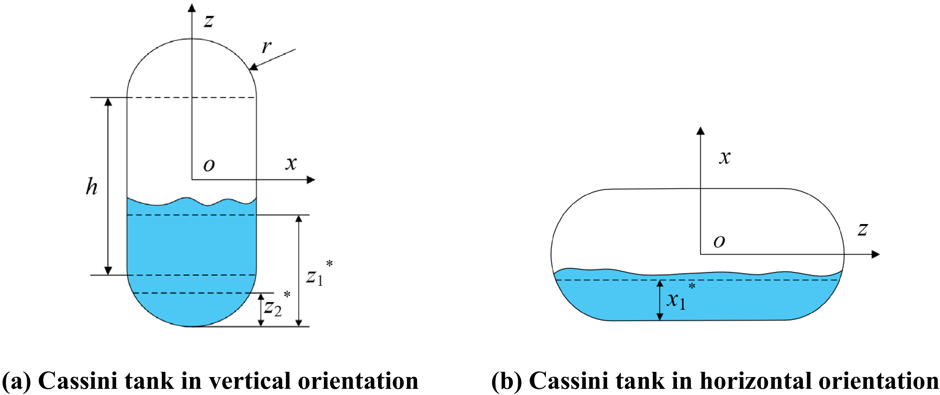

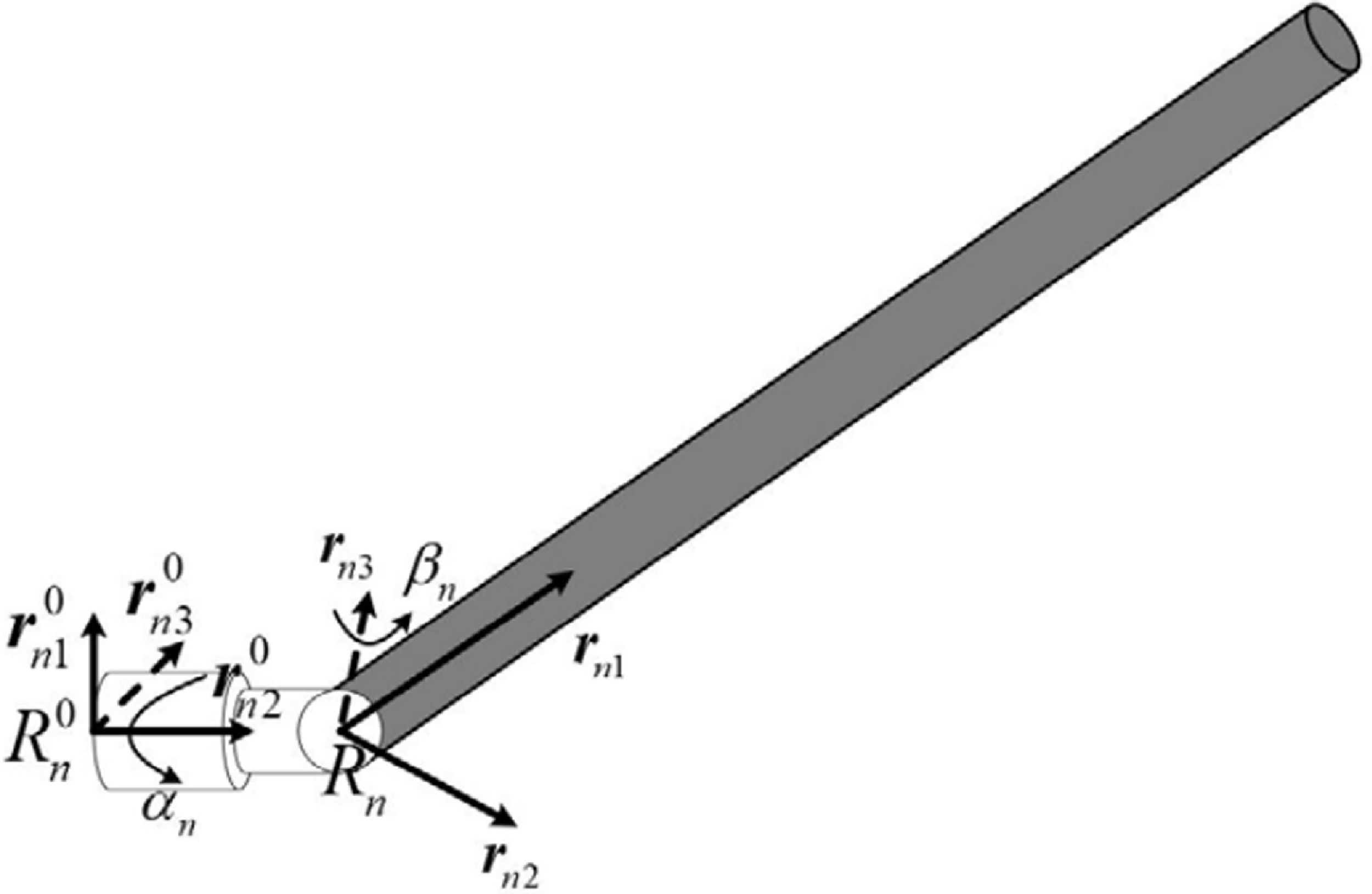
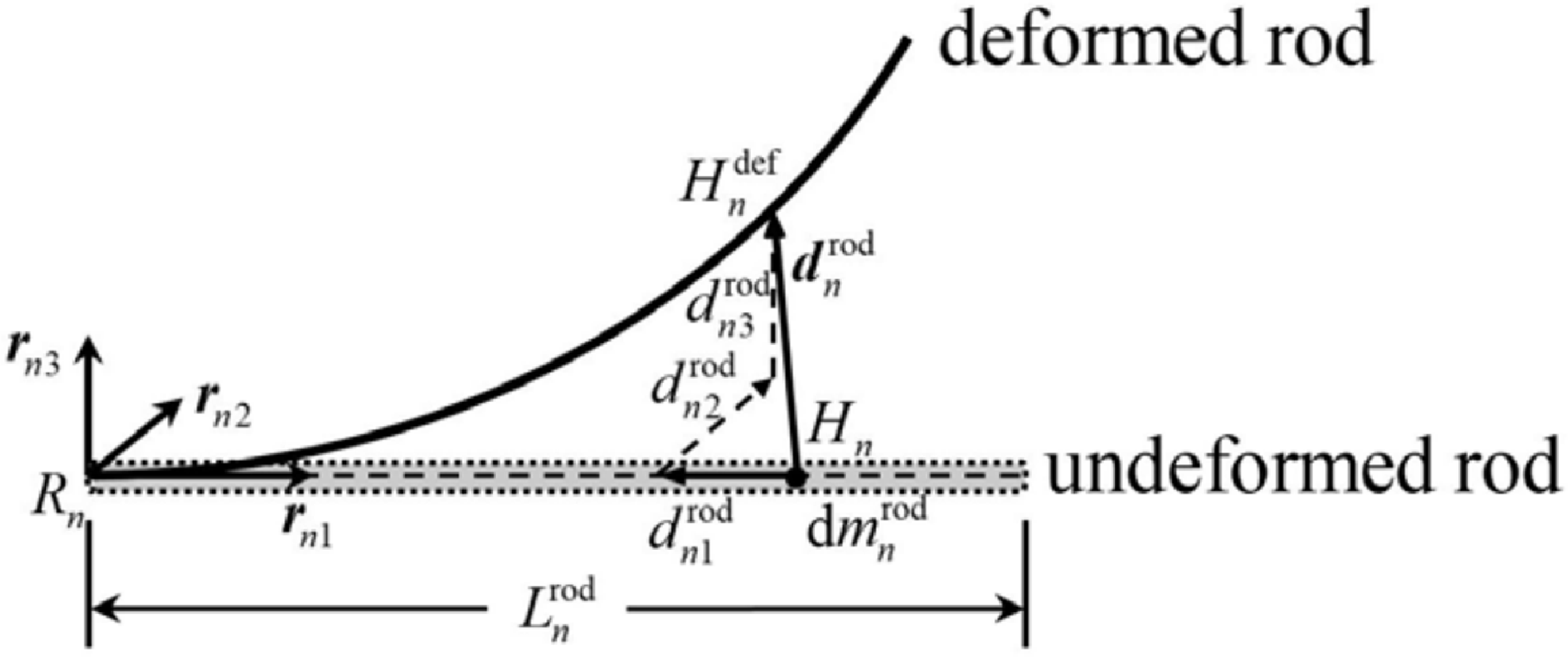
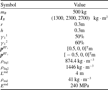
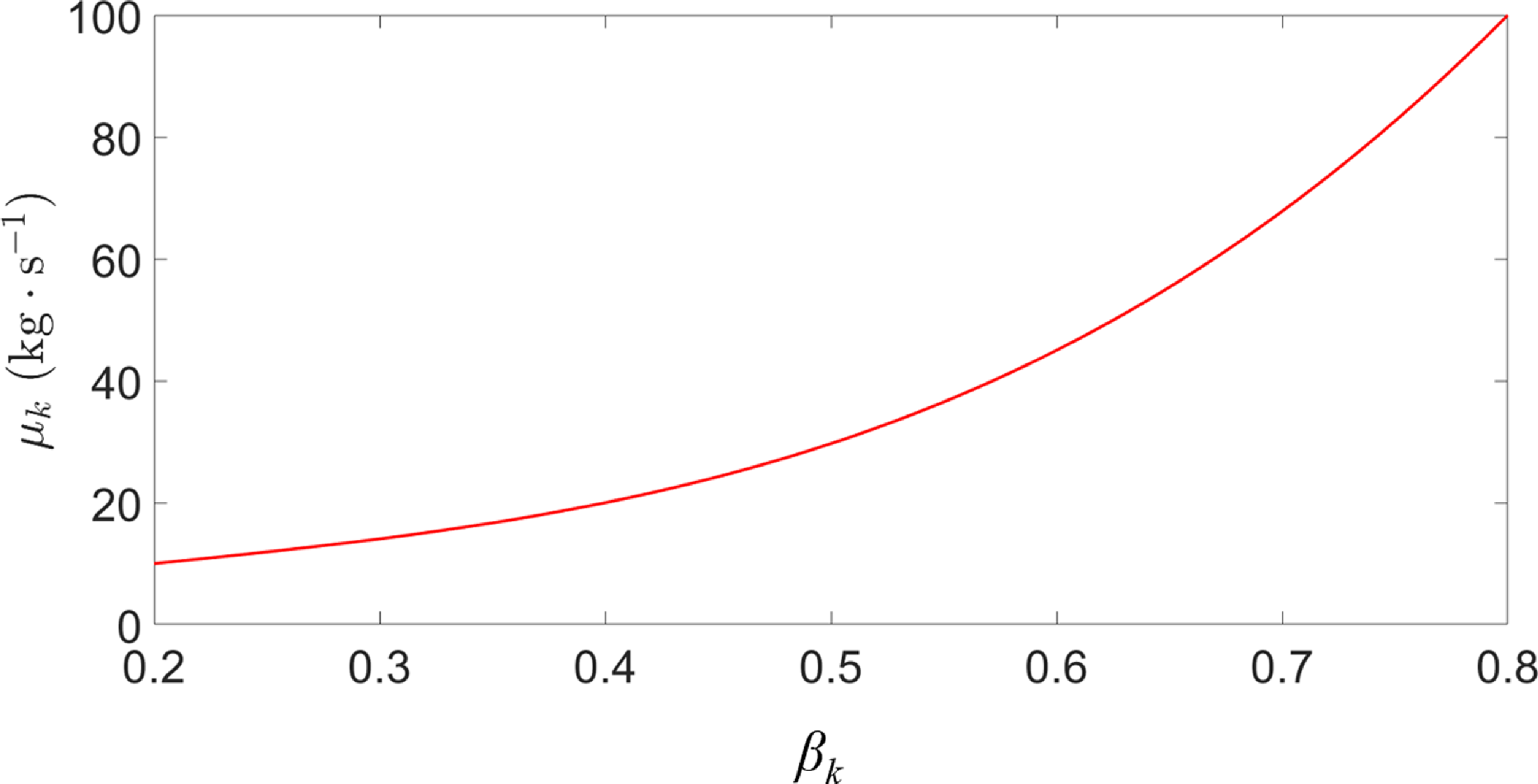
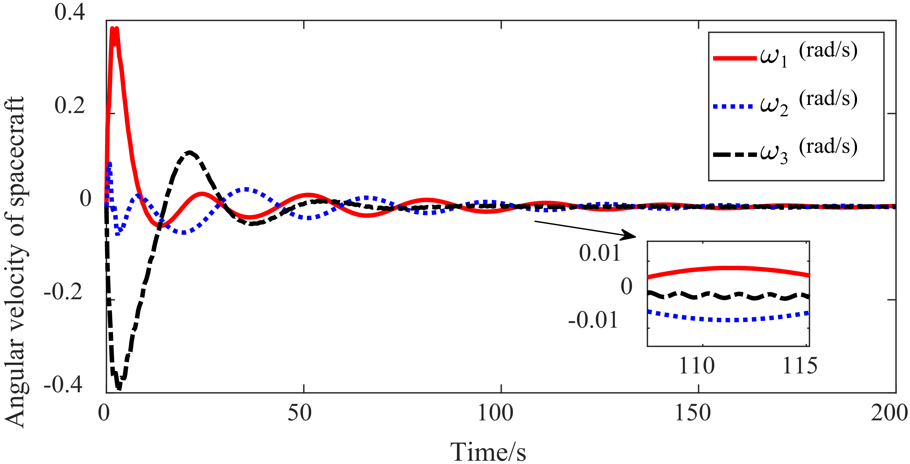

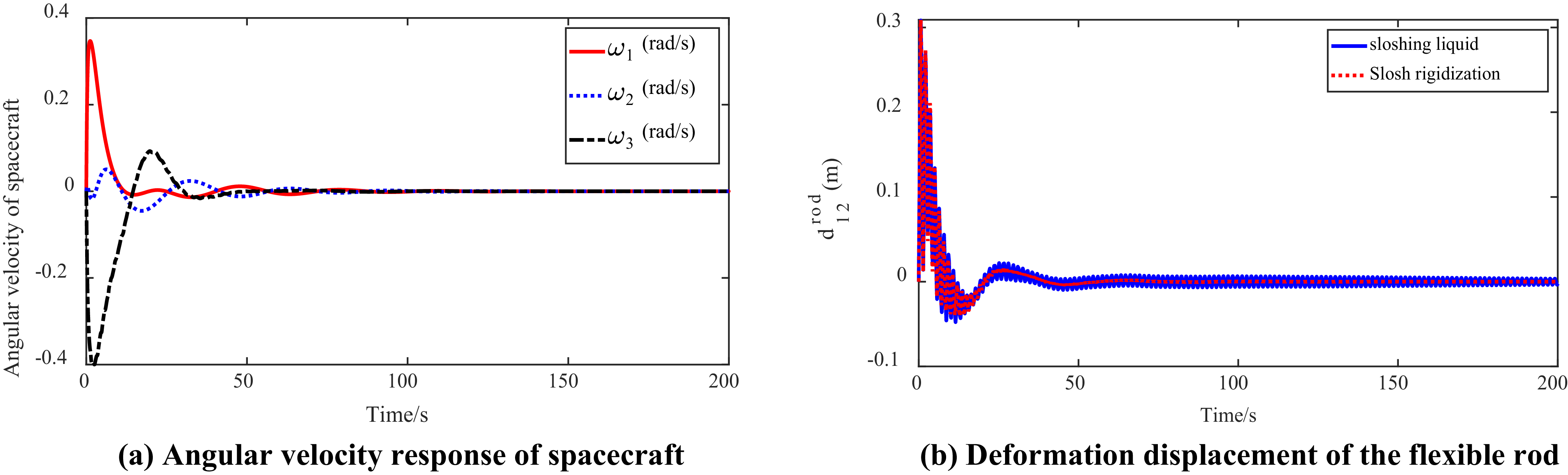
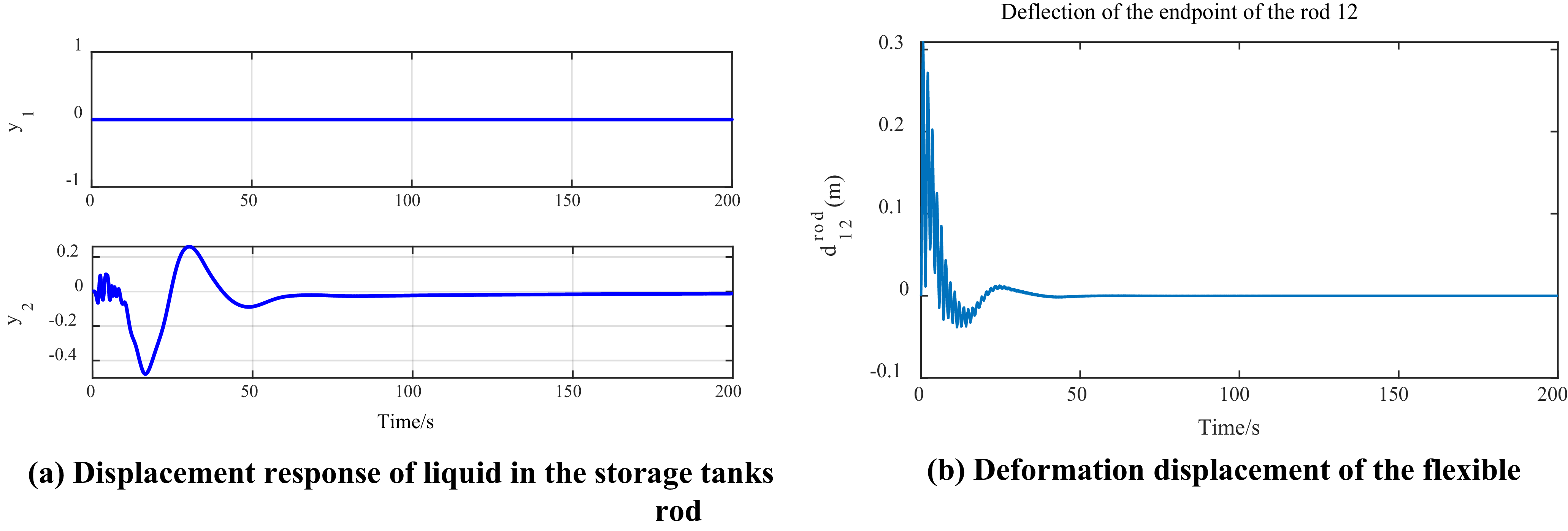
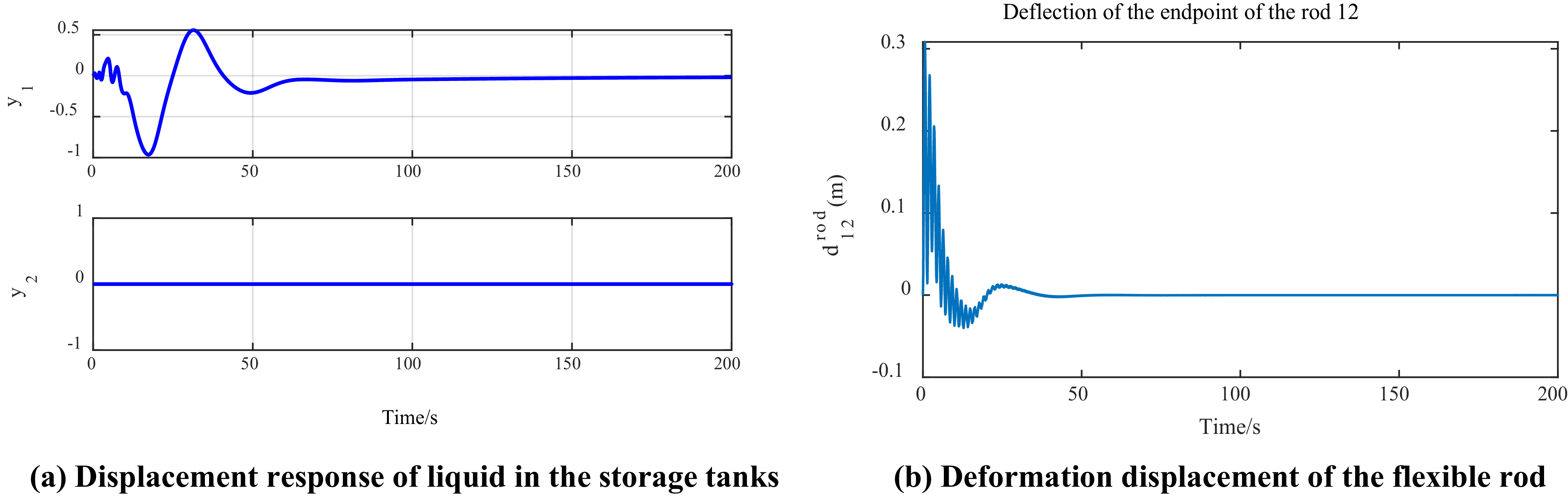

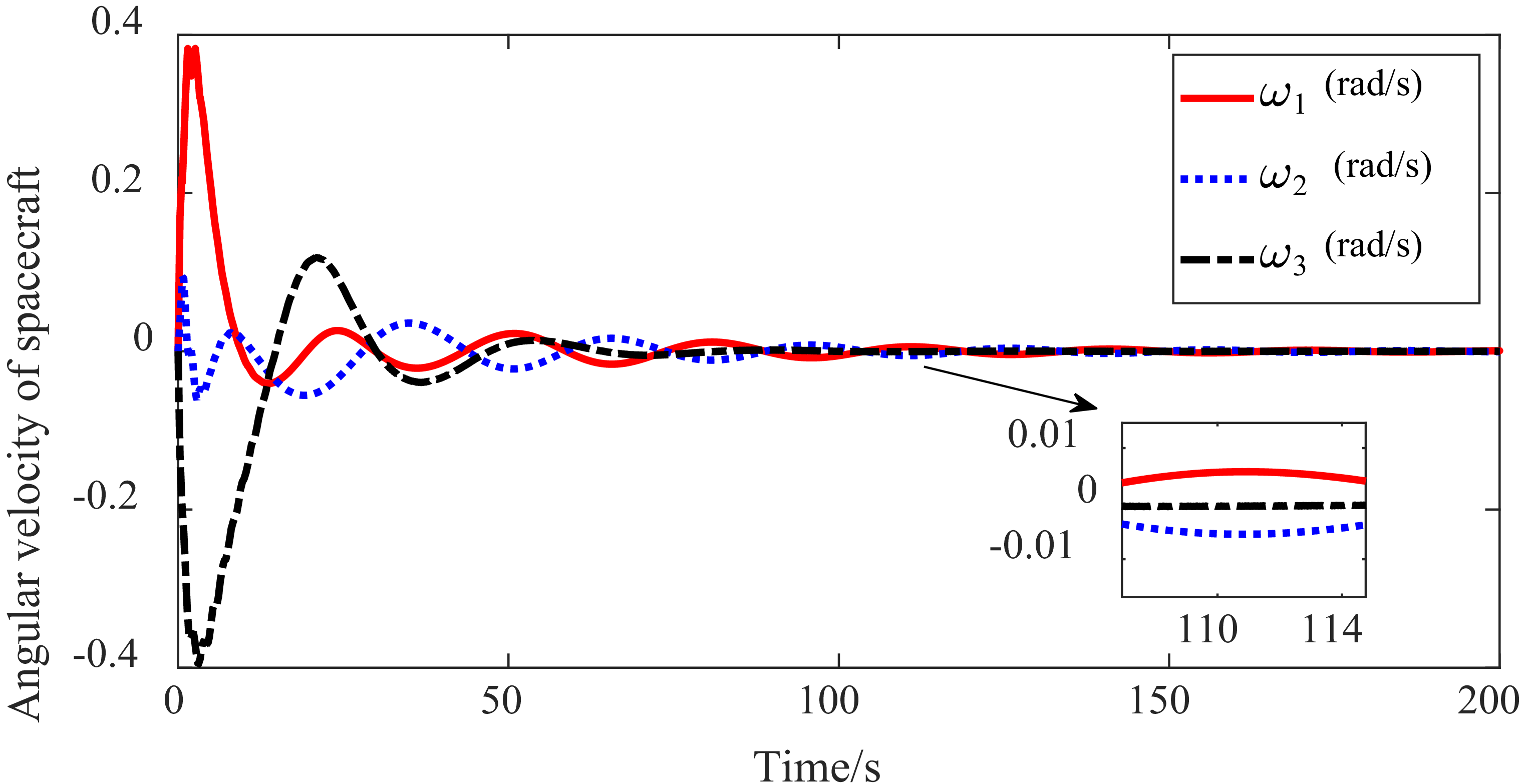
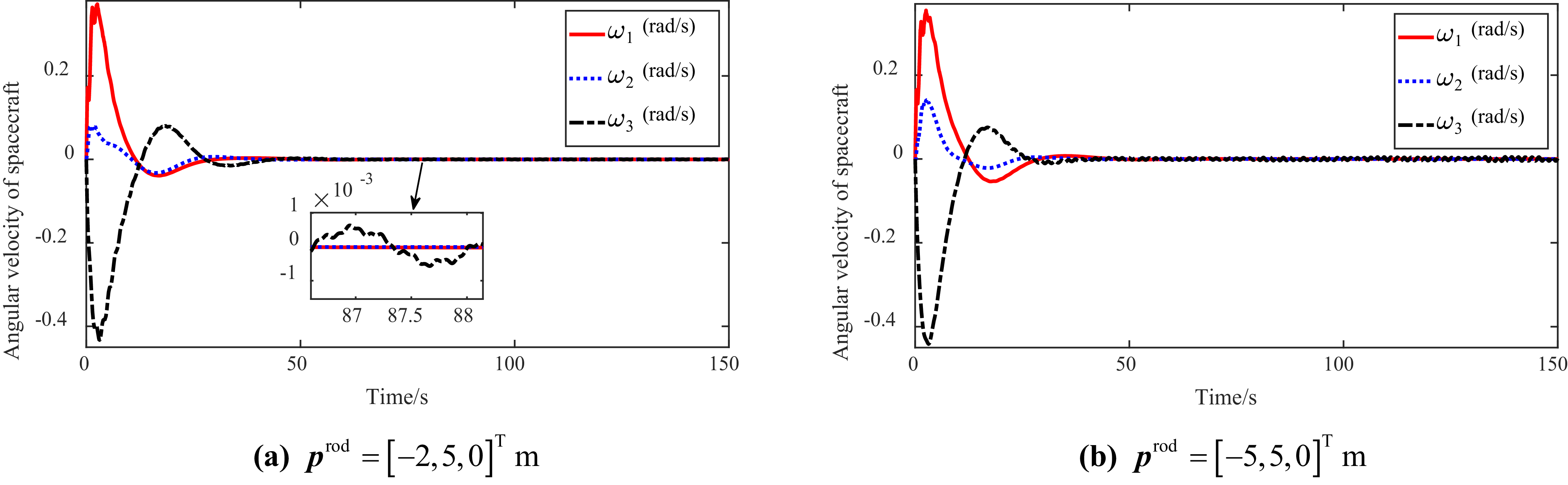

 prod=[−5,5,0]Tm
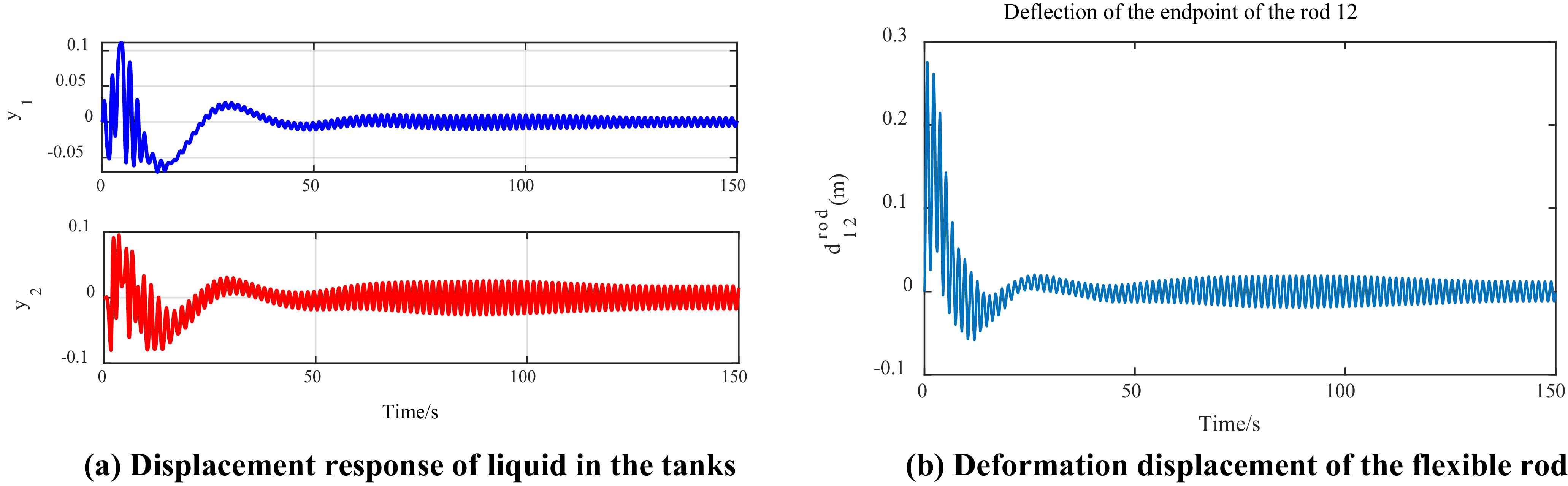
 prod=[0.5,5,0]Tm

 prod=[−1,5,0]Tm
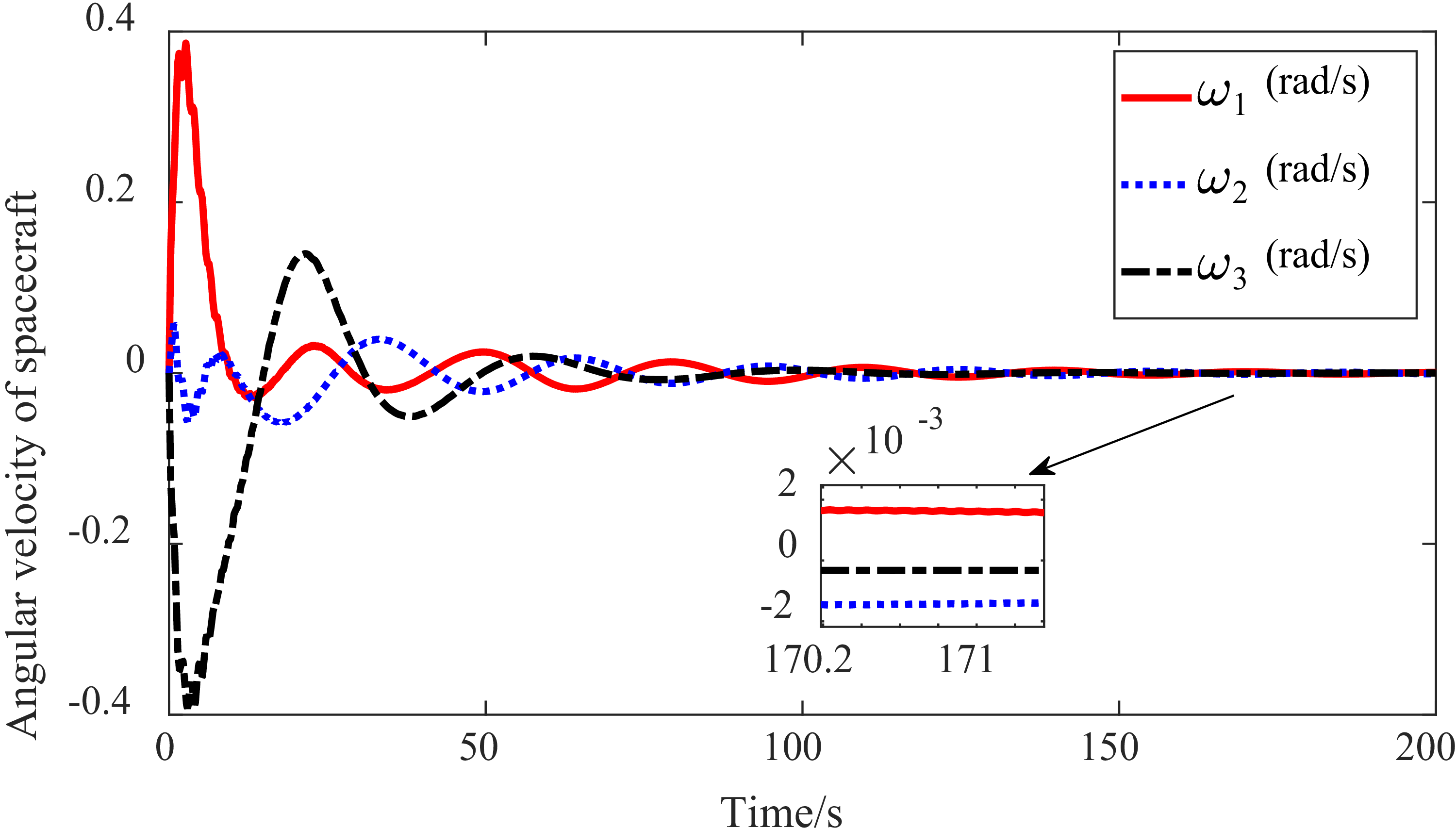
 α˙=β˙=0 rad/s

 α˙=0.01π rad/s,β˙=0.03π rad/s

 α˙=0.01π rad/s,β˙=0.04π rad/s


