1 Introduction
An understanding of and prediction of turbulent boundary layer flows at very high Reynolds numbers (
 $Re$
), and in particular the atmospheric boundary layer (ABL) or its oceanic equivalent, are increasingly becoming critical to a wide range of applications including wind and solar energy, aerodynamic design, meteorology, building and urban design, and assessment of climate change impacts and adaptations. These applications all require a level of sophistication and detail in our ability to probe and model the boundary layer (BL) and its interaction with the surface that manifestly exceeds our current capabilities. Previous work in engineering and geophysical fluid dynamics has largely focused on (quasi) steady-state flows; however, in many applications, the forcing varies at time scales that invalidate this assumption. For example, the real-world ABL is often driven by a range of (sub)meso to synoptic scale forcings (5–1000 km systems) that can evolve over sufficiently short time scales and result in unsteady turbulence (Fritts & Nastrom Reference Fritts and Nastrom1992; Ohfuchi et al.
Reference Ohfuchi, Nakamura, Yoshioka, Enomoto, Takaya, Peng, Yamane, Nishimura, Kurihara and Ninomiya2004). A similar challenge arises in engineering flows such as in reciprocating pumps. Although in most engineering flows the Coriolis force can be neglected, the unsteady turbulence dynamics will be similar to ABL flows.
The resulting unsteady high-
 $Re$
flows involve long-time (or unsteady mean) and short-time (or turbulent) fluctuations that are continuously interacting. From a kinetic energy perspective, this interaction is between the mean kinetic energy (MKE) and turbulent kinetic energy (TKE) via the shear-production term, which is most often positive, denoting conversion of MKE to TKE. A key question for such flows is whether turbulence, and its interaction with the mean, will be quasi-steady, i.e. whether its statistics at any point in time are equivalent to those that would be generated if the current mean forcing at that same point in time were steady. To answer this question in geophysical flows, one needs to understand how the (sub)meso to synoptic scale variability alters the TKE intensity, production, transport and dissipation in the atmospheric or oceanic BL. This challenge frames the goals of this study. We investigate the dynamics of the neutral unsteady Ekman boundary layer (EBL), in which the pressure-gradient, Coriolis and turbulent friction forces interact but are not necessarily in equilibrium. In such unsteady flows, the quasi-steady-state assumption is applicable if turbulence is ‘locally invariant in time’ (self-preserved), i.e. if the largest turbulent eddies are in statistical quasi-equilibrium with the mean flow (and if the smaller eddies are in a quasi-equilibrium with the larger ones, but this is a weaker constraint). However, this is a sufficient but not a necessary condition: while quasi-equilibrium could be expected to fail when the flow is modulated by more than one characteristic time scale (which is the case in our unsteady Ekman flows), this does not necessarily preclude self-preservation or the formulation of similarity laws (Tennekes & Lumley Reference Tennekes and Lumley1972). Therefore, in unsteady conditions, similarity laws analogous to the ones used under a quasi-steady-state could be applicable (perhaps with some modifications).
Various experimental measurements and visualizations have studied oscillatory flows where such conditions might arise (Jensen, Sumer & Fredsoe Reference Jensen, Sumer and Fredsoe1989; Sarpkaya Reference Sarpkaya1993; Lodahl, Sumer & Fredsøe Reference Lodahl, Sumer and Fredsøe1998). Harun et al. (Reference Harun, Monty, Mathis and Marusic2013) investigated the pressure-gradient effect on the large-scale structures of a turbulent BL and indicated that turbulence production results from a combination of the mean shear and large-scale activity that leads to a rise in turbulence intensity. Moreover, the modulation of the small scales by the large scales of motion was found to be influenced by the pressure-gradient values. Hino et al. (Reference Hino, Kashiwayanagi, Nakayama and Hara1983) examined an oscillatory turbulent flow in a rectangular duct and showed that in the accelerating phase turbulence cannot develop, while the onset of flow deceleration allows turbulence to grow rapidly and TKE production becomes very high during this phase (this can be linked to the influence of positive and negative pressure gradients on turbulent BLs). They also reported that the coherent turbulent structures develop within a short time in both oscillatory and steady-state turbulence, even though their statistics differ significantly. The velocity profiles in their experiments depart from the log-law in the acceleration period, while this law is more applicable in the deceleration phase. Since the turbulence time scale is typically shorter than the forcing and mean oscillation scales in many flows, turbulence has the capacity to rapidly adapt to changes in the imposed pressure gradient. However, these experimental studies indicate that this adaptation is not always sufficiently rapid to produce quasi-equilibrium when the variation of the forcing is fast and its time scale is comparable to the turbulence time scale. Mankbadi & Liu (Reference Mankbadi and Liu1992) proposed an unsteady model based on rapid distortion theory that captures some of the flow dynamics in the ‘non-quasi-steady’ forcing frequency range, but their model fails when the changes in the mean are slower and approach quasi-steady-state.
Many research efforts have also examined unsteady BLs using numerical simulations. For instance, Spalart & Baldwin (Reference Spalart and Baldwin1990) studied a sinusoidal oscillating BL with the help of direct numerical simulations (DNS) for intermittent turbulent regimes (at a bulk
 $Re=1000$
). The large-eddy simulation (LES) technique has also been employed previously to simulate unsteady oscillatory turbulent flows (Hsu, Lu & Kwan Reference Hsu, Lu and Kwan2000; Lohmann et al.
Reference Lohmann, Fredsøe, Sumer and Christensen2006; Salon, Armenio & Crise Reference Salon, Armenio and Crise2007). Furthermore, LES has been adopted in studies of freely decaying homogeneous isotropic turbulence, with satisfactory results even under coarse resolutions (Chollet & Lesieur Reference Chollet and Lesieur1981). Scotti & Piomelli (Reference Scotti and Piomelli2001) studied the flow in a turbulent channel under transient pressure gradient with LES and found that high-frequency oscillations were damped before reaching the logarithmic layer. In addition, the density and distribution of coherent structures were different from steady flows, and dependent on the phase of the driving periodic force. Using LES, Gayen, Sarkar & Taylor (Reference Gayen, Sarkar and Taylor2010) documented that the mean velocity in oscillatory BLs exhibits an overshoot with respect to the prevailing free-stream current, which is due to the asymmetric dependence of the Reynolds stress gradient on the tidal phase, and is related to the lack of equilibrium between the mean and turbulence (the latter is known to result in global backscatter, i.e. the conversion of TKE to MKE, as illustrated for example in Bou-Zeid et al. (Reference Bou-Zeid, Overney, Rogers and Parlange2009)). Gayen et al. (Reference Gayen, Sarkar and Taylor2010) also showed that there is a time lag between the maximum TKE magnitude, production and dissipation with respect to the peak external velocity. The TKE budget terms were also examined in a three-dimensional shear-driven turbulent BL generated by moving a section of the wall in the transverse direction by Kannepalli & Piomelli (Reference Kannepalli and Piomelli2000); their results suggested a significant reduction of the TKE after imposing the transverse motion due to disruption of streaky structures and the reduction in the production term.
The large majority of these previous studies, however, did not systematically vary the forcing time scale relative to the inertial and turbulent time scales, and, more importantly, were conducted under the assumption of a very large Rossby number (
 $Ro=\text{inertial force}/\text{Coriolis force}$
), i.e. neglecting the Coriolis force. Therefore, the applicability of their findings to geophysical BLs is questionable. Momen & Bou-Zeid (Reference Momen and Bou-Zeid2016) demonstrated that the presence of the Coriolis force significantly alters the response of the mean flow to temporal changes in the forcing, and as such is expected to also impact the unsteady mean–turbulence dynamics. In particular, the Coriolis force introduces a new inertial EBL time scale (
 $\unicode[STIX]{x1D70F}_{EBL}$
) which will govern the response of the mean flow and which, in conjunction with the pressure-gradient forcing time scale (
 $\unicode[STIX]{x1D70F}_{f}$
) and the turbulence characteristic time scale (
 $\unicode[STIX]{x1D70F}_{t}$
), will modulate the response of both the mean and turbulence to changes in forcing.
This paper aims to bridge this gap and investigate mean–turbulence interactions in an unsteady Ekman flow. Specifically, we aim to answer the following questions.
-
(1) How do the mean and turbulence respond to different forcing time scales, relative to the inertial and turbulence time scales (i.e. under different values of
 $\unicode[STIX]{x1D70F}_{f}/\unicode[STIX]{x1D70F}_{EBL}$
and
$\unicode[STIX]{x1D70F}_{f}/\unicode[STIX]{x1D70F}_{t}$
)?
-
(2) When will the quasi-equilibrium assumption fail, and what are the implications for the mean velocity and turbulence dynamics?
-
(3) Are existing theories, such as the log-law, still valid in unsteady regimes?


Here, we focus on the neutral EBLs, which can occur in nature (see, e.g., measurements of Sugita & Brutsaert Reference Sugita and Brutsaert1990; Mann Reference Mann1994; Högström, Hunt & Smedman Reference Högström, Hunt and Smedman2002), particularly on cloudy days, near sunset or sunrise, and in oceanic flows. We should note that turbulence in the real-world atmospheric or oceanic BLs is often influenced by other unsteady processes (Moeng Reference Moeng1986), and by steady or unsteady boundary heat fluxes as well (surface heating/cooling or cloud top cooling). Such fluxes result in buoyant forces which are another important source of variability that influences the dynamics; however, their impact adds a layer of complexity that is difficult to disentangle without first fully understanding the neutral case. Hence, this is being addressed in a separate paper, and here we intend to first study the interaction of the Coriolis, friction and unsteady pressure-gradient forces, and their implications on the TKE budget, under strictly neutral flows.
In the following section, the numerical details are described and the simulations are introduced. In § 3, the TKE budget time series and vertical profiles in a steady-state EBL are presented as a basis for later comparison with unsteady simulations. Section 4 examines the mean and turbulence response to unsteady forcing (questions 1 and 2). In § 5, the validity of the log-law in various unsteady cases is investigated (question 3), and, in § 6, the implications of unsteady forcing on turbulence closure are investigated using a model based on the mixing-length concept and mean flow variables (question 2). The conclusions are given in § 7.
2 Large-eddy simulations
2.1 Numerical simulations set-up
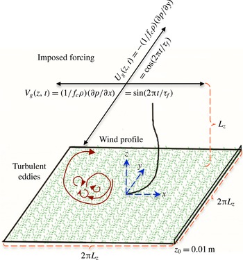
To study mean–turbulence interactions, we employ the LES technique, which resolves the large scales of motion and parameterizes eddies smaller than the filter size. In the code, the mean pressure gradient is represented as an equivalent horizontal geostrophic wind vector with components
 $U_{g}$
and
 $V_{g}$
, as shown in figure 1. All of the results are normalized by the maximum magnitude of the geostrophic wind vector, defined as
 $G=8~\text{m}~\text{s}^{-1}$
, and the BL depth
 $z_{i}$
(
 ${\approx}1000$
m in our simulations). The molecular terms are ignored due to the very high
 $Re$
regime assumption. This also requires the use of a rough wall model, and as such the viscous length scale and Stokes-layer thickness are smaller than the grid–filter size, and are not being resolved in our LES.
The LES code solves the filtered incompressible continuity and Navier–Stokes equations in dimensionless form (rescaled by
 $G$
and
 $z_{i}$
), where a hydrostatic approximation is assumed to hold for the mean flow in the vertical direction (mean vertical pressure gradient and gravity cancel out):
 $$\begin{eqnarray}\displaystyle & \displaystyle \frac{\unicode[STIX]{x2202}\tilde{u} _{i}}{\unicode[STIX]{x2202}x_{i}}=0, & \displaystyle\end{eqnarray}$$
 $$\begin{eqnarray}\displaystyle & \displaystyle \frac{\unicode[STIX]{x2202}\tilde{u} _{i}}{\unicode[STIX]{x2202}t}+\tilde{u} _{j}\left(\frac{\unicode[STIX]{x2202}\tilde{u} _{i}}{\unicode[STIX]{x2202}x_{j}}-\frac{\unicode[STIX]{x2202}\tilde{u} _{j}}{\unicode[STIX]{x2202}x_{i}}\right)=-\frac{1}{\unicode[STIX]{x1D70C}}\frac{\unicode[STIX]{x2202}\tilde{p}^{\ast }}{\unicode[STIX]{x2202}x_{i}}-\frac{\unicode[STIX]{x2202}\unicode[STIX]{x1D70F}_{ij}}{\unicode[STIX]{x2202}x_{j}}+f_{c}(U_{g}-\tilde{u} _{1})\unicode[STIX]{x1D6FF}_{i2}-f_{c}(V_{g}-\tilde{u} _{2})\unicode[STIX]{x1D6FF}_{i1}. & \displaystyle\end{eqnarray}$$
The tilde denotes filtering at the grid/filter scale;
 $x_{i}$
is the position vector;
 $\tilde{u} _{i}=(\tilde{u} ,\tilde{v},\tilde{w})=(\tilde{u} _{1},\tilde{u} _{2},\tilde{u} _{3})$
is the resolved velocity vector;
 $\unicode[STIX]{x1D70F}_{ij}$
is the deviatoric part of the subgrid scale (SGS) stress tensor
 $\unicode[STIX]{x1D70E}_{ij}$
;
 $p^{\ast }$
is a modified pressure into which the resolved and SGS TKE are lumped (see § 2.3);
 $f_{c}$
is the Coriolis parameter, the dimensional value of which is taken as
 $1.394\times 10^{-4}$
Hz (corresponding to
 $73^{\circ }$
latitude); and
 $\unicode[STIX]{x1D6FF}_{ij}$
is the Kronecker delta. For all cases except one,
 $\unicode[STIX]{x1D70F}_{ij}$
is parameterized using the Lagrangian scale-dependent dynamic (LASD) Smagorinsky model, which is detailed and validated for neutral flows in Bou-Zeid, Meneveau & Parlange (Reference Bou-Zeid, Meneveau and Parlange2005). The static Smagorinsky model (with an imposed coefficient that is damped near the surface as described by Bou-Zeid et al.
Reference Bou-Zeid, Meneveau and Parlange2005) is used in one of the cases to assess the influence of the SGS closure on the TKE budget computations.
Schematic view of the simulations:
 $t$
is time;
 $\unicode[STIX]{x1D70F}_{f}$
is the period of the variable pressure forcing;
 $\unicode[STIX]{x1D70C}$
is density;
 $f_{c}$
is the Coriolis parameter;
 $z_{0}=0.01$
m is the surface roughness length;
 $L_{z}=1000$
m is the domain height.

The code uses a pseudo-spectral scheme in the horizontal directions to compute derivatives and for test filtering in the dynamic SGS model. A second-order finite-difference scheme is used in the vertical direction, necessitating a staggered grid. Therefore, the vertical velocity
 $w$
in our simulations is computed and stored halfway in between the other variables (
 $u$
,
 $v$
and
 $p$
). This means that
 $w$
grid points begin at the wall and end at the top of the domain at
 $z=L_{z}$
. The other variables are computed on a grid that starts at
 $\text{d}z/2$
above the wall and continues up to
 $L_{z}+\text{d}z/2$
. This implies that some vertical interpolation will be necessary to compute some of the TKE budget terms later. The vertical velocity,
 $w$
, is set to 0 at the surface. The top boundary conditions for the velocity are no stress,
 $\unicode[STIX]{x1D70F}_{i3}=0$
, and an impermeable wall,
 $w=0$
. The boundary conditions for the pressure field at both the top and bottom surfaces are found from consideration of the vertical momentum balance equation across these boundaries, to be consistent with the zero-vertical-velocity condition, yielding
 $\unicode[STIX]{x2202}\tilde{p}^{\ast }/\unicode[STIX]{x2202}x_{3}+\unicode[STIX]{x2202}\unicode[STIX]{x1D70F}_{j3}/\unicode[STIX]{x2202}x_{j}=0$
, i.e. zero net force. We impose the surface shear stresses through a local-similarity theory formulation: the filtered values of the horizontal velocities (at twice the grid scale) are used to compute the stresses through a local log-law to ensure that the average stresses over the wall are close to the classic mean log-law predictions (see Bou-Zeid et al. (Reference Bou-Zeid, Meneveau and Parlange2005) for more details, performance and validation of the wall model used). Time advancement uses the second-order Adams–Bashforth scheme. The code has been validated in spatially variable flows (e.g. Bou-Zeid et al. (Reference Bou-Zeid, Meneveau and Parlange2005); Li, Bou-Zeid & Anderson (Reference Li, Bou-Zeid and Anderson2016)) that impose similar challenges for the SGS model to the temporally variable ones simulated here; as such, no further validation is deemed necessary. The reader is referred to Bou-Zeid et al. (Reference Bou-Zeid, Meneveau and Parlange2005) and Momen & Bou-Zeid (Reference Momen and Bou-Zeid2016) for more details about the code as used in the present simulations.
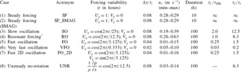
Details of the LES cases. Here,
 $\unicode[STIX]{x0394}t$
is the time-averaging period (2–10 min) and ‘duration’ denotes the dimensional simulation time. The variable forcing, non-dimensionalized by
 $G=8~\text{m}~\text{s}^{-1}$
, has the general form
 $U_{g}=\cos (2\unicode[STIX]{x03C0}t/\unicode[STIX]{x1D70F}_{f});V_{g}=\cos (2\unicode[STIX]{x03C0}t/\unicode[STIX]{x1D70F}_{f})$
. In unsteady cases,
 $u_{\ast }$
is calculated during the last four inertial oscillations,
 $\unicode[STIX]{x1D70F}_{EBL}=12.5$
h, of the simulations. The domain height
 $z_{i}=1000$
m in all of our simulations.

* See § 4 for details on the resonance in these flows.
It should be noted that usually (as long as
 $Ro$
is not too large) the Coriolis frequency characterizes the response time of the mean velocity in geophysical flows with rotation, and thus the natural inertial time scale of the EBL would be
 $\unicode[STIX]{x1D70F}_{EBL}=2\unicode[STIX]{x03C0}/f_{c}\approx 12.5$
h (Tennekes & Lumley Reference Tennekes and Lumley1972). The largest turbulence time scale can also be estimated via
 $\unicode[STIX]{x1D70F}_{t}=z_{i}/u_{\ast }\leqslant 2$
h, where
 $u_{\ast }$
is the friction velocity (
 ${\approx}0.2~\text{m}~\text{s}^{-1}$
). This is the turnover time of the largest eddies which will be approximately as large as the domain height
 $z_{i}$
, but the full spectrum of eddies would be characterized by a range of time scales reaching down to the Kolmogorov time scale (although in LES the smallest scales are not resolved). We will examine the Ekman flow and turbulent BL behaviour for different forcing time periods, relative to the mean and turbulence time scales (i.e. under various values of
 $\unicode[STIX]{x1D70F}_{f}/\unicode[STIX]{x1D70F}_{EBL}$
and
 $\unicode[STIX]{x1D70F}_{f}/\unicode[STIX]{x1D70F}_{t}$
). The time scale that emerges from the non-dimensionalization of the equations (
 $z_{i}/G\approx 125$
s) is not the most relevant to the physics of the present flow (although it is related to the eddy turnover time). Hence, we normalize the simulation time using the inertial time scale of the EBL,
 $\unicode[STIX]{x1D70F}_{EBL}$
, which is constant in all of the cases.
Table 1 describes the eight simulations that we perform, as well as their acronyms which will be used hereafter. The temporal resolution of all cases is 0.15 s (i.e. equivalent to a non-dimensional value of
 $1.2\times 10^{-3}$
when normalized by
 $z_{i}/G$
) and is of the order of the turnover time of the smallest resolved eddies; it is primarily set to maintain numerical stability and satisfy the Courant–Friedrichs–Lewy condition (Madabhushi & Vanka Reference Madabhushi and Vanka1991). The term
 $\unicode[STIX]{x0394}t$
in table 1 stands for the temporal averaging period used in the analyses; some temporal averaging is useful to obtain converged statistics, but its time span must be kept much shorter than any of the relevant time scales of the problem in these unsteady simulations. The Ekman boundary layer thickness (
 $u_{\ast }/f$
) in most of our simulations is less than 1000 m, and thus we resolve this height in such cases. The largest Ekman height occurs in the resonance case, in which it can reach up to 4000 m. However, this height is defined as the height at which the velocity vector is aligned with the geostrophic wind, and its influence on the flow dynamics is not clear (in the real ABL, for example, an inversion could prevent mixing up to that height). To verify whether the domain should extend up to the maximum
 $u_{\ast }/f$
, we conducted another LES of the resonance case with a doubled domain height (
 $L_{z}=2000$
m), while maintaining the same resolution by doubling the number of vertical grid points. The results indicated that the differences between the two simulations were not significant, and therefore our basic domain height of 1000 m is sufficient. Furthermore, since in our simulations the imposed pressure gradients are unsteady, the friction velocity will be time-dependent, and thus
 $u_{\ast }/f$
will also vary in time and with the exerted forcing (see table 1). For instance, this length scale varies between 200 and 700 m in the last two inertial oscillations of the fast and very fast oscillation cases. Therefore, the
 $L_{z}$
, which sets the upper limit on the size of turbulent eddies, is preferred over the
 $u_{\ast }/f$
for normalization of the height, and we set it to 1000 m in all of our simulations.
All of the simulations were performed on a
 $128^{3}$
grid cell numerical mesh. Thus, the vertical spatial resolution of the domain was 1000/128 m and the horizontal resolutions were
 $2\unicode[STIX]{x03C0}\times 1000/128$
m. To test for grid convergence, we also ran some of our simulations (RO and VFO) with a higher resolution (
 $256^{3}$
), and the results obtained were similar to the basic
 $128^{3}$
resolution (not shown); therefore, the educed dynamics and conclusions are not influenced by the numerical set-up.
The first two cases in table 1 are to elucidate the baseline steady-state time variations of the (
 $x$
–
 $y$
) planar-averaged TKE budget and to depict the resolved TKE profiles. We also use them to assess the quality of the SGS modelling and how it influences the closure of the TKE budget. Cases 3–6 are performed to study the dynamics of the mean and turbulence with different forcing variability time scales, from slow to very fast. The forcing magnitude changes in these cases (3–6); its direction, however, remains always aligned along
 $y$
(inducing a geostrophic wind along
 $x$
). In case 7, on the other hand, the pressure-gradient magnitude is fixed but its orientation rotates in time (i.e. the pressure is varying with time in both the
 $x$
- and
 $y$
-directions). The last case is with an unsteady mean pressure forcing but without a Coriolis force (i.e.
 $f_{c}=0$
); we ran it to investigate the influence of (lack of) rotation on the mean and turbulence response. The long simulations are primarily designed to understand the underlying dynamics of the Ekman flows (ensure independence from initial conditions and reproducibility of the statistics over multiple cycles). Although the forcing conditions are only expected to persist in nature for shorter periods (
 ${\sim}$
h), their dynamics can also be investigated from our cases. Such extended periodic forcings are not uncommon in engineering applications (e.g. the UNR case, which has a similar TKE budget dynamics to the other cases with Coriolis, as we show later).
2.2 Large-eddy simulation initialization
A 50 h
 $64^{3}$
node steady simulation is performed to initiate the spin-up. Then, the outputs are linearly interpolated into the
 $128^{3}$
node domain and used as initial values for cases 1 and 2. The rest of the simulations (except UNR) use the final output of case 1 as their initial condition. A similar approach is used for initializing the UNR case, starting from an independent 50 h
 $64^{3}$
node simulation.
2.3 Resolved TKE equation
The pressure field that is computed in our incompressible LES code is not a thermodynamic variable, but rather a dynamic pressure that is modified to include the resolved and SGS TKE components that act normal to a surface (like pressure):
 $$\begin{eqnarray}p\ast =p+{\textstyle \frac{1}{2}}\unicode[STIX]{x1D70C}(u_{j}^{2})+{\textstyle \frac{1}{3}}\unicode[STIX]{x1D70C}\unicode[STIX]{x1D70E}_{kk}.\end{eqnarray}$$
This is done to improve the conservation of resolved energy and to allow the modelling of the deviatoric part of the SGS stress only. If we substitute this pressure expression into (2.2), and apply the Reynolds decomposition and averaging, the conventional forms of the mean kinetic energy
 $\overline{E}=\overline{u}_{i}\overline{u}_{i}/2$
and the resolved turbulent kinetic energy
 $\overline{e}=\overline{u_{i}^{\prime }u_{i}^{\prime }}/2$
arise:
 $$\begin{eqnarray}\displaystyle \frac{\unicode[STIX]{x2202}\overline{E}}{\unicode[STIX]{x2202}t}+\overline{u_{j}}\frac{\unicode[STIX]{x2202}\overline{E}}{\unicode[STIX]{x2202}x_{j}} & = & \displaystyle \overline{u_{i}^{\prime }u_{j}^{\prime }}\frac{\unicode[STIX]{x2202}\overline{u_{i}}}{\unicode[STIX]{x2202}x_{j}}-\frac{(\unicode[STIX]{x1D6FF}_{i1}+\unicode[STIX]{x1D6FF}_{i2})}{\unicode[STIX]{x1D70C}}\frac{\unicode[STIX]{x2202}\overline{u_{i}}\,\overline{p}}{\unicode[STIX]{x2202}x_{i}}-\frac{\unicode[STIX]{x2202}\overline{u_{i}}\overline{u_{i}^{\prime }u_{j}^{\prime }}}{\unicode[STIX]{x2202}x_{j}}\nonumber\\ \displaystyle & & \displaystyle -\,\frac{1}{3}\frac{\unicode[STIX]{x2202}\overline{u_{i}}\,\overline{\unicode[STIX]{x1D70E}_{kk}}}{\unicode[STIX]{x2202}x_{i}}-\frac{\unicode[STIX]{x2202}\overline{u_{i}}\,\overline{\unicode[STIX]{x1D70F}_{ij}}}{\unicode[STIX]{x2202}x_{j}}+\overline{\unicode[STIX]{x1D70F}_{ij}}\overline{S_{ij}}+f_{c}\unicode[STIX]{x1D716}_{ij3}\overline{u_{i}}\,\overline{u_{j}},\end{eqnarray}$$
 $$\begin{eqnarray}\displaystyle \frac{\unicode[STIX]{x2202}\overline{e}}{\unicode[STIX]{x2202}t}+\overline{u_{j}}\frac{\unicode[STIX]{x2202}\overline{e}}{\unicode[STIX]{x2202}x_{j}} & = & \displaystyle -\overline{u_{i}^{\prime }u_{j}^{\prime }}\frac{\unicode[STIX]{x2202}\overline{u_{i}}}{\unicode[STIX]{x2202}x_{j}}-\frac{1}{\unicode[STIX]{x1D70C}}\frac{\unicode[STIX]{x2202}\overline{u_{i}^{\prime }p^{\prime }}}{\unicode[STIX]{x2202}x_{i}}-\frac{1}{3}\frac{\unicode[STIX]{x2202}\overline{u_{i}^{\prime }\unicode[STIX]{x1D70E}_{kk}^{\prime }}}{\unicode[STIX]{x2202}x_{i}}-\frac{\unicode[STIX]{x2202}\overline{u_{i}^{\prime }e}}{\unicode[STIX]{x2202}x_{i}}-\overline{\frac{\unicode[STIX]{x2202}u_{i}^{\prime }\unicode[STIX]{x1D70F}_{ij}^{\prime }}{\unicode[STIX]{x2202}x_{j}}}+\overline{\unicode[STIX]{x1D70F}_{ij}^{\prime }S_{ij}^{\prime }},\end{eqnarray}$$
where the overbar denotes the ensemble average and the prime denotes the turbulent fluctuation from the ensemble average. The hydrostatic approximation for the mean allows us to omit the gravity and
 $\unicode[STIX]{x2202}\overline{p}/\unicode[STIX]{x2202}z$
terms in (2.4) (hence only the
 $\unicode[STIX]{x1D6FF}_{i1}+\unicode[STIX]{x1D6FF}_{i2}$
in the pressure term). It should be noted that all
 $u_{i}$
,
 $p$
and
 $S_{ij}$
in the above equations are the resolved components, and we will omit the tildes for notational simplicity. Since the SGS kinetic energy
 $\unicode[STIX]{x1D70E}_{kk}$
would require a model that is distinct from our model for the deviatoric part
 $\unicode[STIX]{x1D70F}_{ij}$
, and since it makes a small contribution to the terms in (2.4) and (2.5) relative to its resolved counterpart away the wall (this is verified using a simple model for
 $\unicode[STIX]{x1D70E}_{kk}$
in appendix A), we neglect the terms that include this component rather than risk introducing modelling errors that could be of the same order as the magnitude of the terms involving
 $\unicode[STIX]{x1D70E}_{kk}$
. Furthermore, in our TKE budget calculations, we can safely assume no subsidence,
 $\overline{w}=0$
, and periodic statistical homogeneity in both horizontal directions; hence, equations (2.4) and (2.5) reduce to
 $$\begin{eqnarray}\displaystyle \frac{\unicode[STIX]{x2202}\overline{E}}{\unicode[STIX]{x2202}t} & = & \displaystyle \overline{u^{\prime }w^{\prime }}\frac{\unicode[STIX]{x2202}\overline{u}}{\unicode[STIX]{x2202}z}+\overline{v^{\prime }w^{\prime }}\frac{\unicode[STIX]{x2202}\overline{v}}{\unicode[STIX]{x2202}z}-\frac{(\unicode[STIX]{x1D6FF}_{i1}+\unicode[STIX]{x1D6FF}_{i2})}{\unicode[STIX]{x1D70C}}\overline{u_{i}}\frac{\unicode[STIX]{x2202}\overline{p}}{\unicode[STIX]{x2202}x_{i}}-\frac{\unicode[STIX]{x2202}\overline{u_{i}}\overline{u_{i}^{\prime }w^{\prime }}}{\unicode[STIX]{x2202}z}\nonumber\\ \displaystyle & & \displaystyle -\,\frac{\unicode[STIX]{x2202}\overline{u_{i}}\,\overline{\unicode[STIX]{x1D70F}_{i3}}}{\unicode[STIX]{x2202}z}+\overline{\unicode[STIX]{x1D70F}_{ij}}\overline{S_{ij}}+f_{c}\unicode[STIX]{x1D716}_{ij3}\overline{u_{i}}\,\overline{u_{j}},\end{eqnarray}$$
 $$\begin{eqnarray}\displaystyle \frac{\unicode[STIX]{x2202}\overline{e}}{\unicode[STIX]{x2202}t} & = & \displaystyle -\overline{u^{\prime }w^{\prime }}\frac{\unicode[STIX]{x2202}\overline{u}}{\unicode[STIX]{x2202}z}-\overline{v^{\prime }w^{\prime }}\frac{\unicode[STIX]{x2202}\overline{v}}{\unicode[STIX]{x2202}z}-\frac{1}{\unicode[STIX]{x1D70C}}\frac{\unicode[STIX]{x2202}\overline{w^{\prime }p^{\prime }}}{\unicode[STIX]{x2202}z}-\frac{\unicode[STIX]{x2202}\overline{w^{\prime }e}}{\unicode[STIX]{x2202}z}-\overline{\frac{\unicode[STIX]{x2202}u_{i}^{\prime }\unicode[STIX]{x1D70F}_{i3}^{\prime }}{\unicode[STIX]{x2202}z}}+\overline{\unicode[STIX]{x1D70F}_{ij}^{\prime }S_{ij}^{\prime }}.\end{eqnarray}$$
We compute the TKE budget in terms of the resolved variables and define the following expressions for the terms in (2.6) and (2.7) for the rest of the paper as follows:
 $$\begin{eqnarray}\displaystyle \left.\begin{array}{@{}c@{}}\displaystyle P\equiv -\overline{u^{\prime }w^{\prime }}\frac{\unicode[STIX]{x2202}\overline{u}}{\unicode[STIX]{x2202}z}-\overline{v^{\prime }w^{\prime }}\frac{\unicode[STIX]{x2202}\overline{v}}{\unicode[STIX]{x2202}z}=\left(\overline{u}\,\overline{w}-\overline{uw}\right)\frac{\unicode[STIX]{x2202}\overline{u}}{\unicode[STIX]{x2202}z}+\left(\overline{v}\,\overline{w}-\overline{vw}\right)\frac{\unicode[STIX]{x2202}\overline{v}}{\unicode[STIX]{x2202}z},\\ \displaystyle PT\equiv -\frac{1}{\unicode[STIX]{x1D70C}}\frac{\unicode[STIX]{x2202}\overline{w^{\prime }p^{\prime }}}{\unicode[STIX]{x2202}z}=\frac{1}{\unicode[STIX]{x1D70C}}\frac{\unicode[STIX]{x2202}}{\unicode[STIX]{x2202}z}\left(\overline{w}\,\overline{p}-\overline{wp}\right),\\ \displaystyle RT\equiv -\frac{\unicode[STIX]{x2202}\overline{w^{\prime }e}}{\unicode[STIX]{x2202}z}=-\frac{1}{2}\frac{\unicode[STIX]{x2202}}{\unicode[STIX]{x2202}z}\left(\overline{u^{2}w}-2\overline{u}\,\overline{uw}+\overline{v^{2}w}-2\overline{v}\,\overline{vw}+\overline{w^{3}}\right),\\ \displaystyle ST\equiv -\overline{\frac{\unicode[STIX]{x2202}u_{i}^{\prime }\unicode[STIX]{x1D70F}_{i3}^{\prime }}{\unicode[STIX]{x2202}w}}=-\frac{\unicode[STIX]{x2202}}{\unicode[STIX]{x2202}z}\left(\overline{u\unicode[STIX]{x1D70F}_{13}}-\overline{u}\,\overline{\unicode[STIX]{x1D70F}_{13}}+\overline{v\unicode[STIX]{x1D70F}_{23}}-\overline{v}\,\overline{\unicode[STIX]{x1D70F}_{23}}+\overline{w\unicode[STIX]{x1D70F}_{33}}\right),\\ T\equiv PT+RT+ST,\\ \displaystyle \unicode[STIX]{x1D716}\equiv \overline{\unicode[STIX]{x1D70F}_{ij}^{\prime }S_{ij}^{\prime }}=\overline{\unicode[STIX]{x1D70F}_{ij}S_{ij}}-\overline{\unicode[STIX]{x1D70F}_{ij}}\overline{S_{ij}},\end{array}\right\} & & \displaystyle\end{eqnarray}$$
where
 $P$
,
 $PT$
,
 $RT$
,
 $ST$
,
 $T$
and
 $\unicode[STIX]{x1D716}$
are respectively the shear production, pressure transport (correlation), resolved turbulent transport, SGS turbulent transport, total TKE transport and SGS dissipation. Our LES code computes each of these terms by averaging in space and time. To obtain the averaged quantities on the right-hand side of (2.8), first, a spatial average over the horizontal directions is applied to acquire a single instantaneous profile for each term (to define the ensemble average). Then, all of these TKE budget profiles are calculated instantaneously (this involves products and vertical derivatives), and finally the profiles of the budget terms are averaged in time over the short
 $\unicode[STIX]{x0394}t$
intervals indicated in table 1. Time averaging before computing the terms in (2.8) was found to cause significant errors in this unsteady framework due to the time variation of the parameters that need to be Reynolds-averaged. Hence, only spatial averaging is used as a surrogate for Reynolds averaging, although the resulting unsteady statistics are then averaged over
 $\unicode[STIX]{x0394}t$
. A similar procedure is applied to produce velocity and other time series.
It should be noted that because of the staggered set-up of the numerical domain, we linearly interpolated all terms from the
 $w$
nodes into
 $u{-}v{-}p$
nodes when needed, and subsequently applied the multiplications and differentiations in (2.8). This could be a source of error in the results, but as the numerical grids become finer this error would be expected to decrease.
3 Turbulent kinetic energy budget in steady-state conditions
The TKE budget is first computed for a steady EBL to understand the magnitude of the variations of its terms in time. Since the unsteady nature of the mean flow prevents us from applying a long-time average, we need to assess the statistical convergence of the results from spatial averaging over an
 $x$
–
 $y$
plane and short-time averaging. Moreover, as one can observe from (2.8), the TKE budget terms are influenced by the SGS model in the LES. The SGS model affects dissipation and SGS transport directly, and other terms indirectly. To illustrate the significance of the SGS model, two steady simulations are performed. Case 1 is a 10 h steady LES with the LASD SGS model, while case 2 is the same simulation but with the static Smagorinsky model.
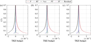
Turbulent kinetic energy budget profiles, normalized using
 $G$
and
 $z_{i}$
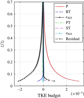
, for case 1 with spatial averaging (a), case 1 with both spatial and temporal averaging (b), and case 2 with both spatial and temporal averaging (c).

Figure 2(a) displays case 1, where the perturbations are computed relative to a spatial average (
 $x$
–
 $y$
plane), then the TKE budget terms are computed, and then averaged in both space and time from
 $t=5$
to 5.17 h (i.e. for approximately 10 min; this is the approach described before and that we use for the unsteady simulations with short-time averaging as in table 1). This spatial averaging, however, might not be sufficient to yield a statistically converged ensemble average. Therefore, figure 2(b) exhibits profiles where the perturbations are computed relative to a spatial and (long) temporal average, and then the statistics are further averaged in space (
 $x$
–
 $y$
plane) and time from
 $t=2$
to 9.5 h. It is obvious from this figure that, as expected, time averaging before computing the perturbations improves the statistical convergence, and hence reduces the uncertainty in the calculated terms (reduces the residual). The TKE budget residual, however, remains non-zero, especially near the wall. This is partially related to the need for vertical interpolation. However, since in computations with the exact same code as used in DNS mode (albeit with higher vertical resolution that reduces the interpolation errors) for steady flows the TKE budget closure is nearly perfect (see Shah & Bou-Zeid Reference Shah and Bou-Zeid2014), one can conclude that the lack of closure here is also related to the fact that in LES mode the TKE budget equation is not necessarily balanced. This can also be deduced, for example, by noting that for a given flow state (
 $u$
,
 $v$
,
 $w$
,
 $p$
), the balance of (2.7) depends on the approximate SGS model used for
 $\unicode[STIX]{x1D70F}_{ij}$
. The SGS model is primarily designed to optimize the velocity moments and profiles or to produce the correct wall-shear stress in the case of the wall model, and the SGS dissipation it produces might have errors that preclude the exact closure of the TKE budget. Hence, the residual departure from zero, especially near the wall where the shear production and dissipation are very high, is not surprising (see computations with other LES codes that illustrate the same trends and residuals like Kosovic (Reference Kosovic1997), and also see the lack of the LES TKE budget closure in Kosovic & Curry (Reference Kosovic and Curry2000), Drobinski & Foster (Reference Drobinski and Foster2003) and Catalano & Moeng (Reference Catalano and Moeng2010)). Inclusion of the terms associated with the SGS TKE correction in the pressure transport (using a model for that energy) makes a small difference in the results and does not improve the closure, as illustrated in appendix A.
Furthermore, comparison of figure 2(b) (LASD) and figure 2(c) (static Smagorinsky) confirms that the shape of the TKE budget profiles and the closure are influenced by the choice of the SGS model, although both models do not close the budget. This is more evident in the SGS transport and dissipation terms that are directly impacted by the SGS closure scheme. The SGS transport term is sensitive to time averaging as well (compare a and b). The LASD has lower dissipation values than the static Smagorinsky, and while that produces better energy spectra (Bou-Zeid et al. Reference Bou-Zeid, Meneveau and Parlange2005), it appears to result in larger TKE residuals.
Nevertheless, we will continue to use the LASD model in the rest of the simulations since it yields enhanced mean profiles, velocity moments, and spectra. In addition, dynamic procedures like the one used in the LASD are better suited for cases involving disequilibrium and anisotropic flows, and Lagrangian time integration over flow pathlines is shown to respond quickly to unsteadiness in the mean flow due to its relatively short time scale (Meneveau & Katz Reference Meneveau and Katz2000). In oscillatory BLs, mean velocity profiles and turbulence intensities resulting from dynamic models give better agreement with experimental results than other SGS models, as shown by Radhakrishnan & Piomelli (Reference Radhakrishnan and Piomelli2008). That study also showed that the use of models that do not dissipate excessive amounts of energy is crucial in these flows since such models yield a lower SGS eddy viscosity, which allows the inner layer to adapt faster to the imposed variations. On the other hand, other excessively dissipative models, like Smagorinsky, do not respond quickly enough to the changes in the pressure-gradient field, leading to incorrect velocity profiles. Similar findings in spatially variable flows were also reported in other studies (Kirkil et al. Reference Kirkil, Mirocha, Bou-Zeid, Chow and Kosović2012; Mirocha et al. Reference Mirocha, Kirkil, Bou-Zeid, Chow and Kosović2013). The presence of shear and rotation also affects SGS dissipation, such that a constant scale-invariant Smagorinsky coefficient is not appropriate (Canuto & Cheng Reference Canuto and Cheng1997).
Given that we could not avoid the finite residual in the TKE budget, we will assume that its magnitude characterizes the uncertainty in the computation of the TKE terms. Therefore, we will plot it as error bands in the following figures (the plotted residual is computed for every simulation and at every time separately; this uncertainty should be applied to all of the terms, but we only plot it on the production term to avoid cluttering the plots).
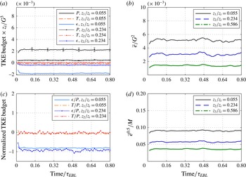
Figure 3 depicts the variability of the TKE budget terms in time for the steady-state case 1, after averaging over an
 $x$
–
 $y$
plane, at three different heights. This moderate variability is related to the lack of full statistical convergence when only spatial averaging is performed. In figure 3(a), the dimensionless TKE budget time series are illustrated, while figure 3(c) depicts the budget terms normalized by the shear production. Although they feature some variations, the rate of the fluctuations of these time series from their mean value is small.
The dimensionless TKE and turbulence intensity (defined as the square root of TKE normalized by the mean wind magnitude
 $M\equiv (\overline{u}^{2}+\overline{v}^{2})^{1/2}$
), shown in figure 3(b,d), also display a constant mean at each height with small variations in time. It should be noted that the rapid changes in the first 30 min of the figures are related to the development of smaller-scale turbulence as the grid is refined from
 $64^{3}$
to
 $128^{3}$
. This confirms that our initialization technique, discussed in § 2.2, equilibrates very fast (
 $0.04\unicode[STIX]{x1D70F}_{EBL}$
on the fine grid) and is very useful since it reduces the computational spin-up time significantly compared with a higher-resolution initialization.
Time series of (a) dimensionless TKE budget terms (with error bands depicting the residual of the TKE budget), (b) dimensionless TKE, (c) TKE budget normalized by the production
 $P$
and (d) turbulence intensity, for case 1.

4 Mean and turbulence response to variable forcing
4.1 Turbulence intensity variations
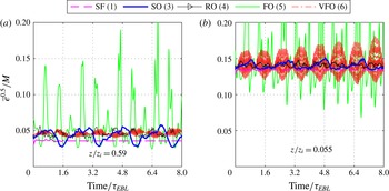
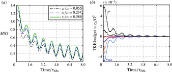
Turbulence typically has a smaller time scale than the mean flow; thus, it is expected that the turbulence intensity (TI) should adjust itself to the variations in the mean very rapidly. That is, turbulence is usually near a quasi-equilibrium state with the mean flow, and TI should remain constant for a given flow. However, if the forcing of the mean varies at time scales commensurate with those of turbulence, the adjustment might not be sufficiently fast. This could result in variations in the turbulence statistics, even the ones normalized by mean variables such as TI. This departure from quasi-equilibrium is illustrated in figure 4 for the varying pressure-gradient simulations: TI fluctuates strongly compared with the steady-state simulation. It should be noted that since the simulation time of the steady case SF is
 $0.8\unicode[STIX]{x1D70F}_{EBL}$
, its averaged value is extrapolated up to
 $t=8.0\unicode[STIX]{x1D70F}_{EBL}$
in the figure for comparison with the longer unsteady runs. Since the forcing is not changing in this case, the variations in TI are expected to remain similar to the simulated 10 h.
Turbulence intensity for five simulations, (a) in the middle of the EBL and (b) near the wall. The peaks of the FO case in (b) rise up to 0.8.

The TI in the slow-oscillation case displays a periodic behaviour in which the magnitude of the oscillations is approximately three quarters of the mean value at
 $z/z_{i}=0.59$
(figure 4
a), despite the fact that the forcing time scale in this case is two times the inertial time scale. If one compares the TI minima and maxima for SO with the mean horizontal velocity
 $M$
in figure 5(a), opposite trends can be observed (as one peaks the other troughs). The very-fast-oscillation case also shows variations in the TI times series (up to 20 % of the mean) at
 $z/z_{i}=0.59$
. However, the strongest time variability occurs in the fast-oscillation FO case (this will be explained in the next subsection).
The
 $M$
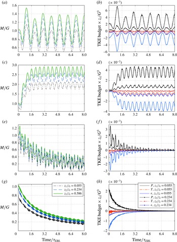
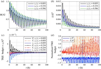
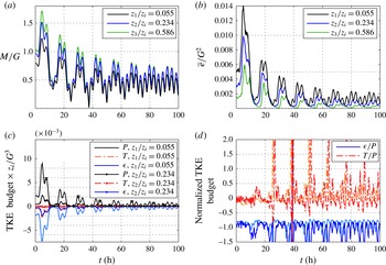
(a,c,e,g) and TKE budget (b,d,f,h) time series for case 3 SO (a,b), 4 RO (c,d), 5 FO (e,f) and 6 VFO (g,h).

Figure 4 also indicates that the TI variations near the surface (
 $z/z_{i}=0.055$
) are lower for the SO, RO and SF cases than near the middle of the domain (
 $z/z_{i}=0.59$
). This is due to the quicker response (smaller effective
 $\unicode[STIX]{x1D70F}_{t}$
) of the smaller eddies near the surface to the imposed variations and their faster equilibration. On the other hand, when the imposed forcing time scale is of the order of or smaller than the turbulence time scale (FO and VFO), the eddies might not find adequate time to respond, and therefore the variations in TI do not decrease as height decreases. Nonetheless, the results suggest that while the FO case depicts strong variability as expected, the VFO case seems not to depart strongly from equilibrium conditions. These high variations in the surface layer emerge when
 $M$
gets close to zero while the TKE, which decays slowly and can also be transported from above, remains high in the EBL.
These simulations imply that the TI is rarely constant in unsteady flows; it changes according to the mean pressure variations even when those variations occur at diurnal time scales (
 ${\sim}24~\text{h}=1~\text{day}$
) two times larger than the inertial period of the EBL in the paper (
 ${\sim}12$
h). As the forcing time scale increases even further, a quasi-steady TI would eventually be expected. These variations could either imply non-equilibrium, or they could be due to the changes in the
 $Ro$
and the effective
 $Re$
of the LES (note that the LES has an effective
 $Re$
imposed by the SGS model and/or the grid resolution, despite the fact that we ignore the molecular terms). We will revisit this point in § 4.4.
4.2 Turbulent kinetic energy budget variations
The unsteady forcing alters the mean and turbulent velocity time series differently, as can be concluded from the TI plots in the previous subsection. We seek to understand how these different responses of the mean and turbulence are modulated by their dynamics and their interaction. To that end, the time series of the dimensionless mean wind velocity at three heights and the dimensionless TKE budget terms at two heights are plotted. Figure 5(a,b) exhibits case SO. One can observe that all of the TKE budget terms, at a given height, peak and trough at the same time. Furthermore, the peaks in the shear production correspond in time to the peaks in
 $M$
, albeit with a small lag relative to the mean wind (see § 6), and a similar behaviour is observed in the troughs. This indicates that the turbulence and mean dynamics are well correlated, although they are not perfectly synchronized.
The next simulation, presented in figure 5(c,d) is the resonant-forcing case (
 $\unicode[STIX]{x1D70F}_{forcing}\approx \unicode[STIX]{x1D70F}_{EBL}$
), which illustrates the increased TKE levels as the mean resonates and increases beyond the geostrophic wind speeds (
 $M/G>1$
, figure 5
c). As detailed in Momen & Bou-Zeid (Reference Momen and Bou-Zeid2016), this can be conceptually explained by considering the damped-oscillator (mass–spring–damper) model for the response of the mean flow in the EBL to a variable forcing. In that paper, we showed that the mean dynamics can be simply represented by two coupled second-order ordinary differential equations (ODEs) for the means of
 $u$
and
 $v$
, like a damped oscillator (underdamped for the EBL). As such, the mean dynamics are characterized by a single natural time scale
 $\unicode[STIX]{x1D70F}_{EBL}$
, and they damp or magnify the magnitude of the forcing (transmissibility ratio) depending on the ratio
 $\unicode[STIX]{x1D70F}_{f}/\unicode[STIX]{x1D70F}_{EBL}$
.
Unlike the first two cases in the figure for which both
 $\unicode[STIX]{x1D70F}_{EBL}$
and
 $\unicode[STIX]{x1D70F}_{f}$
are much larger than
 $\unicode[STIX]{x1D70F}_{t}$
, the last two cases (figures 5
e,f and 5
g,h) demonstrate decaying turbulence with a fast (4 times the natural EBL frequency, FO) and a very fast (37.5 times the natural EBL frequency, VFO) variable pressure forcing. In the FO case (as well as RO), we observe that the peaks and troughs of the mean and TKE production time series remain well correlated, with some lag. In the very-fast-forcing scenario (faster than
 $\unicode[STIX]{x1D70F}_{t}$
), the production, transport and dissipation terms decay with the mean wind velocity, but there appear to be fast variations in the mean that are not reflected in the TKE budget terms.
As illustrated in figure 5, when
 $\unicode[STIX]{x1D70F}_{f}\geqslant \unicode[STIX]{x1D70F}_{EBL}$
, the mean adjusts to the forcing and varies with a single time scale
 $\unicode[STIX]{x1D70F}_{f}$
. Since that implies that
 $\unicode[STIX]{x1D70F}_{f}\gg \unicode[STIX]{x1D70F}_{t}$
, the turbulence has time to adjust and follow the mean. However, when
 $\unicode[STIX]{x1D70F}_{f}<\unicode[STIX]{x1D70F}_{EBL}$
, the dynamics of the mean continues to exhibit variability at the forcing scale
 $\unicode[STIX]{x1D70F}_{f}$
, but now it also varies at its natural time scale
 $\unicode[STIX]{x1D70F}_{EBL}=12.5$
h. Since a damped oscillator damps input frequencies much larger than its natural frequencies (the higher the frequency the stronger the damping), in the last two cases the mean decreases in time because it is not able to fully absorb the energy provided by the forcing. Moreover, in these cases,
 $\unicode[STIX]{x1D70F}_{f}\sim \unicode[STIX]{x1D70F}_{t}$
, and therefore turbulence might not adjust rapidly enough. Turbulence, unlike the mean, has a broader spectrum and therefore a broader range of characteristic time scales (corresponding to the range of eddy sizes). It thus acts as a broadband filter that filters the very fast oscillations occurring at a time scale
 $\unicode[STIX]{x1D70F}_{f}=0.2\unicode[STIX]{x1D70F}_{t}$
in the VFO case, but responds to the slower decrease in the mean. In the FO case, the mean variability is at a time scale
 ${\geqslant}\unicode[STIX]{x1D70F}_{f}=1.5\unicode[STIX]{x1D70F}_{t}$
, and turbulence responds (and does not filter) to this variability as well as to the slower decrease in the mean. However, it is unlikely to be in equilibrium given that
 $\unicode[STIX]{x1D70F}_{f}\sim \unicode[STIX]{x1D70F}_{t}$
(we will investigate equilibrium and its criteria further in § 4.4).
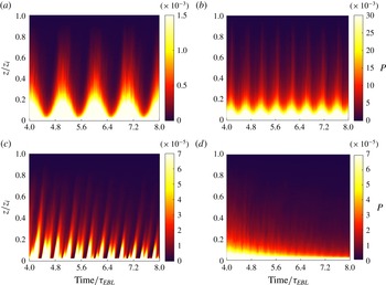
Space–time graphs of the dimensionless shear production (multiplied by
 $z_{i}/G^{3}$
) for cases (a) 3 SO, (b) 4 RO, (c) 5 FO and (d) 6-VFO.

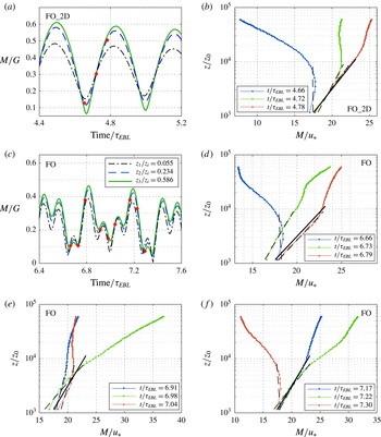
To further examine the turbulence dynamics in the cases of figure 5, spacetime graphs of the shear-production terms are plotted in figure 6. The production oscillations are correlated with the mean velocity fluctuations, and the magnitude of this term decreases in height (except perhaps some parts of the FO case which will be discussed in § 4.4). Another important feature to observe in these graphs is the phase lag of the sinusoidal behaviour of the TKE budget at different heights. One could notice approximately 10–30 min phase lag, for example, between the time series extrema at
 $z/z_{i}=0.055$
and 0.234 in figure 5 (the higher elevations lag the lower ones), which is related to the faster response of the smaller eddies near the surface compared with the larger eddies further aloft, as well as to the time required for the shear-produced turbulence at the surface to be transported to higher levels. For instance, a lag of approximately 30 min between the two shown heights can be observed in the production and dissipation terms of figure 5(d) at
 $t=3.2\unicode[STIX]{x1D70F}_{EBL}$
and the minima of figure 5(b) at
 $t=3.6\unicode[STIX]{x1D70F}_{EBL}$
. These lags are more apparent in figure 6, where they are illustrated by the vertical tilt of the patterns of strong production, which are particularly clear in the FO case (figure 6
c). We will quantitatively calculate this lag between two heights in § 6.
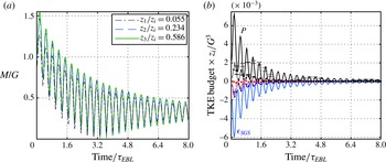
The role of the variability in the forcing direction, at a constant magnitude, is also explored. This is shown in figure 7, which depicts the velocity (figure 7 a) and TKE budget (figure 7 b) time series of the 2D fast oscillation. As in the 1D FO case, various TKE terms are directly responding to the mean velocity oscillations, and the mean decreases with time due to the filtering of the forcing by the damped-oscillator dynamics. Therefore, time variabilities in the magnitude or the direction of the forcing seem to result in comparable responses and mean–turbulence interactions.
The
 $M$
(a) and TKE budget (b) time series for case 7 FO_2D. The TKE budget terms are as defined in the legend of figure 5(h). The error bars on the production term are the residuals of the budget, reflecting the uncertainty in the budget terms.

4.3 The role of the Coriolis force
The final case investigated (figure 8) illustrates the influence of the Coriolis force on the dynamics of the EBL. This simulation has the same variable forcing as the RO case, but the mean flow responds very differently and no resonance is observed. This distinct behaviour is due to the fact that the 12.5 h forcing in RO matches the mean EBL time scale (
 $\unicode[STIX]{x1D70F}_{EBL}=2\unicode[STIX]{x03C0}/f_{c}\approx 12.5$
h), while it does not represent any special frequency for the UNR case where the Coriolis effect is not present. Hence, such a forcing time scale in the RO case leads to the resonance phenomena and to an increase in the magnitude of the velocity and TKE budgets, whereas in the UNR case the velocity decreases exponentially. This exponential decay can be exactly predicted by the solutions of the two coupled ODEs which form a reduced model of the Reynolds-averaged Navier–Stokes (RANS) equations, as derived in Momen & Bou-Zeid (Reference Momen and Bou-Zeid2016) by setting
 $f_{c}=0$
(which results in a mass–damper system with no spring). Despite the significant differences in the mean response, the TKE budget terms peak and fall with a small lag relative to
 $M$
as in the EBL simulations, suggesting that turbulence is only influenced by the mean variability it experiences, regardless of the driving forcing variability that modulates the mean. This is consistent with the observation that in the MKE equation (2.6), the forcing variability appears through
 $\overline{u_{i}}\unicode[STIX]{x2202}\overline{p}/\unicode[STIX]{x2202}x_{i}$
, while in the TKE equation (2.7) the forcing variability does not appear directly. Thus, the forcing pressure gradient interacts with the mean, which then interacts with turbulence. However, turbulence is not directly modulated by the variability in the pressure forcing. Therefore, these cases indicate that in general the turbulence and the mean interactions are similar in flows with and without rotation (as long as
 $Ro$
is not too small, since rotation can damp turbulence at small
 $Ro$
), but the dynamics of the mean is strongly affected by the Coriolis force. In other words, the Coriolis force only directly influences the mean dynamics (2.4), while it does not explicitly appear in the TKE budget equation (2.5) and has only an indirect influence on the TKE. Hence, the main difference between the UNR case (analogous to a mass–damper system) and other cases in this paper (analogous to mass–spring–damper systems) is in their mean response to the imposed forcing, while their TKE budget dynamics are expected to be similar according to (2.5), which is confirmed by our LES results.
Furthermore, the simulations of this case are in agreement with the LES results of other papers, which have investigated oscillatory flows driven by harmonic pressure gradients without rotation. For instance, the production and dissipation terms in figure 8(b) show one complete sinusoidal cycle at each imposed pressure-gradient sinusoidal oscillation (without the appearance of other oscillatory time scales such as the
 $\unicode[STIX]{x1D70F}_{EBL}$
). This is similar to the results of Salon et al. (Reference Salon, Armenio and Crise2007), although in our simulation the TKE budgets, as well as
 $M$
, are decreasing from the initial conditions to reach the statistically steady-state oscillations (where the crests of
 $M$
do not vary between cycles).
The
 $M$
(a) and TKE budget (b) time series for case 8 UNR. The solid lines in (b) show the budgets for
 $z/z_{i}=0.234$
and the lines with dots are for
 $z/z_{i}=0.055$
. The error bars on the production term are the residuals of the budget, reflecting the uncertainty in the budget terms.

4.4 Turbulence quasi-equilibrium and normalized TKE budget
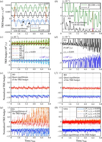
We define the ‘quasi-equilibrium with the mean’ as the conditions where the turbulence statistics of a flow at any point in time are equivalent to those that would be generated if the current mean values at that same point in time were steady. This definition can be directly assessed from the present simulation results. For instance, figure 9(a) displays the mean velocity and the production and dissipation time series for both steady-state and slow-oscillation cases. As figure 9(a) indicates, when the mean velocities of both simulations are the same, the production and dissipation terms have the same values (the oscillating and straight horizontal lines intersect), implying that the turbulence is in quasi-equilibrium with the mean. In such conditions, if the turbulence statistics are normalized properly with the mean, they will collapse independent of the imposed variations. Examples of this non-dimensionalization with the mean velocity for three cases are shown in figure 9(c). We will use this normalization to develop a turbulence closure model based on the mean variables in § 6. Nevertheless, in the FO case, the production term departs from its steady-state equivalent values (figure 9 b), and hence the turbulence is out of equilibrium with the mean, and normalization with the mean yields a highly variable times series (figure 9 d).
Given that turbulence varies with the unsteady mean, and some mean-normalized quantities like TI vary in time, we will also normalize the TKE budget terms by a turbulence statistic of order 2 (TKE production) to further examine the departure of turbulence from quasi-equilibrium. Production–dissipation balance is often used to assert turbulence equilibrium (Pope Reference Pope2000); we will also examine the transport terms here.
When the forcing time period is larger than the turbulence time scale
 $\unicode[STIX]{x1D70F}_{f}\gg \unicode[STIX]{x1D70F}_{t}$
, if quasi-equilibrium holds, it is expected that the production-normalized TKE budget terms would only be functions of height, independent of the forcing function that is imposed on them. The SO and RO cases shown in figure 9(e,f) indeed seem to be close to a quasi-equilibrium, since the variations of the time series of the TKE budget terms are moderate (dissipation/production ratio varies by less than 20 % of its mean signal). This implies that although the TI of these cases varies in time, as shown in figure 4, the TKE budget dynamics equilibrates fast and maintains quasi-steady budget profiles. In other words, the relative shapes of the budget profiles in these cases remain the same, while their magnitude might change in time; the profiles will collapse if properly normalized (e.g. by shear production as we did here, or by the mean velocity as in figure 9
c). This is expected, since the turbulence time scale is smaller than the imposed forcing time period, such that turbulence should have enough time to adapt itself to the exerted slow variations.
The ‘quasi-equilibrium of the turbulence with the mean’ is examined for case 3 SO (a) and case 5 FO (b). Normalized TKE budget by the mean for cases where the turbulence is in quasi-equilibrium with the mean flow (c) and for case FO lacking quasi-equilibrium (d, the maximum rises up to 0.3). Relative TKE budget time series for cases 3 SO (e), 4 RO (f), 5 FO (g) and 6 VFO (h).

More surprisingly perhaps, when the forcing time period is much smaller than the time scale of the turbulence,
 $\unicode[STIX]{x1D70F}_{f}\ll \unicode[STIX]{x1D70F}_{t}$
, we still observe the same quasi-equilibrium behaviour. As figure 9(h) shows, the VFO case also exhibits the same dynamics in which the normalized TKE budget profile preserves its shape and does not change much in time. This behaviour is due to the fact that the imposed variable forcing is very fast, such that the turbulence cannot respond accordingly; its effect is thus to integrate or filter the very fast variations of the mean signal over its time scale
 $\unicode[STIX]{x1D70F}_{t}$
, as discussed above. Only the slow decay of the mean of this case modifies the TKE budget, and turbulence adapts to this gradual change. As we discussed before, the turbulence contains a spectrum of eddies with time scales
 ${\leqslant}\unicode[STIX]{x1D70F}_{t}$
. Therefore, there exist some smaller turbulent eddies that interact with this very fast oscillatory variation in the mean flow. That is the reason for the relatively higher variation of the normalized TKE budget of the VFO case in figure 9(h) compared with the SO and RO cases in figure 9(e,f), resulting in a weaker quasi-equilibrium state with the mean for the VFO in comparison with other slower cases shown in figure 9(c). Despite this fact, larger more energetic eddies cannot respond to this very fast oscillation, and this results in a filtered TKE production that remains near a quasi-equilibrium state. In other words, the most energetic eddies of the turbulence cannot respond to the very fast oscillations of the imposed forcing and the mean at time scales smaller than
 $\unicode[STIX]{x1D70F}_{t}$
, and hence it filters out the imposed fast fluctuations of the mean flow and only responds to the filtered signal, which is a slow decay here.
Nevertheless, if the forcing and turbulence time scales are comparable,
 $\unicode[STIX]{x1D70F}_{f}\approx \unicode[STIX]{x1D70F}_{t}$
, the TKE budget will no longer be in quasi-equilibrium. For instance, figure 9(g) shows that in the FO case, the forcing strongly alters the TKE budget profiles. Such behaviour is more pronounced when the mean velocity decreases, and consequently the shear production is reduced significantly, while other TKE terms do not decrease as fast as production. In the FO simulation, the production term becomes nearly zero even at the surface during some periods, as illustrated in figure 6(c). However, there is always a minimum level of shear production in the VFO (figure 6
d) and other cases (figure 6
a,b). Similar behaviour could also be observed when such oscillation occurs in both directions (as shown for the case FO_2D in appendix B, figure 17). It should be noted that in the FO case, the magnitude of the forcing changes, while in the FO_2D case, only the direction of the forcing varies. Yet, in both cases, the TKE budget profile changes and a quasi-equilibrium turbulence state is no longer observed. Moreover, this out of equilibrium phenomenon, and the subsequent failure of similarity laws like the log-law shown in the next section, will not only occur at this specific forcing frequency. It will occur over a range of forcing frequencies that have comparable time periods to the turbulence time scale; for example, when
 $\unicode[STIX]{x1D70F}_{f}=6.25$
h, an analogous EBL response will emerge (see appendix B for an illustration).
5 Log-law validity under unsteady pressure gradients
The logarithmic velocity profile might not hold when turbulence is not in quasi-equilibrium, since the unsteady turbulent stresses could interact with the mean dynamics in complex uncharacteristic ways. However, as noted in the introduction, mean unsteadiness and even departure from equilibrium does not necessarily preclude the formulation of self-similarity laws (Tennekes & Lumley Reference Tennekes and Lumley1972), and the log-law could therefore still apply under some conditions. This is particularly plausible here, since, despite the fact that the TI displayed some strong disequilibrium signals for all simulations, the normalized TKE budget terms indicated that the production, dissipation and transport of TKE were in fact in equilibrium for many of the cases we study. To investigate this question, the velocity profiles are examined in different phases and in seven cases (SF, SO, RO, FO, VFO, FO_2D and UNR). For the steady forcing case, the velocity profiles in the inertial layer will follow the logarithmic similarity law with a von Kármán constant
 $\unicode[STIX]{x1D705}$
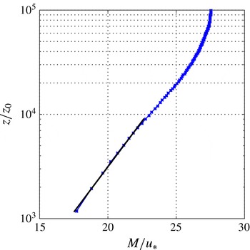
of approximately 0.4 (see Pope Reference Pope2000, chap. 7), as expected if the LES model is adequate. This is indeed reproduced by our LES, as shown in the semi-log plot of figure 10, where the time averaging is only over 10 min for consistency with the unsteady cases, the blue line displays the LES profile and the solid black line is the fitted log-law with
 $\unicode[STIX]{x1D705}=0.4$
. This black line with the same
 $\unicode[STIX]{x1D705}$
(and intercept) is used as a basis for comparison for the unsteady cases to assess departures from the steady-state log-law profile.
Log-law wind profile for case 1 (steady forcing).

In order to make such an assessment, we define the following dimensionless parameters that quantify the departure from a log-law in the first 90 m (
 $0.09z_{i}$
, or first 12 grid nodes) above the surface:
 $$\begin{eqnarray}\displaystyle \left.\begin{array}{@{}c@{}}\displaystyle \unicode[STIX]{x1D6FE}\equiv \frac{\sqrt{\text{var}(M^{+}-M_{log\,fit}^{+})}}{\overline{M^{+}}},\\ \displaystyle \unicode[STIX]{x1D6FE}_{d}\equiv \frac{\unicode[STIX]{x1D6FE}}{\unicode[STIX]{x1D6FE}_{0}},\quad \displaystyle \unicode[STIX]{x1D705}_{d}\equiv \frac{\unicode[STIX]{x1D705}_{FittedLog}}{\unicode[STIX]{x1D705}_{0}},\end{array}\right\} & & \displaystyle\end{eqnarray}$$
where
 $M^{+}=M/u_{\ast }$
(
 $u_{\ast }$
, the friction velocity, is computed at the same time as the profile of
 $M$
is taken; both are averaged over a horizontal plane and over short periods in table 1). The term
 $\unicode[STIX]{x1D6FE}_{d}$
is a normalized curvature parameter (akin to a normalized coefficient of determination for the fit) that indicates the departure from a log profile compared with the steady-state simulation for which
 $\unicode[STIX]{x1D6FE}_{0}=0.3$
. The term
 $\unicode[STIX]{x1D705}_{d}$
is a slope parameter normalized by the value
 $\unicode[STIX]{x1D705}_{0}=0.4$
that holds for the steady simulation reference. It measures the departure of the slope of the fit from the conventional steady-state value.

5.1 Weak to moderate departures from the log-law
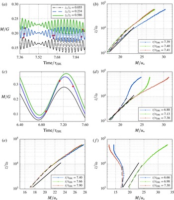
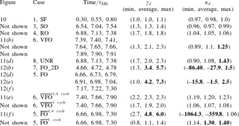
The velocity profiles for the unsteady cases that display a moderate departure from the steady-state log-law are first examined at three distinct times in a single cycle, selected close to the end of the simulation: first at the trough of the cycle, then at a quarter period, and finally at a half-period corresponding to the peak. For cases with a moderate departure from the log-law, we plot the three distinct instantaneous profiles for the various cases in figure 11(a–d). The plots show that the normalized wind profile is not constant and varies according to the phase of the imposed unsteady forcing, indicating some moderate departures from the log-law similarity in cases VFO and UNR. The steady-state log-law is denoted by the solid black lines, while the dashed lines show the log-curves fitted to each instantaneous profile and are used to compute the parameters in (5.1); these parameters are provided in table 2 for all of the unsteady simulations. We will consider here that the log-law is not applicable in cases with more than 25 % change in the slope parameter or a tripling in the curvature parameter. These are ad hoc thresholds, but we will use them for a convenient distinction of moderate versus strong departure from the log-law profile.
For RO and SO simulations, the instantaneous (
 $\unicode[STIX]{x1D6FE}_{d}$
,
 $\unicode[STIX]{x1D705}_{d}$
) values varied in the ranges (1.0–2.0, 0.9–1.1) at different times (figures not shown, see table 2), implying that, based on our criteria, the log-law is ‘applicable’ in these cases in the sense that it can be a useful prognostic tool despite some inaccuracy. The VFO case, on the other hand, shows moderate departures from the log-law, as shown in figure 11(b). Table 2 shows that the curvature parameter in this case is approximately 2–3 times larger than the steady-state case, and the von Kármán constant increases or decreases based on the phase. The
 $\unicode[STIX]{x1D705}_{d}$
value is higher by approximately 25 % when
 $t=7.41\unicode[STIX]{x1D70F}_{EBL}$
and lower by 11 % when
 $t=7.64\unicode[STIX]{x1D70F}_{EBL}$
in the VFO (relative to a value of 1 which would mean that the slope is the same as the steady-state case). However, the trend of increasing wind speed with height persists, despite significant departure from the log-law at some instants. The unsteady pressure forcing with no Coriolis case also shows comparably moderate departures from the log-law profiles. Figure 11(d) and table 2 indicate a 10 % decrease and up to 43 % increase in the slope parameter, with approximately a doubling of the curvature parameter.
Wind profiles for strong departures from the log-law: case 7 FO_2D (a,b) and case 5 FO (c–f).

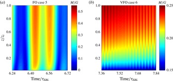
Space–time graphs of wind-profile evolutions for (a) case 5 FO and (b) case 6 VFO.

Log-law departures in seven cases; the cases with an overbar over the name are for averaged profiles. The strong departures from the log-law, for which it is not applicable based on our criteria, are shown in bold.

5.2 Strong departures from the log-law
The fast-oscillation simulations show strong log-law departures. For instance, the FO_2D case exhibits clear log-law failure, as shown in figure 12(b). The
 $\unicode[STIX]{x1D705}_{d}$
values in table 2 for this case are very far from unity, reaching
 $-86.4$
at
 $t=4.66\unicode[STIX]{x1D70F}_{EBL}$
(inverted velocity profile), with a sixfold increase in the curvature parameter. Furthermore, very significant departures are observed in the FO case. Figure 12(c–f) assesses the log-law validity in this case, here for multiple cycles and multiple times in each cycle. The wind profile is drastically different, and the log-law fails to describe it at most times. Figure 13 exhibits the space–time graph for part of the FO simulation (figure 13
a) compared with the VFO case (figure 13
b). Inverted velocity profiles can be observed at
 $t\approx 6.32\unicode[STIX]{x1D70F}_{EBL}$
and
 $t\approx 6.68\unicode[STIX]{x1D70F}_{EBL}$
in figure 13(a), while velocity profiles are not inverted in figure 13(b). Moreover, during some periods (e.g.
 $t\approx 6.28\unicode[STIX]{x1D70F}_{EBL}$
and
 $6.64\unicode[STIX]{x1D70F}_{EBL}$
in figure 13
a) the magnitude of the velocity is nearly zero throughout the EBL in the FO case. Table 2 shows that the curvature parameter increases significantly in this case. It becomes approximately seven times larger at
 $t=6.98\unicode[STIX]{x1D70F}_{EBL}$
and
 $t=7.30\unicode[STIX]{x1D70F}_{EBL}$
. The slope parameter is also modified substantially: at
 $t=6.66\unicode[STIX]{x1D70F}_{EBL}$
and
 $t=7.30\unicode[STIX]{x1D70F}_{EBL}$
, it even becomes negative, indicating that the wind velocity is decreasing with height (inverted velocity profiles). This phenomenon usually occurs when
 $M$
is close to a local minimum and the pressure-gradient force changes the wind direction.
5.3 Log-law validity for the averaged profiles
We also examined the cycle-averaged wind profiles to see whether the log-law is valid if the velocities are averaged in time. Figure 11(e) presents the VFO case averaged over a quarter of its forcing cycle (5 min), and figure 11(f) shows the profiles averaged over a quarter forcing cycle of the FO case (approximately 47 min). The last four rows of table 2 provide the curvature and slope parameters of these profiles averaged over a quarter and a full forcing cycle. The full-cycle-averaged values display less eccentricity from the steady-state reference than the instantaneous profiles, but they still exhibit large departures for the FO case, and consequently the log-law is still not applicable for the FO case (in practical applications, the forcing will not be cyclic and hence time averaging to recover a log-law is even less feasible). The full-cycle-averaged profiles of the VFO case match the log-law reasonably well.
To summarize, these strong departures in the instantaneous and averaged wind profiles indicate that the classic log-law fails to accurately describe the wind profile in these fast-oscillating unsteady cases. In particular, when the imposed forcing time scale is of the order of the turbulence time scale, where the interactions between the mean and turbulence are strongly out of equilibrium, these departures are significant. On the other hand, for the slow and resonant forcing, as well as for the very fast forcing, the log-law could offer a reasonable model of the wind profile (see supplementary material available at https://doi.org/10.1017/jfm.2017.76 for further information about wind velocity animations and the corresponding evolution of the TKE production and dissipation profiles under unsteady forcing).
6 Implications of the unsteady forcing on turbulence closures
One of the major challenges in unsteady flows is that many turbulence closure models rely on the equilibrium assumption. Therefore, the quality of numerical simulation techniques relying on the Reynolds-averaged approach would be adversely affected in such flows (one could assume that the small parameterized scales in LES have a much shorter eddy turnover time and thus equilibrate much faster with the mean and larger eddies, although in some cases this also becomes a questionable assumption). In this section, we investigate the impact of the lack of equilibrium on some basic turbulence closure models.
For cases that are close to equilibrium, and based on the observation that the unsteady behaviour of the turbulence follows from the variability of the mean flow, we will attempt to model turbulent parameters such as the shear production using only mean parameters, as done in turbulence closure schemes. To that end, we first model the shear-production term using a turbulent-viscosity closure as
 $$\begin{eqnarray}\displaystyle P=-\overline{u^{\prime }w^{\prime }}\frac{\unicode[STIX]{x2202}\overline{u}}{\unicode[STIX]{x2202}z}-\overline{v^{\prime }w^{\prime }}\frac{\unicode[STIX]{x2202}\overline{v}}{\unicode[STIX]{x2202}z}\approx \unicode[STIX]{x1D708}_{T}\left(\frac{\unicode[STIX]{x2202}\overline{M}}{\unicode[STIX]{x2202}z}\right)^{2}. & & \displaystyle\end{eqnarray}$$
Then, we invoke Prandtl’s mixing-length concept in formulating the eddy viscosity, a concept known to fail under disequilibrium conditions (Tennekes & Lumley Reference Tennekes and Lumley1972, chap. 2), and assume the following classic characteristic length and velocity scales to express it:
 $$\begin{eqnarray}\displaystyle v^{\ast }\equiv \sqrt{\overline{e}},\quad L^{\ast }\equiv C_{1}v^{\ast }\frac{1}{\unicode[STIX]{x2202}\overline{M}/\unicode[STIX]{x2202}z}=C_{1}\frac{\sqrt{\overline{e}}}{\unicode[STIX]{x2202}\overline{M}/\unicode[STIX]{x2202}z}\Rightarrow \unicode[STIX]{x1D708}_{T}=C_{2}v^{\ast }L^{\ast }=C_{1}C_{2}\frac{\overline{e}}{\unicode[STIX]{x2202}\overline{M}/\unicode[STIX]{x2202}z}. & & \displaystyle\end{eqnarray}$$
Now, one can combine (6.1) and (6.2) and assume that
 $\overline{e}\sim \overline{E}$
(the validity of this assumption for the various cases can be checked in figure 4 since
 $\overline{e}/\overline{E}=2TI^{2}$
) to model the shear production as a function of mean variables as
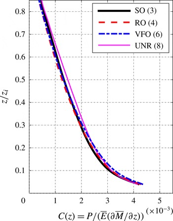
 $$\begin{eqnarray}\displaystyle P(t+\unicode[STIX]{x1D70F}_{0},z)=C(z)\overline{E}(t,z)\frac{\unicode[STIX]{x2202}\overline{M}}{\unicode[STIX]{x2202}z}(t,z)\Rightarrow C=\frac{P}{\displaystyle \overline{E}\frac{\unicode[STIX]{x2202}\overline{M}}{\unicode[STIX]{x2202}z}}. & & \displaystyle\end{eqnarray}$$
It should be noticed that in (6.3) we also introduced a time lag,
 $\unicode[STIX]{x1D70F}_{0}$
, between the mean and turbulence parts to allow for the stresses and strain to equilibrate and produce TKE (the MKE and gradients in the equation are thus evaluated at
 $t$
). It can be determined as the lag that maximizes the discrete cross-correlation of
 $P$
and
 $\overline{E}\unicode[STIX]{x2202}\overline{M}/\unicode[STIX]{x2202}z$
, and it was found to be approximately 10–30 min at different heights (for example, at
 $z/z_{i}=0.055$
the lag was
 ${\approx}10$
min, while it was found to be
 ${\approx}20$
–30 min at
 $z/z_{i}=0.234$
; lags less than the temporal averaging periods, listed in table 1, could not be determined).
Equation (6.3) expresses the shear production as a function of the MKE and mean shear stress. This formulation is similar to the classic 1.5-order closure, with the difference that our eddy viscosity is a function of MKE rather than TKE (so an additional transport equation for the TKE is not needed in this case).
This model in (6.3) strongly relies on equilibrium assumptions; if it is accurate,
 $C$
should be constant in time and only a function of height. Its failure would then imply turbulence that is out of equilibrium with its mean flow. Figure 14 depicts the time series of
 $C$
for four unsteady cases; this function is found to be time-independent and only height-dependent in cases SO, RO and VFO. There are some small oscillations that are negligible compared with the mean value (5 %–25 % fluctuations around the mean). However, case 5 (FO) displays a distinctive behaviour again, and oscillations grow as the interactions between the turbulence and the mean flow become more intractable when the imposed forcing frequency is of the order of the turbulence natural frequency. Equation (6.3) fails to model production based on the mean variables only in case FO (and FO_2D, which is not shown), and further research is required to understand and model the associated complex dynamics. Nevertheless, in the other investigated cases, (6.3) yields promising results according to figure 14 and
 $C$
is only a function of height, independent of the forcing frequency. This implies that equilibrium-based closures, even based on MKE, would in general work for these cases.
Turbulent production variation with respect to the suggested mean model for (a) case 3 (SO), (b) 4 (RO), (c) 5 (FO) and (d) 6 (VFO).

The
 $C$
function profiles for four unsteady cases averaged over the whole simulation time.

The time and forcing independence of
 $C$
can also be deduced from its profiles. Figure 15 shows
 $C(z)$
profiles for four unsteady simulations, including the three cases of figure 14. The UNR simulation exhibits a similar
 $C(z)$
function to other cases since the TKE budget dynamics is not directly influenced by the Coriolis force, as indicated in § 4.3. This figure confirms that
 $C(z)$
seems universal for any imposed variable pressure gradient, except when
 $\unicode[STIX]{x1D70F}_{f}\sim \unicode[STIX]{x1D70F}_{t}$
. It should be noted that once
 $C(z)$
is found (e.g. from figure 15), all other unsteady TKE budget terms (like transport and dissipation) could be represented in terms of this model by multiplying the resulting production in (6.3) by the production-normalized budgets of figure 9.
To sum up, this section again illustrates that over a range of forcing time scales (where
 $\unicode[STIX]{x1D70F}_{f}\approx \unicode[STIX]{x1D70F}_{t}$
), mean and turbulence interaction is not in quasi-equilibrium. Closure models like the one we tested here, as well as the majority of other low-order closures and similarity theories like the log-law, will not be valid since they are based on equilibrium concepts. Higher-order closures or other non-equilibrium-based approaches would then be needed. However, when
 $\unicode[STIX]{x1D70F}_{f}$
is not of the same order as
 $\unicode[STIX]{x1D70F}_{t}$
, the moderate disequilibrium that can arise does not preclude the use of some equilibrium-based models.
7 Conclusion
Mean–turbulence interactions under variable forcing are investigated via LES. Eight cases are simulated to show the unsteady behaviour of the Ekman boundary layer. The first two cases are steady cases and examine the impact of the LES SGS modelling on the TKE budget. It is shown that TKE budget terms, in particular the transport and dissipation, are sensitive to the selected SGS model; nevertheless, all investigated models fail to exactly close the budget. Subsequently, turbulence intensity statistics from unsteady simulations are shown to vary with time; periodic slow changes in the slow-forcing case, for example, result in similar periodic behaviour for the turbulence statistics. The analyses allow us to answer the three questions posed in the introduction as follows.
Question (1): the response of the mean flow only depends on
 $\unicode[STIX]{x1D70F}_{f}/\unicode[STIX]{x1D70F}_{EBL}$
; when
 $\unicode[STIX]{x1D70F}_{f}>\unicode[STIX]{x1D70F}_{EBL}$
, the mean adjusts to the forcing and only exhibits variability at a time scale
 $\unicode[STIX]{x1D70F}_{f}$
, while when
 $\unicode[STIX]{x1D70F}_{f}<\unicode[STIX]{x1D70F}_{EBL}$
, the mean could vary at both time scales. The turbulence only interacts directly with the mean flow and its variability time scale, not with the forcing pressure gradient. However, since
 $\unicode[STIX]{x1D70F}_{t}/\unicode[STIX]{x1D70F}_{EBL}$
is always
 $\ll 1$
, the turbulence response depends primarily on
 $\unicode[STIX]{x1D70F}_{t}/\unicode[STIX]{x1D70F}_{f}$
since the mean can exhibit variability at
 $\unicode[STIX]{x1D70F}_{f}$
that is then passed on to the turbulence fields. When
 $\unicode[STIX]{x1D70F}_{f}\gg \unicode[STIX]{x1D70F}_{t}$
, turbulence adjusts to the relatively slow variations in the mean; when
 $\unicode[STIX]{x1D70F}_{f}\sim \unicode[STIX]{x1D70F}_{t}$
, turbulence is strongly out of equilibrium; while when
 $\unicode[STIX]{x1D70F}_{f}\ll \unicode[STIX]{x1D70F}_{t}$
, turbulence filters some of the fast variability of the mean flow and is again closer to a quasi-equilibrium state. It should be noted that
 $\unicode[STIX]{x1D70F}_{t}$
is mainly estimated here as the turnover time of the largest eddies, i.e. the longest time scale of the turbulence spectrum that would be first approached by
 $\unicode[STIX]{x1D70F}_{f}$
as it decreases. In addition, these general findings in terms of the dimensionless time-scale ratios apply regardless of their actual dimensional value.
Question (2): the production-normalized TKE budget terms indicate that when the forcing is slow (
 $\unicode[STIX]{x1D70F}_{f}\gg \unicode[STIX]{x1D70F}_{t}$
), turbulence is in a quasi-equilibrium condition and the shape of the normalized TKE budget profile does not change. The same behaviour occurs for the very fast forcing (
 $\unicode[STIX]{x1D70F}_{f}\ll \unicode[STIX]{x1D70F}_{t}$
), in which the turbulence filters out the very fast oscillations of the mean into a smoothed signal (MKE–TKE conversion). Only when the forcing time scale is of the order of the turbulence time scale (
 $\unicode[STIX]{x1D70F}_{f}\sim \unicode[STIX]{x1D70F}_{t}$
) do we observe this quasi-equilibrium breaking down.
Question (3): the log-law in unsteady boundary layers was examined in § 5 quantitatively by introducing two non-dimensional metrics (slope and curvature parameters). The results illustrate that the instantaneous wind profiles in the unsteady pressure forcing cases with
 $\unicode[STIX]{x1D70F}_{f}\gg \unicode[STIX]{x1D70F}_{t}$
or
 $\unicode[STIX]{x1D70F}_{f}\ll \unicode[STIX]{x1D70F}_{t}$
depart from the log-law at various times in the cycle, although their averaged profiles show a better match to the steady logarithmic wind profile (the log-law is not always accurate even in these cases). On the other hand, 1D and 2D fast-forcing scenarios in which the forcing time scale is comparable with the turbulence time scale showed unusual wind profiles and very strong departures from the log-law, both instantaneously and in the averaged results. These departures increased when the velocity magnitude was close to a local minimum and when the flow direction was changing.
Finally, the implications of the unsteady forcing on the turbulence closures were investigated using a model for the turbulence production, which is based on the mixing-length concept and mean variables. This model was shown to work well, and the coefficient of the model, which relates the production to mean variables, remains independent of time and forcing in the unsteady cases SO, RO, VFO, and UNR (the time-averaged profiles of all of these cases collapsed well). However, it did not give satisfactory results for the FO case, where highly complex and atypical interactions between the turbulence and mean dynamics arise, and this case requires further study. In the FO simulation (
 $\unicode[STIX]{x1D70F}_{f}\approx \unicode[STIX]{x1D70F}_{t}$
), where turbulence is highly out of equilibrium, uncommon inverted velocity profiles are observed (indicating strong log-law departures), and 1- and 1.5-order equilibrium-based closures cannot capture the dynamics or reproduce the LES results. Second- and higher-order or non-equilibrium closures might yield better results in unsteady Reynolds-averaged Navier–Stokes simulations.
All analyses therefore confirm that the strongest departures from equilibrium occurs when
 $\unicode[STIX]{x1D70F}_{f}\sim \unicode[STIX]{x1D70F}_{t}$
, and hence better performance of equilibrium-based models or laws is observed when there is a disparity between the two time scales, i.e. when
 $\unicode[STIX]{x1D70F}_{f}\gg \unicode[STIX]{x1D70F}_{t}$
and even when
 $\unicode[STIX]{x1D70F}_{f}\ll \unicode[STIX]{x1D70F}_{t}$
.
Acknowledgements
The authors acknowledge support from the Cooperative Institute for Climate Science (CICS) of Princeton University and the National Oceanographic and Atmospheric Administration (NOAA) under grant no. 344-6127, and the Physical and Dynamic Meteorology Program of the National Science Foundation under AGS-1026636. The simulations were performed on the computing clusters of the National Center for Atmospheric Research under project no. P36861020.
Supplementary material
Supplementary material is available at https://doi.org/10.1017/jfm.2017.76.
Appendix A. Verifying the small effect of the SGS TKE term
$(\unicode[STIX]{x1D70E}_{kk})$
on the TKE budget

The SGS TKE term is modelled as
 $$\begin{eqnarray}\displaystyle \unicode[STIX]{x1D70E}_{kk}=\frac{\langle \unicode[STIX]{x1D613}_{ii}\rangle }{2\left[\left(\displaystyle \frac{\overline{\unicode[STIX]{x1D6E5}}}{\widetilde{\unicode[STIX]{x1D6E5}}}\right)^{2/3}-1\right]}, & & \displaystyle\end{eqnarray}$$
where
 $\unicode[STIX]{x1D613}_{ii}=\overline{\widetilde{u_{i}}\widetilde{u_{i}}}-\overline{\widetilde{u_{i}}}\,\overline{\widetilde{u_{i}}}$
is the trace of the Leonard stress tensor, and
 $\overline{\unicode[STIX]{x1D6E5}}=2\unicode[STIX]{x1D6E5}$
and
 $\widetilde{\unicode[STIX]{x1D6E5}}=4\unicode[STIX]{x1D6E5}$
are the widths of the test and grid filters respectively (see Knaepen, Debliquy & Carati Reference Knaepen, Debliquy and Carati2002; Salesky & Chamecki Reference Salesky and Chamecki2012). Figure 16 displays the SF case results in which we have also included the
 $\unicode[STIX]{x1D70E}_{kk}$
in our computations. It is clear from this figure that inclusion of this term will slightly improve the TKE budget closure at
 $0.07<z/z_{i}<0.15$
, but it worsens the closure close to the wall (
 $z/z_{i}<0.07$
). Hence, there is no significant advantage in including this term and we do not obtain a very different picture in the TKE budget terms. It only changes the pressure correlation term as expected from (2.3), and adds the SGS TKE transport term.
The TKE budget terms for the SF case, including the SGS TKE term. The
 $e_{SGS}$
term in this figure denotes the transport of the SGS TKE by the turbulent eddy term,
 $-(1/3)(\unicode[STIX]{x2202}\overline{w^{\prime }\unicode[STIX]{x1D70E}_{kk}^{\prime }}/\unicode[STIX]{x2202}z)$
.

Velocity magnitude (a), TKE (b), TKE budget (c) and normalized TKE budget time series (d) for case FO_2D.

Velocity magnitude (a), TKE (b), TKE budget (c) and production-normalized TKE budget time series (d) for case IO.

Appendix B. Other cases with out of equilibrium TKE budget
Two cases with highly variable relative TKE budget terms (in addition to FO) are shown in this appendix. In both forcing scenarios, the turbulence is not in quasi-equilibrium. As figure 17(d) exhibits, the turbulence is not in equilibrium anymore when the direction of imposed pressure gradient rotates with a period close to the turbulence time scale.
B.1 Case FO_2D
This case is shown in figure 17.
B.2 Case IO (intermediate oscillation)
All of the numerical details of this case are similar to the FO case, except the imposed forcing time scale which is 6.25 h here, and therefore
 $$\begin{eqnarray}\displaystyle U_{g}=\cos (2\unicode[STIX]{x03C0}t/6.25),\quad V_{g}=0. & & \displaystyle\end{eqnarray}$$
Many abrupt jumps in the relative budget time series are observed in figure 18, demonstrating a lack of equilibrium of turbulence.