1 Introduction
Precise estimation of the diffusion constant of biomolecules is important for quantitative analysis of transport in living cells. It is also crucial for the proper interpretation of biophysical experiments, such as fluorescence correlation spectroscopy, ultracentrifugation or dynamic light scattering. If the internal structure of the macromolecule is rigid, then its transport properties can be efficiently calculated by a variety of methods, including bead modelling (Bloomfield, Dalton & Van Holde Reference Bloomfield, Dalton and Van Holde1967; de la Torre & Bloomfield Reference de la Torre and Bloomfield1978; Byron Reference Byron2008; Zuk, Cichocki & Szymczak Reference Zuk, Cichocki and Szymczak2018), boundary element methods (Allison Reference Allison1999; Aragon Reference Aragon2004) or path integral techniques (Kang, Mansfield & Douglas Reference Kang, Mansfield and Douglas2004; Mansfield & Douglas Reference Mansfield and Douglas2008; Juba et al. Reference Juba, Audus, Mascagni, Douglas and Keyrouz2017).
However, it becomes increasingly clear that the structure of most biomolecules is flexible and fluctuating rather than rigid. Even well-folded proteins undergo slow, large-scale movements of subunits, which are referred to as protein breathing (Makowski et al. Reference Makowski, Rodi, Mandava, Minh, Gore and Fischetti2008). In many cases, one finds flexible linkers or loops connecting domains, allowing for inter-domain hinge motions or flap motions (Jacobs, Kuhn & Thorpe Reference Jacobs, Kuhn and Thorpe2002; Thorpe et al. Reference Thorpe, Chubynsky, Hespenheide, Menor, Jacobs, Kuhn, Zavodszky, Lei, Rader and Whiteley2005). For example, HIV-1 protease has two molecular flaps which move a distance of up to 7 Å when the enzyme becomes associated with a substrate (Ishima et al. Reference Ishima, Freedberg, Wang, Louis and Torchia1999). At the extreme end of the flexibility spectrum are proteins with disordered sequences that fail to form a permanent tertiary structure but can adopt a variety of transient conformations. These are referred to as intrinsically disordered proteins (IDPs) (Dyson & Wright Reference Dyson and Wright2005; Oldfield & Dunker Reference Oldfield and Dunker2014). It is estimated that 30 %–50 % of eukaryotic proteins contain at least one long disordered region. These proteins participate in important regulatory functions in the cell, including transcription, translation and cell signalling (Galea et al. Reference Galea, Wang, Sivakolundu and Kriwacki2008; Oldfield et al. Reference Oldfield, Meng, Yang, Yang, Uversky and Dunker2008; Dosztányi, Mészáros & Simon Reference Dosztányi, Mészáros and Simon2009). Several IDPs have been shown to be associated with various diseases such as cancer and neurodegenerative diseases (Iakoucheva et al. Reference Iakoucheva, Brown, Lawson, Obradović and Dunker2002; Uversky, Oldfield & Dunker Reference Uversky, Oldfield and Dunker2008). The importance of IDPs in cellular processes calls for rethinking of the classical structure–function paradigm (Wright & Dyson Reference Wright and Dyson1999; Berlow, Dyson & Wright Reference Berlow, Dyson and Wright2018), that protein function depends on a fixed three-dimensional structure.
Flexibility of the molecules brings considerable complications into the calculation of their hydrodynamic properties. Instead of the 6 degrees of freedom of a rigid molecule, we now need to deal with
 $6N$
degrees of freedom, with
 $N$
standing for the number of rigid subunits. To make the problem tractable, a number of approximations have been adopted over the years. Perhaps the simplest was introduced by Kirkwood & Riseman (Reference Kirkwood and Riseman1948) in the context of polymer solutions. Here, the polymer is assumed to be rigidly frozen in one of a large number of possible conformations. Transport properties are then calculated by treating the molecule as a rigid body, and the results are averaged over the equilibrium ensemble. Such a rigid body approximation was later taken up by Zimm (Reference Zimm1980, Reference Zimm1982) and de la Torre and co-workers (Schmidt, Cifre & de la Torre Reference Schmidt, Cifre and de la Torre2012; de la Torre Reference de la Torre2016), and incorporated into the HYDRO set of programs (de la Torre Reference de la Torre2016); however, the validity of this approximation and its accuracy remain unclear (Schmidt et al.
Reference Schmidt, Cifre and de la Torre2012).
To facilitate the analytical treatment of polymer dynamics, Kirkwood & Riseman (Reference Kirkwood and Riseman1948) introduced an additional ‘pre-averaging’ approximation in which the chain conformation-dependent hydrodynamic disturbance, induced by the motion of the polymer, is replaced by its equilibrium average over all chain conformations. However, while pre-averaged Kirkwood–Riseman theory was successful in explaining many dynamical properties of polymers, a number of studies (Zimm Reference Zimm1980; de La Torre, Jimenez & Freire Reference de La Torre, Jimenez and Freire1982) indicated that the errors introduced by this approach can be considerable.
An important observation, due to Fixman (Reference Fixman1981, Reference Fixman1983), is that the diffusion coefficient in a flexible macromolecule will also be time-dependent, with well-defined short- and long-time limits. The difference between the two is due to memory effects related to the relaxation of the internal coordinates of the molecule. Due to the positiveness of the memory function, the long-time diffusion coefficient can be shown to be always smaller than the short-time diffusivity (Fixman Reference Fixman1983). These effects have been further studied by Liu & Dünweg (Reference Liu and Dünweg2003) using the Zwanzig–Mori projection operator technique.
From another angle, Wegener (Reference Wegener1982) and Harvey, Mellado & García de la Torre (Reference Harvey, Mellado and García de la Torre1983) have considered relatively simple molecules with one flexible joint, which was taken into account by the introduction of appropriate generalized coordinates. One problem that they encountered was that the diffusion coefficient turned out to be dependent on the choice of the origin. In an insightful paper, Wegener (Reference Wegener1985) proposed that the appropriate reference point (which he called centre of diffusion,
 $C_{D}$
) should correspond to the minimal short-time diffusion coefficient, but he was not able to find an explicit formula for its position. He also hypothesized that the minimal short-time diffusion coefficient is equal to the long-time diffusion coefficient, accessible by experimental measurements.
Below, we show how to find the centre of diffusion for a rather broad class of elastic macromolecules, which can be represented as a collection of
 $N$
beads interacting with a general intramolecular potential. We also demonstrate that the short-time diffusion coefficient calculated at the centre of diffusion is not equal to the long-time diffusion coefficient (as claimed by Wegener), but the difference between the two is small and can be calculated at a modest computational expense.
Snapshots of the trajectory of an elastic molecule undergoing Brownian motion.

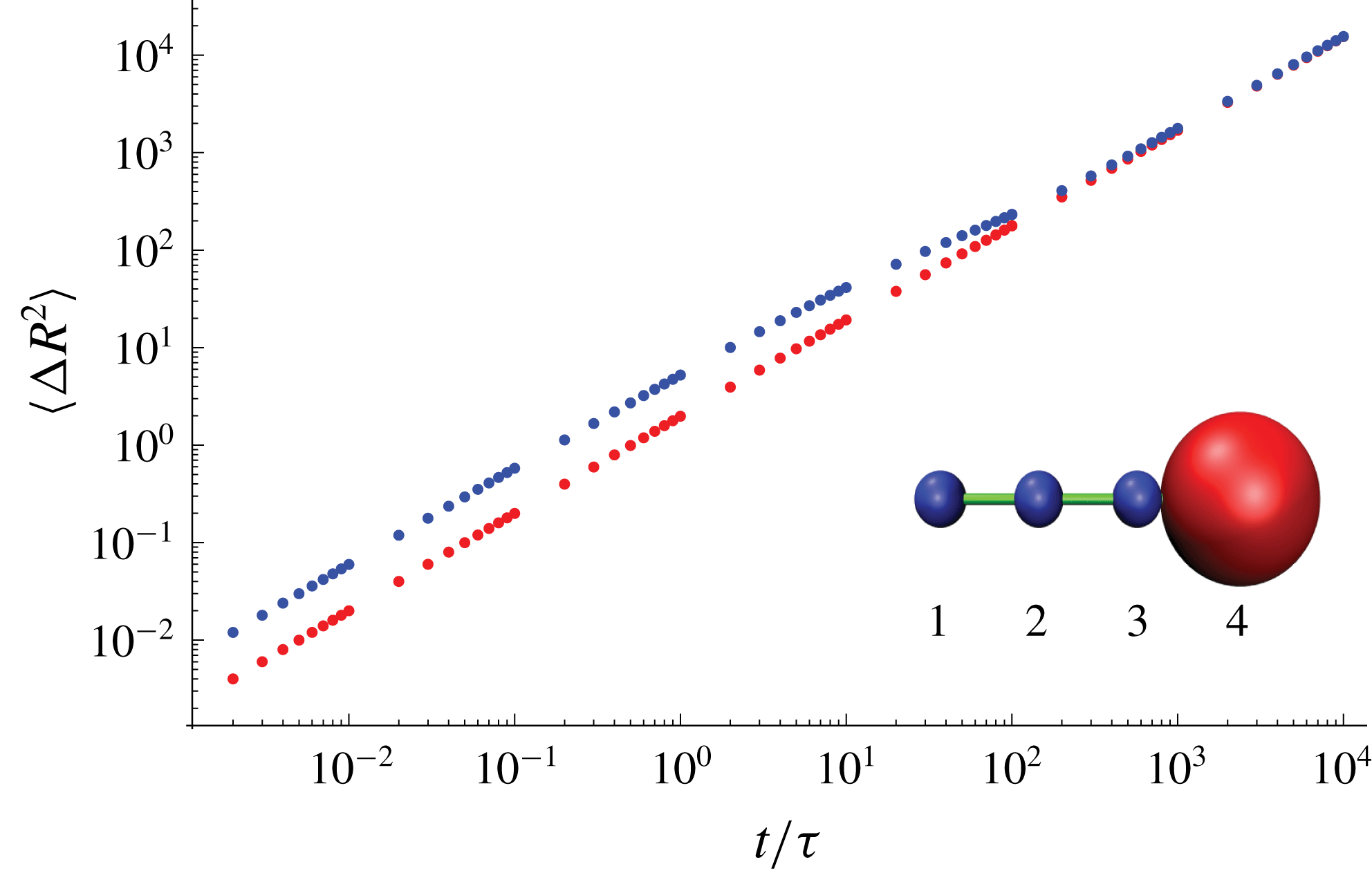
Before we turn to a formal description of the method, let us first briefly present the main problems one encounters when analysing the diffusion of flexible molecules, using a simple example. Consider a small linear molecule, which consists of four beads – three of radius
 $a$
, and the fourth of radius
 $3a$
(figure 1). The beads are connected with harmonic springs of an equilibrium length
 $l_{0}=4a$
and spring constant
 $k=5.5kT/a$
. The hydrodynamic interactions between them are described within the Rotne–Prager approximation (Rotne & Prager Reference Rotne and Prager1969; Yamakawa Reference Yamakawa1970; Zuk et al.
Reference Zuk, Wajnryb, Mizerski and Szymczak2014). The evolution is calculated using the Brownian dynamics (BD) algorithm (Ermak & McCammon Reference Ermak and McCammon1978). In figure 2, we show the mean square displacement of the centres of the first and fourth bead. The distances are measured in
 $a$
, whereas the time unit is
 $\unicode[STIX]{x1D70F}=a^{2}/6D_{0}$
, where
 $D_{0}$
is the diffusion coefficient of a single bead of radius
 $a$
.
Mean square displacement (MSD) of a given point on a molecule versus time. The molecule consists of four beads connected with springs, as shown in the inset. The blue points correspond to the MSD of bead no. 1, whereas the red points correspond to that of bead no. 4.

There are several observations to be made based on the data in figure 2. First, for a given point
 $P$
of the molecule, the mean square displacement
 $\unicode[STIX]{x0394}R^{2}(t)$
is linear in time only at very short and very long times. The corresponding definitions of the short-time and long-time translational diffusion coefficient read:
 $$\begin{eqnarray}\langle (\boldsymbol{R}(t)-\boldsymbol{R}(0))^{2}\rangle \sim 6D_{s}(P)t,\quad t\rightarrow 0\end{eqnarray}$$
and
 $$\begin{eqnarray}\langle (\boldsymbol{R}(t)-\boldsymbol{R}(0))^{2}\rangle \sim 6D_{l}\,t,\quad t\rightarrow \infty .\end{eqnarray}$$
In the above,
 $\langle \cdots \rangle$
denotes the equilibrium average.
Second, the value of the short-time diffusion coefficient depends on the choice of the point that we track. Conversely, the long-time diffusivity is independent of the choice of the reference point. Finally, the value of the long-time diffusion coefficient is always smaller than that of its short-time counterpart. For the data in figure 2,
 $D_{l}=0.2898\pm 0.0002$
(in the units of
 $D_{0}$
), whereas the short-time diffusion coefficients are
 $D_{s}(1)=1$
(for the small bead) and
 $D_{s}(4)=1/3$
(for the large bead).
In experiments, the long-time diffusion coefficient is usually measured, due to the time scales involved in either fluorescence correlation spectroscopy, ultracentrifugation or dynamic light scattering. However, a direct assessment of
 $D_{l}$
in the BD simulations is very hard, if not impossible, for complex biomolecules. The main reason for this is a relatively slow convergence of the value of
 $D_{l}$
with the time interval over which the data is collected, due to the presence of relatively long relaxation times, related to the relaxation of the internal degrees of freedom as well as the rotation of the macromolecule as a whole. The acquirement of statistically meaningful BD data on these time scales is computationally expensive, mostly due to the necessity of generating a normally distributed random vector with a covariance determined by the
 $N$
-particle diffusion tensor. To give an example, the generation of figure 2 requires three days of computation time on a Intel Xeon E5-2670 workstation at 2.50 GHz. The bead models of real biological macromolecules are much more complex, comprising hundreds of beads. Since the computational complexity of simulating the BD trajectory increases with the number of beads (
 $N$
) as
 $N^{3}$
, the calculation becomes prohibitively expensive to carry out.
2 Short- and long-time diffusion coefficient
Turning to a formal description, let us introduce a general model of a macromolecule as a collection of beads of different sizes (possibly overlapping), suspended in a viscous fluid and interacting with potential forces. We assume that the Reynolds number is small and thus the motion is an overdamped one. On a mesoscopic level (Van Kampen Reference Van Kampen1992), the state of such a system is then described by positions of the centres of the beads
 $\boldsymbol{X}=(\boldsymbol{R}_{1},\boldsymbol{R}_{2},\ldots ,\boldsymbol{R}_{N})$
. An important step in the analysis is splitting
 $\boldsymbol{X}$
into the internal and external coordinates. The internal coordinates describe simply the relative positions of the beads with respect to each other
 $$\begin{eqnarray}\boldsymbol{X}_{int}=(\boldsymbol{R}_{12},\boldsymbol{R}_{23},\ldots ,\boldsymbol{R}_{N-1,N}),\end{eqnarray}$$
with
 $\boldsymbol{R}_{ij}=\boldsymbol{R}_{i}-\boldsymbol{R}_{j}$
. The external coordinate, on the other hand, describes the position of one specific point
 $P$
of the macromolecule in the laboratory frame. This position will be given by a vector
 $\boldsymbol{R}$
, which is a linear combination of the positions of the beads
 $$\begin{eqnarray}\boldsymbol{R}=x_{1}\boldsymbol{R}_{1}+x_{2}\boldsymbol{R}_{2}+\cdots +x_{N}\boldsymbol{R}_{N},\end{eqnarray}$$
with the non-negative coefficients
 $x_{i}$
summing up to one (that is,
 $\sum _{i=1}^{N}x_{i}=1$
). The configuration vector can thus be written as
 $\boldsymbol{X}=(\boldsymbol{R},\boldsymbol{X}_{int})$
. The vector of the coefficients
 $x_{i}$
will be denoted as
 $\boldsymbol{x}$
:
 $$\begin{eqnarray}\boldsymbol{x}=\{x_{1},x_{2},\ldots ,x_{N}\}.\end{eqnarray}$$
Note that for identical beads, the choice
 $x_{1}=x_{2}=\cdots x_{N}=1/N$
corresponds to the position of the centre of mass of the system.
The potential energy of particle interactions
 $U(\boldsymbol{X}_{int})$
is only a function of the internal coordinates,
 $\boldsymbol{X}_{int}$
. Similarly, the
 $N$
-particle mobility matrix
 $\unicode[STIX]{x1D741}$
describing the hydrodynamic interactions between the beads is also a function of
 $\boldsymbol{X}_{int}$
only. The mobility matrix links the velocities of the particles with the forces acting on them, according to
 $$\begin{eqnarray}\boldsymbol{U}_{i}=\mathop{\sum }_{j}\unicode[STIX]{x1D741}_{ij}\boldsymbol{F}_{j},\end{eqnarray}$$
where
 $\boldsymbol{U}_{i}$
is the velocity of bead
 $i$
and
 $\boldsymbol{F}_{j}$
is the force with which particle
 $j$
act on the fluid. Note that the mobility matrix needs to be positive-definite for all particle configurations (Happel & Brenner Reference Happel and Brenner1973).
Let
 $P(\boldsymbol{X},t)$
be the probability density of finding the system in configuration
 $\boldsymbol{X}$
at time
 $t$
, with the normalization
 $\int \text{d}\boldsymbol{X}\;P(\boldsymbol{X},t)=1$
, where
 $\text{d}\boldsymbol{X}=\text{d}\boldsymbol{R}\,\text{d}\boldsymbol{X}_{int}$
and
 $\text{d}\boldsymbol{X}_{int}=$
 $\text{d}\boldsymbol{R}_{12}\ldots \text{d}\boldsymbol{R}_{1N}$
. At equilibrium, the distribution becomes uniform in
 $\boldsymbol{R}$
and Boltzmannian in the internal coordinates – that is,
 $P^{eq}(\boldsymbol{X})=(1/V)P^{eq}(\boldsymbol{X}_{int})$
with
 $P^{eq}(\boldsymbol{X}_{int})\sim \text{e}^{-\unicode[STIX]{x1D6FD}U(\boldsymbol{X}_{int})}$
. The evolution of a Brownian system is governed by the generalized Smoluchowski equation
 $$\begin{eqnarray}\unicode[STIX]{x2202}_{t}P(\boldsymbol{X},t)={\mathcal{L}}(\boldsymbol{X})P(\boldsymbol{X},t),\end{eqnarray}$$
where
 $$\begin{eqnarray}{\mathcal{L}}(\boldsymbol{X})=\mathop{\sum }_{i,j=1}^{N}\frac{\unicode[STIX]{x2202}}{\unicode[STIX]{x2202}\boldsymbol{R}_{i}}\boldsymbol{\cdot }\unicode[STIX]{x1D63F}_{ij}(\boldsymbol{X}_{int})\boldsymbol{\cdot }\left(\frac{\unicode[STIX]{x2202}}{\unicode[STIX]{x2202}\boldsymbol{R}_{j}}+\unicode[STIX]{x1D6FD}\frac{\unicode[STIX]{x2202}U(\boldsymbol{X}_{int})}{\unicode[STIX]{x2202}\boldsymbol{R}_{j}}\right)\end{eqnarray}$$
is the evolution operator and
 $$\begin{eqnarray}\unicode[STIX]{x1D63F}_{ij}(\boldsymbol{X}_{int})=k_{B}T\unicode[STIX]{x1D741}_{ij}(\boldsymbol{X}_{int})\end{eqnarray}$$
is the diffusion matrix. Note that
 $\unicode[STIX]{x2202}/\unicode[STIX]{x2202}\boldsymbol{R}_{i}=x_{i}(\unicode[STIX]{x2202}/\unicode[STIX]{x2202}\boldsymbol{R})+\unicode[STIX]{x2202}/\unicode[STIX]{x2202}\boldsymbol{R}_{i,int}$
, where the second term on the right-hand side denotes the derivative with respect to
 $\boldsymbol{R}_{i}$
through the dependence on
 $\boldsymbol{X}_{int}$
.
In the following, we will characterize the motion of the point
 $\boldsymbol{R}$
(2.2) by introducing the time- and origin-dependent diffusion coefficient
 $$\begin{eqnarray}D(t,\boldsymbol{x})=\frac{1}{6}\frac{\text{d}}{\text{d}t}\langle [\boldsymbol{R}(t)-\boldsymbol{R}(0)]^{2}\rangle ,\end{eqnarray}$$
where
 $\langle \cdots \rangle$
denotes an equilibrium average (that is,
 $\langle A\rangle =\int A(\boldsymbol{X})P_{eq}(\boldsymbol{X})\,\text{d}\boldsymbol{X}$
) and
 $\boldsymbol{x}$
is the weight vector defined in (2.3). Note that here we adopt the convention that
 $P_{eq}(\boldsymbol{X})$
is always placed at the right-hand side of the integrand, which is important if
 $A$
is a differential operator.
Making use of the stationarity of the stochastic process governing the motion of the molecule,
 $$\begin{eqnarray}D(t,\boldsymbol{x})=-\frac{1}{3}\frac{\text{d}}{\text{d}t}\langle \boldsymbol{R}(t)\boldsymbol{\cdot }\boldsymbol{R}(0)\rangle =-\frac{1}{3}\frac{\text{d}}{\text{d}t}\text{Tr}\langle \boldsymbol{R}\boldsymbol{e}^{{\mathcal{L}}(\boldsymbol{X})\boldsymbol{t}}\boldsymbol{R}\rangle ,\end{eqnarray}$$
which allows us to express
 $D(t)$
in the following form (Akcasu Reference Akcasu1982; Fixman Reference Fixman1983; Cichocki & Hinsen Reference Cichocki and Hinsen1992; Liu & Dünweg Reference Liu and Dünweg2003):
 $$\begin{eqnarray}D(t,\boldsymbol{x})=D_{s}(\boldsymbol{x})-\int _{0}^{t}M(\unicode[STIX]{x1D70F},\boldsymbol{x})\,\text{d}\unicode[STIX]{x1D70F},\end{eqnarray}$$
where
 $$\begin{eqnarray}D_{s}(\boldsymbol{x})\equiv D_{s}(\boldsymbol{x})=-\frac{1}{3}\text{Tr}\langle \boldsymbol{R}{\mathcal{L}}(\boldsymbol{X})\boldsymbol{R}\rangle =\frac{k_{B}T}{3}\mathop{\sum }_{i,j=1}^{N}x_{i}x_{j}\langle \text{Tr}\,\unicode[STIX]{x1D741}_{ij}\rangle\end{eqnarray}$$
is the short-time diffusion coefficient and the memory function
 $M(t)$
is given by
 $$\begin{eqnarray}M(t,\boldsymbol{x})={\textstyle \frac{1}{3}}\text{Tr}\langle \boldsymbol{V}\text{e}^{{\mathcal{L}}_{int}(\boldsymbol{X}_{int})t}\boldsymbol{V}\rangle .\end{eqnarray}$$
Here,
 ${\mathcal{L}}_{int}(\boldsymbol{X}_{int})$
is the Smoluchowski operator
 ${\mathcal{L}}(\boldsymbol{X})$
, in which the derivatives with respect to
 $\boldsymbol{R}_{i}$
were replaced by the derivatives with respect to
 $\boldsymbol{R}_{i,int}$
. The particle flux,
 $\boldsymbol{V}$
, is given by
 $$\begin{eqnarray}\boldsymbol{V}={\mathcal{D}}(\boldsymbol{X})\boldsymbol{R}=\mathop{\sum }_{i,j=1}^{N}x_{j}\left\{\left[\frac{\unicode[STIX]{x2202}}{\unicode[STIX]{x2202}\boldsymbol{R}_{i,int}}\boldsymbol{\cdot }\unicode[STIX]{x1D63F}_{ij}(\boldsymbol{X}_{int})\right]-\unicode[STIX]{x1D6FD}\frac{\unicode[STIX]{x2202}U(\boldsymbol{X}_{int})}{\unicode[STIX]{x2202}\boldsymbol{R}_{i,int}}\boldsymbol{\cdot }\unicode[STIX]{x1D63F}_{ij}(\boldsymbol{X}_{int})\right\},\end{eqnarray}$$
where we have introduced the operator
 ${\mathcal{D}}(\boldsymbol{X})$
adjoint to
 ${\mathcal{L}}(\boldsymbol{X})$
, given by
 ${\mathcal{L}}(\boldsymbol{X})P^{eq}(\boldsymbol{X})\cdots \,$
 $=P^{eq}(\boldsymbol{X}){\mathcal{D}}(\boldsymbol{X})$
.
In biophysical experiments, a long-time diffusion coefficient is usually measured,
 $D_{l}=D(t=+\infty )$
, related to displacements much larger than the size of the molecule. Note that, for a bound system, the long-time diffusion coefficient does not depend on the choice of the tracked point
 $\boldsymbol{R}$
. Indeed, the difference of diffusion coefficients for two different choices of
 $\boldsymbol{x}$
follows
 $$\begin{eqnarray}D(t,\boldsymbol{x})-D(t,\boldsymbol{x}^{\prime })=-\frac{1}{3}\frac{\text{d}}{\text{d}t}\langle [\boldsymbol{R}(t)-\boldsymbol{R}^{\prime }(t)]\boldsymbol{\cdot }[\boldsymbol{R}(0)+\boldsymbol{R}^{\prime }(0)]\rangle ,\end{eqnarray}$$
where we have used (2.8) together with the condition of detailed balance. For a bound system, the vector
 $\boldsymbol{R}(t)-\boldsymbol{R}^{\prime }(t)$
is of a limited length; hence,
 $D(t,\boldsymbol{x})-D(t,\boldsymbol{x}^{\prime })\rightarrow 0$
as
 $t\rightarrow \infty$
. In our case this statement means that
 $D_{l}$
becomes independent of the choice of the coefficients
 $\boldsymbol{x}$
. On the other hand, both
 $D_{s}$
and
 $M(\unicode[STIX]{x1D70F})$
do depend on the choice of the reference point. We then obtain
 $$\begin{eqnarray}D_{l}=D_{s}(\boldsymbol{x})-\int _{0}^{+\infty }M(\unicode[STIX]{x1D70F};\boldsymbol{x})\,\text{d}\unicode[STIX]{x1D70F}.\end{eqnarray}$$
The direct computation of the long-time diffusion coefficient by means of BD simulation is computationally expensive (Liu & Dünweg Reference Liu and Dünweg2003; Schmidt et al.
Reference Schmidt, Cifre and de la Torre2012). However, a relatively simple estimate of
 $D_{l}$
can be obtained by the analysis of (2.15). First, note that the right-hand side of the above relation is the difference between two non-negative quantities. This is a consequence of the fact that the Smoluchowski equation (2.5) governing the evolution of the system describes overdamped dynamics with detailed balance (Van Kampen Reference Van Kampen1992). Consequently, the lower the value of
 $D_{s}(\boldsymbol{x})$
, the closer it is to the long-time diffusion coefficient. The upper bound for
 $D_{l}$
can then be obtained by taking the minimum of the short-time diffusion coefficient
 $D_{s}(\boldsymbol{x})$
with respect to
 $\boldsymbol{x}$
.
The formal procedure is the following. We introduce a matrix
 $\unicode[STIX]{x1D63C}$
indexed by the particle labels (
 $i,j$
) as
 $$\begin{eqnarray}\unicode[STIX]{x1D608}_{ij}={\textstyle \frac{1}{3}}\text{Tr}\langle \unicode[STIX]{x1D741}_{ij}\rangle .\end{eqnarray}$$
We can then express
 $D_{s}(\boldsymbol{x})$
as
 $$\begin{eqnarray}D_{s}(\boldsymbol{x})=k_{B}T(\boldsymbol{x}^{\text{T}}\boldsymbol{\cdot }\unicode[STIX]{x1D63C}\boldsymbol{\cdot }\boldsymbol{x}),\end{eqnarray}$$
where the superscript T stands for the transposition. Next, we solve the variational problem of finding the minimum of
 $D_{s}(\boldsymbol{x})$
with respect to
 $\boldsymbol{x}$
. The normalization condition for
 $\boldsymbol{x}$
can be expressed as
 $\boldsymbol{x}^{\text{T}}\boldsymbol{\cdot }\boldsymbol{i}=1$
, where
 $\boldsymbol{i}$
is a column vector of ones. The variational problem for
 $D_{s}(\boldsymbol{x})$
with respect to
 $x_{i}$
,
 $i=1,2,\ldots ,N$
, is then
 $$\begin{eqnarray}\unicode[STIX]{x1D6FF}\{\boldsymbol{x}^{\text{T}}\boldsymbol{\cdot }\unicode[STIX]{x1D63C}\boldsymbol{\cdot }\boldsymbol{x}-\unicode[STIX]{x1D706}(\boldsymbol{x}^{\text{T}}\boldsymbol{\cdot }\boldsymbol{i}-1)\}=0.\end{eqnarray}$$
From the above, we get the extremum condition
 $2\unicode[STIX]{x1D63C}\boldsymbol{\cdot }\boldsymbol{x}_{min}-\unicode[STIX]{x1D706}\boldsymbol{i}=0$
. This corresponds to a minimum, due to the positive definiteness of the matrix
 $\unicode[STIX]{x1D63C}$
. Explicitly,
 $$\begin{eqnarray}\boldsymbol{x}_{min}=\frac{\unicode[STIX]{x1D706}}{2}\unicode[STIX]{x1D63C}^{-1}\boldsymbol{\cdot }\boldsymbol{i},\end{eqnarray}$$
where the coefficient
 $\unicode[STIX]{x1D706}$
can be obtained from the normalization condition, yielding
 $\unicode[STIX]{x1D706}/2=(\boldsymbol{i}^{\text{T}}\boldsymbol{\cdot }\unicode[STIX]{x1D63C}^{-1}\boldsymbol{\cdot }\boldsymbol{i})^{-1}$
, so that
 $$\begin{eqnarray}\boldsymbol{x}_{min}=\frac{\unicode[STIX]{x1D63C}^{-1}\boldsymbol{\cdot }\boldsymbol{i}}{\boldsymbol{i}^{\text{T}}\boldsymbol{\cdot }\unicode[STIX]{x1D63C}^{-1}\boldsymbol{\cdot }\boldsymbol{i}}=\frac{\displaystyle \mathop{\sum }_{j}(\unicode[STIX]{x1D63C}^{-1})_{ij}}{\displaystyle \mathop{\sum }_{i,j}(\unicode[STIX]{x1D63C}^{-1})_{ij}}.\end{eqnarray}$$
Finally, we get the minimum value of the short-time diffusion coefficient as
 $$\begin{eqnarray}D_{s}(\boldsymbol{x}_{min})=k_{B}T\boldsymbol{x}_{min}^{\text{T}}\boldsymbol{\cdot }\unicode[STIX]{x1D63C}\boldsymbol{\cdot }\boldsymbol{x}_{min}=k_{B}T\frac{1}{\boldsymbol{i}^{\text{T}}\boldsymbol{\cdot }\unicode[STIX]{x1D63C}^{-1}\boldsymbol{\cdot }\boldsymbol{i}}=k_{B}T\frac{1}{\displaystyle \mathop{\sum }_{i,j}(\unicode[STIX]{x1D63C}^{-1})_{ij}}.\end{eqnarray}$$
3 Discussion
Returning to the example of the chain molecule of figure 2, for the Rotne–Prager model of hydrodynamic interactions, (2.21) gives the diffusion constant of
 $D_{s}(\boldsymbol{x}_{min})=0.2919$
, which is less than 0.7 % off the long-time diffusion coefficient obtained in the BD simulations. On the other hand, the Kirkwood formula, which corresponds to calculating the diffusion coefficient in the geometrical centre of a macromolecule (that is, for
 $x_{i}=1/N$
), gives
 $$\begin{eqnarray}D_{K}=\frac{k_{B}T}{N^{2}}\mathop{\sum }_{i,j}(\unicode[STIX]{x1D63C})_{ij}=0.375,\end{eqnarray}$$
which significantly overestimates the value of the long-time diffusion coefficient. In fact,
 $D_{K}$
is even larger than the single-body diffusion coefficient of the largest bead (that is, for
 $x_{i}=\unicode[STIX]{x1D6FF}_{4i}$
), which is
 $D_{4}=k_{B}TA_{44}=0.33(3)$
. A slightly better estimate can be obtained by taking the centre of mass of the macromolecule, with
 $x_{i}\sim a_{i}^{3}$
, where
 $a_{i}$
is the radius of the
 $i$
th bead. In this case
 $D_{CM}=0.312$
, which is still, however, about 8 % off the value obtained from the BD. Another possibility is to take the weight proportional to the friction coefficients of individual beads (that is,
 $x_{i}\sim a_{i}$
). This leads to
 $D=0.309$
, about 7 % off the BD value.
Note that (2.21) itself is exact, as no approximations have been made in the derivation. One can use it for different models of hydrodynamic interactions – both in simple models (for example, Oseen or Rotne–Prager far-field approximation (Kim & Karrila Reference Kim and Karrila1991)) or in more sophisticated approaches, like the multipole expansion method (Mazur & van Saarloos Reference Mazur and van Saarloos1982; Felderhof Reference Felderhof1988; Cichocki et al.
Reference Cichocki, Felderhof, Hinsen, Wajnryb and Bławzdziewicz1994). The interaction potential can also be arbitrary, provided that it keeps the system bound. Importantly, the estimation of the long-time diffusion coefficient using (2.21) is not intensive computationally, since it does not require BD simulations. All that is needed are the equilibrium averages
 $\unicode[STIX]{x1D608}_{ij}$
(2.16), which can be obtained, for example, by Monte Carlo sampling (Binder Reference Binder1995).
In polymer physics, pre-averaging approximation is popular (Kirkwood & Riseman Reference Kirkwood and Riseman1948; Zimm Reference Zimm1956; Dubois-Violette & De Gennes Reference Dubois-Violette and De Gennes1967; Yamakawa Reference Yamakawa1971; Bird et al.
Reference Bird, Hassager, Armstrong and Curtiss1987; Doi & Edwards Reference Doi and Edwards1988; Prakash Reference Prakash1999), in which the diffusion matrix
 $\unicode[STIX]{x1D63F}_{ij}$
is replaced in the evolution equation by its equilibrium average. This leads to a significant simplification of the dynamics. The particle flux (2.13) is then simply
 $$\begin{eqnarray}\boldsymbol{V}(\boldsymbol{x})=-\unicode[STIX]{x1D6FD}\mathop{\sum }_{i,j=1}^{N}\boldsymbol{F}_{i}\unicode[STIX]{x1D608}_{ij}x_{j},\end{eqnarray}$$
where we have used the fact that
 $\langle \unicode[STIX]{x1D63F}_{ij}\rangle =\unicode[STIX]{x1D608}_{ij}\boldsymbol{I}$
. In particular, if
 $\boldsymbol{x}$
corresponds to the diffusion centre, then the flux vanishes, since
 $\boldsymbol{V}(\boldsymbol{x}_{min})\sim \sum \boldsymbol{F}_{i}=0$
. Hence, within the pre-averaging approximation, the memory function at the centre of diffusion vanishes; consequently, the long-time diffusion coefficient at this point is equal to its short-time counterpart. In fact, as shown in Zimm (Reference Zimm1956), Yamakawa (Reference Yamakawa1971), Bird et al. (Reference Bird, Hassager, Armstrong and Curtiss1987), Öttinger (Reference Öttinger1987, Reference Öttinger1996) with the pre-averaged dynamics, the motion of the centre of resistance separates out from that of the internal configuration and becomes a Markov process. In this literature,
 $\boldsymbol{x}_{min}$
is usually called ‘centre of resistance’, since it also has the property that the net torque of hydrodynamic forces around this point vanishes during a uniform translation of the molecule relative to the fluid (Zimm Reference Zimm1956; Yamakawa Reference Yamakawa1971). However, these properties of
 $\boldsymbol{x}_{min}$
hold only within the pre-averaging approximation (Bird et al.
Reference Bird, Hassager, Armstrong and Curtiss1987; Öttinger Reference Öttinger1987). To avoid confusion regarding the properties of
 $\boldsymbol{x}_{min}$
, we have decided to call it ‘centre of diffusion’, following Wegener (Reference Wegener1985), who coined that term for a point inside the molecule where the diffusion coefficient is minimal.
If we go beyond the pre-averaging approximation, the memory function no longer vanishes, and we expect a small difference between the long-time diffusion coefficient and its short-time counterpart, calculated at
 $\boldsymbol{x}_{min}$
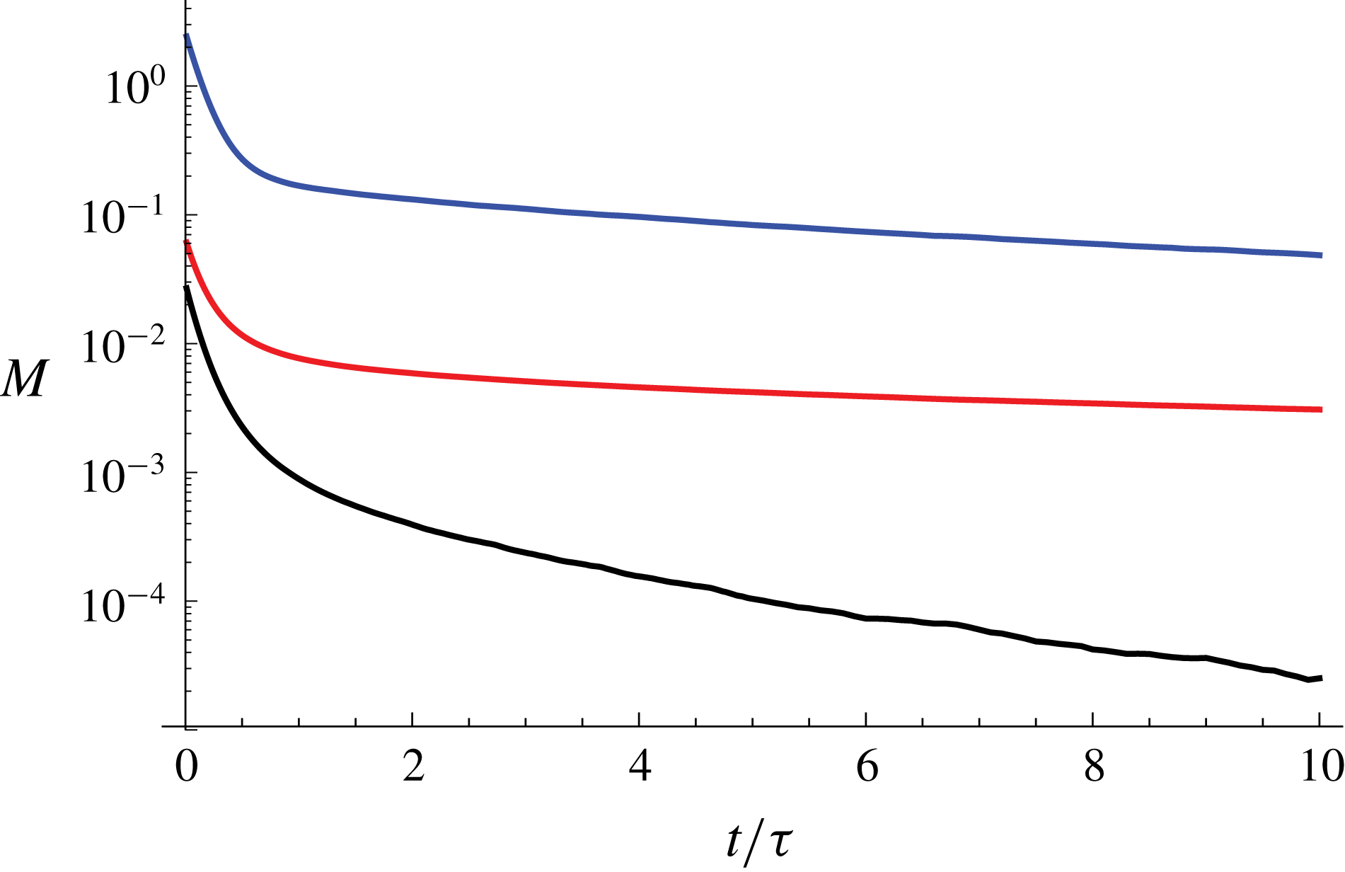
. This can be estimated by a direct calculation of the memory function given by (2.12). For our chain molecule, the memory function is shown in figure 3. We present there
 $M(t)$
for three different points of the molecule – one of the small beads (no. 1 in the inset of figure 2), the large bead (no. 4) and the centre of diffusion. The two former points exhibit exponential tails with the same characteristic decay time, connected with the rotation of the system as a whole. At the same time, the dynamics of the centre of diffusion shows a much smaller memory contribution. Even more importantly, the decay of
 $M(t)$
is now much faster – the long relaxation time connected with the slowest decaying mode is not present. This means that the calculation of memory correction to the diffusion coefficient at
 $\boldsymbol{x}_{min}$
does not require the generation of long Brownian trajectories. Already the integration up to
 $T=5$
gives
 $\int _{0}^{\text{T}}M(t)\,\text{d}t=0.002$
, which differs just by 5 % from the integral up to
 $T=100$
. Note that the memory correction itself is just 0.7 % of the long-time diffusivity, when calculated at the centre of diffusion. Contrastingly, the memory contribution to
 $D_{l}$
calculated at bead no. 1 corresponds to as much as 250 % of the final value, whereas that calculated at bead no. 4 is approximately 15 %.
The memory function
 $M(t)$
given by (2.12) for three different points on the molecule – bead no. 1 (blue), bead no. 4 (red) and the centre of diffusion (black).

Finally, let us briefly recall the case of a rigid macromolecule. In such a case, the memory function can be calculated analytically (Cichocki, Ekiel-Jezewska & Wajnryb Reference Cichocki, Ekiel-Jezewska and Wajnryb2012; Cichocki, Ekiel-Jeżewska & Wajnryb Reference Cichocki, Ekiel-Jeżewska and Wajnryb2015) and it can be shown that there exists a reference point for which the memory function vanishes; thus the mean square displacement of this point is linear over the entire time range.
In summary, we have presented a simple and accurate method of estimating the experimentally relevant long-time diffusivity of elastic macromolecules, based on the minimization of the short-time diffusion coefficient with respect to the tracked point. The method becomes exact within the pre-averaging approximation. In the case considered here, the long-time diffusivity is overestimated slightly (within 1 %) using this method. The exact value of this difference can be estimated by calculating the memory function,
 $M(t)$
, at the centre of diffusion, where the short-time diffusivity is minimal. This calculation, although involving dynamical simulations, is relatively inexpensive, since
 $M(t)$
decays at this point on a much faster time scale than at any other point of the macromolecule. The computational simplicity of the method is crucial for the efficient estimation of diffusion coefficients of large and complex elastic macromolecules, the bead models of which involve hundreds of components.
Naturally, the accuracy of the method will depend on the system studied, including the number of beads, their sizes and interbead potentials. It seems, however, that elimination of the slowest decaying mode in the memory function at
 $\boldsymbol{x}_{min}$
will in general produce a high-accuracy estimate of
 $D_{l}$
. The full assessment of the accuracy of the method will only be possible if the relaxation times corresponding to the Smoluchowski dynamics (2.5) are estimated, which should be the subject of further investigations.
Acknowledgement
This work was partially supported by grant no. UMO-2016/22/E/NZ1/00656 from the National Science Center, Poland.