INTRODUCTION
Interest in biofuels, including bio-ethanol, has increased both in the USA and across the rest of the world. Wheat grain has been an important raw material (feedstock) for ethanol production, especially in Canada (Husky Energy 2009) and Europe (European Bioethanol Fuel Association 2009). In addition, there has been experimental scaled production of ethanol from cellulosic wheat straw, e.g. in Canada (Iogen Corporation 2009). In the USA, there is a mandate to use 136 billion (i.e. 109) litres of bio-ethanol by 2022, of which at least 79·3 billion litres must come from sources other than maize starch, such as cellulosic feedstocks (US Congress 2007). In 2009, bio-ethanol production in the USA was 47·4 billion litres, of which more than 0·90 was produced from maize grain (Renewable Fuels Association 2010). Wheat is a potential alternative feedstock that could be used to meet the increased demand for bio-ethanol in the USA. The production of cellulosic ethanol from wheat straw is especially promising for increasing the bio-ethanol production capacity.
One major reason for the interest in bio-ethanol, including wheat-ethanol, is its potential to reduce the emission of greenhouse gases (GHG) by its replacement of fossil fuels (von Blottnitz & Curran Reference von Blottnitz and Curran2007; Borjesson Reference Borjesson2009). It is claimed that the ongoing increase in the global air temperature is partly caused by GHG emissions (Intergovernmental Panel on Climate Change (IPCC) 2006). Winter wheat grain and straw have potential as a bio-ethanol feedstock in the south-eastern USA; in this region, winter wheat is normally grown between two summer crops, such as soybean or peanut; it is usually planted in November–December and harvested in May–June (Lee et al. Reference Lee, Buntin, Culpepper, Harris, Martinez and Smith2008). However, a large proportion of cropland in the south-eastern USA is left fallow during the winter period (United States Department of Agriculture: National Agricultural Statistics Service 2009). Consequently, there is cropland available within the south-eastern USA that could be used for the production of winter wheat for ethanol purposes. Future cropping scenarios in the south-eastern USA could also involve a shift from major summer crops, notably cotton, which is normally rotated with winter fallow, towards soybean–winter wheat or peanut–winter wheat rotations. Historically, crop production in the south-eastern USA has varied substantially among these and other crops (United States Department of Agriculture: National Agricultural Statistics Service 2004, 2009) due to shifting prices and demand for agricultural crops over time.
Grain and straw yields of winter wheat in the south-eastern USA vary considerably among years due to weather variability (United States Department of Agriculture: National Agricultural Statistics Service 2004, 2009). This yield variation may also be different due to spatial climate patterns (SERCC 2009) and soil variability (Soil Survey Staff 2009) within the south-eastern USA. The impact of weather variability on crop growth and yield is normally difficult to predict prior to and during the cropping season. Consequently, crop management inputs such as tillage practices and fertilizer applications are not well correlated to yield of wheat: a low yield due to unfavourable weather conditions often entails greater crop management inputs per unit harvested yield. For wheat-ethanol production, such unpredictable variability in local weather conditions impacts not only the amount of ethanol that can be produced but also the amounts of GHG that are emitted per unit of wheat-ethanol produced. The reason for this influence is that crop management practices are associated with GHG emissions. These emissions should be accounted for when determining the total effect on GHG emissions of replacing fossil fuels with wheat-ethanol. In fact, it has previously been shown that cropping-related emissions substantially affect the potential to reduce GHG emissions by replacing fossil fuel with wheat-ethanol (Borjesson Reference Borjesson2009) as well as ethanol from maize (Liska et al. Reference Liska, Yang, Bremer, Klopfenstein, Walters, Erickson and Cassman2009). GHG emissions in wheat cropping, for example, come from the combustion of fossil fuels in various cropping operations and the production of chemical fertilizers. Also, GHG emissions from the soil due to alterations in soil management practices significantly impact the total emissions (Franzluebbers et al. Reference Franzluebbers, Hons and Zuberer1998; De Klein et al. Reference De Klein, Novoa, Ogle, Smith, Rochette, Wirth, McConkey, Mosier, Rypdal, Eggleston, Buendia, Miwa, Ngara and Tanabe2006). Given crop management practices that are constant or largely unchanged by weather variability during the growing season, a low yield due to unfavourable weather conditions would result in larger amounts of GHG emissions per unit of ethanol produced than would a high yield.
Winter wheat growth and yield as a response to weather and soil conditions and crop management practices can be simulated with crop growth models (Weir et al. Reference Weir, Bragg, Porter and Rayner1984; Eckersten & Jansson Reference Eckersten and Jansson1991; Porter et al. Reference Porter, Jamieson and Wilson1993; Jamieson et al. Reference Jamieson, Semenov, Brooking and Francis1998; Gillett et al. Reference Gillett, Crout, Stokes, Sylvester-Bradley and Scott1999; Atkinson et al. Reference Atkinson, Kettlewell, Poulton and Hollins2008). For example, the Cropping System Model (CSM)-CERES-Wheat model (Ritchie et al. Reference Ritchie, Singh, Godwin, Bowen, Tsuji, Hoogenboom and Thornton1998) has been applied to determine wheat growth under various environmental conditions throughout the world (Bannayan et al. Reference Bannayan, Crout and Hoogenboom2003; Nain et al. Reference Nain, Dadhwal and Singh2004; Barbieri et al. Reference Barbieri, Rozas and Echeverria2008; Langensiepen et al. Reference Langensiepen, Hanus, Schoop and Grasle2008; Xiong et al. Reference Xiong, Conway, Holman and Lin2008). For the south-eastern USA, crop growth models have previously been applied to determine the impact of climate, weather and soil variability on crops other than wheat, e.g. maize (Garcia y Garcia et al. Reference Garcia y Garcia, Guerra and Hoogenboom2008), cotton (Garcia y Garcia et al. Reference Garcia y Garcia, Guerra and Hoogenboom2008; Zamora et al. Reference Zamora, Jose, Jones and Cropper2009) and peanut (Paz et al. Reference Paz, Fraisse, Hatch, Garcia y Garcia, Guerra, Uryasev, Bellow, Jones and Hoogenboom2007). For the same region, crop growth models have been used to assess the impact of climate and soil variability on energy balances of maize-ethanol (Persson et al. Reference Persson, Garcia y Garcia, Paz, Jones and Hoogenboom2009 a, Reference Persson, Garcia y Garcia, Paz, Jones and Hoogenboomb, Reference Persson, Garcia y Garcia, Paz, Ortiz and Hoogenboom2010). Crop growth models have also been linked with life cycle analyses to determine the impact of local soil and climate on wheat-ethanol production, and its subsequent impact on climate change by altering GHG emissions, for conditions representing northern France (Gabrielle & Gagnaire Reference Gabrielle and Gagnaire2008). However, how weather variability, through its influence on crop yield, affects GHG emissions in biofuel production chains is largely unknown for other regions in the world, including the south-eastern USA. The overall goal of the present study was to determine the reduction in net emissions of GHG when ethanol produced from winter wheat grain and straw replaced fossil fuel-based gasoline. The first specific objective was to determine the reduction in GHG emissions for two different scenarios where wheat grain and straw, produced in different locations in the south-eastern USA, are used to produce ethanol to replace gasoline as a vehicle fuel. The second specific objective was to quantify how the temporal weather variability, through its influence on wheat grain and straw yield, impacts the reduction in GHG emissions when wheat-ethanol replaces gasoline.
MATERIALS AND METHODS
The first part of the present study was a simulation of winter wheat growth and yield for climate and soil conditions representative of the south-eastern USA. The simulated wheat yield was then used as an input to determine the potential production of bio-ethanol. In the second part of the study, the simulated wheat yield was used as an input for the calculation of net reductions in GHG emissions for scenarios where wheat-ethanol replaced gasoline. It was assumed that the ethanol was used in a medium-sized personal flex-fuel vehicle in the form of E85, a blend that has an ethanol fraction of 0·85 and a gasoline fraction of 0·15. The calculation of reduction in GHG emissions took into account emissions from the replaced gasoline. In the production of ethanol, co-products in the form of animal feed and electricity were generated. Therefore, the GHG emissions that are associated with the animal feedstuff and the electricity that could be replaced were also taken into account. Greenhouse gases that were emitted in the ethanol processing chain were subtracted from the gross reduction in GHG emissions from the replaced gasoline, animal feedstuff and electricity. The crop simulation approach allowed for the explicit consideration of the impact of climate, weather and soil on the potential reduction in GHG emissions. Two scenarios of ethanol feedstock use were studied. In the first scenario, ethanol was produced from wheat grain only, whereas in the second scenario, ethanol was produced from both grain and straw. GHG emissions caused by the combustion of the ethanol fraction of the E85 were not taken into account since these emissions corresponded to an equal CO2 assimilation of the wheat crop from the air as described by the Intergovernmental Panel on Climate Change (IPCC) (Eggleston et al. Reference Eggleston, Buendia, Miwa, Ngara and Tanabe2006).
Wheat simulations
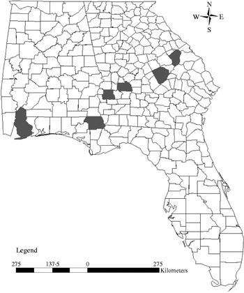
Winter wheat growth, development and yield as a function of weather and soil conditions, crop management and local genetics were simulated with the CSM-CERES-Wheat model (Ritchie et al. Reference Ritchie, Singh, Godwin, Bowen, Tsuji, Hoogenboom and Thornton1998) as included in the Decision Support System for Agrotechnology Transfer (DSSAT) v.4.5 (Hoogenboom et al. Reference Hoogenboom, Jones, Wilkens, Porter, Hunt, Boote, Singh, Uryasev, Lizaso, White, Ogoshi, Gijsman, Batchelor and Tsuji2009). The simulations were conducted for six counties in the south-eastern USA: Baldwin County, Alabama; Jackson County, Florida; and Jefferson, Laurens, Randolph and Sumter Counties, Georgia (Fig. 1). These counties are all among the top winter wheat production counties within the region (United States Department of Agriculture: National Agricultural Statistics Service 2009) and represent different climate (SERCC 2009) and soil conditions (Soil Survey Staff 2009). The simulations were conducted in the seasonal analysis mode (Thornton & Hoogenboom Reference Thornton and Hoogenboom1994) of DSSAT v.4.5. Weather data representing 67 growing seasons from 1939/40–2005/06 were included in the simulations to determine the impact of inter-annual weather variability. Weather input data for the simulation were obtained from the Cooperative Observer Program (COOP) network of the National Climatic Data Center (NCDC) with solar radiation estimated by the WGENR generator (Hodges et al. Reference Hodges, French and LeDuc1985) and adjusted to represent the south-eastern USA (Garcia y Garcia & Hoogenboom Reference Garcia y Garcia and Hoogenboom2005). Soil profile data for the simulated counties were obtained from the United States Department of Agriculture: Natural Resources Conservation Service (Soil Survey Staff 2009). Wheat production was simulated for the three most common cropland soils within each county. The two local winter wheat cultivars used were AGS 2000 and Pioneer 26R61. The crop management scenarios represented the recommended practices for the south-eastern USA (Lee et al. Reference Lee, Buntin, Culpepper, Harris, Martinez and Smith2008). Planting date was set to November 20. Row distance was 180 mm and the population was 405 plants/m2 at planting; the preceding crop was soybean. Nitrogen, in the form of ammonium nitrate, was broadcast at a rate of 34 kg/ha at planting and 45 kg/ha on February 15, when the crop was at the tillering stage. In the simulations, an additional nitrogen residue effect of 35 kg/ha from the preceding soybean crop was also included.
Simulated wheat production in Baldwin County, Alabama, Jackson County, Florida, and Jefferson, Laurens, Randolph and Sumter County, Georgia, USA (grey).

Wheat cultivar characteristics
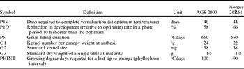
The cultivar coefficients for the wheat varieties AGS 2000 and Pioneer 26R61 were obtained from the USA Georgia Statewide Variety Trials data (Day et al. Reference Day, Coy and Rose2001; Rose et al. Reference Rose, Day, Coy and Lee2003, Reference Rose, Day and Coy2004, Reference Rose, Day and Coy2005) and from published cultivar information (United States Department of Agriculture: Soft Wheat Quality Laboratory 2001; Johnson et al. Reference Johnson, Barnett, Cunfer, Buntin and Bland2002). The parameters were calibrated with data collected during the 2002/03 growing season in Williamson, Georgia and evaluated with data collected during the 2000/01 growing season in Tifton, Georgia and during the 2003/04 growing season in Williamson. These sets of experimental data were selected because they reported straw yield, while the Georgia Statewide Variety Trial reports from other locations and growing seasons did not. Simulated grain yield was also evaluated against observed grain yield from Williamson in 2004/05. Daily weather data, including air temperature, rainfall and solar radiation, for the field trial locations were obtained from the Georgia Automated Environmental Monitoring Network (2009) . Soil data were obtained from the United States Department of Agriculture: Natural Resources Conservation Service (Soil Survey Staff 2009). The starting set of coefficients for both cultivars was the standard US winter wheat as included in the DSSAT v.4.5 package. Crop phenology parameters (Table 1) were changed to simulate observed anthesis and maturity date. Subsequently, parameters determining grain yield were calibrated. The parameter G2, which determines individual grain weight (mg), was set to 38 mg for AGS 2000, in accordance with Johnson et al. (Reference Johnson, Barnett, Cunfer, Buntin and Bland2002) . For Pioneer 26R61, G2 was set to 39 mg because it has a slightly larger kernel size than AGS 2000 (United States Department of Agriculture: Soft Wheat Quality Laboratory 2001). Finally, the remaining parameters that determine grain yield were adjusted to match the observed grain and straw yield.
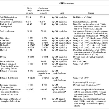
GHG emissions and sequestration in the wheat–ethanol production chain and emissions that could be replaced throughout the wheat–ethanol production chain

* In the straw- and grain-ethanol scenario, the GHG emissions that can be reduced by the use of co-products as animal feedstock depend on the grain/straw harvest ratio, which varies due to environmental conditions.
† The total avoided emissions depend on the grain/straw harvest ratio, which varies due to environmental conditions.
DM, dry matter.
Net reduction in GHG emissions
The reduction in GHG emissions was calculated separately for each of the six counties that were included in the study for the grain only scenario and for the grain and straw scenario. In order to determine and compare the climate change impact for different types of GHG, it is standard procedure to express emissions of all GHG in CO2-equivalents (CO2-equiv; IPCC 2006). In the present study, the following conversion factors were adopted: the GHG carbon dioxide (CO2), which was defined as having a climate change impact of 1 CO2-equiv; methane, which was set to a climate impact of 25 CO2-equiv; and nitrous oxide (N2O), which was set to a climate change impact of 298 CO2-equiv according to IPCC (2006) . The reduction in GHG emissions (CO2-equiv) was expressed as /km bio-ethanol use in a personal vehicle. This unit has been used in several previous studies of bio-ethanol (Tan & Culaba Reference Tan and Culaba2002; Quirin et al. Reference Quirin, Gartner, Pehnt and Reinhardt2004; Sheehan et al. Reference Sheehan, Aden, Paustian, Killian, Brenner, Walsh and Nelson2004). The unit of CO2 equiv/km was used because it facilitates a direct comparison of biofuel use with the use of fossil gasoline (Quirin et al. Reference Quirin, Gartner, Pehnt and Reinhardt2004). If another unit such as CO2 equiv/l ethanol or CO2 equiv/MJ had been used, the differences in fuel efficiency and energy content between ethanol and gasoline would first have to be accounted for to be able to compare these two types of fuels. The conversion to CO2 equiv/km was carried out by applying the following three-step procedure. In Step 1, the simulated wheat grain was converted into ethanol according to

where Y ethanol grain is the grain-ethanol (litre) that was produced, f grain is the grain-ethanol conversion factor (litre ethanol/kg dry matter (DM) wheat grain) and Y grain is the grain yield (kg DM/ha) that was simulated with the CSM-CERES-Wheat model. Similarly, the simulated straw yield was converted to cellulosic ethanol according to

where Y ethanol straw is the amount of ethanol (litre) that could be produced from straw (kg DM), f straw is the factor (litre/kg DM) to convert ethanol from straw, Y straw simul is the straw yield (kg DM/ha) that was simulated with CSM-CERES-Wheat and h straw is the fraction of the total straw yield that could be collected for ethanol use. This fraction was set to 0·87 of the total straw biomass, based on a straw height of c. 1 m for AGS 2000 and Pioneer 26R61 (Lee et al. Reference Lee, Buntin, Culpepper, Harris, Martinez and Smith2008) and a stubble height of 0·13 m, which is normal in wheat–soybean crop rotations in the south-eastern USA (Ferguson et al. Reference Ferguson, Lanclos, Leonard, Boquet, Hollier and Vidrine2008). For each county, the grain and straw yields from the CSM-CERES-Wheat simulations, which were used as inputs, were the weighted averages of the simulated grain and straw yields, respectively, for the 67 growing seasons. This procedure was included in the study to account for the temporal weather variation within the south-eastern USA. Moreover, in each county there were three sets of grain and straw yield simulations, representing the three most common cropland soil types. Prior to the GHG emission calculations, weighted average yields were calculated according to the relative fraction of each soil in the respective county. The weighted average grain and straw yield thus represented typical soil conditions for each county.
Step 2 of the calculations was conducted to determine the reduction in GHG emission/l bio-ethanol that was used in a flex-fuel vehicle as a replacement for gasoline. This procedure was calculated separately for ethanol obtained from grain and straw feedstock based on the following equation:

where E red L are reductions in GHG emissions in CO2 equiv/l ethanol, E avoid gas (CO2 equiv/l) represents the emissions that were avoided from the replaced gasoline, E avoid co-prod (CO2 equiv/l) represents the emissions that were avoided from the co-product replacements and E crop, E trp, E proc and E distr (CO2 equiv/l) are emissions that were related to wheat cropping, feedstock transportation, ethanol processing and ethanol distribution, respectively. The first two steps of this conversion procedure require separate calculations for ethanol obtained from either grain or straw feedstock due to different input values (see below for details). For the grain and straw scenario, the reductions in GHG emissions could subsequently be determined by weighing in the emissions related to grain-ethanol and straw-ethanol according to the grain-ethanol/straw-ethanol ratio. In Step 3, the reductions in GHG emissions were converted to CO2 equiv/km (E red km) use according to

where V eth fuel efficiency is the fuel efficiency (km/l) of E85 fuel use in a flex-fuel personal vehicle. This step is identical for ethanol obtained from both grain and straw. A description about how this procedure was applied in the two scenarios that were included in the present study is presented below.
GHG emissions from wheat cropping
The calculation of reduction in GHG emissions based on wheat production as a biofuel feedstock took into account emissions related to soil preparation, planting, fertilizer and pesticide applications, harvest and drying. Details of these emissions were obtained from the literature references (see Table 1) and adjusted to represent crop management practices, transportation distances and ethanol processing techniques in the south-eastern USA. GHG emissions in upstream activities, including fuel, fertilizer and pesticide production and transportation were also taken into account. In addition to direct emissions from farm operations, wheat cropping affects GHG emissions through its impact on soil carbon and nitrogen turnover, which in turn impacts net CO2 and N2O emissions (Franzluebbers et al. Reference Franzluebbers, Hons and Zuberer1998; Vinten et al. Reference Vinten, Ball, O'Sullivan and Henshall2002; De Klein et al. Reference De Klein, Novoa, Ogle, Smith, Rochette, Wirth, McConkey, Mosier, Rypdal, Eggleston, Buendia, Miwa, Ngara and Tanabe2006). The impact of changes in soil carbon pools on GHG emissions was calculated to represent wheat cropping in the south-eastern USA. It was assumed that a fraction of 0·50 of the winter wheat production for ethanol would replace winter fallow and that the other half of the production would replace non-ethanol winter wheat production. Statistics from the United States Department of Agriculture: National Agricultural Statistics Service (2004, 2009) indicate that there are large areas of cropland that are now left fallow during the winter season, with potential for winter wheat production. From a field study in eastern Texas in the south-central USA with similar climate and soil conditions and a similar land use history as in the south-eastern USA, a net increase of soil carbon content of 0·43 kg/m2 was reported 9 years after the crop rotation was changed from soybean/winter fallow to soybean/winter wheat (Franzluebbers et al. Reference Franzluebbers, Hons and Zuberer1998). This improved carbon sequestration was considered to be representative for this particular change of crop rotation. Thus, the wheat-ethanol was credited with a reduction of GHG that was equal to a fraction of 0·50 of the average annual rate of the sequestered carbon reported by Franzluebbers et al. (Reference Franzluebbers, Hons and Zuberer1998), making these assumptions more general for cropping systems in the south-eastern USA. The impact of replacing peanut–winter fallow, which is another common crop rotation in the south-eastern USA, with peanut–winter wheat could have a similar impact on the soil carbon stocks, as was found by Franzluebbers et al. (Reference Franzluebbers, Hons and Zuberer1998) . Peanut and soybean are both leguminous crops and normally produce similar amounts of biomass per area. Thus, the calculations should also be representative for a generic crop rotation that represents conditions for the south-eastern USA. The 0·50 fraction of winter wheat production in the two scenarios of the present study that replaced non-ethanol winter wheat did not entail any change in crop rotation. Therefore, it was assumed that, for this fraction, the soil carbon was in steady state and that no net change in soil carbon would occur, according to Franzluebbers (Reference Franzluebbers2005) .
In both scenarios, it was assumed that the straw was removed from the field, which is a common practice in winter wheat production in the south-eastern USA (Lee et al. Reference Lee, Buntin, Culpepper, Harris, Martinez and Smith2008). In the grain only scenario, the straw was used for purposes other than ethanol production. For the 0·50 fraction of the ethanol wheat production that replaced non-ethanol winter wheat, this practice did not entail any change in crop management. However, in the grain only scenario, the straw from the 0·50 fraction of winter wheat that replaced winter fallow could replace straw yield from another wheat field. Given the same straw production and farm operation machinery, this straw removal would lead to a replacement of the same amount of GHG emissions related to the straw collection. However, the potential impact on soil carbon stock due to this possible change in straw collection management in other fields where the straw was not collected after harvest was not taken into account in the calculations. It is rather difficult to estimate the potential impact of modifications in the harvest management of straw. The impact of cereal crop residue management on soil carbon content has differed among studies under various conditions (Silgram & Chambers Reference Silgram and Chambers2002; Wilhelm et al. Reference Wilhelm, Johnson, Hatfield, Voorhees and Linden2004).
Soil N2O emissions were estimated according to the IPCC (2006) guidelines for non-organic soils, which were assumed to be representative for the south-eastern USA. These emissions were affected by the amount of N fertilizer that was applied and the amount of above- and below-ground wheat residues that were left on the field after harvest; they were set to 0·0157 kg/kg N that was applied in the fertilizers or remaining in the wheat residues, according to the IPCC (De Klein et al. Reference De Klein, Novoa, Ogle, Smith, Rochette, Wirth, McConkey, Mosier, Rypdal, Eggleston, Buendia, Miwa, Ngara and Tanabe2006). The N fraction of above- and below-ground wheat residues remaining after wheat harvest were set to a fraction of 0·006 and 0·009 of total DM, respectively (De Klein et al. Reference De Klein, Novoa, Ogle, Smith, Rochette, Wirth, McConkey, Mosier, Rypdal, Eggleston, Buendia, Miwa, Ngara and Tanabe2006). The remaining residues of the preceding soybeans were not taken into account since this crop was not affected by the ethanol production. The below-ground biomass used to calculate the nitrous oxide emissions was input from the CSM-CERES-Wheat model and represented the maximum below-ground biomass during the growing season.
GHG emissions from transportation, and ethanol processing and distribution
It was assumed for the present study that all ethanol was processed in Camilla, Mitchell County, Georgia, where a dry mill maize-based ethanol plant is currently in operation (First United Ethanol 2010). However, at the time of writing this paper there is no wheat-based bio-ethanol processing facility in operation in the south-eastern USA, but the dry mill processing of maize-ethanol and wheat-ethanol from grain feedstock is very similar (S&T2 Consultants 2003). Therefore, the use of wheat grain feedstock instead of maize would not require any major processing changes. For processing of straw into bio-ethanol, a commercial-scale production at the same site was assumed, based on future projections for this type of ethanol feedstock (Sheehan et al. Reference Sheehan, Aden, Paustian, Killian, Brenner, Walsh and Nelson2004; Lavigne & Powers Reference Lavigne and Powers2007). Ideas to add cellulosic feedstock for bio-ethanol production facilities in the south-eastern USA have been expressed (Robertson Reference Robertson2008). The conversion factor for grain-ethanol was set to 428 litres ethanol/tonne DM by using standard processing techniques currently in use for wheat-ethanol production ((S&T)2 Consultants 2003). The conversion factor for straw-ethanol was set to 250 litres ethanol/tonne DM (Bernesson & Nilsson Reference Bernesson and Nilsson2005). The latter conversion factor assumes processing of ethanol from cellulosic material based on projected large-scale cellulosic ethanol production. However, it should be noted that ethanol processing from cellulosic material at the present time only exists at a pilot or experimental scale.
The present study assumed that all wheat grain and straw were transported by truck from the field in the respective county to the ethanol processing plant in Camilla, Georgia. The diesel consumption was set to 2·07 km/l, for a grain loading capacity of 13 600 kg wheat grain with a moisture content of 0·14 (Wang et al. Reference Wang, Wu and Huo2007). It was assumed that the same truck type with the same loading capacity was used for the transportation of straw and that the moisture content of the straw was the same as that for grain, i.e. 0·14. GHG emissions due to the transportation of feedstock including emissions related to the upstream production of the transportation fuel were calculated with data from the IPCC (Waldron et al. Reference Waldron, Harnisch, Lucon, Mckibbon, Saile, Wagner, Walsh, Eggleston, Buendia, Miwa, Ngara and Tanabe2006). The GHG emissions due to transportation were calculated separately for each county that was considered in the present study. The transportation distance was set equal to the distance from the geographic centre of each county to the ethanol processing plant in Camilla, Mitchell County, Georgia. For grain-ethanol processing in Camilla, natural gas is the main energy source and electricity is a smaller part of the total energy use (First United Ethanol 2010). Therefore, the same emissions as those that have been calculated in Canada for wheat-ethanol processing in natural gas-based wheat grain-ethanol production were assumed ((S&T)2 Consultants 2003). For the straw-ethanol processing there were no GHG emissions, as based on projected cellulosic ethanol processing. In this type of process, no requirements of fossil fuel energy are projected. The lignin fraction of the wheat straw, which cannot be converted into ethanol, will instead be used as a feedstock to cover the processing energy requirements. In addition, an electricity surplus for use outside the ethanol processing facility will be generated (Sheehan et al. Reference Sheehan, Aden, Paustian, Killian, Brenner, Walsh and Nelson2004; Lavigne & Powers Reference Lavigne and Powers2007). GHG emissions from the distribution of ethanol from the processing facility to the gas station were set to the average for ethanol distribution for personal vehicle use in the USA, as previously assessed by Wang et al. (Reference Wang, Wu and Huo2007) .
Reductions in GHG emissions
The ethanol that was produced in both scenarios was used in the form of E85. The fuel was used in a flex-fuel model of the Chevrolet Impala make, which is a typical flex-fuel personal vehicle for the US market. A flex-fuel vehicle can use either E85 or regular gasoline as fuel. The flex-fuel Chevrolet Impala has a gasoline efficiency of 9·76 km/l and an E85 efficiency of 7·48 km/l with 0·55 of that accounted for by city use and 0·45 by highway use (United States Department of Energy 2009). GHG emissions for the replaced gasoline and emissions for 0·15 gasoline fraction in the E85 fuel in this vehicle model were calculated with the GREET model v.1.8 as set for typical US gasoline production (Wang et al. Reference Wang, Wu and Huo2007).
Distillers' dry grain with solubles (DDGS) was produced as a co-product from the grain-ethanol processing. The DDGS could replace 1·0 kg of maize and 1·04 kg of soybean meal ((S&T)2 Consultants 2003). The replaced GHG emissions were those that were required for the production of the replaced feedstock (Hill et al. Reference Hill, Nelson, Tilman, Polasky and Tiffany2006). As mentioned above, the surplus electricity that is generated from the straw-ethanol process can be used outside the ethanol processing facility (Sheehan et al. Reference Sheehan, Aden, Paustian, Killian, Brenner, Walsh and Nelson2004; Lavigne & Powers Reference Lavigne and Powers2007). In the present study, the electricity surplus generation ratio was set at 1·95 MJ/l cellulosic ethanol. This ratio has been estimated for future maize stover ethanol production (Sheehan et al. Reference Sheehan, Aden, Paustian, Killian, Brenner, Walsh and Nelson2004), which would be similar to wheat straw-ethanol production. The electricity, and associated GHG emissions, that could be replaced by the processing electricity surplus was assumed to consist of electricity that was generated from different types of power plants according to their respective share of the total electricity production in the states of Alabama, Florida and Georgia in 2007 (Energy Information Administration 2009).
Statistical analysis
To determine whether there were any differences in grain and straw yields among the locations, as well as differences in reductions in GHG emissions between the two scenarios and among locations, an analysis of variance (ANOVA) was conducted. Each growing season was considered as a replicate. The PROC GLM of SAS (SAS Institute Inc. 2002) was used for this statistical analysis.
RESULTS
Model calibration and evaluation
The cultivar-specific coefficients of the CSM-CERES-Wheat model were calibrated by using a set of cultivar coefficients that first minimized the difference between simulated and observed days of anthesis and maturity, respectively, for the winter wheat variety trial in Williamson, Georgia in 2002/03. Subsequently, the relative difference between simulated and observed grain yields and above-ground biomass for the same growing season was minimized. These calibration procedures followed the guidelines by Boote (Reference Boote, Hoogenboom, Wilkens and Tsuji1999) . The calibrated specific parameters for the two cultivars AGS 2000 and Pioneer 26R61 are presented in Table 2. The differences between simulated and observed anthesis and maturity days were 3 days or less, which is within the range of uncertainty for the observations. Simulated grain DM yield was <4% higher than observed values. For above-ground biomass, simulated values were 7% higher than observed values in AGS 2000, whereas for Pioneer 26R61, the simulated values were 31% lower than observed values. This relatively poor above-ground biomass prediction could be related partly to the uncertain above-ground biomass observations as indicated by an unrealistically high harvest index (HI; defined as the proportion of the grain yield to the total above-ground biomass; Hay Reference Hay1995). Normally, the HI of wheat ranges from 0·4 to 0·6 (Hay Reference Hay1995). The observed HI for Pioneer 26R61 (variety trial conducted in Williamson during the 2002/03 season) was 0·70.
Cultivar-specific coefficients of the CSM-CERES-Wheat model for the winter wheat varieties AGS 2000 and Pioneer 26R61 in the CSM-CERES-Wheat model

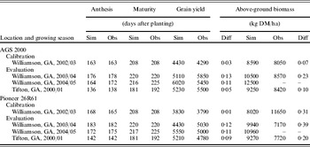
Following calibration, the CSM-CERES-Wheat model was evaluated for variety trials that were conducted in Tifton, Georgia, for the growing season of 2000/01 and in Williamson, Georgia for the growing seasons of 2003/04 and 2004/05. Model evaluation showed that there was a difference of 2–8 days between simulated and observed anthesis dates for AGS 2000 and 0–3 days for Pioneer 26R61. There was a difference of 0–11 days between simulated and observed maturity dates for both cultivars. The model also predicted the observed grain yield well; the difference between simulated and observed grain yields ranged from 4·8 to 12·6%. The differences between simulated and observed above-ground biomass were relatively greater than the differences between simulated and observed grain yield (Table 3). With respect to the evaluation of Pioneer 26R61, the relatively poor above-ground yield predictions for Williamson in 2003/04 could be related to uncertainties in the above-ground yield observations, as indicated by unrealistically high harvest indices of 0·67 and 0·69 for AGS 2000 and Pioneer 26R61, respectively.
Simulated and observed, anthesis and maturity dates and grain and straw DM yield in the CSM-CERES-Wheat model evaluation

Sim, simulated; Obs, observed; Diff, difference, DM, dry matter.
Simulated grain and straw yield for the six counties
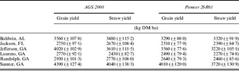
Yield for grain and straw differed significantly among the six counties for which wheat production was simulated. Across all simulated years and for both cultivars, the highest grain and straw yield was found in Sumter County, Georgia, while Laurens County, Georgia had the lowest average grain and straw yield (Table 4). There was also a large variation in grain and straw yields among simulation years and within counties as a result of inter-annual weather variability. For example, the total precipitation during the growing season varied substantially among the years of simulation (data not shown). Moreover, the intra-seasonal temporal distribution of rainfall with respect to crop requirements could have affected both grain and straw yield.
Average simulated winter wheat grain and straw yield (±s.e.m.) for six counties in the south-eastern USA

DM, dry matter.
Reduction in GHG emissions
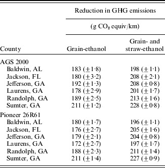
The differences in grain and straw yield among the locations and the years affected the reduction in GHG emissions for the two scenarios where bio-ethanol from the winter wheat feedstock replaced gasoline in a personal flex-fuel vehicle. For the grain only scenario, the reduction in GHG emissions from substituting gasoline with wheat-ethanol was 187 g CO2 equiv/km, as averaged across all counties, all years and both cultivars. The substitution of gasoline with ethanol from both grain and straw for the second scenario, as averaged across all counties, years and both cultivars, resulted in a reduction in GHG emissions by 208 g CO2 equiv/km. This was a significantly (P<0·001) larger reduction than for the substitution with ethanol produced from only grain feedstock. Also, within each county the average reduction in GHG emissions across all growing seasons was significantly higher (P<0·001) for the grain and straw scenario than for the grain only scenario for both cultivars.
Within the grain only, and the grain and straw scenarios, respectively, the wheat production location impacted the potential reduction in GHG emissions. Averaged for the two cultivars and all years, the reductions in GHG emissions were, in both scenarios, largest when the ethanol was processed from wheat that was produced in Sumter County, Georgia (211 g CO2 equiv/km for the grain only scenario and 228 g CO2 equiv/km for the grain and straw scenario). Bio-ethanol produced from wheat that was grown in Laurens County, Georgia, resulted in the lowest reduction in GHG emissions for the grain only scenario (175 g CO2 equiv/km) and from wheat production in Baldwin County, Alabama, for the grain and straw scenario (197 g CO2 equiv/km) as averaged for the two cultivars. For each cultivar analysed separately, the reduction in GHG emissions was largest for Sumter County, Georgia for both scenarios. For the grain only scenario, reductions in GHG emissions were, for both cultivars, smallest for Laurens County, Georgia. For the grain and straw scenario the GHG emissions were smallest for Baldwin County, Alabama for both cultivars (Table 5).
Average reduction in GHG emissions (±s.e.m.) for the two scenarios where gasoline was replaced by ethanol from grain only and ethanol from both grain and straw

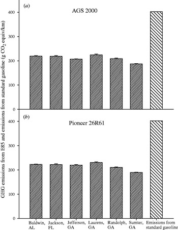
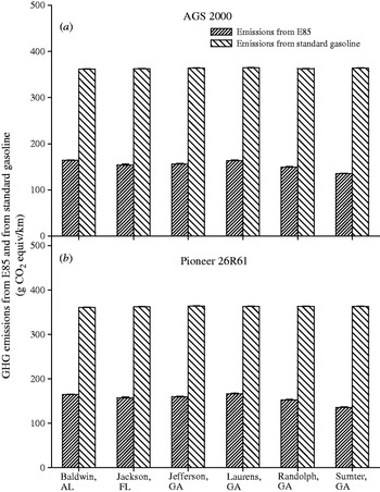
In the grain only scenario, the total GHG emissions that were associated with E85 use and production represented 0·43–0·52 of GHG that would have been emitted if standard gasoline had been used. The total emissions from the E85 include emissions in the entire ethanol production chain as well as emissions related to the gasoline fraction of the E85 fuel. The relative reductions in GHG emissions from E85 use were largest in Sumter County, Georgia and smallest in Laurens County, Georgia for both cultivars (Fig. 2). For the grain- and straw-ethanol scenario, the total emissions associated with the E85 represented between 0·54 (Baldwin County) and 0·62 (Sumter County) of the overall emission from standard or fossil-fuel based gasoline use in the flex-fuel vehicle (Fig. 3). The total emissions that could be avoided from the replacement of the standard gasoline in the grain and straw scenario varied slightly among locations (Fig. 3) and years. The reason for this variation was a varying grain/straw ratio and the fact that larger amounts of GHG emissions could be replaced when the straw-ethanol was used than when grain-ethanol was used. The latter was in turn due to the fact that more GHG emissions could be replaced by the electricity that was generated in the straw-ethanol production than by the animal feed that was generated from the grain-ethanol production.
Greenhouse gas (GHG) emissions related to E85 production of which the ethanol part is processed from wheat grain (grain only scenario), AGS 2000 (a) and Pioneer 26R61 (b), and corresponding emissions related to standard gasoline production and use (error bars indicate s.e.m.).

GHG emissions related to E85 production of which the ethanol part is processed from both grain- and straw-ethanol (grain and straw scenario), AGS 2000 (a) and Pioneer 26R61 (b), and corresponding emissions related to standard gasoline production and use (error bars indicate s.e.m.).

Impact of inter-annual weather variability on GHG emissions
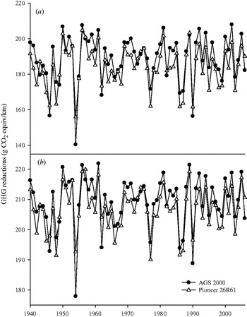
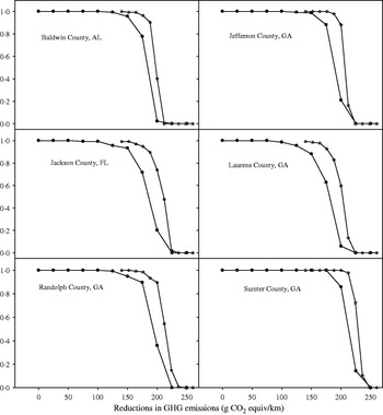
The reduction in GHG emissions varied substantially for both the grain only and the grain and straw scenarios due to inter-annual weather variability. Across all wheat production locations and for all cultivars, the variation in the reduction in GHG emissions among growing seasons was, on average, 156–205 g CO2 equiv/km for the grain only scenario. For the grain and straw scenario, the variation in the reduction in GHG emissions ranged from 190 to 220 g CO2 equiv/km (Fig. 4) as averaged across locations and for both cultivars. For a few of the locations, the inter-annual variation in the reduction in GHG emissions was even more pronounced (data not shown). A small reduction in GHG emissions due to low yield generally occurred during growing seasons that had lower precipitation than normal or when the temporal inter-seasonal rainfall pattern was unfavourable with respect to crop need (data not shown). Nevertheless, across the two cultivars, there was a net reduction in GHG emissions for all the years for both the grain only scenario and the grain and straw scenario (Fig. 5). In addition, the difference between the two cultivars in the net reduction in GHG emissions was always relatively small for all years (data not shown).
The inter-annual variation in GHG reductions from wheat-ethanol use due to temporal weather variability: feedstock from grain (a) and feedstock from grain and straw (b).

Cumulative distribution functions of GHG emissions average of two cultivars for six locations: the grain only scenario (circle) and the grain and straw scenario (star).

DISCUSSION
The present study shows that there is potential for decreasing GHG emissions by replacing regular gasoline from fossil fuel with bio-ethanol from winter wheat that is produced in the south-eastern USA. These results confirm the reductions in GHG emissions that have been shown for ethanol produced from wheat feedstock grown under different conditions in other parts of the world including Europe (Bernesson et al. Reference Bernesson, Nilsson and Hansson2006; Gabrielle & Gagnaire Reference Gabrielle and Gagnaire2008; Rettenmaier et al. Reference Rettenmaier, Reinhardt, Gartner and Von Falkenstein2008; Borjesson Reference Borjesson2009) and Canada ((S&T)2 Consultants 2003). From the perspective of bio-ethanol production in the USA, it is also relevant to compare the results with the reduction in GHG emissions through the use of maize-ethanol. Maize is currently the feedstock for more than 0·90 of all bio-ethanol produced in the USA (Renewable Fuels Association 2010). The reduction in GHG emissions found in the present study ranged from 43 to 62% compared to standard gasoline use and was also larger than the corresponding reduction in GHG emissions from the use of maize-ethanol in the USA, which normally ranges from 15 to 24% (Farrell et al. Reference Farrell, Plevin, Turner, Jones, O'Hare and Kammen2006; Wang et al. Reference Wang, Wu and Huo2007; Liska et al. Reference Liska, Yang, Bremer, Klopfenstein, Walters, Erickson and Cassman2009). Wheat grain and straw feedstock grown in the south-eastern USA has the potential to increase as a source for bio-ethanol production that could thus lead to a decrease in GHG emissions compared to the current situation of mainly maize-ethanol production and use. The results from the grain and straw scenario were especially promising when compared to maize-grain-ethanol production.
There was a substantial impact of inter-annual weather variability on the reduction in GHG emissions. Similarly, the difference in GHG emissions among the wheat-producing counties also indicated that the spatial climate and weather variability in the south-eastern USA are important factors that can affect GHG emissions. Gabrielle & Gagnaire (Reference Gabrielle and Gagnaire2008) determined the effect of local climate, weather and soil variability on ethanol produced from wheat grain and associated reductions in GHG emissions for conditions representing northern France. However, most other studies of GHG emissions and wheat-ethanol or other biofuels from the agricultural sector have not explicitly taken these factors into account. Nevertheless, knowledge about the potential influence of environmental conditions on biofuel production systems is critical in evaluating their potential and sustainability in the general context of GHG emissions and climate change. Therefore, simulation methodologies similar to those applied in the present study could also be used to determine the explicit impact of climate, weather and soil variability on other agricultural bioenergy production systems in different regions of the world. Moreover, future climate change partly due to GHG emissions from human activity could change the growth conditions for biofuel feedstock. Further research aimed at evaluating GHG emissions in biofuel production under different climate change scenarios would, therefore, increase the understanding of the role of biofuels in future energy systems.
A comparison of the systems that were studied in the present paper with other wheat-ethanol production systems provides an indication of how the south-eastern USA system could be improved. Naturally, the amount of GHG reduction from gasoline replacement with bio-ethanol from wheat feedstock is not only due to crop yield and management but also due to ethanol processing techniques (Rettenmaier et al. Reference Rettenmaier, Reinhardt, Gartner and Von Falkenstein2008; Borjesson Reference Borjesson2009). In the present study, for the grain only scenario, the emissions based on current natural gas use in the ethanol processing facility (First United Ethanol 2010) were estimated. However, a previous study showed that GHG emissions from the processing step of grain-based ethanol can be reduced by 90% if biomass in the form of forest chips is used for processing energy instead of natural gas (Borjesson Reference Borjesson2009). The south-eastern USA has large forest resources, unlike many other regions with a significant bio-ethanol production such as the mid-western USA. Use of these resources for ethanol processing energy would increase the benefits of bio-ethanol in the south-eastern USA from a GHG perspective.
In conclusion, the present study demonstrates that the use of winter wheat grown in the south-eastern USA as a source for bio-ethanol production can reduce GHG emissions. The reductions from the grain only scenario are comparable to wheat-ethanol production in other regions and are favourable compared to maize-ethanol from the mid-western USA. The large reductions in GHG emissions in the grain and straw scenario are promising given a successful development of cellulosic ethanol processing techniques. Wheat straw could be used as feedstock to meet the mandate of cellulosic ethanol use in the USA by 2022 as stated in the Energy Independence and Security Act of 2007 (US Congress 2007). Moreover, the results of the present study stress the importance of weather, climate and soil variability to the potential of using biofuels as a means of reducing GHG emissions. In future research, the crop simulation methods presented here could be further expanded. For example, applying a model of long-term soil carbon content as a response to climate and other environmental factors would enable a more refined assessment of climate and soil factors on GHG emissions from the agricultural biofuel production. The crop simulation approach of the present study could also be applied to assess the impact of climate, weather and soil variability on other biofuel feedstocks and other agricultural production regions. Likewise, evaluations under climate change scenarios would be of high societal interest in the context of GHG emissions in general.
This work was conducted under the auspices of the Southeast Climate Consortium (SECC; www.SEClimate.org) and supported by a partnership with the United States Department of Agriculture – Risk Management Agency (USDA-RMA), by grants from the US National Oceanic and Atmospheric Administration – Climate Program Office (NOAA-CPO) and USDA Cooperative State Research, Education and Extension Services (USDA – National Institute of Food and Agriculture) and by State and Federal funds allocated to Georgia Agricultural Experiment Stations Hatch project GEO01179.