1 Introduction
Multi-instance (MI) learning (Dietterich et al., Reference Dietterich, Lathrop and Lozano-Pérez1997; also known as ‘multiple-instance learning’) is a variant of inductive machine learning that has received a considerable amount of attention due to both its theoretical interest and its applicability to real-world problems such as drug activity prediction and image classification.
MI learning, as it is commonly defined, belongs to the supervised learning paradigm, which aims to solve classification and regression problems by using algorithms to build models from data based on a set of labeled examples. The majority of the work in MI learning is concerned with binary classification problems, where each example has a classification label that assigns it into one of two categories—‘positive’ or ‘negative’. The goal is to ‘learn’ a model based on the training examples that is effective in predicting the classification labels of future examples. All training examples have been (often manually) assigned a class label, which is why the term supervised learning is used.
Where MI learning differs from the traditional scenario is in the nature of the learning examples. In the traditional supervised learning scenario, each example is represented by a fixed-length vector of features. However, in MI learning each example is represented by a multi-set (or bag, as computer scientists often call it) of feature vectors. In other words, each example contains one or more feature vectors. The feature vectors are referred to as instances. Classification labels are only provided for entire bags, and the task is to learn a model that predicts the classification labels for unseen future bags.Footnote 1
In early MI research, a strong assumption was made regarding the relationship between instances inside the bags and the label of the bag. This assumption is generally referred to as the standard MI assumption. Under this assumption, each instance has a hidden class label that identifies it as either a positive or a negative instance, and a bag is considered to be positive if and only if it contains at least one positive instance. This is generally believed to be true for the musk drug activity prediction problem, where a molecule will have the desired drug effect if and only if one or more of its conformations binds to the target binding site (Dietterich et al., Reference Dietterich, Lathrop and Lozano-Pérez1997). However, in other problem domains this assumption may not apply, and different or more general assumptions may be needed. A significant amount of the more recent research in MI is concerned with cases where the standard view of MI learning is relaxed, and alternative assumptions are used instead.
Unfortunately, it is often not clear what particular assumptions are used and how they relate to other assumptions from the literature. This is perhaps at least partially due to the fact that the use of the term ‘MI learning’ has evolved from the original statement by Dietterich et al. (Reference Dietterich, Lathrop and Lozano-Pérez1997). Dietterich et al. included the standard MI assumption in their original definition of MI learning, but many authors now include alternative assumptions within the MI learning framework (see, e.g. Xu, Reference Xu2003; Chen et al., Reference Chen, Bi and Wang2006; Dong, Reference Dong2006). To compound the issue, some authors use alternative MI assumptions without explicitly describing the assumptions used. In this paper, we aim to shed some light on existing MI assumptions and relationships by reviewing the MI assumptions that can be found in the literature. This paper is not intended as a review of algorithms for MI learning that implement the standard MI assumption.
2 Background
This section gives an overview of machine learning, with emphasis on supervised learning and the MI learning scenario. MI learning is defined, and the motivations for it are explained.
2.1 Machine learning
Every day, we as humans discover new facts about our world. We interact with the environment around us, and receive feedback through our empirical faculties—our senses. We are able to recognize trends and can begin to anticipate the consequences of our actions. The process that allows us to do this is called learning. It is ubiquitous and most of us take it for granted.
Learning is a task that is normally associated with humans (and intelligent non-human animals), hence the problem of creating machines that can learn falls within the umbrella of artificial intelligence. While the creation of truly ‘intelligent’ machines still seems to be a long way off, machine learning as a practical discipline is a success story of modern artificial intelligence. Many algorithms have been discovered that allow machines to make inferences from observed data, effectively ‘learning’ non-trivial facts and behaviors.
Under the guise of data mining, these algorithms have many commercial applications. Machines are far more efficient and reliable than humans at processing large amounts of data. For this reason, learning algorithms can offer huge cost saving and efficiency benefits to businesses, and have successful applications in many domains from medicine to marketing.
2.2 Supervised learning
Supervised learning is the branch of machine learning that is concerned with algorithms that can learn concepts from labeled examples. As an input, the algorithm requires a set of example cases, each of which has been given a label corresponding to some important property of the example. The task of the algorithm is to build a model that will generate accurate predictions of the labels of future examples.
Let us illustrate this with a simple example. Suppose that we are amateur botanists, and we wish to learn to distinguish between instances of the various species of the iris genus of flowering plants. An expert has given us a set of examples of some of the species of the genus. Once we have seen a few examples of each, we can attempt to infer the defining characteristics of each species. Once we have discovered the pattern, we can become proficient at labeling arbitrary iris plants.
Having introduced the subject and its terminology via a simple example, we may now formally define the standard supervised machine-learning scenario. An instance is a vector of N features concatenated with a class label, of the form {x | g(x)}, where x = {x 1, x 2,…, xN} is the feature vector and g(x) is the label of the instance. Features and class labels are typically either elements of the real numbers (numeric attributes) or domain-specific sets of names (nominal attributes).
The task is to find g(x), based on a given labeled set of instances, where the labels have been assigned based on g(x). When the class is a nominal attribute, this process is called classification. When the class is a numeric attribute, the process is called regression.
The underlying classification process g(x) is known in machine learning terminology as a concept. The g(x) may be either a function or a non-deterministic process. Given a set of training examples to learn from, a supervised machine learning algorithm outputs a model that is intended to be a best-guess approximation to g(x). Such a model is known as a concept description.
This paper is about a variation of standard (single-instance) supervised learning called MI learning.
2.3 MI Learning
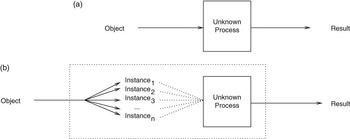
MI learning, as defined by Dietterich et al. (Reference Dietterich, Lathrop and Lozano-Pérez1997), is a variation on the standard supervised machine learning scenario. In MI learning, each example consists of a multi-set (bag) of instances. Each bag has a class label, but the instances themselves are not explicitly labeled. The learning problem is to build a model based on given example bags that can accurately predict the class labels of future bags. The difference between standard supervised learning and MI learning is illustrated in Figure 1.
(a) The traditional supervised machine-learning scenario. (b) Multi-instance learning. Figure based on a similar diagram by Dietterich et al. (Reference Dietterich, Lathrop and Lozano-Pérez1997)

An example will once again help to illuminate the concept. Chevaleyre and Zucker (Reference Chevaleyre and Zucker2001) refer to this example as the simple jailer problem. Imagine that there is a locked door, and we have N key chains, each containing a bunch of keys. If a keychain (i.e. bag) contains a key (i.e. instance) that can unlock the door, that key chain is considered to be useful. The learning problem is to build a model that can predict whether a given key chain is useful or not.
2.3.1 Definition of MI learning
We now present a formal definition of the MI problem. This formalization is a refinement of those used by Weidmann et al. (Reference Weidmann, Frank and Pfahringer2003) and Gärtner et al. (Reference Gärtner, Flach, Kowalczyk and Smola2002). In this paper, we follow the trend established by the majority of the work in this field (a notable exception being Zhou & Zhang, Reference Zhou and Zhang2006) and assume a binary class attribute Ω = {+, −}. Let χ be the instance space. Then an MI concept is a function  . The task in MI learning is to learn this function, based on a number of example elements of the function.
Here,  refers to the set of all functions from χ to
 , which is isomorphic to the set of all multi-subsets of χ, viewing the output of
 as the number of occurrences of x in the multi-set. Such functions are known as multiplicity functions, and are a direct generalization of indicator functions for ordinary sets.
Note that this differs slightly from the formulation used by Weidmann et al., who define an MI concept as a function νMI : 2χ→Ω. Here, 2χ, the set of indicator functions over χ, is isomorphic to the power set of χ, but this does not take into account the fact that duplicate instances are allowed in a bag. Our alternative definition of an MI concept explicitly defines the problem examples as multi-sets rather than just sets. This is important for some generalized MI concepts.
2.4 The standard MI assumption
A large percentage of the work on MI learning, including all early works and notably Dietterich et al. (Reference Dietterich, Lathrop and Lozano-Pérez1997) and Maron and Lozano-Pérez (Reference Maron and Lozano-Pérez1997), makes a particular assumption regarding the relationship between the instances within a bag and the class label of the bag. Dietterich et al. considered this assumption to be so fundamentally important that they included it as part of their definition of MI learning. We will follow Weidmann et al. (Reference Weidmann, Frank and Pfahringer2003), and refer to this assumption as the standard MI assumption.
The standard MI assumption states that each instance has a hidden class label c∈Ω = {+, −}. Under this assumption, an example is positive if and only if one or more of its instances are positive. Thus, the bag-level class label is determined by the disjunction of the instance-level class labels.
Formally, let  be a bag containing n instances from feature space χ. Each instance has a class label determined by some process g : χ →Ω. Let
 be a standard MI concept, and equate ‘+’ with the logical constant ‘True’, and ‘−’ with the logical constant ‘False’. Then:

It should be noted that the standard MI assumption is asymmetric: if the positive and negative labels are reversed, the assumption has a different meaning. Therefore, when we apply this assumption, we need to be clear which label should be the positive one.
The standard MI assumption was adopted because it is believed to be appropriate for the musk problem domain. In the musk problem, it is assumed that a molecule (represented by a bag of instances) will emit a musky smell if and only if one of its conformations (represented by an individual instance) binds to a certain target site, hence the standard MI assumption applies (Dietterich et al., Reference Dietterich, Lathrop and Lozano-Pérez1997).
A number of learning algorithms for MI classification under the standard MI assumption have been proposed in the literature. Dietterich et al. (Reference Dietterich, Lathrop and Lozano-Pérez1997) presented several algorithms for learning axis-parallel rectangles to identify the positive region of instance space. A bag is classified as positive if it has at least one instance in this region. Maron and Lozano-Pérez (Reference Maron and Lozano-Pérez1997) defined diverse density, a measure of the likelihood that a point in instance space is a positive target concept, and used a gradient search to find the point that is most likely to define the target concept. A refinement of this algorithm, expectation maximization (EM)-diverse density (DD), was proposed by Zhang and Goldman (Reference Zhang and Goldman2001).
Several single instance learning methods have been ‘upgraded’ to the MI scenario under the standard MI assumption, including support vector machines (Andrews et al., Reference Andrews, Tsochantaridis and Hofmann2002), neural networks (Ramon & De Raedt, Reference Ramon and De Raedt2000) decision trees (Blockeel et al., Reference Blockeel, Page and Srinivasan2005), (Chevaleyre & Zucker, Reference Chevaleyre and Zucker2001), decision rules (Chevaleyre & Zucker, Reference Chevaleyre and Zucker2001) and weak learners for boosting (Auer & Ortner, Reference Auer and Ortner2004). Zhou and Xu (Reference Zhou and Xu2007) showed that MI learning under the standard MI assumption could be viewed as a semi-supervised learning problem with the additional constraint that positive bags must contain at least one positive instance. They adapted semi-supervised support vector machines to the standard MI scenario by encoding this ‘positive constraint’ in the objective function of the support vector machine (SVM).
2.5 Alternative Assumptions
As (at least in part) the inclusion of the standard MI assumption in Dietterich et al.’s (Reference Dietterich, Lathrop and Lozano-Pérez1997) definition of MI learning, it was initially adopted ubiquitously by the fledgeling MI learning community. In more recent years, there has been a trend toward the relaxation of this strict view of MI learning (Xu, Reference Xu2003).
When the standard MI assumption is relaxed, other interactions between instances and the class labels of bags are possible. We refer to such interactions as MI assumptions, since we must assume that such a relationship between bags and class labels occurs when we use a learning algorithm to build a predictive model. In order to make learning computationally feasible, it is generally necessary to reduce the hypothesis space by making use of some MI assumption.
Although many recent authors have (implicitly or explicitly) abandoned the standard assumption, it is often not precisely stated that new assumptions have been used (Xu, Reference Xu2003). Moreover, the literature is not in agreement on whether the relaxed version of the MI problem belongs within the umbrella of MI learning, or is a separate problem. Some authors, notably Weidmann et al. (Reference Weidmann, Frank and Pfahringer2003) and Scott et al. (Reference Scott, Zhang and Brown2005), refer to the relaxed MI scenario as generalized MI, while others, such as Xu (Reference Xu2003), Chen et al. (Reference Chen, Bi and Wang2006), Dong (Reference Dong2006) and Foulds (Reference Foulds2008), include alternative MI assumptions within the MI framework. In particular, Xu explicitly extends the definition of MI learning to include other assumptions.
We contend that the term ‘multi-instance learning’ should contrast directly with ‘single-instance learning’, and connotes any type of learning where several instances can be included within a single learning example, regardless of the assumptions used. Hence, we follow Xu, and use the term to refer to the relaxed version of MI learning as well as the standard MI scenario. We shall reserve the term ‘generalized MI learning’ to refer MI assumptions that are strictly more general than the standard assumption, such as those proposed by Weidmann et al. (Reference Weidmann, Frank and Pfahringer2003) and Scott et al. (Reference Scott, Zhang and Brown2005).
2.6 Motivations for alternative MI assumptions
Although the standard MI assumption is widely believed to be appropriate for the musk drug activity prediction problem, the MI representation can be applied to a number of other problem domains where the standard MI assumption may not be directly applicable. In these domains, algorithms that rely upon alternative MI assumptions may be more appropriate.
A prominent example of this is the task of learning visual concepts from databases of labeled images. This learning problem arises in several computer vision tasks including object detection or recognition, image categorization and content-based image retrieval. Although standard supervised learning could be applied directly to learn from global features of images, the task of learning visual concepts lends itself well to an MI representation because the target concepts typically only occupy part of the space of an image. Therefore, it makes sense to split the image into smaller regions (segments; Burl et al., Reference Burl, Weber and Perona1998).
Based on this approach, an image can be represented as a bag of segments, which are represented by instances. Segments can simply be equal-sized blocks, or more sophisticated segmentation methods can be used. Each instance in a bag contains features extracted from the corresponding segment, such as color, texture and shape information. Features describing relative relationships to adjacent segments can also be used (Maron & Ratan, Reference Maron and Ratan1998). MI learning has been frequently applied to visual concept learning tasks—see, for example, Maron and Ratan (Reference Maron and Ratan1998), Andrews et al. (Reference Andrews, Tsochantaridis and Hofmann2002), Zhang et al. (Reference Zhang, Yu, Goldman and Fritts2002), Chen and Wang (Reference Chen and Wang2004), Chen et al. (Reference Chen, Bi and Wang2006) and Qi et al. (Reference Qi, Hua, Rui, Mei, Tang and Zhang2007).
Methods using the standard MI assumption have been applied to visual concept learning tasks with some success. The standard assumption is a good heuristic for many such tasks, but not all visual concepts can be represented under that assumption. First, for the purposes of comparison let us briefly consider a task where the standard MI assumption may be applicable. Maron and Ratan (Reference Maron and Ratan1998) identified the task of identifying natural scenes of waterfalls as such a problem. Here, if image segments (instances) containing a waterfall can be identified, images containing that instance-level concept can be identified under the standard MI assumption: an image contains a waterfall if and only if it contains at least one waterfall segment.
We will now describe a learning task where the standard MI assumption is not sufficient to represent the desired concept. Consider the task of categorizing images of natural scenes of beaches, oceans and deserts. Since the standard MI assumption requires a binary classification task, one would generally approach this by learning one against the rest models for each class. However, there is no single item contained in a segment of a beach scene that defines it as belonging to the mphbeach category, as opposed to the other two alternatives. Unlike the waterfall scenario, where the existence of at least one segment with a specific property is a necessary and sufficient condition for a positive class label, we cannot identify a part of a scene that directly corresponds to a beach or non-beach scenario. Thus, the standard MI assumption cannot apply. We would still like to use the MI representation in order to capture localized information from the image, but we need to assume a non-standard relationship between instances and bag-level class labels.
Let us now consider a generalized MI model that would allow us to represent this type of concept. For the sake of simplicity, we can define ocean scenes as images with water instances (segments), and no sand instances, desert scenes as images with sand instances and no water instances, and beach scenes as images with both sand and water segments. Then the beach concept can be defined to be

Such a concept can be represented under alternative MI assumptions such as presence-based MI (Weidmann et al., Reference Weidmann, Frank and Pfahringer2003) and the generalized multiple instance learning (GMIL) assumption (Scott et al., Reference Scott, Zhang and Brown2005; described in Sections 3.1.1 and 3.2, respectively).
A similar scenario arises in text categorization, where the task is to assign semantic labels to text documents. A document can be represented as an MI bag: instances are obtained by splitting the document into smaller passages. Features such as word occurrence frequencies can be extracted from each passage to form instances. This MI approach to text categorization has been applied by Andrews et al. (Reference Andrews, Tsochantaridis and Hofmann2002) and Ray and Craven (Reference Ray and Craven2005).
Like visual concept learning, text categorization can potentially benefit from an MI representation because it allows localized information to be used. In both of these problem scenarios, the MI representation is used to describe an object by a set of parts, each of which is a feature vector (instance). Chevaleyre and Zucker (Reference Chevaleyre and Zucker2001) refer to this type of problem as a multiple part problem (MPP). As they observe, although the MI representation is useful for describing MPP learning examples, the standard MI assumption is not guaranteed to hold.
Other problem domains where the relaxation of the standard MI assumption is appropriate include robot localization via landmark matching, activity prediction for drugs that bind at multiple sites simultaneously, and identifying thioredoxin-fold proteins. For a thorough account of these scenarios, the reader is referred to Scott et al. (Reference Scott, Zhang and Brown2005).
A further motivation for the investigation of MI approaches based on alternative assumptions is the empirical success that such methods have enjoyed on benchmark problems, including the musk datasets where the standard MI assumption was originally claimed to be necessary (Dietterich et al., Reference Dietterich, Lathrop and Lozano-Pérez1997). A number of authors have reported very competitive results on these datasets using methods that do not strictly respect the standard MI assumption (deliberately or otherwise), including Gärtner et al. (Reference Gärtner, Flach, Kowalczyk and Smola2002), Wang and Zucker (2000), Frank and Xu (Reference Frank and Xu2003), Chen et al. (Reference Chen, Bi and Wang2006) and Dong (Reference Dong2006).
As we have seen, different problem domains require different MI assumptions. Although the standard MI assumption is often an effective heuristic, the existence of a natural MI representation for learning examples in a given domain does not imply that this assumption will apply in that domain. Data mining practitioners need to take this into consideration, and select algorithms that are known to depend only on assumptions that are likely to be true for the problem at hand. We therefore consider the relaxed MI scenario to be worthy of continued research, with the caveat that authors make explicit their assumptions whenever the standard MI assumption is disregarded.
2.7 MI assumptions versus MI concept classes
Each MI assumption defines a relationship between instances in a bag and bag-level class labels. If we know that a certain MI assumption is applicable for a certain problem domain (i.e. the relevant relationship between instances and bag-level class labels does in fact hold in that domain), then we may assert that the assumption is true for that domain. We would then consider using the MI learning algorithms that make use of that assumption.
Hence, the assumption view of MI learning (exemplified by Xu (Reference Xu2003)) is useful from a practical machine learning perspective. From a theoretical machine learning perspective, although it can be useful to consider concepts instead of assumptions. For an MI assumption A, if we assert that A is true for a given domain, we assert that the concept space for that domain is c(A), where c(A) denotes the set of MI concepts allowable under A. We say that c(A) is the corresponding MI concept class of A, and A is the corresponding MI assumption of c(A).
Thus, for example, if we assert that the standard MI assumption is true for the problem domain of detecting molecules that emit a musky odor, we assert that the concept space of that domain is the set of concepts following the form specified by Equation 1. Clearly, the assumption and concept views of MI learning are equivalent.
3 Alternative MI assumptions, concepts and models
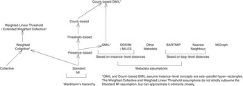
In this section we review the MI assumptions/concept classes that have been proposed, and briefly discuss the algorithms that have been developed to learn models of MI data under these assumptions. The relationships between the various MI assumptions are shown in Figure 2.
Relationships between multi-instance (MI) assumptions. Arrows indicate increasing generality. GMIL, generalized multiple instance learning; DD, diverse density; SVM, support vector machine; MILES, multiple-instance learning via embedded instance selection

3.1 Weidmann’s concept hierarchy for instance-based generalized MI learning
Weidmann et al. (Reference Weidmann, Frank and Pfahringer2003) formulated a hierarchy of generalized instance-based assumptions for MI learning. The hierarchy consists of the standard MI assumption and three types of generalized MI assumptions, each more general than the last.
To illustrate the three types of generalized MI assumptions, we will follow Weidmann (Reference Weidmann2003) and use an extended version of Chevaleyre and Zucker’s (Reference Chevaleyre and Zucker2001) simple jailer problem (discussed earlier in Section 2.3). Recall that in the simple jailer problem, each bag is a keychain containing several keys, and a bag is considered to be useful (i.e. positive) if one or more of its keys can unlock a specific door.
3.1.1 Presence-based MI assumption
In presence-based MI learning, the assumption is that a bag is positive if and only if there exist one or more instances in the bag that belong to a set of required instance-level concepts (i.e. have the required hidden instance-level class labels). This can be visualized as a version of the jailer problem where there are multiple locks on the door. To unlock the door, we need at least one key that can open each type of lock on the door.
Formally, let  be a presence-based MI concept, let
 be the set of required instance-level concepts, and let
 be the function that outputs the count of the number of occurrences of a concept in the bag. Then:

It should be noted that the standard MI assumption is a special case of presence-based MI, where  , that is, there is just one required concept.
3.1.2 Threshold-based MI assumption
The threshold-based MI assumption states that a bag is positive if and only if there are at least a certain number of instances in the bag that belong to each of the required concepts. Each concept can have a different threshold. In terms of the jailer problem, this is similar to the presence-based MI jailer problem except that multiple copies of each type of lock are allowed, and keys are consumed during the unlocking process. If there are n copies of a certain lock, then we need at least n keys of the appropriate type to unlock it. This is reminiscent of the Microsoft puzzle game Chip’s Challenge. Footnote 2
To state the threshold-based assumption formally, let us use the same lexicon as before, and let  be a threshold based MI concept. Then we have:

where  is the lower threshold for concept i.
3.1.3 Count-based MI assumption
Under the count-based MI assumption, there is a maximum and a minimum number of instances from each of the required concepts that must be observed in order for a bag to be positive. Imagine this as the threshold-based jailer problem, except that there is also a stingy jailer who despises wastefulness, and will not allow anybody to open the door if they have too many keys of any particular type.
Formally, let  be a count-based MI concept. Then

where  is a lower threshold for concept i, and
 is an upper threshold for concept i.
3.1.4 The concept hierarchy
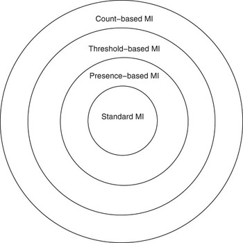
Weidmann et al. (Reference Weidmann, Frank and Pfahringer2003) showed that these assumptions form a hierarchy of generality, where standard MI ⊂ presence-based ⊂ threshold-based ⊂ count-based (see Figure 3 for an illustration).
Weidmann’s hierarchy of instance-based multi-instance (MI) concepts

Therefore, in theory at least, a strong MI learner designed to work under a general assumption should still be able to solve an MI problem where one of the less general assumptions applies. For instance, a strong algorithm designed to use the count-based assumption should work well on a dataset where the generative model is presence-based.
3.1.5 Algorithms and models
The two-level classification (TLC) algorithm (Weidmann et al., Reference Weidmann, Frank and Pfahringer2003) is designed to learn the type of MI concepts that are described in Weidmann’s concept hierarchy, where it is assumed that bag-level class labels are determined by the counts of each instance-level concept in a bag.
TLC learns in a two-step process. The first step learns instance-level concepts using a decision tree. The tree is built on all of the instances in all of the bags in the training data, with class labels of the instances set to the labels of the parent bags. Each node in the tree is considered to represent a candidate concept. Then each bag is converted into a single-instance representation, with an attribute for every node in the tree (i.e. each candidate concept), the value of which is set to the number of instances that reach that node in the decision tree.
The second step learns bag-level concepts, based on the candidate instance-level concepts discovered in the first step. A single-instance learning algorithm is applied to the transformed data. The same mapping is performed at classification time, and the bag-level predictions are made by the single-instance learner. A further (optional) refinement to the algorithm is to use attribute selection to try to eliminate the attributes that do not contribute to the instance-level classification problem learned by the decision tree.
The constructive clustering ensemble (CCE) method (Zhou & Zhang, Reference Zhou and Zhang2007) also uses a propositionalization method that may be appropriate for some Weidmann type concepts. The algorithm uses a clustering method to cluster the instances in the training bags into d clusters. Bags are mapped into a boolean feature space where each attribute corresponds to a cluster, and the value of an attribute is set to 1 if and only if that bag has an instance in that cluster. A single-instance model is built on the resulting dataset. The algorithm is repeated for multiple values of d, and classification predictions are made via a majority vote of the resulting ensemble of single-instance classifiers.
Given that the feature space constructed by CCE represents the presence or absence of instances with certain properties, it appears that this algorithm may be best suited for learning presence-based MI concepts. However, the algorithm could be easily extended to learn count-based concepts if the transformed feature space was modified to include the number of occurrences of the instance-level concepts, as in the earlier TLC algorithm. It should also be noted that Zhou and Zhang’s (Reference Zhou and Zhang2007) results indicate that the algorithm is less accurate when learning on presence-based MI data than TLC (with attribute selection enabled).
3.2 The GMIL assumption
Scott et al. (Reference Scott, Zhang and Brown2005)Footnote 3 introduced a new MI assumption based on theoretical results from geometric pattern recognition. We will refer to this assumption as the GMIL assumption. In this model, there is a set of target points C = {c 1, c 2,…, ck}. A bag is positive if and only if it contains instances sufficiently close to at least r points, out of the k target points.
Scott et al. extend this model to also include a set of repulsion points  . In the extended model, a positive bag may only contain instances that are close to at most s of the repulsion points.
The model can be understood with reference to the ranked half-Hausdorff metric using the weighted infinity norm. The Hausdorff metric (see, e.g. Edgar (Reference Edgar1990)) provides a measure of distance between two bags of points, and is commonly used in computer vision applications. The sets of target points and repulsion points can be viewed as ‘ideal bags’, where positive bags are within a ranked half-Hausdorff distance of some threshold γ from the ideal positive bag, and at least a ranked half-Hausdorff distance of γ′ away from the ideal negative bag.
The Hausdorff distance between bags P and Q is defined to be the largest distance from either a point in P to its closest point in Q, or from a point in Q to its closest point in P, whichever is larger, under some norm. However, this is not robust against noise, so the ranked Hausdorff metric is used: instead of using the largest distance, the sth largest distance is used. Scott et al. compute the distance from the bag to the model (i.e. the half-Hausdorff metric), but not vice-versa, as it is assumed that the model is accurate and does not contain extraneous points.
Scott et al. used the weighted infinity norm as the instance-level distance measure required to compute the Hausdorff distance. The infinity norm defines the length of a vector as ||x||∞ = max(|x 1|,|x 2|,…,|xn|), the largest absolute value of its components. Thus the set of points with a distance of at most d from a point p under the infinity norm are the points within a hypercube of width 2d and center at point p. The weighted infinity norm allows scaling of the vector components, such as for normalization. The hypercubes from the infinity norm are hyperrectangles or ‘boxes’ when the weighted infinity norm is used.
The ranked half-Hausdorff metric using the weighted infinity norm can be stated formally as
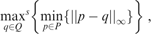
where maxs is the sth max, P is a bag, Q is the set of target points, and ‘−’ denotes standard vector subtraction. Let a bag P be positive if and only if the above equation evaluates to at most γ. Then a target concept is a set of k = |Q| axis-parallel target boxes, and a bag is positive if and only if it contains points within at least r = k − s + 1 of the k target boxes.
To also include a set  of k′ axis-parallel repulsion boxes, we must also check that the following formula evaluates to at least γ′, which is another constant:
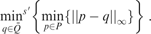
Under this extended model, for a bag to be positive, it must also contain points within at most s′ − 1 of the k′ repulsion boxes.
In terms of Weidmann’s hierarchy, Scott et al.’s MI formulation, without repulsion points, is the same as presence-based MI learning when boxes are viewed as instance-level concepts and the minimum threshold r is equal to the number of target points k. When r ≠ k, Scott et al.’s model is more general than the presence-based MI model. Weidmann’s threshold and count-based MI concepts generalize presence-based MI concepts in a different fashion to Scott et al.’s model, and neither is strictly more general than the other.
Count-based MI concepts can model repulsion points by setting the maximum count for some instance-level concepts to zero. However, count-based and threshold-based concepts cannot model the case where only r out of k concepts must be present for a bag to be positive. The GMIL assumption cannot represent problems where the number of instances belonging to specific concepts must be within a given range (as in threshold and count-based MI), as only concept presence rather than concept counts are included in the model.
3.2.1 Algorithms and models
Scott et al. (Reference Scott, Zhang and Brown2005) proposed the GMIL-1 algorithm to learn GMIL concepts. The algorithm explicitly enumerates all possible axis-parallel boxes. It creates a single-instance feature space with boolean attributes for each box, signifying whether a bag contains an instance within that box. To reduce the dimensionality of this space, boxes that cover the same instances are grouped together, and only one representative box for each group is used. The training bags are mapped into the feature space, and the single-instance algorithm Winnow (Littlestone, Reference Littlestone1987) is trained on the transformed dataset.
The task of enumerating all axis-parallel boxes is exponential in the number of dimensions, which makes GMIL-1 very inefficient. GMIL-2 Tao and Scott (Reference Tao and Scott2004) is an attempt to improve the computational and memory efficiency of the algorithm. The algorithm is roughly the same as GMIL-1, but it selects groups of boxes in a different way. First, GMIL-2 reduces the number of instances to consider by selecting a subset of representative instances,  . Then it constructs groups by considering the boxes represented by the bounding box of each possible subset of
 . A breadth-first search approach is used to attempt to efficiently find the sets of groups that are geometrically valid, that is, all instances within the bounding box of the group are contained within the group.
Although GMIL-2 is far more efficient than GMIL-1, it still suffers from limited scalability (Tao et al., Reference Tao, Scott, Vinodchandran, Osugi and Mueller2004a). In a further attempt to improve the algorithm’s computational complexity, Tao et al. (Reference Tao, Scott, Vinodchandran, Osugi and Mueller2004a) presented a kernel-based reformulation of the GMIL learning problem. The kernel, k ∧, allows a support vector machine to be applied directly to the problem. As the computation of k ∧ belongs to the complexity class P-complete and thus suffers from severe scalability issues that quickly make the problem intractable as the problem size increases, the authors presented a fully polynomial randomized approximation scheme (FRAPS) for it.
3.3 The count-based GMIL assumption
As mentioned earlier, neither the GMIL assumption nor the count-based MI assumption is strictly more general than the other—some MI concepts can be represented by one assumption and not the other, and vice-versa. Tao et al. (Reference Tao, Scott, Vinodchandran and Osugi2004b) proposed an MI assumption that is more general than both of the assumptions, which we will refer to as the count-based GMIL assumption. Under this assumption, a bag is positive if and only if it satisfies at least r of a set of k concepts, and at most s of a set of k′ ‘repulsion’ concepts. A concept ci is satisfied by a bag B if the number of points in the region of instance space associated with ci is between a certain specified minimum value, ti, and a maximum value, zi.
3.3.1 Algorithms and models
Tao et al. proposed an extended version of the k ∧ kernel, called kmin, which allows a support vector machine to solve the MI learning problem under the count-based GMIL assumption. Unlike the k ∧ kernel, the feature space associated with the kmin kernel includes information related to the number of instances within the box that describes the concept concerned.
3.4 The DD-SVM/multiple-instance learning via embedded instance selection assumption
The DD-SVM (Chen & Wang, Reference Chen and Wang2004) algorithm and its successor multiple-instance learning via embedded instance selection (MILES) (Chen et al., Reference Chen, Bi and Wang2006) also use a generalized MI assumption, where bag-level class labels are determined based on the distance from each of a set of target points. Although the authors of DD-SVM and MILES note that their algorithms do not follow the standard MI assumption, they do not explicitly describe their new assumptions independently from the descriptions of the algorithms. This section attempts to isolate the common assumptions between these algorithms and thus describe the types of MI concepts that the algorithms attempt to learn.
The DD-SVM/MILES assumption is related to Scott et al.’s (Reference Scott, Zhang and Brown2005) GMIL assumption, in that distance from a set of target points is used to determine bag labels. However, ‘distance’ is defined differently, and the r-of-k threshold is not used. As in the GMIL assumption, the target points can be related to either positive or negative concepts. The DD-SVM and MILES methods each include a distance-related measure of similarity between a target point and a bag, and it is assumed that bag-level class labels are in some way determined by these similarity values. In DD-SVM, the similarity function is

where Bij are the instances in the bag Bi, x is a target point and w is a weight vector determining the importance of each feature. In MILES, a Gaussian function is used instead:
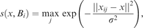
where σ is a scaling factor, which is a parameter to the algorithm. The relationship between the ‘similarities’ to target points and bag-level class labels is dependent on the single-instance base learner that is applied to the data after transformation based on the similarity scores. In the original statement of DD-SVM and MILES, a support vector machine is used. If a linear kernel is used for the SVM, class labels are determined by a weighted linear threshold defined on the similarity values, that is, DD-SVM/MILES concepts are of the form

where T is the set of target points, wk is the weight associated with target point k and b is a bias parameter. If a target point has a positive weight, it can be viewed as being positive—bags with points close to that target point are more likely to be positive; and similarly for negative target points, that is, points with negative weight.
However, alternative single-instance base learners are possible for both DD-SVM and MILES. If we view the algorithms as ‘wrapper’ methods where arbitrary base learners are possible, the assumption is merely that bag-level labels can be determined in some way from the similarities to the set of target points.
3.4.1 Algorithms and models
MILES (Chen et al., Reference Chen, Bi and Wang2006) embeds bags into a single-instance feature space based on similarity scores obtained from Equation 2, and applies the 1-norm support vector machine algorithm to the transformed dataset.
MILES uses the instances in the training bags as candidates for target points. A feature-space mapping is defined, where each attribute represents the closeness of an instance to a candidate target point (i.e. training instance). Each training bag is mapped into this space (with class labels appended), and a single-instance base learner is built on the transformed dataset. At testing time, bags are similarly mapped into the instance-based feature space, and classification predictions are made by the single-instance base learner.
The diverse density support vector machine (DD-SVM) algorithm (Chen & Wang, Reference Chen and Wang2004) is a predecessor to MILES that is conceptually very similar to the later method. Chen et al.’s (Reference Chen, Bi and Wang2006) experimental results show that MILES is much more efficient than DD-SVM in terms of computational complexity, while maintaining similar or better classification accuracy and increased robustness to label noise, hence we do not discuss DD-SVM in detail here.
3.5 The bag-level representation transformation for multi-instance prediction assumption
The BARTMIP algorithm (Zhang & Zhou, Reference Zhang and Zhou2009) is closely related to MILES, and thus implicitly relies on a related MI assumption. While MILES assumes that bag labels are related to the instance-level distances from a set of target points, the BARTMIP method assumes that bag labels are related to distances from target bags.
Distances between bags of points can be computed via the Hausdorff distance (see Section 3.2). Zhang and Zhou use three different variants of the Hausdorff distance to define bag-level distances: the maximal, minimal and average Hausdorff distances.
The (maximal) Hausdorff distance between two sets of points (or bags) A and B is the largest Euclidean distance between a point in A and its closest point in B, or vice versa. Formally, the Hausdorff distance is defined as

where

The minimal Hausdorff distance was proposed by Wang and Zucker (Reference Wang and Zucker2000) in the context of a simple nearest-neighbor MI learning algorithm that is discussed in more detail in Section 3.11. In this variant, the h function is replaced by a function h 1, where

Note that the minimal Hausdorff distance is simply the shortest distance between a point in A and a point in B. It can be stated as

Zhang and Zhou additionally proposed the average Hausdorff distance, which is defined to be the average distance between a point in one bag and its closest point in the other bag:

The choice of distance measure determines the set of MI concepts that can be represented. Clearly, alternative bag-level distance measures could potentially be used if appropriate for a specific problem domain.
3.6 Algorithms and models
The BARTMIP algorithm performs an initial bag-level clustering step on the training bags using the k-medoids algorithm adapted to MI learning by using a Hausdorff distance variant for its distance function. As well as grouping the bags into k clusters, the clustering algorithm also outputs the medoid Footnote 4 of each cluster.
The training bags are then mapped to a k-dimensional single-instance feature space, where the ith attribute corresponds to the distance of the bag to the ith medoid, under the same bag-level distance measure that was used in the clustering step. The class labels of the original bags are appended to the transformed instances, and a single-instance base learner is applied to the resulting feature space. At classification time, the mapping is performed to the test bags and predictions are made by the single-instance base learner. Note that this method is identical to MILES, except for the different feature-space transformation used.
3.7 The collective assumption
Under the standard MI assumption, only a few special instances (those with a ‘positive’ label) can have any influence on the class label. In contrast, the collective assumption is an MI assumption, where all instances in a bag contribute equally to the bag’s label (Xu, Reference Xu2003).
The collective assumption, designed as a general alternative to the standard MI assumption, was not precisely defined by Xu (Reference Xu2003). However, all algorithms in (Xu, Reference Xu2003) that were designed to use this assumption actually depend on the same specific generative model. We will therefore use the term collective assumption to refer to this specific model.
The collective assumption is motivated by a view of the nature of MI bags that is based on probability theory. Under this view, a bag is not a finite collection of fixed elements (as is generally assumed), but instead is a sample of an underlying population specific to that particular bag. Here, a bag can be modeled as a probability distribution Pr(X|b) over the instance space, where the observed instances were generated by random sampling from that distribution.
Instances are assumed to be assigned class labels according to some (typically unknown) probability function (or non-deterministic probabilistic process) g(x) = Pr(Y|x). Under the collective assumption, the bag-level class probability function is determined by the expected class value of the population of that bag. Let c be a class label ∈Y = {0,1}, and let b be a bag. Then

To compute this exactly, we must know Pr(x|b), the probability distribution for the bag. However, this is generally not known in practice so the sample provided by the instances in the bag is used instead:
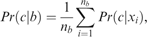
where nb is the number of instances in the bag. In the limit, as the sample size approaches infinity, the sample version of the equation will approach the population version.
3.7.1 Algorithms and models
Xu (Reference Xu2003) developed statistical algorithms for learning this kind of probabilistic concept, the most notable of which are versions of logistic regression and boosting, upgraded to solve MI learning problems under the collective MI assumption (see also (Xu & Frank, Reference Xu and Frank2004)).
Frank and Xu (Reference Frank and Xu2003) also investigated a simple heuristic algorithm called MI Wrapper for applying single-instance learners under the collective assumption. The first step of the MI Wrapper algorithm is to collect all of the instances from all of the bags, and label each of them with the label of the bag that they came from. This effectively creates a propositional (i.e. single-instance) dataset. The algorithm then weights all of the instances so that each bag has equal total weight. A single-instance learner is applied to this propositional dataset. At classification time, the single-instance learner predicts class probabilities for all of the instances in the bag for which the classification is to be predicted. The output is merely the average (arithmetic or geometric) of the predicted instance-level class probabilities. Using the arithmetic mean at prediction time, the method applies the ‘sample’ version of the collective assumption formula when making predictions.
3.8 MI assumptions using instance weights
In the collective assumption, each instance receives equal weight when computing bag-level class probabilities. Foulds (Reference Foulds2008) introduced two MI assumptions based on the notion of instance weights that determine the level of influence that instances have on bag-level class labels. The weighted collective MI assumption is an extended version of the collective assumption that incorporates a weight function over instance space as well as a probability function, while the weighted linear threshold MI assumption is based on linear classification models from single-instance learning. Although the two assumptions are quite different in form, and each facilitates different concept description models and algorithms, it can be shown that the weighted linear threshold assumption is equivalent to an extended version of the weighted collective assumption in terms of the MI concepts that can be represented (Foulds, Reference Foulds2008).
3.8.1 The weighted collective assumption
While under the collective assumption it is assumed that instances contribute equally and independently to bag-level class labels, the weighted collective assumption asserts that each instance contributes independently but not necessarily equally to the class label of the bag. This is achieved by incorporating a weight function into the collective assumption:

where  is a weight function from instance space to the positive real numbers (not including zero) that determines the level of influence that an instance has on the bag-level class label.
The weighted collective assumption, as stated in Equation 3, is a probabilistic model. Sometimes, however, a deterministic classifier may be more appropriate. It is also possible to state a deterministic version of the assumption in the standard fashion, where bags are labeled with the ‘most likely’ class according to the probability function described in Equation 3. In the case of binary classification, this corresponds to:

Here, t is the decision variable, the sign of which determines the classification outcome. This MI assumption is more powerful than the collective assumption because it allows some instances to be ignored when determining bag-level class labels. The collective assumption gives all instances in a bag the same weight, which means that every instance must be taken into account, and irrelevant instances may bias the class probability estimates in some problem domains. For instance, the collective assumption cannot model the standard MI assumption, where only a few (positive) examples affect the class labels of bags. Under the weighted collective assumption, the standard MI assumption can be very closely approximated by giving positive instances a large weight and setting all other weights to values close to zero.
3.8.2 The weighted linear threshold MI assumption
The weighted linear threshold MI assumption is so named because the accumulated (signed) weights for a bag are compared against a threshold to obtain a classification. A weight function  and a classification function cwlt(x) : χ→{+1,−1} are defined over instance space. Instances belonging to the positive class (cwlt (x) = +1) influence their parent bag toward a positive class label, and instances belonging to the negative class (cwlt(x) = −1) influence their bag toward a negative class label. The weight of an instance determines the strength of that instance’s influence on bag-level class labels.
Formally, let  be a weighted linear threshold MI concept. Then νwlt is of the form

Here, b is a bias variable, which determines the location of the decision boundary. This formulation of weight-based MI learning is inspired by linear classification in single instance learning. Recall the classification equation for a linear classifier:

In the weighted linear threshold model, instances are treated analogously to attributes in the case of linear classification. The class cwlt (x) of an instance corresponds to an attribute value mi. Instance weights wwlt (x) in the MI assumption correspond directly to attribute weights wi in a linear classifier. The bias parameter b performs an identical function to the parameter b in the linear classification model.
It can be shown that the weighted linear threshold assumption is at least as powerful as the deterministic version of the weighted collective assumption (in terms of the set of representable concepts). An arbitrary deterministic weighted collective concept can be converted into a weighted linear threshold concept using the following formula (Foulds, Reference Foulds2008):

where

The converse is also true with one restriction: any weighted linear threshold concept where b = 0 can be represented as a deterministic weighted collective concept. This restriction can be eliminated; by introducing a bias parameter bedw into the formulation, the extended deterministic weighted collective assumption becomes equivalent to the weighted linear threshold assumption:

3.8.3 Algorithms and models
Implementing the weighted collective assumption requires a method for learning instance weights. Foulds (Reference Foulds2008) investigated an iterative framework for learning instance weights (IFLIW), a heuristic algorithm for learning weighted collective assumption concepts. The algorithm is an extension of the MI Wrapper approach from Section 3.7.1. IFLIW uses MI Wrapper to learn the class probability function pr(c|x) via the simple propositionalization method described in Section 3.7.1 and a single-instance base learner. The challenge, however, is to estimate the weight function. An iterative method is applied, where instance weights of the training data are updated according to an update function, and the MI Wrapper model is rebuilt using the new weights. The update function that is used is:

where x.weight is the weight of instance x, infogain is the information gain of pr(c|x), the class probability distribution for the instance x predicted by the single-instance base classifier, relative to pr(c), the prior class probabilities computed from the class frequencies in the training data. The iteration continues until a stopping criterion is met. The weight function is then estimated using a regression model built on the training instance weights.
It is also possible to learn a model based on the weighted linear threshold assumption. The MILES method from Section 3.4 can be modified so that it learns weighted linear threshold concepts when a linear classifier is used as the base learner (Foulds, Reference Foulds2008). This is achieved by using an alternative similarity measure between a bag and a target point.
Recall that the similarity measure s(x, B) used in MILES (Equation 2) includes a max operator, which effectively selects only the closest instance in the bag B when determining the similarity value. This is based on Maron’s (1998) most likely cause estimator from the diverse density framework. The models learnt by MILES (with a linear classifier as the base learner) can be understood as being similar to weighted linear threshold concepts, except that the use of the max operator in the similarity measure means that instance weights are bag-dependent, as only the closest instance in the bag to each target point contributes to the bag-level classification. By simply replacing the max operator with a sum operator, the bag-dependence is removed, resulting in a true weight function over instance space. The resulting similarity measure, called yet another radial distance-based similarity measure (YARDS; Foulds, Reference Foulds2008), is defined as follows:
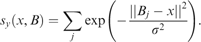
Hence, by replacing the similarity measure s(x, B) in the MILES algorithm with the YARDS similarity measure sy(x, B), MILES can be adapted to learn weighted linear threshold concepts. The YARDS method can represent weighted linear threshold concepts where the weight function is the sum of a set of Gaussian-like influence functions, and makes the further assumption that the peak (or trough) of each of the Gaussian-like functions is at the location of an instance from one of the training bags.
3.9 Metadata-based assumptions
A simple approach to MI learning is to perform propositionalization by replacing each bag with a feature vector consisting of metadata features derived in some way from the instances in that bag. A single-instance learning algorithm can then be applied directly to the transformed version of the dataset. At classification time, new bags are mapped into the metadata feature space, and predictions are made by outputting the prediction of the single-instance learner for the transformed version of the bag. Xu (Reference Xu2003) refers to methods of this kind as metadata approaches.
When this type of method is used, the implicit assumption is merely that the classification labels of the learning examples are directly related to the metadata. We will therefore refer to this type of MI assumption as a metadata assumption.
3.9.1 Algorithms and models
The MILES, YARDS, BARTMIP, TLC and CCE algorithms discussed above all use feature-space transformations, where bags are mapped to single-instance feature vectors, and single-instance algorithms are applied to the resulting datasets. These methods can therefore be viewed as metadata approaches. However, the feature spaces used by these methods are intended to represent more sophisticated MI concepts, and are perhaps better understood with respect to the underlying MI assumptions that the feature-space transformations are designed to encode. In contrast, we will now describe a method that uses simple summary statistics as metadata.
Using this approach, MI learning problems are converted into single-instance problems by replacing each bag with a feature vector consisting of summary statistics derived from the instances in that bag. This method originates from a similar approach to propositionalization for relational data known as relational aggregations (RELAGGS) (Krogel & Wrobel, Reference Krogel and Wrobel2002). We will follow Dong (Reference Dong2006), and refer to the approach based on summary statistics as simple MI.
Dong described three versions of simple MI, each of which differs only in the type of summary statistics used for the single-instance feature space. The first two methods merely average the values of the instances in a bag for each dimension, using either the arithmetic or the geometric mean. Formally, the two methods can be defined as follows: if b is a bag with instances from feature space χ = (x 1, x 2,…, xn), then b is mapped to  , where
 is the arithmetic (or geometric) mean of the instances in the bag.
The third option is called the ‘minimax’ method. Here, the minimum and maximum values of each variable are recorded for each bag. This method is equivalent to Gärtner et al.’s (Reference Gärtner, Flach, Kowalczyk and Smola2002) minimax kernel, used as a kernel in a standard support vector machine algorithm. Using the same notation as before, each bag b is mapped to (min x 1, min x 2,…, min xn, max x 1, max x 2,…, max xn). The new feature space contains 2n dimensions.
The main advantage of simple MI is that it is extremely fast. The computation of the feature-space transformation is trivial, and the single-instance base learner only has to learn from as many instances as there are bags in the training set, regardless of how many instances are contained inside the bags. Of course, this simple model is not able to represent some types of problems. However, Dong found that simple MI (with appropriate base learners) performs surprisingly well on many datasets, even outperforming all of the special-purpose MI algorithms that were investigated in some cases.
A more sophisticated metadata approach is used by the multiple-instance learning using class conditional log likelihood ratio (MICCLLR) algorithm (El-Manzalawy & Honavar, Reference El-Manzalawy and Honavar2007), which performs propositionalization by replacing each bag by a feature vector containing statistics computed based on the class conditional log-likelihood ratios of the attribute values of the instances in the bags. These statistics are computed using the relative frequencies of attribute values and class labels in a flattened version of the MI dataset (using the same method as in the MI Wrapper algorithm from Section 3.7), under the assumption that attribute values are conditionally independent given the class value. As the authors note, Gärtner et al.’s kernel (or equivalently, the minimax simple MI method) may not be able to represent binary data well, unlike MICCLLR; however, the former method does not rely upon the conditional independence assumptions used by the latter.
MI learning algorithms can also be said to rely on a metadata assumption if they are equivalent to a metadata approach for some feature space transformation, even when the algorithm does not explicitly perform the transformation. Learning algorithms of this type include the Relic MI decision tree learner (Ruffo, Reference Ruffo2000) and Gärtner et al.’s (Reference Gärtner, Flach, Kowalczyk and Smola2002) KMI MI kernel method. Relic is an information gain-based decision tree learner that has been upgraded to handle MI data by defining a test-selection criterion for MI bags. Although Relic does actually not perform propositionalization, Xu (Reference Xu2003) showed how, in the case of data with numeric attributes, Relic is equivalent to the minimax version of simple MI with a decision tree base learner, and hence effectively relies upon the same MI assumption.
Gärtner et al. (Reference Gärtner, Flach, Kowalczyk and Smola2002) presented MI kernels that can be used to apply a standard SVM algorithm directly to MI data. As well as the aforementioned minimax kernel, they also proposed the MI kernel KMI, a variant of the set kernel (Gärtner, Reference Gärtner2000). The kernel is defined as
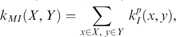
where  is an arbitrary instance-level SVM kernel kI, raised to the pth power. As products of kernels are kernels,
 is also a kernel. Gärtner et al. showed that for a sufficiently large p, any standard MI concept is separable (and thus representable by an SVM using that kernel) assuming that the underlying instance-level concept is separable. It follows from this result that MI concepts that respect the standard MI assumption (with separable instance-level concepts) can be learnt by this method. However, this method does not actually make any use of the standard MI assumption, and can in fact be shown to use a metadata assumption.
Using the fact that the dot product is distributive over scalar multiplication, it is not hard to show that KMI can be rewritten as

where φI (x) is the feature space transformation implicit in the kernel  . Thus, an SVM using the KMI kernel is equivalent to propositionalizing via mapping each bag X to ∑x ∈X φI (X), and applying a standard SVM using a linear kernel to the resulting dataset.
Later, Cheung and Kwok (Reference Cheung and Kwok2006) proposed a regularization framework for MI learning via SVMs using a loss function that encodes a trade-off between Gärtner et al.’s KMI model and an SVM algorithm based on the standard MI assumption that is due to Andrews et al. (Reference Andrews, Tsochantaridis and Hofmann2002). The trade-off is accomplished via a weight parameter λ in the loss function. The implicit assumption of this method is that bag-level class labels are determined by some combination of the KMI metadata assumption and the standard MI assumption.
3.10 The MI graph assumption
Zhou et al. (Reference Zhou, Sun and Li2009) proposed algorithms that depend upon the assumption that the spatial relationships between instances in bags are important contributors to bag labels. Consider the ε-graph of a bag, which has nodes for each instance, and edges exist between nodes if and only if the distance between their associated instances (under some metric) is less than a fixed threshold ε. The edges are weighted according to the affinity of the two nodes—Zhou et al. set the weights to be the normalized reciprocal of the (non-zero) distance between them. The assumption, which we will call the MI graph assumption, is that bag labels are in some way determined by the properties of the ε-graph.
3.10.1 Algorithms and models
The MIGraph and miGraph algorithms (Zhou et al., Reference Zhou, Sun and Li2009) apply support vector machines to MI data by using graph kernels on the ε-graphs of the bags. Although any graph kernel could be used, Zhou et al. define two new kernels based on Gärtner et al.’s MI kernel. The MIGraph and miGraph methods differ only in the kernels used. MIGraph uses the kernel kG, defined as

where E(I) is the edge set of bag I, and knode and kedge are positive semidefinite kernels defined on nodes and edges, respectively. Zhou et al. use the Gaussian radial basis function (RBF) kernel for knode. For the kedge kernel, they define a kernel with the property that edges are similar if their ending nodes have similar degree, taking the edge weights into account. Note that the node portion of the kernel kG is the same as Gärtner et al.’s MI kernel.
As the computational complexity of kG is dominated by the number of edges in X and Y if the graphs are not sparse, it can be computationally expensive to compute the kernel function. To counter this, Zhou et al. introduce the miGraph algorithm, where the kg kernel is used:

where WIi is the reciprocal of the number of instances from bag I in an ε-ball around instance i (including itself). In (Zhou et al., Reference Zhou, Sun and Li2009), the WIis are computed using the Gaussian distance, consistently with the Gaussian RBF kernel used for knode. The authors describe kg as a soft version of a clique-based graph kernel; it behaves identically to a clique-based kernel when all instances are clustered into cliques.
3.11 Nearest neighbor assumptions
In traditional single-instance learning, the k-nearest neighbor algorithm is a simple classification method, where examples are labeled according to the majority class of the k-closest training examples. Here, ‘closest’ is easily defined using a distance metric such as the Euclidean distance.
In MI learning, it is not as immediately obvious how distances between bags should be computed. Wang and Zucker (Reference Wang and Zucker2000) used the maximal and minimal Hausdorff distance for this purpose (see Section 3.5 for more information on this distance). Zhou et al. (Reference Zhou, Sun and Li2009) note that the graph edit distance (Neuhaus & Bunke, Reference Neuhaus and Bunke2007), as computed on the ε-graphs of the bags, could be used as a metric for k-nearest neighbors.
In nearest-neighbor approaches a specific kind of relationship between bags and class labels is not directly assumed. Instead, the implicit assumption is that bags that are ‘similar’ according to the distance measure used are likely to have the same class label. This is closely related to the BARTMIP assumption (Section 3.5). Note that there is no clear relationship between the nearest neighbor assumption (at least when using variants of the Hausdorff distance) and the standard MI assumption.
3.11.1 Algorithms and models
Wang and Zucker proposed two variants of the standard k-nearest neighbor algorithm. In these methods, neighbors are computed in the normal way via the (maximal or minimal) Hausdorff distance; the difference is in the method for selecting the label of an example given a set of neighbors.
These methods were motivated by the authors’ observation that predicting the majority class of the neighbors does not always give the optimal classification result. Their Bayesian-K-nearest neighbor algorithm uses a Bayesian method for predicting the most likely class given a set of neighbors, while the Citation-KNN algorithm is based on the notions of references and citers from the field of library and information science—when making a classification decision, not only are nearest neighbors (references) of an example considered, but also bags that consider the example to be a nearest neighbor (citers).
The experimental results presented by Wang and Zucker indicate that these methods are very competitive with other algorithms on the musk benchmark datasets. However, a comparison with the standard k-NN majority voting method is not provided. It should also be noted that the Bayesian and Citation alternatives to majority voting are not at all dependent on the MI nature of the data, and are hence equally applicable in a single-instance scenario. Finally, Wang and Zucker used parameter values selected on the test data when comparing their methods to other algorithms, so their comparative results may be optimistic.
4 MI learning in other supervised settings
Although the majority of the research on MI learning has been devoted to classification problems, some work has been done on other supervised MI learning scenarios. The most notable of these are MI multi-label learning (Zhou & Zhang, Reference Zhou and Zhang2006) and MI regression (Ray & Page, Reference Ray and Page2001; Amar et al., Reference Amar, Dooly, Goldman and Zhang2001). Similarly to MI classification, any learning approach in these scenarios must depend upon an implicit assumption regarding the nature of the relationship between instances and bag labels; we therefore discuss these assumptions in this section.
Other interesting learning scenarios using MI representations include MI clustering (Zhang & Zhou, Reference Zhang and Zhou2009; Kriegel et al., Reference Kriegel, Pryakhin and Schubert2006), learning instance-level classifiers from bags labeled with a percentage of positive instances (Kück & de Freitas, Reference Kück and de Freitas2005), and predicting the salience of instances in an MI regression setting (Wagstaff & Lane, Reference Wagstaff and Lane2007). None of these scenarios involves bag-level predictions, however, so we do not consider them in this paper.
4.1 MI multi-label learning
In traditional supervised learning, multi-class learning problems contain more than two classification categories, but each learning example belongs to exactly one of these categories. An extension to this is multi-label learning, where the categories are not mutually exclusive, so that each example may belong to several class categories (Schapire & Singer, Reference Schapire and Singer2000).
Zhou and Zhang (Reference Zhou and Zhang2006) formalized MI multi-label learning (MIML), where each MI bag may be associated with multiple class labels. In their formulation, the task in MIML is to learn a function of the form fMIML:2χ→2Y, where χ is the instance space, and Y is the set of class categories. Given that MI examples are really bags (multi-sets) rather than sets, we modify this definition to be  (see Section 2.3.1 for more information on this notation).
As Zhou and Zhang observe, MI learning and multi-label learning are both natural generalizations of traditional single-instance learning, and MIML is a generalization of both of these. In MIML, it is clear that the standard MI assumption is not directly applicable, as that assumption is dependent on the learning task being a binary classification problem. Other assumptions regarding the relationships between the instances and the bag-level labels are required for MIML.
Zhou and Zhang proposed two solution frameworks for applying single-instance learners to solve MIML problems. Although they did not discuss the types of concepts that these frameworks are appropriate for, we will attempt to unify them under a more general algorithm template, and thus expose the MIML assumptions used by both methods.
Before discussing these solution frameworks, it is instructive to first consider a method for converting multi-label problems to single-label problems, used by both of Zhou and Zhang’s MIML approaches. The method is referred to by Tsoumakas and Katakis (Reference Tsoumakas and Katakis2007) as problem transformation method PT4. In this method, the multi-label problem is converted into a set of binary classification problems—one for each of the labels. For each label, a dataset is created where the multi-label training examples that are associated with that label are tagged as positive in the new dataset, and are otherwise tagged as negative. Multi-label predictions are made by building a single-label classifier on each of the new datasets, and outputting the union of the positive predictions made by these classifiers.
The first solution framework proposed by Zhou and Zhang (Solution 1) is to use MI learning as a bridge between MIML and single-instance learning. The MIML problem is converted to a set of MI problems using PT4. Zhou and Zhang were interested specifically in methods that use traditional single-instance algorithms to solve MIML problems, and hence their formulation of Solution 1 insists on the use of an MI method that can be solved using a single-instance algorithm. Thus an MI method that applies a single-instance algorithm, such as MI Boosting (Xu & Frank, Reference Xu and Frank2004), is then applied to the resulting MI problems.
However, it is clear that any arbitrary MI learning algorithm could in fact be applied. We will refer to this relaxed version of the Solution 1 framework as MIML_PT4. Here, the assumption is that the MI concept corresponding to each label can be learned under the assumption used by the MI base learner. For example, when the MI base learner is Xu and Frank’s (Reference Xu and Frank2004) MI boosting algorithm, the implicit assumption is that the concept associated with each of the labels is a collective assumption MI concept. We shall call this general MIML assumption the MIML_PT4 assumption.
Zhou and Zhang’s other solution framework (Solution 2) uses multi-label learning as the bridge between MIML and traditional single-instance learning. First, a propositionalization method is used to map the MI bags into a single-instance feature space, retaining the multiple labels, resulting in a single-instance multi-label dataset. This new learning problem is transformed into a set of traditional single-instance single-label datasets by applying PT4, and hence is solved by building single-instance models on the resulting datasets.
However, if we view the propositionalization step in Solution 2 as the application of a ‘wrapper’-type MI algorithm, Solution 2 can in fact also considered to be within the MIML_PT4 framework. This is because the order of the transformations is not important—the result is the same whether we apply PT4 and then use the wrapper method to propositionalize the data (MIML_PT4), or propositionalize first and then apply PT4 (Solution 2). Hence, the MIML_PT4 assumption applies to Solution 2 algorithms—it is assumed that the MI assumption used by the propositionalization algorithm applies to each of the MI concepts associated with the MIML labels.
4.1.1 Algorithms and models
Zhou and Zhang’s (Reference Zhou and Zhang2006) MimlBoost algorithm uses MI Boosting (Xu & Frank, Reference Xu and Frank2004) as the MI base learner for Solution 1, while their MimlSvm algorithm uses the constructive clustering propositionalization method (Zhou & Zhang, Reference Zhou and Zhang2007) and an SVM base learner to implement Solution 2.
4.2 MI regression
At the International Conference on Machine Learning in 2001, Ray and Page (Reference Ray and Page2001) and Amar et al. (Reference Amar, Dooly, Goldman and Zhang2001)Footnote 5 independently formulated multiple instance regression, where bags are associated with real-valued labels instead of the usual binary class labels. The task is again to predict these labels. Similarly to MI classification, MI regression is motivated by the drug activity prediction problem. The authors of both papers observe that many drug developers prefer predictions of activity levels of drugs, instead of active/inactive classification predictions. Application areas identified by later authors include aerosol optical depth prediction for climate research (Wang et al., Reference Wang, Radosavljevic, Han and Obradovic2008) and crop yield modeling (Wagstaff & Lane, Reference Wagstaff and Lane2007).
Ray and Page assume that the data is generated by a linear model with Gaussian noise on the real-valued labels. Critically, they further assume that for each bag, there is one instance (referred to as the primary instance) that is responsible for the label. Similarly to the standard MI assumption in classification problems, this further assumption is useful for modeling ambiguity, where the instances in a bag represent different views or different states of an object, and it is unknown which of the instances is responsible for the class label. We thus refer to it as the standard MI regression assumption.
Amar et al. proposed the direct application of the Citation-KNN algorithm (Wang & Zucker, Reference Wang and Zucker2000) and traditional k-NN (using the minimal Hausdorff distance) to data with real-valued labels. These methods depend on the same assumption as the nearest neighbor MI classification methods; namely that bags that are similar according to the bag-level distance measure will have similar labels.
The later MI regression algorithms proposed by Wang et al. (Reference Wang, Radosavljevic, Han and Obradovic2008) use the assumption that each bag is generated by some random noise around a point in instance space, which they refer to as a prime instance. Footnote 6 Bag labels are assumed to be generated from the prime instances via some function (with added noise).
Zhang and Zhou Reference Zhang and Zhou(2009) observed that their BARTMIP algorithm (see Section 3.5), which maps bags into a single-instance feature space, can be directly applied to MI regression when a single-instance regression base learner issued—the method works the same way regardless of whether labels are discrete or real-valued. This method could in fact be applied to any other metadata algorithm, such as MILES or simple MI. Under this approach, the metadata assumption used by the corresponding MI classification algorithm is applied in the regression setting.
4.2.1 Algorithms and models
Under Ray and Page’s assumptions, an ideal MI regression model is a hyperplane Y = Xb such that
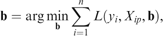
where n is the number of bags, yi is the real-valued label of bag i, Xip is the primary instance of the ith bag, and L is a loss function. Ray and Page use L(yi, Xij, b) = (yi − Xij,b)2, similarly to traditional multiple regression. However, the primary instances Xip are not known at training time, so Ray and Page propose that the ‘best fit’ hyperplane be used instead:

They state that the decision problem for the existence of such a hyperplane can be shown to be NP-complete via a reduction from the 3SAT problem. They therefore instead present an approximation algorithm. Their algorithm is an EM approach, which iteratively improves an initial guess at a hypothesis. In the expectation step, an instance is selected from each bag, namely the one that has the least L-error with respect to the current guess at the hypothesis hyperplane. In the maximization step, ordinary multiple regression is performed to find a hyperplane that best fits the selected instances. These steps are repeated until convergence. As Ray and Page observe, this algorithm can easily be modified to incorporate alternative L-error functions and alternative (possibly non-linear) hypotheses. The algorithm is, however, dependent upon the standard MI regression assumption.
Cheung and Kwok (Reference Cheung and Kwok2006) presented a support vector regression approach for MI regression under the standard MI regression assumption. To make computation feasible, their method relies on the simplifying assumption that the primary instance is the one with the highest output value according to the SVM.
Amar et al. (Reference Amar, Dooly, Goldman and Zhang2001) adapted the diverse density algorithm (see Section 2.4) to MI regression data by using a real-valued version of Maron’s (Reference Maron1998) most likely cause model, and Zhang and Goldman (Reference Zhang and Goldman2001) used a similar method to apply EM-DD (see also Section 2.4) to real-valued data. Here, the assumption is that the closest instance to a certain ‘target point’ is responsible for a bag’s label, which is compatible with the standard MI regression assumption. Bag labels are determined from the distance between the target point and the closest point in the bag by a Gaussian function with a peak at the target point.
Wang et al. (Reference Wang, Radosavljevic, Han and Obradovic2008) proposed MI regression algorithms that are similar to the simple MI and MI Wrapper algorithms described in Sections 3.9 and 3.7, respectively. The Global Pruning-multiple instance regression (MIR) and Balanced Pruning-MIR algorithms are expectation-maximization versions of an MI Wrapper-like approach that discards those instances that are most likely to be noisy in each iteration. It should be noted that these methods are very similar to the IFLIW algorithm from Section 3.8.3, except that sampling is used instead of weighting in the former methods, in order to remove the effects of noisy or unimportant instances.
5 Conclusions
The MI representation is more expressive than the traditional feature-vector model, and is a natural way to describe learning examples in a diverse array of real-world scenarios. Learning from sets of MI examples is a difficult problem because there are many ways that instances can interact with bag-level class labels, and consequently the hypothesis space is very large. This difficulty can (and must) be mitigated by assuming that MI concepts are of some specific form.
The standard MI assumption, namely that bags have a positive class label if and only if at least one instance in the bag is positive, is widely believed to be applicable to drug activity prediction problems such as identifying molecules that emit a musky odor. While this assumption is also a good heuristic for some other problem domains, this does not imply that it will always hold, thus alternative assumptions can be required.
We have reviewed MI assumptions from the literature that have been used for the supervised learning scenarios of classification, regression and multi-label learning with MI data. We have discussed alternatives to the standard MI assumption that have been explicitly introduced by the authors, and also attempted to clarify MI assumptions implicitly used by algorithms where authors do not state them explicitly. We have found that some of the most popular and widely cited MI approaches actually disregard the standard MI assumption. This indicates that this assumption may not be as crucial for the musk problem as was initially hypothesized by Dietterich et al. (Reference Dietterich, Lathrop and Lozano-Pérez1997)—several approaches that depart from the standard MI assumption have been shown empirically to be very competitive on the musk data.
The expressivity of the MI representation is a strong motivation for continued work in this area. As MI learning continues to be applied to a wider selection of practical machine learning problems, the use of appropriate MI assumptions for the problems at hand becomes increasingly important. We therefore anticipate that future research into algorithms and assumptions for the relaxed MI learning problem will prove fruitful.
We do, however, believe that it is important to explicitly state assumptions used by an algorithm whenever the standard MI assumption is not used. Researchers and practitioners need to be aware that different MI problem domains may require different MI assumptions, and the standard MI assumption is not always applicable. It is important to verify that the MI assumption used by an algorithm is at least plausible for the problem at hand.
A task that is of particular interest is to find more effective and generally applicable algorithms for learning visual concepts, such as for image classification and content-based image retrieval. The MI representation allows for concept descriptions that are defined upon the interaction of instance-level concepts, which is a very natural way to describe visual concepts. Different visual concepts are likely to require vastly different interactions between instances and bag-level class labels—for example, the banana concept is likely to be very different to the beach concept—so there is significant scope for work on alternative MI assumptions in this domain.