1 Introduction
The mechanism of flapping-wing aerodynamics provides an efficient way to generate necessary lift and thrust and is the most common way of flying adopted by birds and insects. In comparison to other flying mechanisms used by nature’s flyers and artificial flying machines, flapping shows many attractive characteristics such as agility, hovering capability, efficiency at low Reynolds number, etc. Although some understanding is achievable through carefully designed numerical simulations (Dong, Mittal & Najjar Reference Dong, Mittal and Najjar2006; Dong & Liang Reference Dong and Liang2010; Liang, Dong & Wei Reference Liang, Dong and Wei2010; Yang, Wei & Zhao Reference Yang, Wei and Zhao2010; Yin & Luo Reference Yin and Luo2010), the problem’s large parametric space prevents further physical understanding and optimization through a direct parametric study.
To achieve an understanding of all the control parameters, one often chooses to reduce the complexity of the physical model and/or the size of parametric space. Based on a quasi-steady model with 11 control parameters, Berman & Wang (Reference Berman and Wang2007) were able to use a hybrid algorithm of the genetic method and simplex method to minimize the power consumption of insect flights. Ghommem et al. (Reference Ghommem, Hajj, Mook, Stanford, Beran, Snyder and Watson2012) used an unsteady vortex-lattice method and a deterministic global optimization algorithm for the optimization of flapping wings in forward flight with active morphing, where only 4–8 parameters were considered. Milano & Gharib (Reference Milano and Gharib2005) applied a genetic algorithm in an experimental setting to maximize the average lift from a flapping flat plate by limiting the number of control parameters to only 4. Trizila et al. (Reference Trizila, Kang, Aono, Shyy and Visbal2011) has used a combined approach with numerical simulation and surrogate modelling to explore a three-parameter design space for a three-dimensional plate in hovering motion. Building a map of the entire desire space is useful for some problems but may not be necessary for others. On the other hand, the computational cost was still high even with a surrogate model and prevents the study from including more parameters, and the accuracy was limited by the surrogate model. There have also been efforts to use gradient-based methods for optimization. Tuncer & Kaya (Reference Tuncer and Kaya2005) and Culbreth, Allaneau & Jameson (Reference Culbreth, Allaneau and Jameson2011) used an gradient-based method to optimize the flapping-wing motion for better thrust and efficiency. They used direct numerical simulation for each set of control parameters and then computed the gradient of the cost function subject to the perturbation of parameters directly by finite difference. Since all parameters were evaluated individually and required their own simulation, the process became extremely expensive, and the former work was limited to 4 parameters and the latter included cases of from 1 to 11 parameters.
Different from the above works, an adjoint-based method is capable of obtaining the gradient information simultaneously for an arbitrary number of input parameters by one single computation in the adjoint space. Consequently, the total computational cost to obtain the sensitivity of a cost function to all control parameters is independent of the number of control parameters. Thus an adjoint-based method is suitable for the sensitivity analysis and optimization of problems with a large input space but a small output space, such as the study of kinematics and deformation of flexible flapping wings. Depending on the order of applying the discretization and adjoint formulation, there are two types of adjoint approaches: the continuous approach (Bewley, Moin & Temam Reference Bewley, Moin and Temam2001; Wei & Freund Reference Wei and Freund2006) and the discrete approach (Lee, Padulo & Liou Reference Lee, Padulo and Liou2011; Jones & Yamaleev Reference Jones and Yamaleev2013). Nadarajah & Jameson (Reference Nadarajah and Jameson2000) and Collis et al. (Reference Collis, Ghayour, Heinkenschloss, Ulbrich and Ulbrich2001) have discussed the pros and cons of the two approaches. In the current work, we take the continuous approach for its simplicity and clarity in the governing equation for adjoint space, which has mathematical terms which may be interpreted as representing the generation, convection and dissipation of adjoint variables (Wang & Gao Reference Wang and Gao2013). However, use of the continuous adjoint approach on flapping wings has been scarce because of the difficulty in defining the perturbation at a moving or deforming boundary (Moubachir & Zolesio Reference Moubachir and Zolesio2006). In their work of applying an adjoint-based method to obtain the gradient information for the shape optimization of a plunging airfoil, Nadarajah & Jameson (Reference Nadarajah and Jameson2007) used a mapping function to transfer the physical domain with a moving boundary to a computational domain with a fixed boundary so that traditional adjoint-based methods for a fixed domain can be directly applied (and the trouble relating to the moving boundary is avoided). Although the idea was straightforward, the mapping function increased considerably the complexity of the formulation even for their simple case where only the shape (as a steady function) of a rigid flapping airfoil was optimized. In other words, Nadarajah and Jameson were only able to optimize the steady part of an unsteady mapping function. When the moving trajectory and dynamics morphing (as an unsteady function) need to be optimized for a flapping wing, the complexity reaches a much higher level and yields the mapping-function approach infeasible. To deal with the increased complexity introduced by an unsteady morphing domain, we choose to apply non-cylindrical calculus (Moubachir & Zolesio Reference Moubachir and Zolesio2006; Protas & Liao Reference Protas and Liao2008) to derive adjoint equations directly in a morphing domain and to optimize the moving boundary in its original space without using a mapping function. The advantage of choosing non-cylindrical calculus over the unsteady mapping function has been demonstrated by Protas & Liao (Reference Protas and Liao2008) with a comparison of the two approaches in deriving the adjoint equation for a one-dimensional heat equation with a moving boundary.
Using a continuous adjoint approach to handle the large parametric space and non-cylindrical calculus to handle the moving boundary, we can study the optimal moving trajectory and arbitrary deformation of a flapping wing. The optimal solutions of different configurations (a two-dimensional rigid flapping plate, a two-dimensional flexible flapping plate, a three-dimensional rigid flapping plate and a three-dimensional flexible flapping plate) for different control goals (thrust performance, propulsive efficiency and lift performance in hovering) provide a unique opportunity to understand the flapping-wing mechanism and the role of flexibility through a detailed comparison of optimal and non-optimal controls, corresponding flow fields and other aerodynamic performance indicators. The rest of the paper is arranged in the following manner. The governing equations for adjoint-based optimization and the basic gradient formulation are derived in § 2. Details of the numerical simulation are given in § 3. Then, in § 4, there are the validations of gradient information and optimal solutions provided by the adjoint approach. Finally, in § 5, the adjoint-based approach is applied to optimize and study different two-dimensional and three-dimensional flapping-wing cases for the understanding of the flow physics behind different kinematics and flexibility for aerodynamic performance. The final conclusions are given in § 6.
2 Governing equations for adjoint optimization
The basic derivation and notation of the continuous adjoint equations are similar to those used by Bewley et al. (Reference Bewley, Moin and Temam2001) and Wei & Freund (Reference Wei and Freund2006), although those works dealt only with problems with a fixed domain. The inclusion of non-cylindrical calculus to formulate the adjoint equations a with morphing domain or moving boundary has been suggested by Moubachir & Zolesio (Reference Moubachir and Zolesio2006) within a mathematical framework only and later by Protas & Liao (Reference Protas and Liao2008) with numerical implementation for simple problems (e.g. the one-dimensional heat equation). We followed the same idea and extended its application to work for the Navier–Stokes equations with preliminary results shown in our earlier works (Xu & Wei Reference Xu and Wei2013, Reference Xu and Wei2014; Xu et al. Reference Xu, Wei, Li and Dong2015), which eventually lead to the current work with a validation and applications for the optimization and understanding of flapping wings.
2.1 Governing equation and cost function
Though the approach is not limited to a particular shape or motion, for the convenience of discussion, we consider a scenario where a plate is plunging and/or pitching with a prescribed velocity
 $\boldsymbol{V}(t)$
. The flow dynamics is described by the incompressible Navier–Stokes equations,
 $$\begin{eqnarray}\left.\begin{array}{@{}c@{}}\mathscr{N}(\boldsymbol{q})=\mathscr{F}\quad \text{in}~{\it\Omega},\\ \boldsymbol{u}=\boldsymbol{V}\quad \text{on}~\mathscr{S},\\ \boldsymbol{u}|_{t=0}=\boldsymbol{u}_{0}\quad \text{in}~{\it\Omega},\end{array}\right\}\end{eqnarray}$$
where
 ${\it\Omega}$
denotes the fluid domain,
 $\mathscr{S}$
denotes the solid boundary, the primary variable
 $\boldsymbol{q}=[p\;\boldsymbol{u}]^{\text{T}}$
for pressure and velocity, the operator
 $$\begin{eqnarray}\mathscr{N}(\boldsymbol{q})=\left[\begin{array}{@{}c@{}}\displaystyle \frac{\partial u_{j}}{\partial x_{j}}\\ \displaystyle \frac{\partial u_{i}}{\partial t}+\frac{\partial u_{j}u_{i}}{\partial x_{j}}-{\it\nu}\frac{\partial ^{2}u_{i}}{\partial x_{j}^{2}}+\frac{\partial p}{\partial x_{i}}\end{array}\right],\quad \mathscr{F}=0,\end{eqnarray}$$
with the Einstein summation convention being implied for repeated indices and
 $\boldsymbol{u}_{0}$
is an arbitrary initial velocity field.
For demonstration purpose, we pick a simple cost function
 $\mathscr{J}$
, which is to minimize the overall difference between the velocity
 $\boldsymbol{u}$
at a downstream region
 ${\it\Omega}_{o}$
and a target velocity
 $\boldsymbol{u}_{{\it\Omega}_{0}}$
in that region for time period
 $(0,T)$
:
 $$\begin{eqnarray}\mathscr{J}=\int _{0}^{T}\int _{{\it\Omega}_{o}}|\boldsymbol{u}-\boldsymbol{u}_{{\it\Omega}_{0}}|^{2}\,\text{d}{\it\Omega}\,\text{d}t.\end{eqnarray}$$
This choice of cost function also provides the convenience of having an obvious optimal solution:
 $\boldsymbol{u}=\boldsymbol{u}_{{\it\Omega}_{0}}$
, which makes an easy validation of the approach. With the cost function
 $\mathscr{J}$
defined, its sensitivity to control
 ${\it\phi}$
is computed by the perturbed function
 $\mathscr{J}^{\prime }$
subjected to an arbitrary perturbation
 ${\it\phi}^{\prime }$
, and it is defined by the Fréchet differential:
 $$\begin{eqnarray}\mathscr{J}^{\prime }\equiv \lim _{{\it\varepsilon}\rightarrow 0}\frac{\mathscr{J}({\it\phi}+{\it\varepsilon}{\it\phi}^{\prime })-\mathscr{J}({\it\phi})}{{\it\varepsilon}}.\end{eqnarray}$$
When optimization is considered, the gradient
 $g({\it\phi})$
is derived from the above sensitivity analysis to update control variables iteratively by
 $$\begin{eqnarray}{\it\phi}^{new}={\it\phi}^{old}-{\it\alpha}g({\it\phi}^{old}),\end{eqnarray}$$
with a step-size parameter
 ${\it\alpha}$
. The cost of optimization is largely affected by its convergence speed for a typical gradient-based method, so the conjugate gradient method and other numerical methods to accelerate the convergence are normally involved.
The gradient of the flow variables comes from the same definition with the perturbation to control:
 $$\begin{eqnarray}\boldsymbol{q}^{\prime }(t,{\it\phi},\boldsymbol{x})\equiv \lim _{{\it\varepsilon}\rightarrow 0}\frac{\boldsymbol{q}(t,{\it\phi}+{\it\varepsilon}{\it\phi}^{\prime },\boldsymbol{x})-\boldsymbol{q}(t,{\it\phi},\boldsymbol{x})}{{\it\varepsilon}}.\end{eqnarray}$$
For problems with moving/morphing boundaries and the control involving boundary changes, this definition proposes ambiguity on those boundaries. To be consistent with the governing equation for fluid flow dynamics, the derivatives, including the one used for the gradient, are naturally defined in an Eulerian framework. However, all the changes happening on the moving boundaries, including kinematics and deformation, are described in a Lagrangian framework. We cannot describe a boundary perturbation in an Eulerian framework since grid points move frequently on or off (inside or outside) the boundary. Essentially, a bridge is needed to connect the derivation in an Eulerian framework (for the fluid equations) to the derivation in a Lagrangian framework (for the boundary perturbation), in order to derive the continuous adjoint equation for the optimization of control parameters involving boundary movement. Although an unsteady mapping function is a straightforward choice, it is not a feasible solution for many problems because of its complexity in derivation and formulation (Protas & Liao Reference Protas and Liao2008). Alternatively, we choose non-cylindrical calculus as a simple and feasible approach providing the same accuracy (Moubachir & Zolesio Reference Moubachir and Zolesio2006; Protas & Liao Reference Protas and Liao2008).
2.2 Non-cylindrical calculus toolbox
To introduce non-cylindrical calculus, we define a flow map
 $\mathscr{T}$
to describe the time evolution of domain
 ${\it\Omega}$
with control
 ${\it\phi}$
:
 $$\begin{eqnarray}\mathscr{T}(t,{\it\tau},{\it\phi}):{\it\Omega}(t,{\it\phi})\rightarrow {\it\Omega}(t+{\it\tau},{\it\phi}),\end{eqnarray}$$
which requires boundary-to-boundary mapping and no topological change is allowed. Then, the velocity of the flow map,
 $\mathbb{V}$
, is defined by taking the derivative with respect to local time variance
 ${\it\tau}$
,
 $$\begin{eqnarray}\mathbb{V}(t,{\it\phi},\boldsymbol{x})=\left.\frac{\partial \mathscr{T}(t,{\it\tau},{\it\phi},\boldsymbol{x})}{\partial {\it\tau}}\right|_{{\it\tau}=0}.\end{eqnarray}$$
It is reasonable to match the flow map velocity with the physical velocity
 $\boldsymbol{V}$
on the solid boundary
 $\mathscr{S}$
:
 $$\begin{eqnarray}\mathbb{V}(t,{\it\phi},\boldsymbol{x})=\boldsymbol{V}(t,{\it\phi},s)\quad \text{on}~\mathscr{S}.\end{eqnarray}$$
Meanwhile, we define a transverse map
 $\tilde{\mathscr{T}}$
which maps the domain with original control
 ${\it\phi}$
to the domain with perturbed control
 $({\it\phi}+{\it\varepsilon}{\it\phi}^{\prime })$
at the same time:
 $$\begin{eqnarray}\tilde{\mathscr{T}}(t,{\it\varepsilon},{\it\phi}):{\it\Omega}(t,{\it\phi})\rightarrow {\it\Omega}(t,{\it\phi}+{\it\varepsilon}{\it\phi}^{\prime }).\end{eqnarray}$$
A transverse map velocity
 $\boldsymbol{Z}$
is defined with respect to
 ${\it\varepsilon}$
:
 $$\begin{eqnarray}\boldsymbol{Z}(t,{\it\phi},\boldsymbol{x})=\left.\frac{\partial \tilde{\mathscr{T}}(t,{\it\varepsilon},{\it\phi},\boldsymbol{x})}{\partial {\it\varepsilon}}\right|_{{\it\varepsilon}=0}.\end{eqnarray}$$
For a general function
 $f$
, we use the notation
 ${\dot{f}}$
for its derivative in a Lagrangian framework, and
 $f^{\prime }$
for its derivative in an Eulerian framework (i.e. the one used for the Navier–Stokes equations). Here,
 ${\dot{f}}$
is called the non-cylindrical material derivative and is defined by
 $$\begin{eqnarray}{\dot{f}}(t,\boldsymbol{x})\equiv \lim _{{\it\varepsilon}\rightarrow 0}\frac{f(t,{\it\phi}+{\it\varepsilon}{\it\phi}^{\prime },\tilde{\mathscr{T}}(t,{\it\varepsilon},{\it\phi},\boldsymbol{x}))-f(t,{\it\phi},\boldsymbol{x})}{{\it\varepsilon}},\end{eqnarray}$$
and
 $f^{\prime }$
is called the non-cylindrical shape derivative and is related to
 ${\dot{f}}$
by
 $$\begin{eqnarray}f^{\prime }={\dot{f}}-\boldsymbol{Z}\boldsymbol{\cdot }\boldsymbol{{\rm\nabla}}f.\end{eqnarray}$$
The non-cylindrical material derivative also defines the relation between the transverse map velocity
 $\boldsymbol{Z}$
and the flow map velocity
 $\mathbb{V}$
by
 $$\begin{eqnarray}\dot{\mathbb{V}}=\frac{\text{d}\boldsymbol{Z}}{\text{d}t}.\end{eqnarray}$$
2.3 Linearized perturbation equation
With the above toolbox, we can easily derive the linearized perturbation equation for the Navier–Stokes equations using the shape derivative:
 $$\begin{eqnarray}\left.\begin{array}{@{}c@{}}\displaystyle \mathscr{N}^{\prime }(\boldsymbol{q})\boldsymbol{q}^{\prime }=\mathscr{F}^{\prime }\quad \text{in}~{\it\Omega},\\ \displaystyle \boldsymbol{u}^{\prime }=\dot{\boldsymbol{V}}-\boldsymbol{Z}\boldsymbol{\cdot }\boldsymbol{{\rm\nabla}}\boldsymbol{u}\quad \text{on}~\mathscr{S},\\ \displaystyle \boldsymbol{u}^{\prime }|_{t=0}=0\quad \text{in}~{\it\Omega},\\ \displaystyle \dot{\boldsymbol{V}}=\frac{\text{d}\boldsymbol{Z}}{\text{d}t}\quad \text{on}~\mathscr{S},\\ \displaystyle \boldsymbol{Z}|_{t=0}=0\quad \text{on}~\mathscr{S},\end{array}\right\}\end{eqnarray}$$
where
 $$\begin{eqnarray}\mathscr{N}^{\prime }(\boldsymbol{q})\boldsymbol{q}^{\prime }=\left[\begin{array}{@{}c@{}}\displaystyle \frac{\partial u_{j}^{\prime }}{\partial x_{j}}\\ \displaystyle \frac{\partial u_{i}^{\prime }}{\partial t}+\frac{\partial u_{j}^{\prime }u_{i}}{\partial x_{j}}+\frac{\partial u_{j}u_{i}^{\prime }}{\partial x_{j}}-{\it\nu}\frac{\partial ^{2}u_{i}^{\prime }}{\partial x_{j}^{2}}+\frac{\partial p^{\prime }}{\partial x_{i}}\end{array}\right],\quad \mathscr{F}^{\prime }=0.\end{eqnarray}$$
2.4 Adjoint equation and gradient calculation
Adjoint variables
 $\boldsymbol{q}^{\ast }=[p^{\ast }\;\boldsymbol{u}^{\ast }]^{\text{T}}$
and
 $\boldsymbol{Z}^{\ast }$
are introduced as Lagrange multipliers to impose the flow equations and the transverse system, so that we obtain the shape derivative of the enhanced cost function,
 $$\begin{eqnarray}\displaystyle \mathscr{J}^{\prime } & = & \displaystyle \int _{0}^{T}\int _{{\it\Omega}_{o}}2(\boldsymbol{u}-\boldsymbol{u}_{{\it\Omega}_{0}})\boldsymbol{\cdot }\boldsymbol{u}^{\prime }\,\text{d}{\it\Omega}\,\text{d}t\nonumber\\ \displaystyle & & \displaystyle +\,\int _{0}^{T}\int _{{\it\Omega}(t)}\boldsymbol{q}^{\ast }\boldsymbol{\cdot }[\mathscr{N}^{\prime }(\boldsymbol{q})\boldsymbol{q}^{\prime }-\mathscr{F}^{\prime }]\,\text{d}{\it\Omega}\,\text{d}t+\int _{0}^{T}\int _{\mathscr{S}}\boldsymbol{Z}^{\ast }\boldsymbol{\cdot }\left(\frac{\text{d}\boldsymbol{Z}}{\text{d}t}-\dot{\boldsymbol{V}}\right)\text{d}s\,\text{d}t.\end{eqnarray}$$
Using integration by parts to group and separate the perturbation terms, we then have
 $$\begin{eqnarray}\mathscr{J}^{\prime }=b-\int _{0}^{T}\int _{{\it\Omega}(t)}\boldsymbol{q}^{\prime }\boldsymbol{\cdot }[\mathscr{N}^{\ast }(\boldsymbol{q})\boldsymbol{q}^{\ast }-\mathscr{F}^{\ast }]\,\text{d}{\it\Omega}\,\text{d}t,\end{eqnarray}$$
where
 $$\begin{eqnarray}\displaystyle \left.\begin{array}{@{}c@{}}\displaystyle \mathscr{N}^{\ast }(\boldsymbol{q})\boldsymbol{q}^{\ast }=\left[\begin{array}{@{}c@{}}\displaystyle \frac{\partial u_{j}^{\ast }}{\partial x_{j}}\\ \displaystyle \frac{\partial u_{i}^{\ast }}{\partial t}+u_{j}\left(\frac{\partial u_{i}^{\ast }}{\partial x_{j}}+\frac{\partial u_{j}^{\ast }}{\partial x_{i}}\right)+{\it\nu}\frac{\partial ^{2}u_{i}^{\ast }}{\partial x_{j}^{2}}+\frac{\partial p^{\ast }}{\partial x_{i}}\end{array}\right],\\ \displaystyle \mathscr{F}^{\ast }=\left[\begin{array}{@{}c@{}}0\\ 2(u_{i}-u_{_{{\it\Omega}_{0}}i}){\it\chi}_{o}({\it\Omega}_{o})\end{array}\right],\end{array}\right\} & & \displaystyle\end{eqnarray}$$
and
 ${\it\chi}_{o}$
is a characteristic function defined by
 $$\begin{eqnarray}{\it\chi}_{o}=\left\{\begin{array}{@{}ll@{}}1\quad & \text{in}~{\it\Omega}_{o}\\ 0\quad & \text{otherwise}.\end{array}\right.\end{eqnarray}$$
The boundary terms from integration by parts are all included in
 $b$
as
 $$\begin{eqnarray}\displaystyle b & = & \displaystyle \left.\int _{{\it\Omega}(t)}(u_{j}^{\ast }u_{j}^{\prime })\,\text{d}{\it\Omega}\right|_{t=0}^{t=T}+b_{\infty }+\int _{0}^{T}\int _{\mathscr{S}}u_{i}^{\ast }{\it\sigma}_{ij}^{\prime }n_{j}\,\text{d}s\,\text{d}t\nonumber\\ \displaystyle & & \displaystyle -\,\int _{0}^{T}\int _{\mathscr{S}}{u^{\prime }}_{i}[{\it\sigma}_{ij}^{\ast }n_{j}+u_{j}^{\ast }u_{j}n_{i}+u_{i}^{\ast }(u_{j}-V_{j})n_{j}]\,\text{d}s\,\text{d}t\nonumber\\ \displaystyle & & \displaystyle +\left.\int _{\mathscr{S}}Z_{i}Z_{i}^{\ast }\,\text{d}s\right|_{t=0}^{t=T}-\int _{0}^{T}\int _{\mathscr{S}}\left(\frac{\text{d}Z_{i}^{\ast }}{\text{d}t}+Z_{i}^{\ast }\text{div}_{\mathscr{S}}\boldsymbol{V}\right)Z_{i}\,\text{d}s\,\text{d}t-\int _{0}^{T}\int _{\mathscr{S}}\dot{V}_{i}Z_{i}^{\ast }\,\text{d}s\,\text{d}t,\nonumber\\ \displaystyle & & \displaystyle\end{eqnarray}$$
where
 $b_{\infty }$
indicates all far-field terms,
 $n_{i}$
marks the normal direction from solid to fluid,
 $$\begin{eqnarray}\left.\begin{array}{@{}c@{}}\displaystyle {\it\sigma}_{ij}=-p{\it\delta}_{ij}+{\it\nu}\left(\frac{\partial u_{i}}{\partial x_{j}}+\frac{\partial u_{j}}{\partial x_{i}}\right),\\ \displaystyle {\it\sigma}_{ij}^{\ast }=p^{\ast }{\it\delta}_{ij}+{\it\nu}\left(\frac{\partial u_{i}^{\ast }}{\partial x_{j}}+\frac{\partial u_{j}^{\ast }}{\partial x_{i}}\right),\end{array}\right\}\end{eqnarray}$$
with
 ${\it\delta}_{ij}$
Kronecker’s delta and the tangential divergence is defined by
 $$\begin{eqnarray}\text{div}_{\mathscr{S}}\boldsymbol{V}=\left.\frac{\partial \tilde{V}_{i}}{\partial x_{i}}\right|_{\mathscr{S}}-\frac{\partial \tilde{V}_{i}}{\partial x_{j}}n_{j}n_{i},\end{eqnarray}$$
where
 $\tilde{\boldsymbol{V}}$
is the smooth extension of
 $\boldsymbol{V}$
from
 $\mathscr{S}$
to its neighbourhood.
We noticed that the above formulation of
 $\mathscr{J}^{\prime }$
can be largely simplified if the following conditions are imposed:
 $$\begin{eqnarray}\left.\begin{array}{@{}c@{}}\mathscr{N}^{\ast }(\boldsymbol{q})\boldsymbol{q}^{\ast }=\mathscr{F}^{\ast }\quad \text{in}~{\it\Omega},\\ \boldsymbol{u}^{\ast }=0\quad \text{on }\mathscr{S}\cup {\it\Gamma}_{\infty },\\ \boldsymbol{u}^{\ast }|_{t=T}=0\quad \text{in}~{\it\Omega},\\ \displaystyle \frac{\text{d}\boldsymbol{Z}^{\ast }}{\text{d}t}+\boldsymbol{Z}^{\ast }\text{div}_{\mathscr{S}}\boldsymbol{V}=(\boldsymbol{{\rm\nabla}}\boldsymbol{u})^{\text{T}}\boldsymbol{\cdot }{\bf\sigma}\boldsymbol{\cdot }\boldsymbol{n}\quad \text{on}~\mathscr{S},\\ \boldsymbol{Z}^{\ast }|_{t=T}=0\quad \text{on}~\mathscr{S},\end{array}\right\}\end{eqnarray}$$
where
 $()^{\text{T}}$
indicates the transpose. Equation (2.24) defines the adjoint equations with a set of desirable boundary and initial conditions, where
 $t=T$
is considered the ‘initial’ time, since the adjoint system typically evolves backwards in time. With the definition of the adjoint system, equation (2.18) is reduced to:
 $$\begin{eqnarray}\mathscr{J}^{\prime }=-\int _{0}^{T}\int _{\mathscr{S}}\dot{V}_{i}({\it\sigma}_{ij}^{\ast }n_{j}+Z_{i}^{\ast })\,\text{d}s\,\text{d}t.\end{eqnarray}$$
When the control is related to the change of boundary location and corresponding velocity, (2.25) provides a way to compute gradient information as a function of adjoint solutions only. For example, when the control is for trajectory optimization of a rigid body with fixed shape, the gradient is
 $$\begin{eqnarray}g_{i}(t)=-\int _{\mathscr{S}}({\it\sigma}_{ij}^{\ast }n_{j}+Z_{i}^{\ast })\,\text{d}s;\end{eqnarray}$$
when the control is for optimization of an object with arbitrary trajectory and deformation (e.g. a flexible flapping wing), the gradient is instead
 $$\begin{eqnarray}g_{i}(s,t)=-({\it\sigma}_{ij}^{\ast }n_{j}+Z_{i}^{\ast }).\end{eqnarray}$$
It is noticed that the first term in the gradient is for the perturbation of the boundary velocity and is the same as the term derived by the traditional approach for a fixed domain (which can still have velocity control on the boundary), and the second term is for the domain variation and is unique for a moving boundary/domain and the current approach.
3 Numerical algorithm
As one of the advantages of taking the continuous adjoint approach, the choice of numerical algorithm to solve the adjoint equations is independent of the choice for the original flow equations. To test the robustness of our boundary treatment, which is critical to the current boundary control, we applied different moving-boundary treatments to compute the forward (physical) flow field and the backward (adjoint) ‘flow’ field. Three moving-boundary treatments are considered: (i) immersed boundary method (Mittal et al. Reference Mittal, Dong, Bozkurttas, Najjar, Vargas and Von Loebbecke2008), (ii) arbitrary Lagrangian–Eulerian method (Hirt, Amsden & Cook Reference Hirt, Amsden and Cook1974) and (iii) for simple rigid cases, a moving reference frame algorithm (Li, Sherwin & Bearman Reference Li, Sherwin and Bearman2002). The numerical simulations using different boundary treatments yield similar results and efficiency. The results coming from different simulation methods serve as mutual validations, and there is also validation against the work of others (Guilmineau & Queutey Reference Guilmineau and Queutey2002). Since the base cases are fairly simple and straightforward, the validation of the flow solver is not included here for clarity. However, the validation of the adjoint approach, especially in terms of the accuracy of the gradient information, is emphasized and presented in the next section.
A staggered Cartesian mesh with local refinement through stretching functions is chosen for the benefit of both computational efficiency and numerical stability. We apply a second-order central difference scheme for spatial discretization, a third-order Runge–Kutta/Crank–Nicolson scheme for time advancement and a typical projection method for incompressible flow conditions (Yang et al.
Reference Yang, Wei and Zhao2010; Xu et al.
Reference Xu, Wei, Yang and Lee2016). The time step is mainly constrained by the Courant stability condition for a third-order Runge–Kutta scheme (i.e. CFL number,
 ${\rm\Delta}t\max (|u_{i}|/{\rm\Delta}x_{i})$
, smaller than
 $\sqrt{3}$
). It is noted that the current algorithm is picked for the direct numerical simulation (DNS) of fluid flow, therefore the typical limitation of low Reynolds number applies. However, the theoretical framework presented here for the adjoint approach is meant to be general at the level of the equations before discretization and is not limited to any particular numerical treatment. With the similarity shown in the form of adjoint equations and flow equations, we apply similar numerical algorithms to solve the adjoint equations backwards in time, which leads to similar computational cost for the adjoint computation.
The gradient can be achieved after both the flow and adjoint equations are solved once. In some cases, when the control space is large and the gradient is not smooth, it may be necessary to apply a Sobolev inner product (Jameson Reference Jameson2003) or Savitzky–Golay smoothing filters (Press et al. Reference Press, Teukolsky, Vetterling and Flannery1996) to smooth out the gradient. Meanwhile, in the main iteration to update the gradient, the Polak–Ribiere variant of the conjugate gradient method is used; within each main iteration, Brent’s method is used to determine the optimal step size along each direction and this process requires a couple of subiterations (Press et al. Reference Press, Teukolsky, Vetterling and Flannery1996). The same algorithm to reach convergence to an optimal solution has been tested and used before in our earlier work (Wei & Freund Reference Wei and Freund2006).
4 Validation of optimal solution and gradient information
To assure the accuracy of the current approach, in this section we first compare the optimal solution given by the adjoint-based algorithm to a known optimal solution, then make a further comparison between the gradient information computed by the adjoint approach and the gradient computed by a ‘brute-force’ finite difference approach.
Here, we consider a rigid plate plunging normally to an incoming flow. Non-dimensionalized by its own length, the plate has non-dimensional length
 $l=1$
and thickness
 $h=0.04$
, with the initial location
 $-0.5<x<0.5$
and
 $-0.02<y<0.02$
in a computational domain
 $-10<x<10$
and
 $-10<y<-10$
. A
 $300\times 200$
grid is uniformly distributed in the vicinity of the solid plate and then stretched to the far field. The Reynolds number defined by the incoming flow velocity and plate length is
 $Re=100$
. The control
 ${\it\phi}$
is the plunging velocity at each individual time moment, so the velocity along
 $x$
and
 $y$
are respectively:
 $$\begin{eqnarray}\left.\begin{array}{@{}c@{}}V_{1}(t)=0,\\ V_{2}(t)=\{{\it\phi}(t_{1}),{\it\phi}(t_{2}),\ldots ,{\it\phi}(t_{n})\}.\end{array}\right\}\end{eqnarray}$$
The same cost function is used as in (2.3), with an observation region
 ${\it\Omega}_{o}$
(
 $1.4<x<1.6$
and
 $-0.2<y<0.2$
) behind the plate (figure 1).
A typical snapshot showing the plunging plate, the flow (by vorticity contours) and the observation region
 ${\it\Omega}_{o}$
: the solid lines indicate anticlockwise vorticity and the dashed lines indicate clockwise vorticity. (The same notation for vorticity applies to other similar figures in this paper.)

For validation, we first perform a simulation while using the target control
 ${\it\phi}^{(0)}$
, and record the velocity field
 $\boldsymbol{u}_{0}$
in
 ${\it\Omega}_{o}$
as the target velocity. With some arbitrary initial control
 ${\it\phi}^{(1)}$
(different from
 ${\it\phi}^{(0)}$
), the velocity in
 ${\it\Omega}_{o}$
is
 $\boldsymbol{u}$
. The difference between
 $\boldsymbol{u}$
and
 $\boldsymbol{u}_{0}$
, as indicated by the cost function (2.3), should drive the control to match
 ${\it\phi}^{(0)}$
if the optimization algorithm works. Here, the target and initial controls are respectively:
 $$\begin{eqnarray}\left.\begin{array}{@{}c@{}}{\it\phi}^{(0)}(t)=2A_{0}{\rm\pi}k\sin (2{\rm\pi}kt),\\ {\it\phi}^{(1)}(t)=2A_{1}{\rm\pi}k\sin (2{\rm\pi}kt),\end{array}\right\}\end{eqnarray}$$
where
 $A_{0}=0.1$
,
 $A_{1}=0.2$
and
 $k=0.2$
.
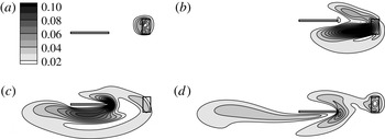
The adjoint field with contours showing the amplitude of the adjoint variable
 $\boldsymbol{u}^{\ast }$
at non-dimensional times: (a)
 $t=9.75$
, (b)
 $t=9$
, (c)
 $t=8.125$
and (d)
 $t=7.375$
. The observation region
 ${\it\Omega}_{o}$
(fixed) and the plate location (moving) are marked for reference.

Usually, there are three types of terms to generate adjoint information (Wang & Gao Reference Wang and Gao2013): the adjoint boundary condition, the production term
 $u_{j}(\partial u_{j}^{\ast }/\partial x_{i})$
and the right-hand side source term
 $\mathscr{F}^{\ast }$
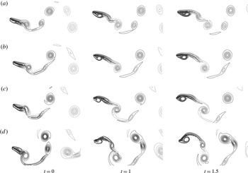
. In the current case, since a homogeneous boundary condition is used, only the other two terms are involved in the generation of adjoint information. Figure 2 shows the snapshots (backwards in time) of the adjoint field, where the adjoint information is marked by the contours showing the amplitude of the adjoint variable
 $\boldsymbol{u}^{\ast }$
. The adjoint information starts from the source term
 $\mathscr{F}^{\ast }$
(currently with the support only in
 ${\it\Omega}_{o}$
). Then, the adjoint information is strengthened by the production term
 $u_{j}(\partial u_{j}^{\ast }/\partial x_{i})$
, as it is travelling upstream (backwards in time). Once the adjoint information passes the plate and reaches the upstream area with uniform flow, the production term is reduced, and the dissipation term in the adjoint equation takes the dominant role and gradually damps out the adjoint information. During the entire process, the adjoint information is continuously being ‘collected’ at the plate boundary to provide the gradient information for the update of the control
 ${\it\phi}$
. It is worth noting that, although the initial and target controls are given as sinusoidal functions, the plunging velocity has no prior knowledge nor constraint on its function type and the optimal velocity is free to be any arbitrary function in time.
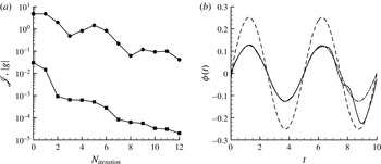
Adjoint-based optimization for the plunging velocity
 ${\it\phi}(t)$
of a rigid plate with the initial control
 ${\it\phi}^{(1)}$
: (a) change of the cost function
 $\mathscr{J}$
(▪) and the gradient norm
 $|g|$
(●) with the number of iterations; (b) comparison of the initial control
 ${\it\phi}^{(1)}$
(– – – –), the target control
 ${\it\phi}^{(0)}$
(– ⋅ – ⋅ –) and the optimal control
 ${\it\phi}^{(p)}$
(——).

Figure 3 shows the performance of the optimization algorithm by: (i) checking the change of the cost function and the gradient norm (to show the local slope of the control space) with the number of iterations; (ii) a direct comparison of the control functions (the initial
 ${\it\phi}^{(1)}$
, the target
 ${\it\phi}^{(0)}$
and the optimal
 ${\it\phi}^{(p)}$
). The cost function value is reduced by an order in only 2 main iterations (with several line-minimization steps for each main iteration) and by an order of
 $10^{3}$
in 12 main iterations; the local gradient norm is also reduced by an order of
 $10^{2}$
and reaches a ‘flat spot’ in 12 main iterations. At the same time, the control is changed from the initial
 ${\it\phi}^{(1)}$
to the optimal
 ${\it\phi}^{(p)}$
. As we can expect from the reduction of the cost function, the optimal control matches very well with the target control until approximately
 $t=8$
. The control cannot be improved much after
 $t=8$
because of the information delay due to the distance between the observation region
 ${\it\Omega}_{o}$
, where the cost function is defined, and the plate, where the control is applied. The travelling time between these two points would require the simulation and the cost function to include future events at
 $t>10$
in
 ${\it\Omega}_{o}$
for optimization of the plate velocity in the time period
 $8<t<10$
.
To further confirm the accuracy of the gradient (and the associated efficiency for the optimization), we validate the gradient information itself by a comparison between the gradient obtained by the adjoint approach and the gradient computed directly by a finite difference approach. The finite difference approach perturbs the control with a small value at each time moment individually and calculates the gradient
 $g$
directly from (2.4). Although the direct approach is straightforward and considered accurate, its computational cost is proportional to the number of control parameters. For instance, in the current case of an arbitrary velocity function, we discretized the velocity function to 2000 time moments and the velocity is allowed to have any value for each time moment, thus a forward finite difference approach needs 2001 numerical simulations to have the one-time gradient for the velocity function in time; on the other hand, only 1 adjoint simulation is needed to achieve the same information.
The gradient
 $g$
(○),
 $g_{v}$
(▿),
 $g_{s}$
(▵) and
 $g_{v}+g_{s}$
(
 $+$
) calculated from the finite difference approach. The control for the plunging plate is
 ${\it\phi}^{(1)}(t)$
.

We noticed that the change of the current control at an arbitrary time
 $t_{l}$
(i.e. plate velocity
 ${\it\phi}(t_{l})$
) comes in two different types: (i) the change of boundary velocity (without the change of original moving trajectory),
 $$\begin{eqnarray}{\it\delta}V_{i}(t)=\left\{\begin{array}{@{}ll@{}}{\it\delta}{\it\phi}(t_{l}),\quad & i=2~\text{and}~t=t_{l}\\ 0\quad & \text{otherwise},\end{array}\right.\end{eqnarray}$$
and (ii) the change of boundary trajectory (without the change of original boundary velocity),
 $$\begin{eqnarray}{\it\delta}S_{i}(t)=\left\{\begin{array}{@{}ll@{}}{\it\delta}{\it\phi}(t_{l}){\rm\Delta}t,\quad & i=2~\text{and}~t>t_{l}\\ 0\quad & \text{otherwise},\end{array}\right.\end{eqnarray}$$
where only the second change is associated with a moving-boundary control as well as non-cylindrical calculus. For better understanding, we therefore decouple the two mechanisms and consider them separately. First, we perturb the velocity of the solid boundary without changing its original trajectory and use (2.4) to calculate the gradient due to the boundary velocity perturbation,
 $g_{v}$
; then, we perturb the boundary location without changing its velocity (by adding an opposite velocity at the boundary) and calculate the gradient due to the boundary location perturbation
 $g_{s}$
. Figure 4 shows that the current perturbation is small enough to assume linearity and the superposition of
 $g_{v}$
and
 $g_{s}$
indeed gives the original gradient
 $g$
by perturbing the plate velocity directly.
Comparison of different components and the total gradient
 $g$
between the values computed by the adjoint method (——) and the finite difference approach through direct perturbation (▪): (a) total gradient
 $g$
; (b) component
 $g_{v}$
; (c) component
 $g_{s}$
.

In the adjoint computation, the total gradient can also be separated to one due to the boundary velocity perturbation,
 $$\begin{eqnarray}g_{v}(t)=-\int _{\mathscr{S}}{\it\sigma}_{2j}^{\ast }n_{j}\,\text{d}s,\end{eqnarray}$$
and the other due to the boundary location perturbation,
 $$\begin{eqnarray}g_{s}(t)=-\int _{\mathscr{S}}Z_{2}^{\ast }\,\text{d}s.\end{eqnarray}$$
Figure 5 then compares the gradients computed by the adjoint method with the ones computed by the finite difference method. With a perfect match in
 $g_{v}$
and some small difference in
 $g_{s}$
, the total gradient
 $g$
computed by the adjoint-based algorithm using non-cylindrical calculus shows good accuracy with extraordinary time saving. It is worth noting that, in numerical simulation, the accuracy of the gradient by the adjoint-based algorithm relies heavily on the accurate computation of the derivatives of both flow and adjoint variables at the corresponding solid boundary.
To test the sensitivity of the algorithm to initial values and verify its independence of a particular function format, we run the same test with the same target control
 ${\it\phi}^{(0)}$
but with a very different initial control
 ${\it\phi}^{(1)}$
:
 $$\begin{eqnarray}\left.\begin{array}{@{}c@{}}{\it\phi}^{(0)}(t)=2A_{0}{\rm\pi}k\sin (2{\rm\pi}kt),\\ \displaystyle {\it\phi}^{(1)}(t)=\frac{t}{10}\left(1-\frac{t}{10}\right),\end{array}\right\}\end{eqnarray}$$
with the same
 $A_{0}=0.1$
and
 $k=0.2$
. As it is shown in figure 6, the same convergence rate is observed, and the same optimal solution is reached (for the controllable time region).
Adjoint-based optimization for the plunging velocity
 ${\it\phi}(t)$
of a rigid plate with a different initial control function
 ${\it\phi}^{(1)}(t)$
: (a) change of the cost function
 $\mathscr{J}$
(▪) and the gradient norm
 $|g|$
(●) by the number of iterations; (b) comparison of the initial control
 ${\it\phi}^{(1)}$
(– – – –), the target control
 ${\it\phi}^{(0)}$
(– ⋅ – ⋅ –) and the optimal control
 ${\it\phi}^{(p)}$
(——).

5 Applications and discussion
In this section, the adjoint-based algorithm is applied to three cases: (i) a rigid plate in combined plunging and pitching motion with an incoming flow; (ii) a flexible plate in plunging, pitching and prescribed deformation with an incoming flow; (iii) a three-dimensional (rigid or flexible) plate in hovering motion. For the first two cases, the control goals are drag reduction (i.e. thrust enhancement) and propulsive efficiency improvement; the control parameters include the phase delay between the plunging and pitching (for the rigid plate) and the phase delay and amplitude of the pitching motion and the first two eigenmodes (for the flexible plate). For the last case, the control goal is lift increase; the control parameters include the translational amplitude, the amplitude and phase delay of the rotational motion and (for the flexible plate) the amplitude and phase delay of the first eigenmode in chordwise bending.
The optimal control parameters provide a unique opportunity for the understanding of aerodynamics and its control mechanism through a comparison between the flow under optimal setting and the flow under initial (non-optimal) setting. A detailed analysis is given after each optimization.
The sketch of a rigid plate with a pitching and plunging motion and an incoming flow coming from left to right.

5.1 Optimization of a flapping rigid plate
Our new adjoint approach is first applied to the aerodynamic optimization of a flapping rigid plate. As shown in figure 7, with a horizontal incoming flow, a rigid plate plunges vertically with a periodic motion and pitches at the same frequency about a point at one-third chord length from the leading edge. The plate is the same as the one used in the benchmark case earlier with non-dimensional scale
 $l=1$
and
 $h=0.04$
. The motion trajectory is defined by:
 $$\begin{eqnarray}\left.\begin{array}{@{}c@{}}y(t)=y_{0}\sin (2{\rm\pi}kt),\\ {\it\theta}(t)={\it\theta}_{0}\sin [2{\rm\pi}kt+{\it\varphi}(t)],\end{array}\right\}\end{eqnarray}$$
where
 $k=0.2$
,
 $y_{0}=0.75$
and
 ${\it\theta}_{0}=27.2^{\circ }$
, yielding a Strouhal number of 0.3. The Reynolds number, defined by the plate length
 $l$
and the incoming flow speed
 $U$
, is 300. The case is similar to the one used by Anderson et al. (Reference Anderson, Streitlien, Barrett and Triantafyllou1998), who suggested the critical role of the phase delay between the pitching and the plunging motion in thrust production and propulsive efficiency. Therefore, the phase delay
 ${\it\varphi}(t)$
is chosen to be the control parameter
 ${\it\phi}(t)$
here, and its optimal time dependence is sought by the adjoint approach for drag reduction and better propulsive efficiency.
5.1.1 Optimization for drag reduction
To reduce the drag, we define the cost function accordingly as:
 $$\begin{eqnarray}\mathscr{J}=\frac{1}{TD_{0}}\int _{0}^{T}\int _{\mathscr{S}}{\it\sigma}_{1j}n_{j}\,\text{d}s\,\text{d}t,\end{eqnarray}$$
where
 $D_{0}=1/2{\it\rho}U^{2}l$
. Following a derivation similar to the one shown in § 2.4 and with more details in appendix A, we obtain the perturbed cost function,
 $$\begin{eqnarray}\mathscr{J}^{\prime }=\frac{1}{TD_{0}}\int _{0}^{T}\int _{\mathscr{S}}\left({\it\sigma}_{1j}^{\prime }n_{j}+\frac{\partial {\it\sigma}_{1j}}{\partial x_{j}}Z_{k}n_{k}\right)\text{d}s\,\text{d}t.\end{eqnarray}$$
Choosing the source term and boundary conditions of the adjoint equations to be:
 $$\begin{eqnarray}\left.\begin{array}{@{}c@{}}\mathscr{F}^{\ast }=0\quad \text{in}~{\it\Omega},\\ u_{i}^{\ast }=-{\it\delta}_{1i}\quad \text{on}~\mathscr{S},\end{array}\right\}\end{eqnarray}$$
and obtaining the adjoint equations for
 $Z^{\ast }$
as,
 $$\begin{eqnarray}Z_{i}^{\ast }=-({\it\sigma}_{ij}^{\ast }n_{j}+u_{j}^{\ast }u_{j}n_{i})\quad \text{on}~\mathscr{S},\end{eqnarray}$$
we have the gradient:
 $$\begin{eqnarray}g(t)=\frac{1}{TD_{0}}\int _{\mathscr{S}}Z_{k}\left(-\frac{\text{d}Z_{k}^{\ast }}{\text{d}t}-Z_{k}^{\ast }\text{div}_{\mathscr{ S}}V-Z_{i}^{\ast }\frac{\partial u_{i}}{\partial x_{k}}+\frac{\partial {\it\sigma}_{1j}}{\partial x_{j}}n_{k}\right)\text{d}s.\end{eqnarray}$$
The phase delay is optimized in two steps. First, we consider the phase delay to be a constant in time and search for its optimal value. Second, after the optimal constant is found, we use this value as an initial condition to optimize the phase delay further by allowing its variation in time. The two-step strategy brings the control to a good neighbourhood in a simple control space (with a constant phase delay) before it becomes a more complex control space (with a time-varying phase delay). Thus, the process makes a more efficient and robust algorithm for optimization. The first step, by considering a constant phase delay only, also provides an easier and more practical solution with its single control parameter, and gives an opportunity to understand the mechanism where the dynamics is simple.
In this case, periodic motion is assumed, and the transition stage is removed from both the forward flow and the adjoint flow.
Step 1. Optimization with a constant phase delay
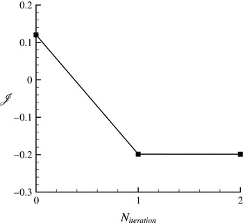
The variation of the cost function for drag reduction with the number of iterations.

The vortex structures of a flapping plate with an initial phase delay
 ${\it\phi}=-30^{\circ }$
during (a) an upstroke and (b) a downstroke.

The vortex structures of a flapping plate with the optimal phase delay
 ${\it\phi}=-77.3^{\circ }$
for drag reduction during (a) an upstroke and (b) a downstroke.

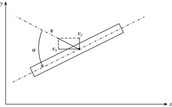
A sketch of the coordinate systems, velocities and angle of attack in a pitching and plunging plate: the velocity of the centre of mass
 $\boldsymbol{v}$
is defined as the relative velocity of the plate with respect to the incoming flow; the angle of attack is denoted by
 ${\it\alpha}$
and is negative in the example shown.

For the constant phase delay, we start with an arbitrary initial value:
 ${\it\phi}=-30^{\circ }$
. It only takes 2 iterations to reach the optimal value:
 ${\it\phi}=-77.3^{\circ }$
. The corresponding drag coefficients, used as the cost function, is reduced from 0.120 to
 $-0.199$
(figure 8). Figures 9 and 10 compare the details in the flow fields with the initial and optimal controls: with the initial control, a strong leading-edge vortex appears at the backside of the plate, which forms a low-pressure region and causes large drag; with the optimal control, there is no obvious leading-edge vortex and the wake shows clearly a thrust-producing
 $2P$
pattern (Williamson & Roshko Reference Williamson and Roshko1988).
To better interpret the result, a quasi-steady model (Pesavento & Wang Reference Pesavento and Wang2004; Andersen, Pesavento & Wang Reference Andersen, Pesavento and Wang2005; Berman & Wang Reference Berman and Wang2007) is adopted to approximate and analyse the associated force
 $\boldsymbol{F}$
on the rigid pitching and plunging plate. We should clearly point out that the quasi-steady model is an approximated solution with fairly aggressive simplification and, on the other hand, the current simulation for the flow and its adjoint system is based on the aforementioned governing equations without such simplification. However, the simplified physics described in the model is derived directly from the original flow equation (with approximation) and helps to understand the flow physics in the analysis later for the optimal solutions from the adjoint-based algorithm. The total force given by the surrounding fluid flow consists of three components: the added mass component
 $\boldsymbol{F}^{\boldsymbol{m}}$
, the lift-induced component
 $\boldsymbol{F}^{\boldsymbol{c}}$
and the viscous drag component
 $\boldsymbol{F}^{{\bf\nu}}$
, which includes both skin friction drag and pressure drag induced by viscosity,
 $$\begin{eqnarray}\boldsymbol{F}=\boldsymbol{F}^{\boldsymbol{m}}+\boldsymbol{F}^{\boldsymbol{c}}+\boldsymbol{F}^{{\bf\nu}}.\end{eqnarray}$$
The added mass term has an almost negligible contribution to the current study, therefore, for clarity, we focus the discussion on the other two force terms. The lift force is normal to the plate’s moving direction and proportional to its velocity and circulation,
 $$\begin{eqnarray}\left.\begin{array}{@{}c@{}}F_{x}^{c}=-{\it\rho}_{f}{\it\Gamma}v_{y},\\ F_{y}^{c}={\it\rho}_{f}{\it\Gamma}v_{x},\end{array}\right\}\end{eqnarray}$$
where the circulation
 ${\it\Gamma}$
depends on the translational speed, the angular velocity
 $\dot{{\it\theta}}$
and the angle of attack
 ${\it\alpha}$
(figure 11):
 $$\begin{eqnarray}{\it\Gamma}=-{\textstyle \frac{1}{2}}C_{T}l\sqrt{v_{x}^{2}+v_{y}^{2}}\sin 2{\it\alpha}+{\textstyle \frac{1}{2}}C_{R}l^{2}\dot{{\it\theta}},\end{eqnarray}$$
with non-dimensional constants
 $C_{T}$
and
 $C_{R}$
.
Comparison of instantaneous forces
 $F_{x}$
(▴ and ——) and
 $F_{y}$
(▾ and ——) computed by direct numerical simulation and fitted by the quasi-steady model for the pitching and plunging plate with a phase delay
 ${\it\phi}=-{\rm\pi}/2$
, where the quasi-steady model coefficients are computed (a) to fit with the same simulation at
 ${\it\phi}=-{\rm\pi}/2$
and (b) to fit uniformly with 20 different simulations at different phase delays: symbols are from direct numerical simulation; lines are from the quasi-steady model.

The time-averaged drag and its components at different phase delay: the forces
 $\bar{F}_{x}$
(

 $\bar{F}_{x}^{m}$
(——),
 $\bar{F}_{x}^{c}$
(– – – –) and
 $\bar{F}_{x}^{{\it\nu}}$
(— ⋅ —) are obtained from quasi-steady model; the forces
 $\bar{F}_{x}$
(▪),
 $\bar{F}_{x}^{c}$
(▴) and
 $\bar{F}_{x}^{{\it\nu}}$
(▾) are obtained from numerical simulation. The averaged value of the absolute angle of attack
 $\overline{|{\it\alpha}|}$
(— ⋅ ⋅ —) and the optimal phase delay (vertical
 $\cdots \cdots$
) are added for reference.

The viscous drag component is given by
 $$\begin{eqnarray}\boldsymbol{F}^{{\bf\nu}}=-{\textstyle \frac{1}{2}}{\it\rho}_{f}l(C_{D}(0)\cos ^{2}{\it\alpha}+C_{D}({\rm\pi}/2)\sin ^{2}{\it\alpha})v\boldsymbol{v},\end{eqnarray}$$
where
 $v=|\boldsymbol{v}|$
is the velocity magnitude,
 $C_{D}(0)$
and
 $C_{D}({\rm\pi}/2)$
are the drag coefficients at
 ${\it\alpha}=0$
and
 ${\it\alpha}={\rm\pi}/2$
respectively. When constants,
 $C_{T}$
,
 $C_{R}$
,
 $C_{D}(0)$
and
 $C_{D}({\rm\pi}/2)$
, are computed to best fit one single case (e.g.
 ${\it\phi}=-{\rm\pi}/2$
) (Andersen et al.
Reference Andersen, Pesavento and Wang2005), nearly perfect matching of the force computation is achieved between the quasi-steady model and the numerical simulation (figure 12
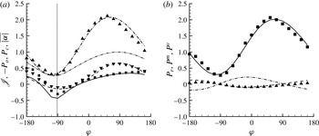
a). However, the current study requires one single set of coefficients for the analysis and comparison between different phase delays. Using all numerical simulation data with 20 different phase delays, which are denoted in figure 13, we find the set of coefficients which fit best for all cases:
 $$\begin{eqnarray}C_{T}=0.166,\quad C_{R}=1.823,\quad C_{D}(0)=0.153,\quad C_{D}({\rm\pi}/2)=3.362.\end{eqnarray}$$
Although the fitting is less accurate than the one provided by coefficients tailored for individual cases, reasonable accuracy is still maintained as is demonstrated by a similar comparison for
 ${\it\phi}=-{\rm\pi}/2$
in figure 12(b).
Figure 13 shows the time-averaged drag
 $\bar{F}_{x}$
and its three components computed by the quasi-steady model with the same coefficients and the comparison to the values directly computed by DNS with different phase delays. It is noted that the lift-induced component
 $\boldsymbol{F}^{c}$
and viscous drag component
 $\boldsymbol{F}^{{\it\nu}}$
in the numerical simulation are normal to each other and can be decoupled from the total force
 $\boldsymbol{F}$
by orthogonality, while their
 $x$
-components and averages are calculated thereafter, and the ones from the quasi-steady model are calculated directly by their definitions. For the time-averaged value in one flapping period, the added mass components are zero by definition. The agreement is in good overall with a small discrepancy near
 ${\it\phi}=-{\rm\pi}$
.
Figure 13 suggests that the lift component
 $\bar{F}_{x}^{c}$
generates thrust (i.e. negative value in the figure), and the viscous drag component
 $\bar{F}_{x}^{{\it\nu}}$
generates drag. Therefore, the optimal total force
 $\bar{F}_{x}$
(i.e. the minimum in terms of drag) is reached at a balance between
 $\bar{F}_{x}^{c}$
and
 $\bar{F}_{x}^{{\it\nu}}$
. With the change of phase delays, the variation of
 $\bar{F}_{x}^{{\it\nu}}$
is larger than the variation of
 $\bar{F}_{x}^{c}$
, so that,
 $\bar{F}_{x}^{{\it\nu}}$
becomes the dominant factor and put the priority of drag reduction in reducing the viscous drag. In fact, the vertical line marked for the optimal total force
 $\bar{F}_{x}$
is close to the phase delay for the minimum of
 $\bar{F}_{x}^{{\it\nu}}$
. When (5.10) for the viscous component is checked, the key to decrease its values is to decrease the absolute angle of attack,
 $|{\it\alpha}|$
, since
 $C_{D}(0)$
is much smaller than
 $C_{D}({\rm\pi}/2)$
in the current case. When
 $|{\it\alpha}|$
(from numerical simulation) is added to figure 13, its lowest point matches with the minimum of
 $\bar{F}_{x}^{{\it\nu}}$
(as well as the optimal phase delay). On the physical side, the small angle of attack also explains the absence of leading-edge vortices when the phase delay reaches its optimum, which has been observed earlier in figure 10.
Step 2. Optimization with a time-varying phase delay
The second step is to move from a constant phase delay to a time-varying phase delay. Taking advantage of the adjoint-based approach, the computational cost remains almost the same, although the number of control parameters increases by several orders (from one to the total number of discrete time points for one flapping period).
The initial value is chosen to be the optimal constant phase delay
 ${\it\phi}^{(1)}(t)=-77.3^{\circ }$
, which is assumed to be located in a good neighbourhood near the optimal time-varying control. To avoid numerical instability and keep the control realistic, the range of variation is limited by
 $$\begin{eqnarray}{\it\phi}^{(1)}-{\rm\Delta}{\it\phi}\leqslant {\it\phi}(t)\leqslant {\it\phi}^{(1)}+{\rm\Delta}{\it\phi},\end{eqnarray}$$
with
 ${\rm\Delta}{\it\phi}=60^{\circ }$
. The constraint is implemented by adding a penalty term to the original cost function:
 $$\begin{eqnarray}\tilde{\mathscr{J}}=\mathscr{J}+\int _{0}^{T}{\it\Theta}\left(\frac{{\it\phi}(t)-{\it\phi}^{(1)}}{{\rm\Delta}{\it\phi}}\right)\text{d}t,\end{eqnarray}$$
where
 ${\it\Theta}$
is a penalty function defined by
 $$\begin{eqnarray}{\it\Theta}(x)=\left\{\begin{array}{@{}ll@{}}{\it\beta}(x-1)^{4},\quad & x>1\\ 0,\quad & -1\leqslant x\leqslant 1\\ {\it\beta}(x+1)^{4},\quad & x<-1,\end{array}\right.\end{eqnarray}$$
with the penalty parameter
 ${\it\beta}$
being a large positive number.
After 4 iterations, the optimization algorithm reduces the drag further (from its optimum with a constant phase delay) by 53 % from
 $-0.198$
to
 $-0.303$
(figure 14
a). The optimal phase delay varies at the frequency
 $2k$
which is the same as the frequency of the drag
 $F_{x}$
, and the control is constrained by the upper limit (figure 14
b). We have tested and found that the cost can be further reduced if we move the upper limit to a larger value, however, the oscillation at larger amplitude brings in the risk of numerical instability and it may not be desirable in practice either.
Optimization for the drag reduction of a rigid flapping plate: (a) the cost function for drag reduction versus the number of iterations; (b) the optimal constant control (– – – –) and the optimal time-varying control (——), with (– ⋅ – ⋅ –) representing the upper and lower constraints.

The vortex structures of a flapping plate with the optimal time-varying phase delay for drag reduction during (a) an upstroke and (b) a downstroke.

Figure 15 shows the flow field with the optimal time-varying control. In its comparison to the flow field by the non-optimized initial control used in the previous case (figure 9) and the optimal constant control used as the initial value here (figure 10), the leading-edge vortex, instead of being removed (by the optimal constant control), is moved to the other side (the front) of the plate. The new location of the leading-edge vortex produces a low-pressure region in front of the plate which generates a large thrust force in both the upstroke and the downstroke.
Comparison of the instantaneous (a) pitch angle and (b) angle of attack with the initial (optimal constant) control (– – – –) and the optimal time-varying control (——). For reference, the plunging velocity is marked by
 $\cdots \cdots$
. In (b), the grey shaded area between lines indicates the regions where
 $|{\it\alpha}|$
decreases, and the non-shaded area indicates where
 $|{\it\alpha}|$
increases, when the control is optimized; the shaded area is also approximately boxed for easy reference.

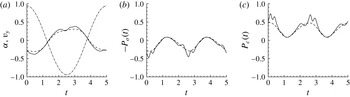
The optimization process provides a unique opportunity to understand the large improvement of aerodynamic performance brought about by a relatively small difference between the current initial (i.e. optimal constant) control and the optimal time-varying control. Instantaneous pitch angles with the initial (optimal constant) and the optimal time-varying controls are compared in figure 16(a). An obvious drop in amplitude of the pitch angle is shown when the plate is approaching the centre plan where the plunging speed reaches its maximum value. At the same time, the absolute value of the instantaneous angle of attack increases at these points as shown in figure 16(b). The large angle of attack apparently contributes to the generation of strong leading-edge vortex in the front side, shown in figure 15. During the upstroke, a large negative value of the angle of attack produces a strong anticlockwise vortex at the leading edge; during the downstroke, a large positive value of the angle of attack produces a strong clockwise vortex at the leading edge. Both contribute to the thrust.
Taking a closer look at figure 16(b), we see that the optimal time-varying control changes the angle of attack in the following manner: the absolute value of the angle of attack,
 $|{\it\alpha}|$
, is reduced when the plunging velocity magnitude is small, and it is increased when the plunging velocity magnitude is large. The quasi-steady model shown earlier can help to explain the effect of this change. Among the three force components shown in (5.7),
 $F_{x}^{c}$
is usually the main source for thrust. Since the current contribution from the angular velocity to the circulation is small, equations (5.8) and (5.9) lead to an approximation:
 $F_{x}^{c}\sim v_{y}\sin 2{\it\alpha}$
. To keep
 $F_{x}^{c}$
negative (being thrust), the signs of
 $v_{y}$
and
 ${\it\alpha}$
need to stay opposite. When the magnitude of the plunging velocity
 $|v_{y}|$
is small, an increase in
 $|{\it\alpha}|$
has a very small impact on
 $F_{x}^{c}$
. However, the impact on
 $F_{x}^{{\it\nu}}$
is much larger due to the fact that the amplitude of
 $F_{x}^{{\it\nu}}\sim v\sin ^{2}{\it\alpha}$
, derived from (5.10), stays at a reasonably large value in its
 $v_{x}$
component. On the other hand, when the magnitude of the plunging velocity
 $|v_{y}|$
is large, an increase in
 $|{\it\alpha}|$
leads to a large reduction in
 $F_{x}^{c}$
in comparison to some moderate increase in
 $F_{x}^{{\it\nu}}$
, and results in an overall drag reduction in total force
 $F_{x}$
. In other words, to reduce the total drag
 $F_{x}$
, the absolute value of angle of attack
 $|{\it\alpha}|$
needs to be reduced when the plunging speed is small but be increased when the plunging speed is large.
The above explanation is confirmed by the force history shown in figure 17. Within the boxed regions, where
 $|{\it\alpha}|$
is decreased by the optimal time-varying control, the reduction of viscous drag
 $F_{x}^{{\it\nu}}$
is greater than the increase of lift-induced drag
 $F_{x}^{c}$
. Outside the boxed regions, where
 $|{\it\alpha}|$
is increased by the optimal time-varying control, the increase of viscous drag
 $F_{x}^{{\it\nu}}$
is less than the reduction of lift-induced drag
 $F_{x}^{c}$
. So, the time-varying optimization leads to an overall reduction of total drag across almost all regions. Here, the adjoint-based optimization algorithm certainly shows the capability to find the balance between two contradictory strategies required by the force’s viscous component and lift-induced component and reveals a particular control strategy.
Comparison of the force history of (a) the lift-induced drag component
 $F_{x}^{c}$
and (b) the viscous drag component
 $F_{x}^{{\it\nu}}$
with the initial (optimal constant) control (– – – –) and the optimal time-varying control (——). The approximate regions, where
 $|{\it\alpha}|$
decreases with the optimal control, is boxed for reference. The grey shaded area between the forces indicates where the force components decrease, and the non-shaded area indicates where the force components increase, when the control is optimized.

The above discussion on plunging and pitching and their roles in propulsion coincides with the discussion by others, although the current work comes from a different perspective. Tuncer & Kaya (Reference Tuncer and Kaya2005) showed in their work that the maximum thrust generation of a flapping airfoil is achieved at a large plunging amplitude. It matches with our observation above that the plunging velocity can affect the thrust directly by contributing to the lift-induced thrust or indirectly by changing the angle of attack. Jones & Platzer (Reference Jones and Platzer1997) and Culbreth et al. (Reference Culbreth, Allaneau and Jameson2011) showed that adding the pitching motion to the plunging can greatly improve the propulsive performance. The same conclusion is indicated by our discussion on the role of pitching and its phase delay through the current optimization process. The pitching motion adjusts the angle of attack, which can either reduce directly the viscous drag component
 $F_{x}^{{\it\nu}}$
or change the circulation to decrease the lift-induced component
 $F_{x}^{c}$
. Without the pitching or the right pitching motion, all the aforementioned mechanisms for drag reduction (i.e. thrust improvement) do not exist anymore.
5.1.2 Optimization for propulsive efficiency
With other parameters staying the same, the approach is applied to study the effect of phase delay on the propulsive efficiency, which is sometimes a more important factor in practice than the thrust itself. The propulsive efficiency is defined by,
 $$\begin{eqnarray}{\it\eta}=\frac{P_{o}}{P_{c}},\end{eqnarray}$$
where
 $P_{o}$
is the useful output power for propulsion produced over one period and
 $P_{c}$
is the total consumed power over the same period:
 $$\begin{eqnarray}\left.\begin{array}{@{}c@{}}\displaystyle P_{o}=-\frac{1}{T}\int _{0}^{T}\int _{\mathscr{S}}U{\it\sigma}_{1j}n_{j}\,\text{d}s\,\text{d}t=-U\bar{F_{x}},\\ \displaystyle P_{c}=-\frac{1}{T}\int _{0}^{T}\int _{\mathscr{S}}(u_{i}-U_{i}){\it\sigma}_{ij}n_{j}\,\text{d}s\,\text{d}t,\end{array}\right\}\end{eqnarray}$$
assuming the incoming velocity
 $\boldsymbol{U}=(U,0)$
with
 $U=1$
in our non-dimensionalization.
To stay as a minimization problem for convenience, the cost function is defined by
 $$\begin{eqnarray}\mathscr{J}=-{\it\eta}.\end{eqnarray}$$
Then we find the perturbed cost function,
 $$\begin{eqnarray}\displaystyle \mathscr{J}^{\prime } & = & \displaystyle -\frac{P_{c}}{P_{c}^{2}}P_{o}^{\prime }+\frac{P_{o}}{P_{c}^{2}}P_{c}^{\prime }\nonumber\\ \displaystyle & = & \displaystyle \frac{1}{T}\int _{0}^{T}\int _{\mathscr{S}}\left[\frac{P_{c}}{P_{c}^{2}}{\it\delta}_{1i}-\frac{P_{o}}{P_{c}^{2}}(u_{i}-U_{i})\right]{{\it\sigma}^{\prime }}_{ij}n_{j}\,\text{d}s\,\text{d}t-\frac{1}{T}\int _{0}^{T}\int _{\mathscr{S}}\frac{P_{o}}{P_{c}^{2}}{u^{\prime }}_{i}{\it\sigma}_{ij}n_{j}\,\text{d}s\,\text{d}t\nonumber\\ \displaystyle & & \displaystyle +\,\frac{1}{T}\int _{0}^{T}\int _{\mathscr{S}}\left\{\left[\frac{P_{c}}{P_{c}^{2}}{\it\delta}_{1i}-\frac{P_{o}}{P_{c}^{2}}(u_{i}-U_{i})\right]\frac{\partial {\it\sigma}_{ij}}{\partial x_{j}}-\frac{P_{o}}{P_{c}^{2}}\frac{\partial u_{i}}{\partial x_{j}}{\it\sigma}_{ij}\right\}Z_{k}n_{k}\,\text{d}s\,\text{d}t,\end{eqnarray}$$
with detailed derivation being deferred to appendix A. Setting the right-hand-side term and the boundary condition for the adjoint equations:
 $$\begin{eqnarray}\left.\begin{array}{@{}c@{}}\mathscr{F}^{\ast }=0\quad \text{in}~{\it\Omega},\\ \displaystyle u_{i}^{\ast }=-\frac{P_{c}}{P_{c}^{2}}{\it\delta}_{1i}+\frac{P_{o}}{P_{c}^{2}}(u_{i}-U_{i})\quad \text{on}~\mathscr{S},\end{array}\right\}\end{eqnarray}$$
and finding the adjoint equations for
 $Z^{\ast }$
as,
 $$\begin{eqnarray}Z_{i}^{\ast }=-\!\left({\it\sigma}_{ij}^{\ast }n_{j}+u_{j}^{\ast }u_{j}n_{i}+\frac{P_{o}}{P_{c}^{2}}{\it\sigma}_{ij}n_{j}\right)\quad \text{on}~\mathscr{S}.\end{eqnarray}$$
Then we have the gradient:
 $$\begin{eqnarray}g(t)=\frac{1}{T}\int _{\mathscr{S}}Z_{k}\left[-\frac{\text{d}Z_{k}^{\ast }}{\text{d}t}-Z_{k}^{\ast }\text{div}_{\mathscr{ S}}V-Z_{i}^{\ast }\frac{\partial u_{i}}{\partial x_{k}}-\left(u_{i}^{\ast }\frac{\partial {\it\sigma}_{ij}}{\partial x_{j}}+\frac{P_{o}}{P_{c}^{2}}\frac{\partial u_{i}}{\partial x_{j}}{\it\sigma}_{ij}\right)n_{k}\right]\text{d}s.\end{eqnarray}$$
The same as the optimization process for drag reduction, the optimization for propulsive efficiency has also two steps: step one with a constant phase delay, and step two with a time-varying phase delay. The outcome of step one (i.e. the optimal constant phase delay) will serve as the initial value for the optimization in step two.
Step 1. Optimization with a constant phase delay
The cost function for propulsive efficiency versus the number of iterations.

The vortex structures of a flapping plate with the optimal constant phase delay
 ${\it\phi}=-91.27^{\circ }$
for propulsive efficiency during (a) an upstroke and (b) a downstroke.

The cost function and power components at different phase delays are plotted separately, for clarity, in (a) with the cost function
 $\mathscr{J}=-P_{o}/P_{c}$
(—— and ▪), the negative output power
 $-P_{o}$
(– – – – and ▾), the total power consumption
 $P_{c}$
(— ⋅ — and ▴), and in (b) with the individual components from the total power consumption
 $P_{c}$
: the rotational component
 $P_{r}$
(– – – – and ▴), the added mass component
 $P^{m}$
(— ⋅ —) and the viscous drag component
 $P^{{\it\nu}}$
(—— and ▪). The values are computed independently from the numerical simulation (marked by symbols) and the quasi-steady model (marked by lines). The averaged value of the absolute angle of attack
 $\overline{|{\it\alpha}|}$
(— ⋅ ⋅ —) and the optimal phase delay (vertical
 $\cdots \cdots$
) are added in (a) for reference.

For constant phase delay, we start with the same initial value:
 ${\it\phi}=-30^{\circ }$
. The optimal value
 ${\it\phi}=-91.27^{\circ }$
is reached in 2 iterations, and the cost function is reduced from 0.054 to
 $-0.320$
(figure 18). The change of sign indicates the change from drag to thrust, and more negative value indicates higher efficiency for thrust. Figure 19 shows that the flow field with the optimal control for high efficiency (
 ${\it\phi}=-91.27^{\circ }$
) has vortex structures similar to the one with the optimal constant control for drag reduction (
 ${\it\phi}=-77.3^{\circ }$
).
To understand the mechanism behind the optimization process for propulsive efficiency, the same quasi-steady model with the same coefficients in (5.11) is used for analysis. To confirm the accuracy of the quasi-steady model (with coefficients computed to best fit 20 numerical simulation cases), figure 20 compares the cost function, output power, consumed power, and individual power components computed directly by numerical simulation with the ones computed by the quasi-steady model. The agreement shown in the figure allows us to use the terms from the quasi-steady model to help with the understanding of the simulation and optimization data.
The minimization of the cost function
 $J=-P_{o}/P_{c}$
, which is defined for the increase of propulsive efficiency, can be achieved by either increasing the output power
 $P_{o}$
or decreasing the total power consumption
 $P_{c}$
. The strategy to increase the thrust output power would be similar to the one discussed earlier in § 5.1.1 to increase the thrust. Therefore, the discussion in this section is focused on the total power consumption. The total power
 $P_{c}$
can be decomposed by different motion types to the translational component
 $P_{t}$
and the rotational component
 $P_{r}$
:
 $$\begin{eqnarray}P_{c}=P_{t}+P_{r}.\end{eqnarray}$$
With different force types suggested by the quasi-steady model in (5.7), the translational power can be further decomposed to the added mass component
 $P^{m}$
, the lift-induced component
 $P^{c}$
and the viscous drag component
 $P^{{\it\nu}}$
:
 $$\begin{eqnarray}P_{t}=P^{m}+P^{c}+P^{{\it\nu}}=-\int _{0}^{T}\boldsymbol{F}^{\boldsymbol{m}}\boldsymbol{v}\,\text{d}t-\int _{0}^{T}\boldsymbol{F}^{\boldsymbol{c}}\boldsymbol{v}\,\text{d}t-\int _{0}^{T}\boldsymbol{F}^{{\bf\nu}}\boldsymbol{v}\,\text{d}t.\end{eqnarray}$$
Since the lift force is always normal to the direction of velocity, the lift-induced component
 $P^{c}$
has zero contribution and is excluded from further discussion. It is suggested in figure 20(b) that the power consumed by viscous drag
 $P^{{\it\nu}}$
is dominant, and the rotational component
 $P_{r}$
by torque and the added mass component
 $P_{m}$
are smaller and not sensitive to the change of control. Therefore,
 $P^{{\it\nu}}$
is the control priority and the focus of our analysis for total power consumption. Substituting the viscous drag force in (5.10), we find,
 $$\begin{eqnarray}P^{{\it\nu}}=\frac{1}{2}{\it\rho}_{f}l\int _{0}^{T}(C_{D}(0)\cos ^{2}{\it\alpha}+C_{D}({\rm\pi}/2)\sin ^{2}{\it\alpha})v^{3}\,\text{d}t.\end{eqnarray}$$
Since
 $C_{D}(0)$
is much smaller than
 $C_{D}({\rm\pi}/2)$
in our case, the reduction of
 $P^{{\it\nu}}$
benefits from smaller
 $|{\it\alpha}|$
, which is the same as the requirement for thrust enhancement and therefore increasing the output power
 $P_{o}$
. The analysis is confirmed by figure 20(a), where the optimal phase delay for efficiency is found in the region when
 $\overline{|{\it\alpha}|}$
is small.
The dominant role played by the viscous drag in total power consumption suggests a general strategy to improve propulsive efficiency by simply reducing the viscous drag. In later discussion on the optimization of a flexible plate, both changes of shape deformation and Reynolds number can be observed to contribute to better efficiency.
Step 2. Optimization with a time-varying phase delay
Optimization for the propulsive efficiency of a rigid flapping plate: (a) the cost function for propulsive efficiency changes by the number of iterations: (b) the optimal constant control (– – – –) and the optimal time-varying control (——), with (– ⋅ – ⋅ –) representing the upper and lower constraints.

Using the optimal constant phase delay
 ${\it\phi}^{(1)}(t)=-91.27^{\circ }$
as the initial value, the optimization can go further if variation in time is allowed. The control is limited by the same constraint:
 $$\begin{eqnarray}{\it\phi}^{(1)}-{\rm\Delta}{\it\phi}\leqslant {\it\phi}(t)\leqslant {\it\phi}^{(1)}+{\rm\Delta}{\it\phi},\end{eqnarray}$$
with
 ${\rm\Delta}{\it\phi}=60^{\circ }$
. Different form the drag reduction case, time-varying condition only push the cost function by another 8.1 % reduction from
 $-0.320$
to
 $-0.346$
after 5 iterations (figure 21). The time variation of the phase delay also stops far before it reaches the constraint.
The vortex structures of a flapping plate with the optimal time-varying phase delay for propulsive efficiency during (a) an upstroke and (b) a downstroke.

The flow field with the optimal time-varying control, as shown in figure 22, is similar to the one under the optimal constant control. The time variation seems to allow the flow to push a little more to the limit of boundary separation right before vortex shedding starts. Similar behaviour has been observed in the studies by Tuncer & Kaya (Reference Tuncer and Kaya2005) and Culbreth et al. (Reference Culbreth, Allaneau and Jameson2011).
Comparison of (a) the angle of attack
 ${\it\alpha}$
, (b) the negative of output power
 $-P_{o}$
, and (c) the total consumed power
 $P_{c}$
by the optimal constant control (– – – –) and the optimal time-varying control (——). The plunging velocity
 $v_{y}$
(— ⋅ —) is added in (a) for reference.

A detailed comparison is shown in figure 23. The optimal constant phase delay has taken most of the benefit at small
 $|{\it\alpha}|$
to simultaneously satisfy the increase of output power and the decrease of power consumption, thus it is hard for the phase delay alone, even with time variation, to push this part further without touching other parameters such as the pitching amplitude. So, some small change made by allowing time variation happens in the large
 $|v_{y}|$
region (figure 23
a). However, in this region, the increase of
 $|{\it\alpha}|$
leads to the decrease of
 $-P_{o}$
(the increase of the absolute value of output power) and the increase of
 $P_{c}$
. As a result, the effort made by the time variation shows much less impact on the propulsive efficiency.
5.2 Optimization of a flapping flexible plate
Wing flexibility has long been observed in nature’s flyers. Its effect on aerodynamic performance has attracted many research works in recent years. For example, in their numerical study of hovering flight, Vanella et al. (Reference Vanella, Fitzgerald, Preidikman, Balaras and Balachandran2009) found that wing deformation helps to increase lift-to-drag and lift-to-power ratios; Eldredge, Toomey & Medina (Reference Eldredge, Toomey and Medina2010) studied the flexibility of a flapping plate and found that flexibility reduces the sensitivity of the lift to the phase delay between the pitching and plunging motion. In this section, flexibility is added to the flapping plate, and the analysis of its aerodynamic effect is undertaken via a comparison of the optimal and non-optimal solutions.
The flexible flapping plate has a combined motion with plunging, pitching and deformation. The plate has non-dimensional length
 $l=1$
, thickness (before deformation)
 $h=0.1$
. The trajectory of its centreline is defined by
 $$\begin{eqnarray}\boldsymbol{x}=y_{0}\sin ({\it\omega}t)\boldsymbol{I}+\mathscr{R}({\it\theta})\left(\boldsymbol{X}+\mathop{\sum }_{k=1}^{n}a_{k}\sin ({\it\omega}t+{\it\varphi}_{k}){\it\psi}_{k}(X)\boldsymbol{I}\right),\end{eqnarray}$$
where
 $$\begin{eqnarray}\boldsymbol{I}=(0,1),\quad \mathscr{R}({\it\theta})=\left[\begin{array}{@{}cc@{}}\cos {\it\theta} & -\text{sin}{\it\theta}\\ \sin {\it\theta} & \cos {\it\theta}\end{array}\right],\quad {\it\theta}=a_{0}\sin ({\it\omega}t+{\it\varphi}_{0}),\end{eqnarray}$$
and
 $\boldsymbol{x}=(x,y)$
and
 $\boldsymbol{X}=(X,Y)$
are the locations of solid points described respectively in Eulerian coordinates and in the undeformed Lagrangian coordinates. The first term in (5.26) represents the plunging motion, where the plunging amplitude
 $y_{0}$
and frequency
 ${\it\omega}=2k{\rm\pi}$
are the same as those used earlier for the rigid plate. The second term represents the pitching motion, which has its rotational centre moved to the leading end of the plate. The shift of the rotational centre allows to use the eigenmodes of a cantilevered Euler–Bernoulli beam as basis functions to describe the deformation. The remaining terms are for deformation, which is defined by a summation of eigenmodes:
 $$\begin{eqnarray}\displaystyle {\it\psi}_{k}(X) & = & \displaystyle C_{k}\left[\cosh {\it\beta}_{k}X-\cos {\it\beta}_{k}X\right.\nonumber\\ \displaystyle & & \displaystyle \left.+\,\frac{\cosh {\it\beta}_{k}X+\cos {\it\beta}_{k}X}{\sinh {\it\beta}_{k}X+\sin {\it\beta}_{k}X}(\sin {\it\beta}_{k}X-\sinh {\it\beta}_{k}X)\right],\end{eqnarray}$$
where
 ${\it\beta}_{k}$
is the
 $k$
th solution of
 $$\begin{eqnarray}\cosh ({\it\beta}_{k}L)\cos ({\it\beta}_{k}L)+1=0,\end{eqnarray}$$
and
 $C_{k}$
is the normalized coefficient to satisfy the condition:
 $\max \{|{\it\psi}_{k}(X)|\}=1$
.
The control for a flexible flapping plate is then defined by
 $$\begin{eqnarray}{\it\phi}=\{a_{0},{\it\varphi}_{0},\ldots ,a_{n},{\it\varphi}_{n}\},\end{eqnarray}$$
where
 $\{a_{0},{\it\varphi}_{0}\}$
are the amplitude and phase delay of the rigid body pitching motion, and
 $\{a_{n},{\it\varphi}_{n}\}$
(
 $n>0$
) are the amplitude and phase delay of each eigenmodes for deformation. The deformation is limited by
 $$\begin{eqnarray}|a_{n}|\leqslant 0.5,\quad \text{for}~n>0.\end{eqnarray}$$
The control is optimized first for drag reduction and then for propulsive efficiency.
5.2.1 Optimization for drag reduction
Following the same derivation shown in § 5.1 and using the same source term and boundary conditions for the adjoint system (but for a more complex control including flexibility), the gradient leading to drag reduction of a flexible flapping plate is given by,
 $$\begin{eqnarray}\displaystyle g_{l}=\frac{\partial \mathscr{J}}{\partial {\it\phi}_{l}}=\frac{1}{TD_{0}}\int _{0}^{T}\int _{\mathscr{S}}\left[Z_{k,l}\frac{\partial {\it\sigma}_{1j}}{\partial x_{j}}n_{k}-\left(\dot{V}_{i,l}-Z_{k,l}\frac{\partial u_{i}}{\partial x_{k}}\right)Z_{i}^{\ast }\right]\text{d}s\,\text{d}t, & & \displaystyle\end{eqnarray}$$
where
 $$\begin{eqnarray}\displaystyle \dot{V}_{i,l}=\frac{\partial V_{i}}{\partial {\it\phi}_{l}},\quad Z_{i,l}=\frac{\partial S_{i}}{\partial {\it\phi}_{l}},\quad Z_{i}^{\ast }={\it\sigma}_{ij}^{\ast }n_{j}+u_{j}^{\ast }u_{j}n_{i}, & & \displaystyle\end{eqnarray}$$
and
 $S_{i}$
is the solid boundary location.
The optimization has been applied to different Reynolds numbers:
 $Re=300$
and
 $Re=100$
, and different levels of flexibility:
 $n=0$
for a rigid plate,
 $n=1$
having only the first eigenmode for deformation,
 $n=2$
having both the first and the second eigenmodes for deformation. For all cases, the same initial control (case 0) is given by
 $$\begin{eqnarray}{\it\phi}=\{0.475,-{\rm\pi}/6,0,0,\ldots ,0,0\},\end{eqnarray}$$
which has a pitching amplitude 0.475 with phase delay
 $-{\rm\pi}/6$
and zero flexibility (i.e. rigid). Details on parameters and outcomes are listed in table 1.
The history of drag forces in one period for case 1 (——), case 2 (– – – –), case 3 (— ⋅ —) and case 4 (
 $\cdots \cdots$
) of Group I (
 $Re=300$
).

Optimization results for drag reduction with different Reynolds numbers and flexibility: cases 0 has the initial control; cases 1, 2 and 3 have the optimal controls with different levels of flexibility; case 4 (of Group I) is a reference case, which removes all flexibility terms from case 3 (of Group I) and keeps the rigid plunging and pitching motion the same.

It is shown in table 1 that the adjoint-based optimization provides solutions for all cases to change from drag to thrust (and to larger thrust). The comparison between the rigid plate (case 1) and the flexible plates (case 2 and 3) shows significant contribution from the flexibility to the thrust improvement. At Reynolds number 300 (Group I), the optimal flexible plate (case 3) provides 111 % more thrust than the rigid plate (case 1); at lower Reynolds number 100 (Group II), the impact is even more dramatic with 1069 % more thrust from the rigid plate (case 1) to the flexible plate (case 3). For both Reynolds numbers, a higher level of flexibility (case 3, with 2 eigenmodes) provides more thrust than a lower level of flexibility (case 2, with 1 eigenmode). It is worth noting that the thrust brought in by more flexibility comes with some small cost of efficiency, since the propulsive efficiency is not part of the cost function at this moment.
The current study also shows that flexibility helps to reduce the sensitivity of the propulsion performance to the Reynolds number. For a rigid plate (
 $n=0$
), the optimal thrust is reduced by 86.5 % from 0.26 to 0.035 when the Reynolds number changes from 300 to 100; for a flexible plate (
 $n=2$
), the optimal thrust is only reduced by 25.5 % from 0.549 to 0.409. It suggests that flexibility helps to maintain the aerodynamic performance in complex environment with variable Reynolds number (e.g. flow with gust), and flexibility also plays a more significant role in lower Reynolds number region such as flapping-wing flight of insects.
Comparison of kinematics, deformation and vortex structures of (a) the rigid plate (case 1), (b) the plate with small deformation (case 2), (c) the plate with large deformation (case 3) and (d) the reference (case 4), with
 $Re=300$
(Group I), at
 $t=0$
, 1 and 1.5.

For detailed comparison, figure 24 shows the history of drag forces for the optimal rigid plate (case 1), the optimal plate with small deformation (case 2), the optimal plate with large deformation (case 3) and the reference rigid plate (case 4, by removing the flexibility directly from case 3) for
 $Re=300$
(Group I). Among the half-cycle, the one with small deformation (case 2) reduces the drag by a small amount near
 $t=0$
and
 $t=1.5$
; the one with large deformation (case 3) reduces the drag by a large amount near
 $t=0$
with a slight increase near
 $t=1$
; the reference (case 4) keeps the same or even better drag reduction at
 $t=0$
but cannot maintain the same saving later, instead it adds large drag for
 $1<t<2$
.
Figure 25 shows visually the flapping kinematics, deformation and vortex structures for better understanding of the control mechanism. Flexibility, especially large deformation, allows the plate to have a large angle of attack and hold the leading-edge vortex to the front for the benefit of lift-induced thrust, while the overall profile stays small (by deformation) to avoid an increase in viscous drag. It is obvious that the reference case 4, which keeps the same pitching (i.e. angle of attack) at the leading edge but removes all the deformations, has the same benefit from the lift-induced thrust (near
 $t=0$
) but adds a huge amount of viscous drag later.
5.2.2 Optimization for propulsive efficiency
The adjoint-based optimization is applied in this section to understand the effect of flexibility on propulsive efficiency. Following the same derivation shown in § 5.1.2 and using the same source term and boundary conditions for the adjoint system (but again for a more complex control), the gradient leading to better propulsive efficiency for a flexible plate is given by,
 $$\begin{eqnarray}\displaystyle g_{l} & = & \displaystyle \frac{1}{T}\int _{0}^{T}\int _{\mathscr{S}}\left[-Z_{k,l}\left(u_{i}^{\ast }\frac{\partial {\it\sigma}_{ij}}{\partial x_{j}}+\frac{P_{o}}{P_{c}^{2}}\frac{\partial u_{i}}{\partial x_{j}}{\it\sigma}_{ij}\right)n_{k}\right.\nonumber\\ \displaystyle & & \displaystyle \left.-\left(\dot{V}_{i,l}-Z_{k,l}\frac{\partial u_{i}}{\partial x_{k}}\right)Z_{i}^{\ast }\right]\,\text{d}s\,\text{d}t,\end{eqnarray}$$
where
 $$\begin{eqnarray}\dot{V}_{i,l}=\frac{\partial V_{i}}{\partial {\it\phi}_{l}},\quad Z_{i,l}=\frac{\partial S_{i}}{\partial {\it\phi}_{l}},\quad Z_{i}^{\ast }={\it\sigma}_{ij}^{\ast }n_{j}+u_{j}^{\ast }u_{j}n_{i}+\frac{P_{o}}{P_{c}^{2}}{\it\sigma}_{ij}n_{j},\end{eqnarray}$$
and
 $S_{i}$
is the solid boundary location.
Optimization results for propulsive efficiency with different Reynolds numbers and flexibility: case 0 has the initial control; cases 1, 2 and 3 have the optimal controls with different levels of flexibility; case 4 (of Group III) is a reference case, which removes all flexibility terms from case 3 (of Group III) and keeps the rigid plugging and pitching motion the same.

Similar to the cases for drag reduction, all cases are grouped by different Reynolds numbers
 $Re=300$
(Group III) and
 $Re=100$
(Group IV); within one group, different cases for different flexibility (
 $n=0$
, 1 and 2) are studied. The same initial condition in (5.34) is used. Detailed information is in table 2.
It is shown that flexibility helps to improve propulsive efficiency in a substantial way. At a Reynolds number of 300 (Group III), the optimal flexible plate (case 3) increases the propulsive efficiency by 52.6 % from the optimal rigid plate (case 1); at a lower Reynolds number of 100 (Group IV), the change in efficiency is a dramatic 595 % from 0.022 (case 1) to 0.153 (case 3). The comparison between small flexibility (case 2) and large flexibility (case 3) shows that a higher level of flexibility provides significant efficiency improvement at low Reynolds number
 $Re=100$
, but such impact is negligible at higher Reynolds number
 $Re=300$
.
Similar to thrust performance, flexibility also helps reduce the sensitivity to Reynolds number for propulsive efficiency. For a rigid plate (
 $n=0$
), the optimal propulsive efficiency is reduced by 91.2 % from 0.247 to 0.022 when the Reynolds number changes from 300 to 100; for a flexible plate (
 $n=2$
), the reduction is 59.4 % from 0.377 to 0.153. It suggests the importance of including flexibility in complex flow environment and especially at low Reynolds number.
The history of (a) drag forces and (b) total power consumption for case 1 (——), case 2 (– – – –), case 3 (— ⋅ —) and case 4 (
 $\cdots \cdots$
) of Group III (
 $Re=300$
).

Comparison of kinematics, deformation and vortex structures of (a) the rigid plate (case 1), (b) the plate with small deformation (case 2), (c) the plate with large deformation (case 3) and (d) the reference (case 4), with
 $Re=300$
(Group III), at
 $t=0$
, 1 and 1.5.

The history of drag forces and total power consumption, shown in figure 26, indicate that the strategy adopted by the optimal control is to push for lower drag (i.e. higher thrust) while keeping the same level of overall power consumption. With overall better thrust performance, there is some increase of power consumption at the beginning of the upstroke and downstroke, but it is mostly balanced out by the decrease at other places. The damage of forcing the flexibility out in case 4 is more obvious, since the increase of viscous drag not only removes the benefit of output power but also adds a huge overload to the total power consumption.
There is actually a clear difference between the current optimization and the previous drag reduction case, which is shown by the flow field plotted in figure 27. Instead of holding a large leading-edge vortex to provide more benefit for lift-induced thrust, all leading-edge vortices are suppressed in the current optimization for propulsive efficiency. As we have learned from the quasi-steady model in earlier discussions, viscous drag plays a big negative role in propulsive efficiency. So the increase of overall profile by allowing a large leading-edge vortex turns out to be too high a price to pay for efficiency optimization, despite its benefit in thrust improvement.
5.3 Optimization of a three-dimensional plate in hovering motion
It is a natural extension for the study to move from a two-dimensional plate to a three-dimensional plate. We choose the same rigid plate in hovering motion, which has been studied extensively by Trizila et al. (Reference Trizila, Kang, Aono, Shyy and Visbal2011), as our base case. The plate used in the work of Trizila et al. (Reference Trizila, Kang, Aono, Shyy and Visbal2011) has an aspect ratio,
 $AP=4$
, and Reynolds number,
 $Re=100$
. With initial numerical simulations combined with surrogate modelling, they achieved the complete map of a three-parameter design space including: the amplitude of translational motion, the amplitude and the phase delay of rotational motion. Such a space exploration is important for some cases. However, an adjoint-based optimization could be much more efficient if optimization is the major concern and the result is more accurate without involving a surrogate model. In the first case below, we take the same parameters for the optimization of the lift coefficient. Although adjoint-based optimization is known for its efficiency and the fact that it is model free, it has the same risk as other gradient-based approaches, which is the possibility of being trapped by a local minimum. This comparison of optimal solutions by an adjoint approach and a parameter study helps to check this risk in applying the adjoint-based approach to a flapping-wing study and also serves as a benchmark. In the second case, we include chordwise flexibility in the optimization to understand the impact from flexibility to a hovering plate.
5.3.1 Optimization of a rigid plate
Sketch of a three-dimensional hovering plate.

As shown in figure 28, we use a flat rectangle plate which translates along the
 $x$
axis and rotates about the
 $z$
axis with the motion defined by
 $$\begin{eqnarray}\left.\begin{array}{@{}c@{}}x(t)=x_{0}\sin (2{\rm\pi}kt),\\ {\it\theta}(t)={\it\theta}_{0}-{\it\theta}_{{\it\alpha}}\sin (2{\rm\pi}kt+{\it\varphi}),\end{array}\right\}\end{eqnarray}$$
where
 $k$
is the flapping frequency,
 $x_{0}$
is the translational amplitude and
 ${\it\theta}_{{\it\alpha}}$
and
 ${\it\varphi}$
are the amplitude and phase delay of the rotational motion with equilibrium angle
 ${\it\theta}_{0}=90^{\circ }$
(Trizila et al.
Reference Trizila, Kang, Aono, Shyy and Visbal2011). The plate shape is defined by the cord length
 $c$
as
 $4c\times c\times 0.08c$
. It is noted that our plate is slightly thicker than the one used by Trizila et al. (Reference Trizila, Kang, Aono, Shyy and Visbal2011) (
 $0.02c$
) to meet the need of efficiency for the immersed boundary approach used for this study. The impact from the smaller thickness is tested to be small in our study, and such small influence from the fine detail of the plate shape on its aerodynamic performance has also been suggested by Trizila et al. (Reference Trizila, Kang, Aono, Shyy and Visbal2011). The Reynolds number is defined by
 $$\begin{eqnarray}Re=\frac{U_{ref}L_{ref}}{{\it\nu}},\end{eqnarray}$$
where the reference length
 $L_{ref}$
is the chord length
 $c$
, and the reference velocity
 $U_{ref}$
is the maximum translational velocity,
 $U_{ref}=2{\rm\pi}kx_{0}$
. The constant
 $U_{ref}$
implies that the flapping frequency
 $k$
is a function of
 $x_{0}$
. In our simulation, we keep the Reynolds number at 100, and optimize three kinematic parameters
 $x_{0}$
,
 ${\it\theta}_{{\it\alpha}}$
and
 ${\it\varphi}$
in a parametric space defined in table 3, which is the same design space explored by Trizila et al. (Reference Trizila, Kang, Aono, Shyy and Visbal2011).
The range of control variables for lift optimization.

To increase the lift coefficient, we use a cost function,
 $$\begin{eqnarray}\mathscr{J}=-\frac{1}{D_{0}}\int _{0}^{1}\int _{\mathscr{S}}{\it\sigma}_{2j}n_{j}\,\text{d}s\,\text{d}\hat{t},\end{eqnarray}$$
where
 $D_{0}=1/2{\it\rho}U_{ref}^{2}A$
,
 $A$
is the total plate area, and a new time scale
 $\hat{t}=t/T$
is used to avoid the change of time range when the control parameter
 $x_{0}$
(as well as the frequency
 $k$
) is changed during the optimization process. Choosing the source term and boundary conditions for the adjoint system,
 $$\begin{eqnarray}\left.\begin{array}{@{}c@{}}\mathscr{F}^{\ast }=0\quad \text{in}~{\it\Omega},\\ u_{i}^{\ast }=-{\it\delta}_{2i}\quad \text{on}~\mathscr{S},\end{array}\right\}\end{eqnarray}$$
we find the gradient,
 $$\begin{eqnarray}\displaystyle g_{l}=\frac{\partial \mathscr{J}}{\partial {\it\phi}_{l}}=-\frac{1}{D_{0}}\int _{0}^{1}\int _{\mathscr{S}}\left[Z_{k,l}\frac{\partial {\it\sigma}_{2j}}{\partial x_{j}}n_{k}-\left(\dot{V}_{i,l}-Z_{k,l}\frac{\partial u_{i}}{\partial x_{k}}\right)Z_{i}^{\ast }\right]\text{d}s\hat{t}, & & \displaystyle\end{eqnarray}$$
where
 $$\begin{eqnarray}\displaystyle \dot{V}_{i,l}=\frac{\partial V_{i}}{\partial {\it\phi}_{l}},\quad Z_{i,l}=\frac{\partial S_{i}}{\partial {\it\phi}_{l}},\quad Z_{i}^{\ast }={\it\sigma}_{ij}^{\ast }n_{j}+u_{j}^{\ast }u_{j}n_{i}. & & \displaystyle\end{eqnarray}$$
Table 4 shows respectively the initial control and its optimal value after 4 main iterations. The lift coefficient is improved from 0.338 to 0.620 by 83.4 %. A closer comparison shows that our optimal values match well with the high-lift region shown in the contour map provided by the design space exploration through surrogate modelling in Trizila et al. (Reference Trizila, Kang, Aono, Shyy and Visbal2011).
The trajectory of a rigid hovering plate with (a) the initial control and (b) the optimal control. The plates are highlighted for the times:
 $\hat{t}=-0.2$
, 0 and 0.2.

The time history of the lift coefficients for a rigid hovering plate with the initial control (– – – –) and the optimal control (——).

Comparison of the initial and the optimal controls and the resulting lift coefficients for a rigid hovering plate.

The
 $z$
-component of vorticity at the middle plane (
 $z=0$
) for a rigid hovering plate with (a) the initial control and (b) the optimal control at different time moments.

The pressure distribution of a rigid hovering plate with (a) the initial control and (b) the optimized control on the lower (left) and upper (right) surfaces at different time moments.

The vortex structures (shown by an isosurface of
 $Q=0.015$
) of a rigid hovering plate with (a) the initial control and (b) the optimal control at different time moments.

Figures 29 and 30 compare the motion and time history of lift coefficients with the initial and the optimal controls. For both cases, there are two peaks of lift during one half-cycle. The first peak occurs at
 $\hat{t}=-0.2$
and is caused by the interaction of the plate with the vortex pair shedding from the previous half-cycle, as shown in figure 31. The second peak (lift maximum) occurs at
 $\hat{t}=0$
, where the plate has its largest translation velocity. Compared to the initial control, the plate with the optimal control has a larger angle of attack at
 $\hat{t}=0$
. This generates a stronger leading-edge vortex (figure 31), which causes large pressure difference in upper and lower surface of the plate (figure 32) and produces larger lift. At
 $\hat{t}=0.2$
, in the case with the initial control, the vortex pair generates a momentum on the plate’s upper surface (figure 31), therefore it produces downward force (figure 32). On the other hand, the plate with the optimal control has an advanced rotation. The momentum induced by the vortex pair acts on the plate’s lower surface, thus generating lift instead. These results suggest that, in hovering flight, both the plunging/pitching and the wake capture are important for lift generation. The timing of the plate interacting with the wake is closely related to the phase delay. The vortex structures depicted in figure 33 by an isosurface of Q criterion (Hunt, Way & Moin Reference Hunt, Way and Moin1988) clearly show much stronger downwash from the optimal motion for the increase of lift performance.
5.3.2 Optimization of a flexible plate
The efficiency of an adjoint-based approach allows us to introduce more control parameters without adding extra expense. To take this advantage, we introduced deformation to the study of a hovering plate. At this moment, we only consider the chordwise deformation, which is defined in a similar manner as in the two-dimensional case by the first eigenmode described in (5.28). The ranges of the deformation amplitude
 $a_{1}$
and phase delay
 ${\it\varphi}_{1}$
are
 $-0.3\leqslant a_{1}\leqslant 0.3$
and
 $-90^{\circ }\leqslant {\it\varphi}_{1}\leqslant 90^{\circ }$
.
Comparison of the initial and the optimal controls and the resulting lift coefficients for a flexible hovering plate.

The trajectory of a flexible hovering plate with (a) the initial control and (b) the optimal control. The plates are highlighted for time moments:
 $\hat{t}=-0.05$
, 0 and 0.2.

The time history of the lift coefficients for a flexible hovering plate with the initial control (– – – –) and the optimal control (——).

The
 $z$
-component of vorticity at the middle plane (
 $z=0$
) for a flexible hovering plate with (a) the initial control and (b) the optimal control at different time moments.

The pressure distribution of a flexible hovering plate with (a) the initial control and (b) the optimized control on the lower (left) and upper (right) surfaces at different time moments.

The vortex structures (shown by an isosurface of
 $Q=0.015$
) of a flexible hovering plate with (a) the initial control and (b) the optimized control at different time moments.

Shown in table 5, the initial control of the case for a flexible plate is chosen to be the optimal control achieved earlier for the rigid plate (with zero deformation). By some moderate deformation, the lift coefficient is pushed from 0.62 to 0.88 for another 42 % increase.
Figure 34 compares the plate motion and deformation before and after the optimization. The plate is deformed in a way which shows clear ‘cupping’ towards the centre for the increase of mass flow downwash and the overall lift in turn. When the time history of the lift coefficient is compared in figure 35, we can see that the improvement mainly occurs near
 $\hat{t}=-0.05$
. Figure 36 shows that the deformation at
 $\hat{t}=-0.05$
increases the angle of attack and thus induces a stronger leading-edge vortex. This leading-edge vortex contributes to the low-pressure region on the plate’s upper surface, as shown in figure 37. Meanwhile the deformation towards the flow traps more fluid in a smaller region and increases the pressure on the lower surface. Both contribute to the larger pressure difference for lift generation (figure 37). At
 $\hat{t}=0.2$
, the plate is deformed upward and has more projection area along the vertical direction, which results in a stronger jet flow from vortex shedding and moves the shedding direction downward for the benefit of lift increase. The larger projection area also contributes to a slightly larger pressure difference between the upper and lower surfaces for stronger lift. The three-dimensional vortex structures plotted in figure 38 are clearly much stronger and clearer for a larger downwash, leading to lift increase.
6 Conclusions
Using non-cylindrical calculus, we have developed a continuous approach for adjoint-based optimization to be applied on Navier–Stokes equations with a moving boundary or morphing domain. The optimization approach provides a unique perspective for the understanding of the kinematics and deformation of a flapping wing and their effects on aerodynamic performance.
To handle the moving boundary in the adjoint derivation, non-cylindrical calculus leads to a formulation equivalent to the one derived by the traditional and more straightforward unsteady mapping function. However, the derivation using non-cylindrical calculus is much easier and the resulting formulation is simpler as well. In fact, for most cases, the unsteady mapping function is too complex to be feasibly derived. One advantage of using the continuous approach is its independence of specific numerical algorithms and simulation codes, thus it provides flexibility in numerical implementation. The other advantage is that the equations derived by the continuous approach provide some level of physical insight. To be assured of the accuracy of our derivation, both the optimal control and the local gradient information are carefully validated.
For the two-dimensional configuration, the adjoint-based optimization is applied on a rigid flapping plate and a flexible flapping plate for drag reduction and for propulsive efficiency. The rigid plate has a combined plunging and pitching motion with an incoming flow, the control parameter is the phase delay which is considered first as a constant and then as a time-varying function. It is noted that the time-varying control has more degree of freedom but the same cost by the nature of an adjoint-based algorithm. It is indicated by the optimal control that the strategy of adjusting the phase delay for thrust performance, while keeping opposite signs for the angle of attack and the plunging velocity, works to increase the angle of attack magnitude when the plunging speed is large to focus on the enhancement of lift-induced thrust, and works to decrease the angle of attack magnitude when the plunging speed is small to focus on the reduction of viscous drag. When propulsive efficiency is considered, the reduction of viscous drag takes a more dominant role because of its impact on overall power consumption. The mechanism to increase power output generally works against the mechanism to reduce the total power consumption, keeping the viscous drag in check becomes the key to finding a balance between the two mechanisms for optimization.
The flexible plate has plunging, pitching and deformation which is defined by the first two eigenmodes from structural analysis. With the same optimization goals, the control is instead the amplitude and phase delay of the pitching, the first eigenmode and the second eigenmode. When the optimal solutions with different levels of flexibility are compared, it becomes obvious that flexibility increases thrust performance by holding a strong leading-edge vortex to the front for more lift-induced drag while keeping a small profile to reduce viscous drag. However, for propulsive efficiency, again because of the critical role played by viscous drag, holding a large leading-edge vortex is no longer an option with its cost on viscous drag. It is also interesting to note that the flexibility plays a more important role for lower Reynolds number. For both drag reduction and propulsive efficiency, flexibility largely reduces the sensitivity to Reynolds number and allows a flapping wing at low Reynolds number to enjoy the high aerodynamic performance existing in the higher Reynolds number regime.
Finally, for a three-dimensional configuration, we apply the adjoint-based optimization to a plate in hovering motion, where both rigid and flexible cases are considered. The optimal control achieved for a rigid plate matches well with a similar study in literature using surrogate modelling for the exploration of the same design space. The advanced rotation in the optimal setting provides results with better wake capturing and therefore a more favourable downwash leading to lift increase. We eventually take the study to a flexible plate by introducing the amplitude and phase delay of chordwise deformation. The flexible case is able to push the lift coefficient higher by ‘cupping’ more fluid on the lower surface and deforming to larger vertical projection profile which lead to an even stronger downwash as well as larger pressure difference between the upper and lower surfaces of the plate, both for lift benefit.
Acknowledgements
The authors gratefully acknowledge the support from Air Force Office of Scientific Research (AFOSR) and U.S. Army Research Laboratory (ARL) through MAST-CTA and AHPCRC.
Appendix A. The shape derivatives of drag and power
The follow identities are useful for the derivation on the moving domain:
 $$\begin{eqnarray}\left.\begin{array}{@{}c@{}}\displaystyle \frac{\text{d}}{\text{d}t}\left(\int \int _{{\it\Omega}(t)}f\,\text{d}\boldsymbol{x}\,\text{d}t\right)=\int \int _{{\it\Omega}(t)}\frac{\partial f}{\partial t}\,\text{d}\boldsymbol{x}\,\text{d}t-\int \int _{\mathscr{S}}fV_{i}n_{i}\,\text{d}s\,\text{d}t,\\ \displaystyle \left(\int \int _{{\it\Omega}({\it\phi})}f\,\text{d}\boldsymbol{x}\,\text{d}t\right)^{\prime }=\int \int _{{\it\Omega}({\it\phi})}f^{\prime }\,\text{d}\boldsymbol{x}\,\text{d}t-\int \int _{\mathscr{S}}fZ_{i}n_{i}\,\text{d}s\,\text{d}t,\end{array}\right\}\end{eqnarray}$$
where the normal direction
 $n_{i}$
points from solid to fluid at
 $\mathscr{S}$
.
For drag reduction, the cost function is
 $$\begin{eqnarray}\displaystyle \mathscr{J} & = & \displaystyle \frac{1}{TD_{0}}\int _{0}^{T}\int _{\mathscr{S}}{\it\sigma}_{1j}n_{j}\,\text{d}s\,\text{d}t\nonumber\\ \displaystyle & = & \displaystyle \frac{1}{TD_{0}}\left(\int _{0}^{T}\int _{\mathscr{S}_{\infty }}{\it\sigma}_{1j}n_{j}\,\text{d}s\,\text{d}t-\int _{0}^{T}\int _{{\it\Omega}(t)}\frac{\partial {\it\sigma}_{1j}}{\partial x_{j}}\,\text{d}\boldsymbol{x}\,\text{d}t\right),\end{eqnarray}$$
where the normal direction
 $n_{j}$
on
 $\mathscr{S}_{\infty }$
points towards far field. The shape derivative of the cost function is then given by
 $$\begin{eqnarray}\displaystyle \mathscr{J}^{\prime } & = & \displaystyle \frac{1}{TD_{0}}\int _{0}^{T}\int _{\mathscr{S}_{\infty }}{\it\sigma}_{1j}^{\prime }n_{j}\,\text{d}s\,\text{d}t\nonumber\\ \displaystyle & & \displaystyle -\,\frac{1}{TD_{0}}\left(\int _{0}^{T}\int _{{\it\Omega}(t)}\frac{\partial {\it\sigma}_{1j}^{\prime }}{\partial x_{j}}\,\text{d}\boldsymbol{x}\,\text{d}t-\int _{0}^{T}\int _{\mathscr{S}}\frac{\partial {\it\sigma}_{1j}}{\partial x_{j}}Z_{k}n_{k}\,\text{d}s\,\text{d}t\right)\nonumber\\ \displaystyle & = & \displaystyle \frac{1}{TD_{0}}\int _{0}^{T}\int _{\mathscr{S}}\left({\it\sigma}_{1j}^{\prime }n_{j}+\frac{\partial {\it\sigma}_{1j}}{\partial x_{j}}Z_{k}n_{k}\right)\,\text{d}s\,\text{d}t.\end{eqnarray}$$
For the efficiency optimization, the form of
 $P_{o}$
is similar to the drag force, therefore we only derive the shape derivative for
 $P_{c}$
here. The consumed power is
 $$\begin{eqnarray}\displaystyle P_{c} & = & \displaystyle -\frac{1}{T}\int _{0}^{T}\int _{\mathscr{S}}(u_{i}-U_{i}){\it\sigma}_{ij}n_{j}\,\text{d}s\,\text{d}t\nonumber\\ \displaystyle & = & \displaystyle -\frac{1}{T}\int _{0}^{T}\int _{\mathscr{S}_{\infty }}(u_{i}-U_{i}){\it\sigma}_{ij}n_{j}\,\text{d}s\,\text{d}t+\frac{1}{T}\int _{0}^{T}\int _{{\it\Omega}(t)}\frac{\partial (u_{i}-U_{i}){\it\sigma}_{ij}}{\partial x_{j}}\,\text{d}\boldsymbol{x}\,\text{d}t,\end{eqnarray}$$
providing its shape derivative,
 $$\begin{eqnarray}\displaystyle P_{c}^{\prime } & = & \displaystyle -\frac{1}{T}\int _{0}^{T}\int _{\mathscr{S}_{\infty }}[(u_{i}-U_{i}){\it\sigma}_{ij}]^{\prime }n_{j}\,\text{d}s\,\text{d}t\nonumber\\ \displaystyle & & \displaystyle +\,\frac{1}{T}\int _{0}^{T}\int _{{\it\Omega}(t)}\frac{\partial [(u_{i}-U_{i}){\it\sigma}_{ij}]^{\prime }}{\partial x_{j}}d\boldsymbol{x}dt-\frac{1}{T}\int _{0}^{T}\int _{\mathscr{S}}\frac{\partial (u_{i}-U_{i}){\it\sigma}_{ij}}{\partial x_{j}}Z_{k}n_{k}\,\text{d}s\,\text{d}t\nonumber\\ \displaystyle & = & \displaystyle -\frac{1}{T}\int _{0}^{T}\int _{\mathscr{S}}u_{i}^{\prime }{\it\sigma}_{ij}n_{j}\,\text{d}s\,\text{d}t\nonumber\\ \displaystyle & & \displaystyle -\,\frac{1}{T}\int _{0}^{T}\int _{\mathscr{S}}(u_{i}-U_{i}){\it\sigma}_{ij}^{\prime }n_{j}\,\text{d}s\,\text{d}t-\frac{1}{T}\int _{0}^{T}\int _{\mathscr{S}}\frac{\partial (u_{i}-U_{i}){\it\sigma}_{ij}}{\partial x_{j}}Z_{k}n_{k}\,\text{d}s\,\text{d}t.\end{eqnarray}$$