1 Introduction
Wall pressure fluctuations beneath a zero pressure gradient turbulent boundary layer have been extensively studied in theoretical, experimental and numerical works in the last decades. The major concern is the flow-induced vibration and the resulting sound generation caused by the pressure fluctuations. A comprehensive overview on the subject of wall pressure fluctuations, the structural response and the induced sound radiation was given e.g. in the monograph of Blake (Reference Blake1986). In general, not only the excitation power but also the spatial and temporal properties of the wall pressure fluctuations are relevant for the resulting vibration. Many fundamental experiments have been carried out to measure the characteristics of the wall pressure fluctuations, e.g. refer to the works of Willmarth & Wooldridge (Reference Willmarth and Wooldridge1962), Bull (Reference Bull1967), Blake (Reference Blake1970), Farabee & Casarella (Reference Farabee and Casarella1991). However, a precise and extensive measurement of fluctuating pressure field relevant for structural excitation is difficult, e.g. due to a finite sensor size and the limitation of the experimental facilities. In more recent studies, Arguillat et al. (Reference Arguillat, Ricot, Robert and Bailly2005), Ehrenfried & Koop (Reference Ehrenfried and Koop2008) and Gabriel et al. (Reference Gabriel, Müller, Ullrich and Lerch2014) measured the wavenumber–frequency spectra by using array technology. Although in their measurements the convective ridge and the acoustic part were well identified, results obtained for the spectra in the low wavenumber domain were still not conclusive because of the experimental difficulties indicated above. One-point spectral models for zero pressure gradient boundary layers were proposed by several authors, e.g. Chase (Reference Chase1980), Howe (Reference Howe1998), Goody (Reference Goody2004), Herr (Reference Herr2013). The most used model for describing the spatial and temporal properties of the wall fluctuating pressure field is the one proposed by Corcos (Reference Corcos1964), which uses exponential functions to present the coherence decay in both longitudinal and lateral directions.
Thanks to the development of supercomputers, the numerical simulation has become a powerful resource for investigating the fluctuating pressure field. Direct numerical simulation (DNS) and large eddy simulation (LES) for the wall pressure fluctuations have been published by Spalart (Reference Spalart1988), Kim (Reference Kim1989), Choi & Moin (Reference Choi and Moin1990), Chang, Piomelli & Blake (Reference Chang, Piomelli and Blake1999), Viazzo, Dejoan & Schiestel (Reference Viazzo, Dejoan and Schiestel2001), Gloerfelt & Berland (Reference Gloerfelt and Berland2013). The properties of wall pressure fluctuations, which are not possible or hard to measure experimentally, can be studied through the numerical work and new insight can be gained. One example is the investigation of the relative influence of the mean-shear turbulence interaction term and the turbulence–turbulence interaction term on the wall pressure fluctuations. Before turbulent boundary layers could be simulated, it was commonly believed that the mean-shear term is the dominant part for the wall pressure fluctuations. This hypothesis was supported by theoretical studies from Kraichnan (Reference Kraichnan1956), Hodgson (Reference Hodgson1962), Chase (Reference Chase1980), Meecham & Tavis (Reference Meecham and Tavis1980). Johansson, Her & Haritonidis (Reference Johansson, Her and Haritonidis1987) measured the relationship between the fluctuating flow field and the wall pressure fluctuations using conditional averaging technique. The results indicated the mean-shear term plays a dominating role. In contrast to the previous results, the numerical works from Kim (Reference Kim1989) and Chang et al. (Reference Chang, Piomelli and Blake1999) show comparable magnitude of the wall pressure fluctuations contributed by both source terms.
Although the turbulent boundary layer can be solved by DNS and LES, due to the extremely expensive computation resources the application is generally restricted to generic studies for low and medium Reynolds number. In this work, a stochastic method is used to generate synthetic turbulence with prescribed features from which pressure fluctuations are deduced. The approach enables the study of what effects the variation of turbulence characteristics and key parameters have on the resulting turbulent wall pressure fluctuations. The relative efficiency of the approach enables the study of high Reynolds numbers and to conduct parametric studies.
For an incompressible flow, the fluctuating pressure field can be expressed with a Poisson equation. The equation is solved in the present work by using a free-space Green function and solving the convolution with a spatial fast Fourier transform utilising Hockney’s method (Hockney & Eastwood Reference Hockney and Eastwood1988). A mean-shear turbulence interaction term and a turbulence–turbulence interaction term occur on the right-hand side of the Poisson equation. Both source terms are considered in the present study. Furthermore, synthetic isotropic and also anisotropic turbulence are applied to calculate the pressure fluctuations.
The present procedure aims not to resolve the smallest eddies present in the turbulent boundary layer, since they are normally responsible for the high frequencies of the wall pressure spectra. For example, for most practical applications of flow-induced structural vibration the high frequencies are irrelevant due to the poor transmission efficiency.
The features for the wall pressure fluctuations are thoroughly analysed and compared with existing results from the literature. Importance of both the mean-shear and the turbulence–turbulence terms for the wall pressure fluctuations and the effect of the turbulence anisotropy are discussed. Firstly, the method is briefly described in § 2. Secondly, the numerical set-ups and the flow conditions are presented in § 3. Finally, main results are discussed in § 4.
2 Numerical approach
2.1 Poisson equation
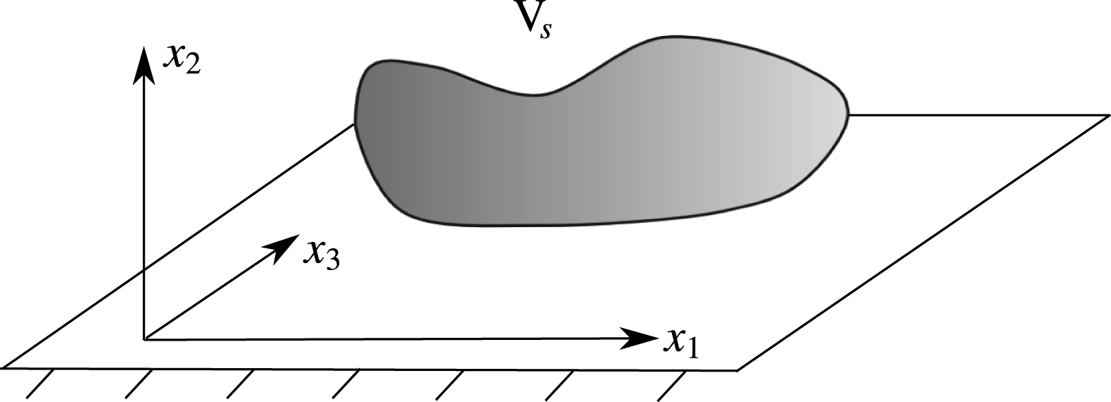
Pressure fluctuations in an incompressible turbulent boundary layer are governed by a Poisson equation. For a turbulent boundary layer along a wall located at
 $x_{2}=0$
, the Poisson equation resulting from a mean flow in the positive
 $x_{1}$
-direction becomes
 $$\begin{eqnarray}\unicode[STIX]{x0394}p=-\unicode[STIX]{x1D70C}_{0}\left(2\frac{\unicode[STIX]{x2202}U_{1}}{\unicode[STIX]{x2202}x_{2}}\frac{\unicode[STIX]{x2202}u_{2}}{\unicode[STIX]{x2202}x_{1}}+\frac{\unicode[STIX]{x2202}^{2}}{\unicode[STIX]{x2202}x_{i}\unicode[STIX]{x2202}x_{j}}(u_{i}u_{j}-\overline{u_{i}u_{j}})\right).\end{eqnarray}$$
Here,
 $U_{1}$
denotes the mean-flow velocity component in the
 $x_{1}$
-direction and
 $u_{i}$
indicates velocity fluctuations; the
 $x_{2}$
-direction is the wall normal direction and the
 $x_{3}$
-direction is the lateral direction, refer to the coordinate system shown in figure 1;
 $\unicode[STIX]{x1D70C}_{0}$
is the mean air density and
 $p$
is the fluctuating pressure. The source term on the right-hand side of (2.1) comprises two parts. The first part is the mean-shear turbulence interaction term and the second part is the turbulence–turbulence interaction term. If the boundary is a rigid flat surface, the fluctuating pressure can be calculated from the convolution of the free-space Green function of the Poisson equation with the right-hand side source term, i.e.
 $$\begin{eqnarray}p(\boldsymbol{x},t)=-\int _{\boldsymbol{V}_{\boldsymbol{s}}+\boldsymbol{V}_{\boldsymbol{s}}^{\prime }}\unicode[STIX]{x1D70C}_{0}\left(2\frac{\unicode[STIX]{x2202}U_{1}}{\unicode[STIX]{x2202}x_{2}}\frac{\unicode[STIX]{x2202}u_{2}(\boldsymbol{y},t)}{\unicode[STIX]{x2202}x_{1}}+\frac{\unicode[STIX]{x2202}^{2}}{\unicode[STIX]{x2202}x_{i}\unicode[STIX]{x2202}x_{j}}(u_{i}u_{j}-\overline{u_{i}u_{j}})(\boldsymbol{y},t)\right)\boldsymbol{\cdot }g(\boldsymbol{x}-\boldsymbol{y})\,\text{d}^{3}\boldsymbol{y}.\end{eqnarray}$$
The Green function satisfies
 $\unicode[STIX]{x1D6FB}^{2}g(\boldsymbol{x}-\boldsymbol{y})=\unicode[STIX]{x1D6FF}(\boldsymbol{x}-\boldsymbol{y})$
, where
 $\unicode[STIX]{x1D6FF}$
indicates the Dirac delta function. For the three-dimensional Poisson problem, the free-space Green function is given by
 $$\begin{eqnarray}g(\boldsymbol{x}-\boldsymbol{y})=-\frac{1}{4\unicode[STIX]{x03C0}|\boldsymbol{x}-\boldsymbol{y}|},\end{eqnarray}$$
refer to Blake (Reference Blake1986). In (2.2) the integration is carried out over the original source area
 $\boldsymbol{V}_{\boldsymbol{s}}$
plus a source area
 $\boldsymbol{V}_{\boldsymbol{s}}^{\prime }$
that represents an image of
 $\boldsymbol{V}_{\boldsymbol{s}}$
mirrored at the solid wall in order to realise the appropriate wall boundary condition
 $(\unicode[STIX]{x2202}p/\unicode[STIX]{x2202}n)_{x_{2}=0}=0$
of the pressure fluctuations (Blake Reference Blake1986).
Sketch of the coordinate system.

If we let
 $f(\boldsymbol{y},t)$
represent the source terms, the convolution integral (2.2) can be expressed as
 $$\begin{eqnarray}\int _{\boldsymbol{V}_{\boldsymbol{s}}+\boldsymbol{V}_{\boldsymbol{s}}^{\prime }}f(\boldsymbol{y},t)\boldsymbol{\cdot }g(\boldsymbol{x}-\boldsymbol{y})\,\text{d}^{3}y=(f\ast g)(\boldsymbol{x},t).\end{eqnarray}$$
Using the specific orientation of the coordinate system indicated in figure 1, the wall boundary condition becomes
 $\unicode[STIX]{x2202}p/\unicode[STIX]{x2202}x_{2}=0$
. The equation is solved in wavenumber domain by using the convolution theorem:
 $$\begin{eqnarray}{\mathcal{F}}\{\,f\ast g\}(\boldsymbol{x},t)={\mathcal{F}}\{\,f(\boldsymbol{x},t)\}\boldsymbol{\cdot }{\mathcal{F}}\{g(\boldsymbol{x})\}=\hat{f}(\boldsymbol{k},t)\boldsymbol{\cdot }{\hat{g}}(\boldsymbol{k}).\end{eqnarray}$$
Here
 $\hat{f}(\boldsymbol{k},t)={\mathcal{F}}\{\,f(\boldsymbol{x},t)\}$
denotes the three-dimensional spatial Fourier transform from the consecutive application of the one-dimensional spatial Fourier transform for all spatial coordinates
 $x_{i}$
as defined by (A 2) in the appendix A. Consequently, a solution to the Poisson problem for pressure is obtained at a given time level by multiplying the spatial Fourier transform of the time-dependent source term with the Fourier transform of the free-space Green function and subsequently transforming back the result into physical space:
 $$\begin{eqnarray}p(\boldsymbol{x},t)={\mathcal{F}}^{-1}\{\,\hat{f}(\boldsymbol{k},t)\boldsymbol{\cdot }{\hat{g}}(\boldsymbol{k})\}.\end{eqnarray}$$
As indicated above, the appropriate wall boundary condition is already realised by taking into account an image source region underneath the wall surface. However, the Fourier transform approach in general is applied on a finite computational domain and inherently realises periodicity across the domain boundaries. For an accurate numerical solution with this approach, one must assess whether the extension of the domain is large enough to ensure that despite the artificial truncation and periodicity of the Green function represented on the finite domain, it still provides a good approximation to the free-space Green function.
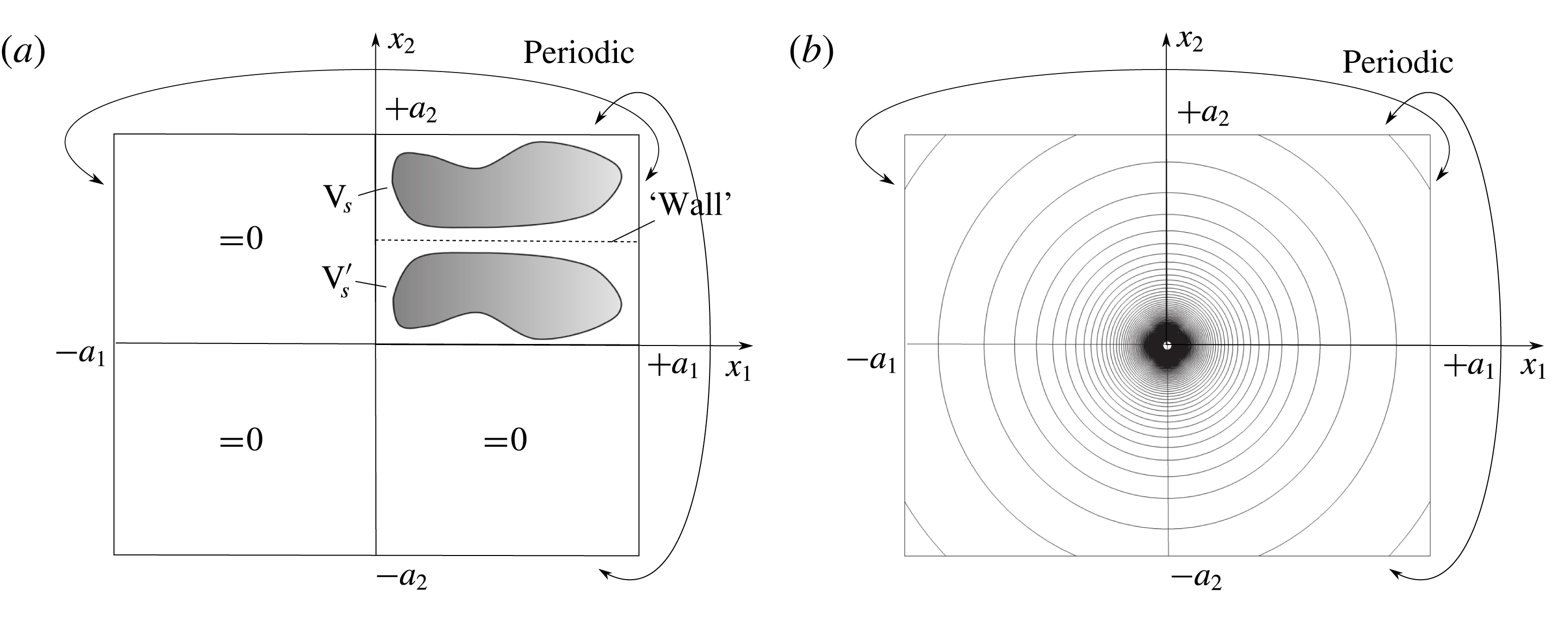
Two-dimensional sketch to illustrate application of the Hockney’s method with free field boundary condition; (a) source distribution with location of solid wall; (b) contour lines of free-space Green function (2.3).

To circumvent this problem, in this work the modification as introduced by Hockney & Eastwood (Reference Hockney and Eastwood1988) is applied, which provides an exact realisation of the free-space Green function in conjunction with a Fourier transform method on a finite domain. For Hockney’s method applied to the Poisson problem, the computational core domain can be limited to the extension of the considered right-hand side source term plus its mirror image. Then, the resulting complete computational domain follows by doubling the core domain in each spatial direction, refer to the sketch shown in figure 2(a). The Green function is prescribed on the entire domain. A source distribution for the complete domain is obtained by zero padding of the source in the appended domains. Hence, the source function and the Green function for the resolved domain become
 $$\begin{eqnarray}\displaystyle & \displaystyle f(\boldsymbol{x})=\left\{\begin{array}{@{}ll@{}}f(\boldsymbol{x}),\quad & 0\leqslant x_{i}\leqslant a_{i};i\in \{1\ldots 3\},\\ 0,\quad & \text{else}.\end{array}\right. & \displaystyle\end{eqnarray}$$
 $$\begin{eqnarray}\displaystyle & \displaystyle g(\boldsymbol{x})=-\frac{1}{4\unicode[STIX]{x03C0}|\boldsymbol{x}|},\quad -a_{i}\leqslant x_{i}\leqslant a_{i};i\in \{1\ldots 3\}. & \displaystyle\end{eqnarray}$$
To sketch the basic idea behind Hockney’s approach, it is convenient to consider the underlying spatial convolution (2.4). If we seek for a solution to the Poisson problem just in a core source domain of spatial extensions
 $a_{i}$
, the convolution integral includes products of the source term with the free-space Green function evaluated at a shifted position, which involve at maximum a shift in each direction given by
 $a_{i}$
. Hence, if a Green function with periodic continuation is applied that is specified over twice the width of the core source distribution, i.e.
 $2a_{i}$
, figure 2(b), and no further source contribution is considered in the extended domain (zero padding), figure 2(a), the convolution integral will provide inside the core domain an exact solution to the Poisson problem based on the free-space Green function.
2.2 Fast random particle–mesh method
2.2.1 Anisotropic synthetic turbulence
To calculate the fluctuating pressure an appropriate fluctuating velocity field within the turbulent boundary layer is needed. We use the fast random particle–mesh method (FRPM) (Ewert et al.
Reference Ewert, Dierke, Siebert, Neifeld, Appel, Siefert and Kornow2011) to generate synthetic turbulent velocity fluctuations to prescribe the right-hand side source term of (2.1). FRPM uses averaged turbulence statistics to synthesise the turbulent velocity fluctuations. One- and two-point statistics are realised. The basic idea is to generate a fluctuating velocity vector from the convolution of spatial white noise
 ${\mathcal{U}}_{i}$
with a spatial Gaussian filter kernel
 $G$
,
 $$\begin{eqnarray}u_{i}(\boldsymbol{x},t)=\hat{\unicode[STIX]{x1D622}}_{ik}(\boldsymbol{x})\int _{V_{s}}\unicode[STIX]{x1D716}_{klm}\frac{\unicode[STIX]{x2202}G(\boldsymbol{x}-\boldsymbol{x}^{\prime })}{\unicode[STIX]{x2202}x_{l}}{\mathcal{U}}_{m}(\boldsymbol{x}^{\prime },t)\,\text{d}^{3}\boldsymbol{x}^{\prime },\end{eqnarray}$$
where
 $\unicode[STIX]{x1D716}_{klm}$
denotes the Levi-Civita symbol (permutation tensor),
 $\boldsymbol{x}=(x_{1},x_{2},x_{3})^{\text{T}}$
defines field coordinates and
 $\boldsymbol{x}^{\prime }=(x_{1}^{\prime },x_{2}^{\prime },x_{3}^{\prime })^{\text{T}}$
defines white noise field coordinates. The Gaussian filter is defined by the consecutive application of one-dimensional (1-D) Gaussian filters based on separate length scales
 $l_{i}$
for each spatial direction,
 $$\begin{eqnarray}G(\boldsymbol{x}-\boldsymbol{x}^{\prime })=g(x_{1}-x_{1}^{\prime },l_{1})\,g(x_{2}-x_{2}^{\prime },l_{2})\,g(x_{3}-x_{3}^{\prime },l_{3}),\end{eqnarray}$$
with
 $$\begin{eqnarray}g(y,l):=\exp \left(-\frac{\unicode[STIX]{x03C0}}{2}\frac{y^{2}}{l^{2}}\right).\end{eqnarray}$$
The tensor
 $\hat{\unicode[STIX]{x1D622}}_{ik}$
provides the proper scaling so that the anisotropic Reynolds stress tensor can be realised by the synthesised fluctuating velocity fields. Note, the summation rule is applied over all equal indices.
In this work a generic study is conducted on the influence of length scale anisotropy on the resulting wall pressure spectrum. For this purpose, anisotropy in length scales is considered using separate filter length scales
 $l_{i}$
in the streamwise, wall-normal and spanwise directions, respectively. Furthermore, the streamwise length scale is increased by a stretching factor
 $\unicode[STIX]{x1D6FE}$
compared to the wall-normal scale,
 $l_{1}=\unicode[STIX]{x1D6FE}l_{2}$
, whereas the length scales in the wall-normal and spanwise directions are kept equal,
 $l_{2}=l_{3}$
. For the present study, the stretching factor is treated as a constant parameter throughout the computational domain. Note, in general three spatial length scales are associated with each Reynolds stress component, yielding a third-rank tensor with 18 generally non-equal components. This anisotropic length scale information is not provided by Reynolds-averaged Navier–Stokes (RANS) equations. In Ewert (Reference Ewert2016) an approach to stochastically model anisotropic length scales from RANS parameters for non-equilibrium turbulence has been proposed.
In general, the length scale from RANS
 $l_{s}$
is considered as a scalar scale representing all anisotropic scales (Wilcox Reference Wilcox2006) assuming the relationship
 $l_{s}=(l_{1}l_{2}l_{3})^{1/3}$
, which yields
 $l_{2}=l_{3}=l_{s}\unicode[STIX]{x1D6FE}^{-1/3}$
.
The scalar turbulent length scale
 $l_{s}$
is determined from the RANS solution via
 $$\begin{eqnarray}l_{s}=\frac{c_{l}}{C_{\unicode[STIX]{x1D707}}}\frac{\sqrt{k_{t}}}{\unicode[STIX]{x1D714}},\end{eqnarray}$$
where
 $k_{t}=\unicode[STIX]{x1D619}_{ii}/2$
is the turbulent kinetic energy and
 $\unicode[STIX]{x1D714}$
is the specific rate of dissipation. The constant
 $C_{\unicode[STIX]{x1D707}}=0.09$
and
 $c_{l}$
is estimated to be 0.54 (Bailly & Juvé Reference Bailly and Juvé1999), so the prefactor
 $c_{l}/C_{\unicode[STIX]{x1D707}}\simeq 6.0$
.
The white noise field
 ${\mathcal{U}}_{i}$
is defined in a Lagrangian frame moving at local flow velocity
 $\boldsymbol{U}$
. Altogether, the properties of white noise are defined in a fixed Eulerian frame by
 $$\begin{eqnarray}\displaystyle & \displaystyle \langle {\mathcal{U}}_{i}(\boldsymbol{x}^{\prime },t)\rangle =0, & \displaystyle\end{eqnarray}$$
 $$\begin{eqnarray}\displaystyle & \displaystyle \langle {\mathcal{U}}_{i}(\boldsymbol{x}^{\prime },t){\mathcal{U}}_{j}(\boldsymbol{x}^{\prime }+\boldsymbol{r},t+\unicode[STIX]{x1D70F})\rangle =\unicode[STIX]{x1D6FF}(\boldsymbol{r}-\boldsymbol{U}\unicode[STIX]{x1D70F})\unicode[STIX]{x1D6FF}_{ij}, & \displaystyle\end{eqnarray}$$
where the bracket means an ensemble average,
 $\unicode[STIX]{x1D6FF}_{ij}$
is the Kronecker symbol and
 $\unicode[STIX]{x1D6FF}(\boldsymbol{r}-\boldsymbol{U}\unicode[STIX]{x1D70F})$
describes a frozen turbulence flow moving with the flow velocity
 $\boldsymbol{U}$
. Additional temporal turbulence decay can be modelled by a Langevin equation, which introduces the decorrelation in the two-point statistics (Ewert et al.
Reference Ewert, Dierke, Siebert, Neifeld, Appel, Siefert and Kornow2011). In the Eulerian frame a modification of the cross-correlation is given by
 $$\begin{eqnarray}\langle {\mathcal{U}}_{i}(\boldsymbol{x}^{\prime },t){\mathcal{U}}_{j}(\boldsymbol{x}^{\prime }+\boldsymbol{r},t+\unicode[STIX]{x1D70F})\rangle =\unicode[STIX]{x1D6FF}(\boldsymbol{r}-\boldsymbol{U}\unicode[STIX]{x1D70F})\exp \left(-\frac{|\unicode[STIX]{x1D70F}|}{\unicode[STIX]{x1D70F}_{s}}\right)\unicode[STIX]{x1D6FF}_{ij}.\end{eqnarray}$$
In this expression
 $\exp (-|\unicode[STIX]{x1D70F}|/\unicode[STIX]{x1D70F}_{s})$
describes the turbulence decay, i.e. the field is spatially white and correlated in time with time scale
 $\unicode[STIX]{x1D70F}_{s}$
. The local time scale can be determined from RANS solutions by
 $$\begin{eqnarray}\unicode[STIX]{x1D70F}_{s}=c_{\unicode[STIX]{x1D70F}}\frac{l_{s}}{\sqrt{k_{t}}},\end{eqnarray}$$
where the prefactor
 $c_{\unicode[STIX]{x1D70F}}$
needs to be determined. Tam & Auriault (Reference Tam and Auriault1999) modelled the time scale in a
 $k-\unicode[STIX]{x1D716}$
model and determined the prefactor empirically by fitting experimental results of jet flows, which resulted in
 $c_{\unicode[STIX]{x1D70F}}\simeq 0.91$
. In this work, a constant
 $c_{\unicode[STIX]{x1D70F}}=1.2$
is applied which is based on a consistent result of the longitudinal coherence of the wall pressure fluctuations compared to the experimental results. The additional effect of the temporal turbulence decay for turbulence velocity fluctuation spectra is discussed in appendix A.
2.2.2 Scaling tensor
For a stationary turbulent problem, straightforward manipulation of expression (2.9) yields the Reynolds stresses expressed in terms of the scaling tensor,
 $$\begin{eqnarray}\displaystyle \unicode[STIX]{x1D619}_{ij}(\boldsymbol{x})=\langle u_{i}(\boldsymbol{x},t)u_{j}(\boldsymbol{x},t)\rangle & = & \displaystyle \hat{\unicode[STIX]{x1D622}}_{ik}(\boldsymbol{x})\hat{\unicode[STIX]{x1D622}}_{jn}(\boldsymbol{x})\int _{V_{s}}\unicode[STIX]{x1D716}_{klm}\unicode[STIX]{x1D716}_{nop}\frac{\unicode[STIX]{x2202}G(\boldsymbol{x}-\boldsymbol{x}^{\prime })}{\unicode[STIX]{x2202}x_{l}}\frac{\unicode[STIX]{x2202}G(\boldsymbol{x}-\boldsymbol{x}^{\prime \prime })}{\unicode[STIX]{x2202}x_{o}}\nonumber\\ \displaystyle & & \displaystyle \times \,\langle {\mathcal{U}}_{m}(\boldsymbol{x}^{\prime },t){\mathcal{U}}_{p}(\boldsymbol{x}^{\prime \prime },t)\rangle \,\text{d}^{3}\boldsymbol{x}^{\prime }\,\text{d}^{3}\boldsymbol{x}^{\prime \prime }.\end{eqnarray}$$
Based on (2.15) with
 $\unicode[STIX]{x1D70F}=0$
and
 $\boldsymbol{r}=0$
, the integration over the delta function related to
 $\boldsymbol{x}^{\prime \prime }$
can be carried out. Using the definition
 $$\begin{eqnarray}{\mathcal{I}}_{ij}(\boldsymbol{x}):=\int _{V_{s}}\frac{\unicode[STIX]{x2202}G(\boldsymbol{x}-\boldsymbol{x}^{\prime })}{\unicode[STIX]{x2202}x_{i}}\frac{\unicode[STIX]{x2202}G(\boldsymbol{x}-\boldsymbol{x}^{\prime })}{\unicode[STIX]{x2202}x_{j}}\,\text{d}^{3}\boldsymbol{x}^{\prime },\end{eqnarray}$$
the Reynolds stresses eventually read (dependence on spatial coordinate not explicitly shown)
 $$\begin{eqnarray}\unicode[STIX]{x1D619}_{ij}=\hat{\unicode[STIX]{x1D622}}_{ik}\hat{\unicode[STIX]{x1D622}}_{jn}\unicode[STIX]{x1D716}_{mlk}\unicode[STIX]{x1D716}_{mon}{\mathcal{I}}_{lo}.\end{eqnarray}$$
Furthermore, using the identity
 $\unicode[STIX]{x1D716}_{mlk}\unicode[STIX]{x1D716}_{mon}=\unicode[STIX]{x1D6FF}_{lo}\unicode[STIX]{x1D6FF}_{kn}-\unicode[STIX]{x1D6FF}_{ln}\unicode[STIX]{x1D6FF}_{ko}$
, it follows
 $$\begin{eqnarray}\unicode[STIX]{x1D619}_{ij}=\hat{\unicode[STIX]{x1D622}}_{ik}\hat{\unicode[STIX]{x1D622}}_{jl}\unicode[STIX]{x1D61A}_{kl},\end{eqnarray}$$
where
 $\unicode[STIX]{x1D61A}_{kl}=\unicode[STIX]{x1D6FF}_{kl}{\mathcal{I}}_{mm}-{\mathcal{I}}_{lk}$
defines a symmetric diagonal matrix, since
 ${\mathcal{I}}_{lk}=0$
for
 $l\neq k$
as a result of its definition (2.18) with filter function (2.10). Let
 $\unicode[STIX]{x1D634}_{km}=c_{(k)}\unicode[STIX]{x1D6FF}_{km}$
(the brackets indicate omission of the summation rule) denote the diagonal matrix that follows by taking the square root of the diagonal elements of
 $\unicode[STIX]{x1D61A}_{kl}=c_{(k)}c_{(l)}\unicode[STIX]{x1D6FF}_{kl}$
(i.e.
 $\unicode[STIX]{x1D61A}_{kl}=\unicode[STIX]{x1D634}_{km}\unicode[STIX]{x1D634}_{lm}$
) and let
 $r_{ij}$
denote the Cholesky decomposition of the Reynolds stress tensor, i.e.
 $\unicode[STIX]{x1D619}_{ij}=\unicode[STIX]{x1D633}_{im}\unicode[STIX]{x1D633}_{jm}$
, then the scaling tensor needed to evaluate (2.9) is defined by
 $\unicode[STIX]{x1D633}_{im}=\hat{\unicode[STIX]{x1D622}}_{ik}\unicode[STIX]{x1D634}_{km}$
, respectively,
 $$\begin{eqnarray}\hat{\unicode[STIX]{x1D622}}_{ik}=\unicode[STIX]{x1D633}_{ik}/c_{(k)}.\end{eqnarray}$$
From the previous discussion it follows that the scaling explicitly is defined by
 $c_{(k)}=\sqrt{{\mathcal{I}}_{ll}-{\mathcal{I}}_{k(k)}}$
.
Using the definition of the integral equation (2.18) together with the length scale definitions from the beginning of this section and applying the definition of the Gaussian filter, equation (2.10), the scaling parameters
 $c_{(k)}$
can be explicitly evaluated, yielding
 $$\begin{eqnarray}c_{(1)}=\sqrt{\unicode[STIX]{x03C0}l_{s}}\unicode[STIX]{x1D6FE}^{1/3},\quad c_{(2)}=\sqrt{\frac{\unicode[STIX]{x03C0}l_{s}}{2}}\frac{\sqrt{1+\unicode[STIX]{x1D6FE}^{2}}}{\unicode[STIX]{x1D6FE}^{2/3}},\quad c_{(3)}=\sqrt{\frac{\unicode[STIX]{x03C0}l_{s}}{2}}\frac{\sqrt{1+\unicode[STIX]{x1D6FE}^{2}}}{\unicode[STIX]{x1D6FE}^{2/3}}.\end{eqnarray}$$
Next, the Cholesky decomposition of the in general anisotropic Reynolds stress tensor
 $\unicode[STIX]{x1D619}_{ij}$
from RANS with a Reynolds stress model is deduced from
 $$\begin{eqnarray}(\unicode[STIX]{x1D633}_{ij})=\left(\begin{array}{@{}ccc@{}}\sqrt{\unicode[STIX]{x1D619}_{11}}\quad & 0\quad & 0\\ \unicode[STIX]{x1D619}_{21}/\unicode[STIX]{x1D633}_{11}\quad & \sqrt{\unicode[STIX]{x1D619}_{22}-\unicode[STIX]{x1D633}_{21}^{2}}\quad & 0\\ \unicode[STIX]{x1D619}_{31}/\unicode[STIX]{x1D633}_{11}\quad & (\unicode[STIX]{x1D619}_{32}-\unicode[STIX]{x1D633}_{21}\unicode[STIX]{x1D633}_{31})/\unicode[STIX]{x1D633}_{22}\quad & \sqrt{\unicode[STIX]{x1D619}_{33}-\unicode[STIX]{x1D633}_{31}^{2}-\unicode[STIX]{x1D633}_{32}^{2}}\end{array}\right),\end{eqnarray}$$
which can be solved starting with the first row and using successively for the evaluation of the consecutive rows already computed components of
 $\unicode[STIX]{x1D633}_{ij}$
.
According to this procedure, the tensor
 $\unicode[STIX]{x1D61A}_{kl}$
can be Cholesky decomposed into the matrix
 $\unicode[STIX]{x1D634}_{km}$
and the final scaling matrix follows by multiplying
 $\unicode[STIX]{x1D633}_{im}$
with the inverse of
 $\unicode[STIX]{x1D634}_{km}$
,
 $\hat{\unicode[STIX]{x1D622}}_{ik}=\unicode[STIX]{x1D633}_{im}\unicode[STIX]{x1D634}_{km}^{-1}$
. The properties as defined by (2.18) guarantee that
 $\unicode[STIX]{x1D61A}_{kl}$
is diagonal and can be used to derive the scaling
 $c_{(k)}$
by taking the square root and the inverse of the diagonal elements, which essentially represents the Cholesky decomposition of
 $\unicode[STIX]{x1D61A}_{kl}$
and leads to scaling equation (2.21).
Eventually, the final anisotropic simulation is conducted by using the such determined scaling matrix
 $\hat{\unicode[STIX]{x1D622}}_{ik}$
.
2.2.3 Isotropic turbulence
For isotropic turbulence the following relationships hold:
 $\hat{\unicode[STIX]{x1D622}}_{ik}(\boldsymbol{x})\rightarrow \hat{a}(\boldsymbol{x})\unicode[STIX]{x1D6FF}_{ik}$
,
 $\unicode[STIX]{x1D6FE}=1$
(i.e.
 $l_{1}=l_{2}=l_{3}=l_{s}$
),
 $\unicode[STIX]{x1D619}_{11}=\unicode[STIX]{x1D619}_{22}=\unicode[STIX]{x1D619}_{33}=2/3k_{t}$
, and
 $\unicode[STIX]{x1D619}_{ij}=0$
for
 $i\neq j$
. Consequently, from (2.21) the scalar scaling function for isotropic turbulence infers
 $$\begin{eqnarray}\hat{a}(\boldsymbol{x})=\sqrt{\frac{2}{3\unicode[STIX]{x03C0}}\frac{k_{t}(\boldsymbol{x})}{l_{s}(\boldsymbol{x})}}.\end{eqnarray}$$
Furthermore, for homogeneous isotropic turbulence
 $\hat{a}=\text{const.}$
and integral equation (2.9) can be rewritten as
 $$\begin{eqnarray}\boldsymbol{u}=\unicode[STIX]{x1D735}\times \unicode[STIX]{x1D753},\end{eqnarray}$$
with
 $\unicode[STIX]{x1D753}=(\unicode[STIX]{x1D719}_{1},\unicode[STIX]{x1D719}_{2},\unicode[STIX]{x1D719}_{3})^{\text{T}}$
and
 $$\begin{eqnarray}\unicode[STIX]{x1D719}_{i}:=\int _{V_{s}}\hat{a}\,G{\mathcal{U}}_{i}\,\text{d}^{3}\boldsymbol{x}^{\prime }.\end{eqnarray}$$
The two-point correlations of the velocity fluctuations realise the normalised correlation tensor of homogeneous isotropic turbulence
 $\hat{\unicode[STIX]{x1D619}}_{ij}(r)$
for two points
 $\boldsymbol{x}_{i}$
and
 $\boldsymbol{x}_{j}$
with distance
 $r=|\boldsymbol{x}_{i}-\boldsymbol{x}_{j}|$
and the expected relationship between longitudinal and lateral correlation functions
 $f(r)$
and
 $g(r)$
, respectively (Batchelor Reference Batchelor1982),
 $$\begin{eqnarray}\displaystyle & \displaystyle \hat{\unicode[STIX]{x1D619}}_{ij}=(f(r)-g(r))\frac{r_{i}r_{j}}{r^{2}}+g(r)\unicode[STIX]{x1D6FF}_{ij}, & \displaystyle\end{eqnarray}$$
 $$\begin{eqnarray}\displaystyle & \displaystyle g(r)=f(r)+\frac{r}{2}\frac{\text{d}f(r)}{\text{d}r}. & \displaystyle\end{eqnarray}$$
For a Gaussian filter kernel defined by (2.10), the resulting longitudinal correlation function for homogeneous isotropic turbulence is also a Gaussian (Ewert Reference Ewert2008) defined by
 $$\begin{eqnarray}f(r)=\exp \left(-\frac{\unicode[STIX]{x03C0}r^{2}}{4l_{s}^{2}}\right).\end{eqnarray}$$
Based on the specific scaling of the Gaussian filter function (2.10), which leads to the longitudinal correlation (2.29), the length scale used therein complies with the integral length scale
 $L$
derived from the longitudinal function,
 $$\begin{eqnarray}L:=\int _{0}^{\infty }f(r)\,\text{d}r=l_{s}.\end{eqnarray}$$
The length scale related to the lateral correlation function obeys
 $$\begin{eqnarray}\int _{0}^{\infty }g(r)\,\text{d}r=\frac{l_{s}}{2}.\end{eqnarray}$$
2.2.4 Numerical realisation
For the quadrature of the integral in (2.9) the computational domain is formally split into equal sized non-overlapping control volumes
 $\unicode[STIX]{x1D6FF}V_{p}$
of constant size, continuously covering the resolved source domain without holes. A random particle is assigned to the centre of each control volume
 $\boldsymbol{x}_{p}$
. All resulting particles are moving with their local convection velocity at the particle location. The control volumes are bounded by liquid-line surfaces, i.e. the boundary surface is drifting with the flow and in incompressible flow the control volume
 $\unicode[STIX]{x1D6FF}V_{p}$
is invariant over time. The extension of the procedure to compressible flow was discussed in Ewert et al. (Reference Ewert, Dierke, Siebert, Neifeld, Appel, Siefert and Kornow2011). Random variables are attached to each particle. Their random variates at time level
 $t^{n+1}$
formally are defined by the integral over the control volume of the stochastic fields at the current time level, i.e.
 $$\begin{eqnarray}r_{ip}^{n+1}:=\int _{\unicode[STIX]{x1D6FF}V_{p}}{\mathcal{U}}_{i}(\boldsymbol{x}^{\prime },t^{n+1})\,\text{d}^{3}\boldsymbol{x}^{\prime }.\end{eqnarray}$$
The notion ‘random variate’ is used here to indicate the specific value of a random variable at a specific time level, e.g. random variates
 $r_{ip}^{n+1}$
indicate the value of random variables
 $r_{ip}$
at time level
 $n+1$
. Eventually, the convolution equation (2.9) is approximated at discrete time level
 $n+1$
by summation over all control volumes,
 $$\begin{eqnarray}u_{i}^{n+1}(\boldsymbol{x})\simeq \mathop{\sum }_{p}\hat{\unicode[STIX]{x1D622}}_{ik}\unicode[STIX]{x1D716}_{klm}\frac{\unicode[STIX]{x2202}}{\unicode[STIX]{x2202}x_{l}}G(\boldsymbol{x}-\boldsymbol{x}_{p})r_{mp}^{n+1}.\end{eqnarray}$$
Numerically, only random variables
 $r_{mp}$
are realised and the stochastic field
 ${\mathcal{U}}_{i}$
serves only to facilitate the derivation of a discretised random process to generate the actual variates of each random variable.
The numerical procedure to realise the simulation steps as discussed before relies on an additional block structured mesh that defines the domain where synthetic turbulence is generated, hereafter denoted as ‘FRPM domain’. In this work a Cartesian equidistant mesh is used. However, also general curvilinear meshes could be used. The mean flow as well as the local amplitude scaling function of the fluctuations, equation (2.24), and the local length and time scales, equations (2.12) and (2.16), respectively, are evaluated from the RANS solution and interpolated onto the FRPM mesh.
For frozen turbulence, the random value carried by each particle is constant over time. Hence, its value is generated when a random particle is entering the computational domain and kept constant while the particle is convected through the computational domain. When a random particle is leaving the computational domain it is reseeded with an updated random value at the upstream boundary so that the number of particles remains invariant and the mean particle density is conserved.
For decaying turbulence a discretised Langevin equation is solved for each random variate, refer to Ewert et al. (Reference Ewert, Dierke, Siebert, Neifeld, Appel, Siefert and Kornow2011), whose discretised form reads Pope (Reference Pope2000)
 $$\begin{eqnarray}r_{ip}^{n+1}=\left(1-\frac{\unicode[STIX]{x0394}t}{\unicode[STIX]{x1D70F}_{s}}\right)r_{ip}^{n}+\left(\frac{2\unicode[STIX]{x1D6FF}V_{p}\unicode[STIX]{x0394}t}{\unicode[STIX]{x1D70F}_{s}}\right)^{1/2}\unicode[STIX]{x1D70E}_{ip}^{n},\end{eqnarray}$$
where
 $\unicode[STIX]{x1D70E}_{ip}^{n}$
are mutually uncorrelated standardised Gaussian random variates, which are independent of themselves at different times (
 $\langle \unicode[STIX]{x1D70E}_{ip}^{n}\rangle =0$
,
 $\langle \unicode[STIX]{x1D70E}_{ip}^{n}\unicode[STIX]{x1D70E}_{jq}^{m}\rangle =\unicode[STIX]{x1D6FF}_{ij}\unicode[STIX]{x1D6FF}_{pq}\unicode[STIX]{x1D6FF}_{nm}$
) and which are independent of
 $r_{ip}^{m}$
at past times (e.g.
 $\langle \unicode[STIX]{x1D70E}_{ip}^{n}r_{jq}^{m}\rangle =0$
for
 $t^{m}\leqslant t^{n}$
). The time increment between time levels
 $t^{n+1}$
and
 $t^{n}$
is given by
 $\unicode[STIX]{x0394}t<\unicode[STIX]{x1D70F}_{s}$
. Furthermore,
 $\unicode[STIX]{x1D6FF}V_{p}$
indicates the control volume associated with each particle according to (2.32).
For frozen turbulence (
 $\unicode[STIX]{x1D70F}_{s}\rightarrow \infty$
), from the previous procedure it follows that
 $r_{ip}^{n+1}=r_{ip}^{n}$
, i.e. the random variate is invariant over time. For frozen turbulence, the initial variance of the random variate associated with each particle scales with
 $\unicode[STIX]{x1D6FF}V_{p}$
, i.e. the inverse local particle density.
Mean flow and other quantities needed at a specific particle position are obtained similar to particle-in-cell (PIC) methods by trilinear mapping of the mean-flow information stored on the FRPM patch mesh from the corners of a specific hosting cell to the actual particle position inside the cell.
The complete algorithm to generated a fluctuating velocity field at time level
 $n+1$
can be summarised as follows:
-
(i) based on the mean-flow velocity at the particle position, move the particles from old position at time level
 $n$
to the new one at time level
$n+1$
;
-
(ii) realise with (2.34) new variates of all random variables attached to each particle;
-
(iii) distribute random variates via discretised convolution equation (2.33) onto the source domain;
-
(iv) evaluate the right-hand side source term of the Poisson equation (2.1) and solve it via Hockney’s method to predict the wall pressure at time level
$n+1$
.


The discretised convolution consists of a projection step, where the random variates are mapped from the actual particle position to the surrounding hosting cell nodes and the spatial filter steps are pursued sequentially on the FRPM mesh along each coordinate direction using direction-dependent filter length scales
 $l_{i}$
.
In order to avoid a particle convecting no further away than into a cell attached to the actual hosting cell, the maximum time step is limited by a Courant–Friedrichs–Lewy (CFL)-like condition based on the mesh spacing and the local mean-flow convection velocity.
A discussion of the methods applied for the seeding of particles at inflow boundaries (and removal at outflow boundaries) and the efficient realisation of the discrete convolution via recursive Gaussian filters can be found in Siefert & Ewert (Reference Siefert and Ewert2009) and Ewert et al. (Reference Ewert, Dierke, Siebert, Neifeld, Appel, Siefert and Kornow2011).
3 Computational set-up and flow parameters
Mean-flow statistics for two-dimensional flows over a flat plate are gained from RANS solutions. Two velocities related to Mach numbers
 $Ma=0.1$
and
 $Ma=0.2$
are calculated using German Aerospace Center (DLR)’s in-house computational fluid dynamics (CFD) solver TAU. The Reynolds stress model with specific dissipation (
 $\unicode[STIX]{x1D714}$
) equation is used for the computation. A structured grid with approximately 200 k mesh points is used and the boundary layer is solved with the first cell layer
 $y^{+}<1$
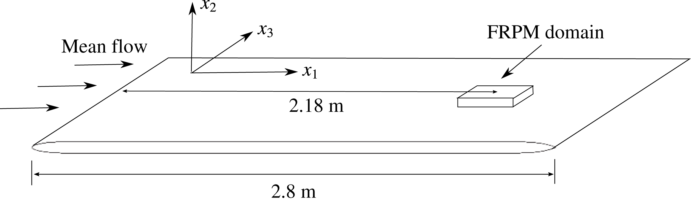
. The geometry of the computational domain is sketched in figure 3. The length of the whole plate is 2.8 m with an elliptical leading edge and a parabolic-shaped trailing edge. The leading edge and trailing edge sections have a length of 18 cm and 22 cm, respectively. The thickness of the plate is 6 cm.
Sketch of the computational domain.

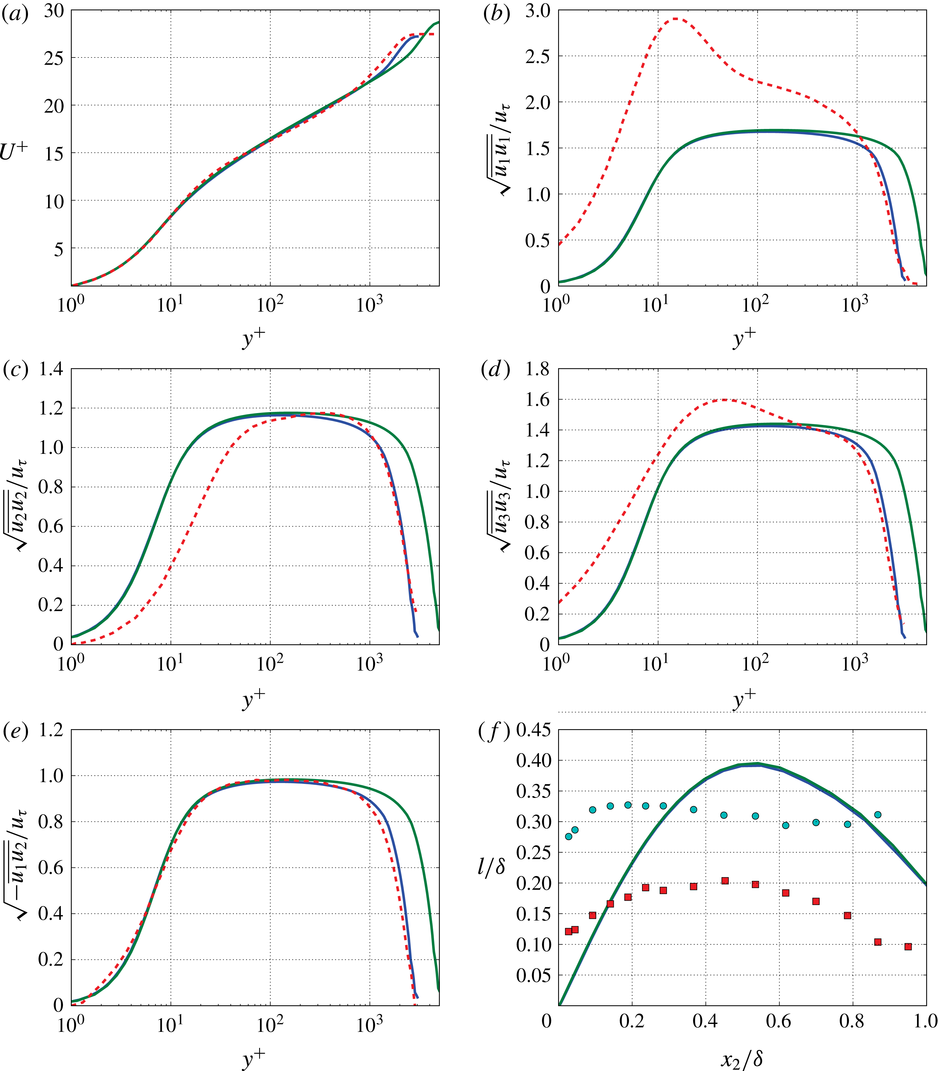
Boundary layer parameters at
 $x_{1}=2.18$
m along direction normal to the wall; (——), RANS solutions with
 $Ma=0.1$
at
 $\mathit{Re}_{\unicode[STIX]{x1D703}}=8257$
and
 $Ma=0.2$
at
 $\mathit{Re}_{\unicode[STIX]{x1D703}}=14\,668$
; (– – –), LES results from Eitel-Amor, Örlü & Schlatter (Reference Eitel-Amor, Örlü and Schlatter2014) at
 $\mathit{Re}_{\unicode[STIX]{x1D703}}=7500$
; ●, ▪, measured length scale and modified length scale for an isotropic turbulence approach from Kamruzzaman et al. (Reference Kamruzzaman, Lutz, Herrig and Krämer2012) at
 $\mathit{Re}_{\unicode[STIX]{x1D703}}=5363$
. (a) Mean flow profile; (b–e) root mean squared Reynolds stress tensors; (f) length scale from (2.12).

Synthetic turbulence is realised by FRPM for a three-dimensional rectangular domain with its centre located 2.18 m downstream of the leading edge, see figure 3. The extension of the FRPM computational domain in streamwise, wall-normal and spanwise directions, respectively, are
 $L_{1}=7\unicode[STIX]{x1D6FF}$
,
 $L_{2}=1.2\unicode[STIX]{x1D6FF}$
and
 $L_{3}=4\unicode[STIX]{x1D6FF}$
, where
 $\unicode[STIX]{x1D6FF}$
denotes the boundary layer thickness at the centre of the domain. Since Hockney’s method demands a grid with
 $2^{N}$
mesh points in each direction, a Cartesian grid with
 $128\times 64\times 128$
points is chosen for the calculations. A smaller time step is needed for the
 $Ma=0.2$
case due to the ‘CFL’-like constraint of FRPM, refer to § 2.2. Therefore, two time steps i.e.
 $\unicode[STIX]{x0394}t=4.37\times 10^{-5}$
and
 $\unicode[STIX]{x0394}t=2\times 10^{-5}$
are used, the smaller one for the
 $Ma=0.2$
case and the
 $Ma=0.1$
case with detailed two-point statistics analysis, the larger one for other
 $Ma=0.1$
cases. The calculations are run on a desktop computer with Inter Xeon E5-2630 2.4 GHz central processing units (CPUs). Each calculation for the pressure fluctuations is computed with 4 CPUs (8 threads) and the calculation time for 1 s with the coarser time step is approximately 450 CPU hours and approximately 1000 h for the case with the smaller time step. For the present simulations, a detailed two-point statistics analysis is conducted for the
 $Ma=0.1$
case and 2 s real time; all other cases utilise 1 s simulation time samples.
Turbulent boundary layer parameters.

The characteristics of the turbulent boundary layer at the centre position of the domain (
 $x_{1}=2.18$
m) are listed in table 1. The obtained boundary layer shape factors
 $H=1.34$
for
 $\mathit{Re}_{\unicode[STIX]{x1D703}}=8257$
and
 $H=1.31$
for
 $\mathit{Re}_{\unicode[STIX]{x1D703}}=14\,668$
show very good agreement (
 $\pm 1\,\%$
) with the prediction from Chauhan, Monkewitz & Nagib (Reference Chauhan, Monkewitz and Nagib2009). The mean velocity profiles show good agreement with the LES result from Eitel-Amor et al. (Reference Eitel-Amor, Örlü and Schlatter2014) at a comparable Reynolds number, see figure 4(a). Figure 4(b–e) shows comparison of the Reynolds stress between RANS solutions and the numerical data sets. The RANS results underpredict the Reynolds stress tensor
 $\overline{u_{1}u_{1}}$
in the sublayer and the logarithmic region compared to the LES results. The Reynolds stress tensor components
 $\overline{u_{2}u_{2}}$
and
 $\overline{u_{3}u_{3}}$
show good agreement with the LES results, except for some discrepancies in the region very close to the wall. For a two-dimensional boundary layer, the Reynolds stress tensors
 $\overline{u_{1}u_{3}}$
and
 $\overline{u_{2}u_{3}}$
are equal to zero (Pope Reference Pope2000). The length scale predicted by (2.12) as an averaged isotropic length scale is compared to the experimental results from Kamruzzaman et al. (Reference Kamruzzaman, Lutz, Herrig and Krämer2012) in figure 4(f). The smaller value is the measured length scale for
 $u_{2}$
and was measured at 1 % chord length downstream of the trailing edge of a NACA 0012 airfoil at
 $0^{\circ }$
angle of attack. The larger one is the modified length scale obtained by using an isotropic turbulence approach to fit the measured velocity fluctuation spectra. The length scale from RANS solutions fit the modified length scale better in the outer layer and the measured one in the inner layer.
4 Results
4.1 Turbulence velocity fluctuations realisation
Turbulent velocity fluctuations realised by FRPM are used to prescribe the fluctuating source terms of the Poisson equation (2.1) to derive unsteady wall pressure fluctuations. In a first step, isotropic fluctuations are realised by using a constant (isotropic) length scale in the spatial filter function (2.10) for each direction, i.e.
 $l_{1}=l_{2}=l_{3}=l_{s}$
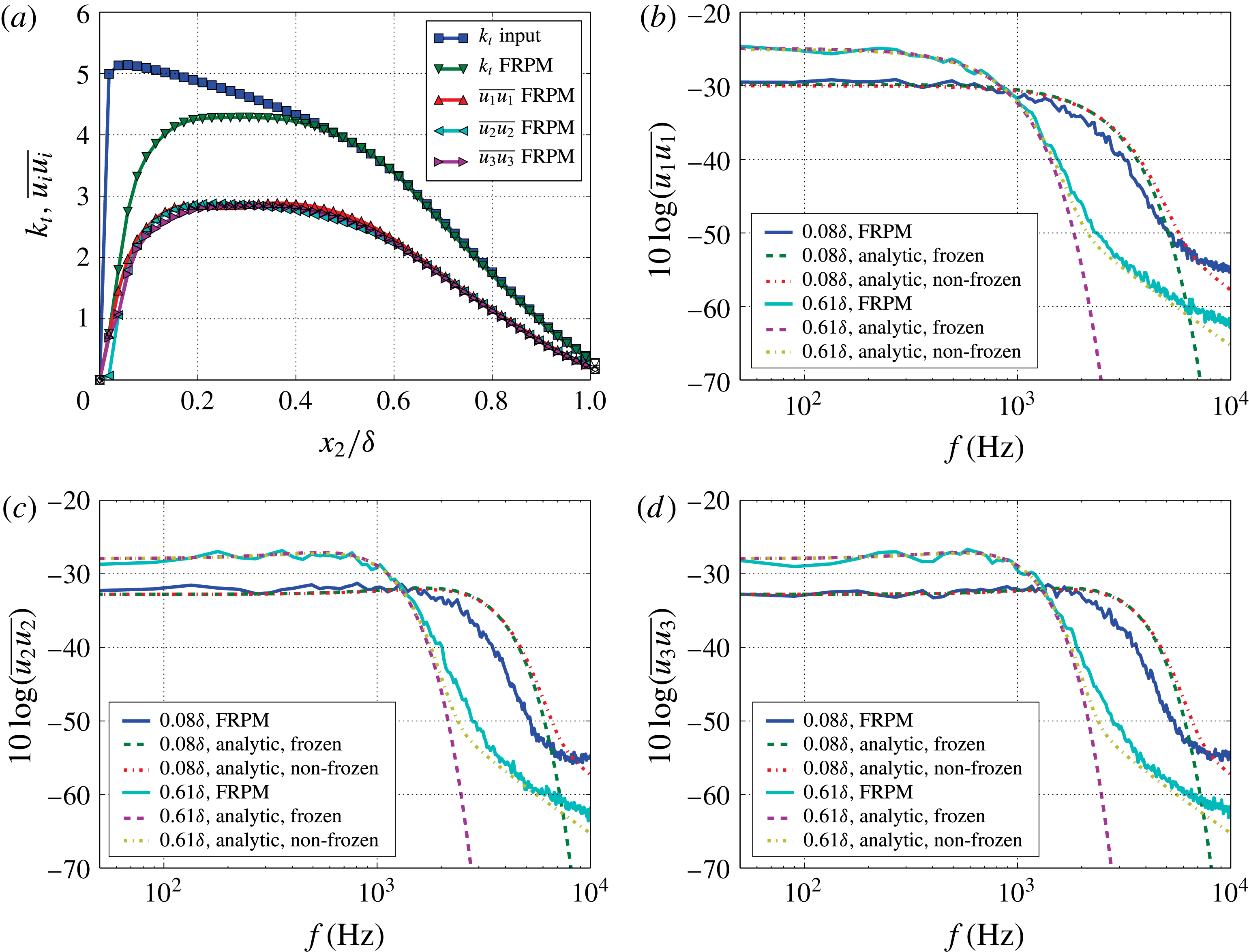
. Furthermore, an isotropic scaling according to (2.24) is used. Figure 5(a) shows the reconstructed turbulent kinetic energy and the reconstructed variance of the velocity fluctuations for the
 $Ma=0.1$
flow in comparison to the target within the boundary layer. The variance of the velocity fluctuations are nearly equally well realised for each component based on the isotropic turbulence approach. In the outer region
 ${>}0.4\unicode[STIX]{x1D6FF}$
a perfect reconstruction of the kinetic energy is visible. A lack of kinetic energy level is evident in the region close to the wall, especially for
 ${<}0.1\unicode[STIX]{x1D6FF}$
. The reason for the loss in reconstructed energy is mainly because of a grid resolution not fine enough to resolve the small turbulence structures close to the wall. Note, for a technical application of the method, it is sufficient to resolve structures only in the regime of interest, which typically demands a truncation of the realisation at a smallest resolved length scale (FRPM mesh resolution limit), typically considerably above the Kolmogorov scale. Otherwise, if all scales would be entirely reproduced, the resolution requirement of the mesh would be driven by similar constraints as those present in LES or DNS.
FRPM realises 1-D Gaussian turbulence spectra
 $\unicode[STIX]{x1D6F7}_{ii}(k_{1})$
as analytically derived in appendix B. A relationship between velocity spectra
 $\unicode[STIX]{x1D6F7}_{ij}(\unicode[STIX]{x1D714})$
and
 $\unicode[STIX]{x1D6F7}_{ij}(k_{1})$
is presented by (A 14) in appendix A. The result depends on whether turbulence decay (finite decay time scale
 $\unicode[STIX]{x1D70F}_{s}$
) is considered or if the assumption of frozen turbulence (Taylor’s hypothesis) is applied by choosing
 $\unicode[STIX]{x1D70F}_{s}\rightarrow \infty$
. Practically, considering a uniform mean flow in the
 $x_{1}$
-direction, the frequency spectrum of frozen turbulence is obtained by replacing wavenumber
 $k_{1}$
by
 $\unicode[STIX]{x1D714}/U_{c}$
, where
 $U_{c}$
is the convection velocity in the
 $x_{1}$
-direction. Figure 5(b–d) shows the realised velocity spectra compared to the analytical Gaussian velocity spectra with frozen and non-frozen turbulence. The spectra are calculated with a window length of 512 samples for the case with the larger time step and 1024 samples for the case with the smaller time step. The sampling rate is 23 kHz and 50 kHz for the larger and smaller time steps, respectively, which results a frequency resolution of approximately 45 Hz and 49 Hz. Furthermore, the spectra are averaged at 3 different positions in the spanwise direction within a distance of
 $2.7\unicode[STIX]{x1D6FF}$
where nearly no correlations of the data between each position exist. The same condition for spectral estimation is made for the wall pressure spectra. Spectra at two different wall-normal positions, viz.
 $x_{2}=0.08\unicode[STIX]{x1D6FF}$
and
 $x_{2}=0.61\unicode[STIX]{x1D6FF}$
, are considered. The realised spectra show an excellent agreement with the analytical results at
 $0.61\unicode[STIX]{x1D6FF}$
. However, at
 $0.08\unicode[STIX]{x1D6FF}$
an attenuation of the spectral magnitude is shown at higher frequencies, e.g. above 2 kHz for spectra of
 $u_{2}$
and
 $u_{3}$
. This is because the used grid cannot resolve small turbulence structures in the near-wall region, which causes the attenuation of kinetic energy reconstruction in this region shown in figure 5(a). As a result of the introduced turbulence decay the non-frozen turbulence spectra present a less steep roll off for higher frequencies compared with that of frozen turbulence. The reason is that the form of the moving axis spectrum
 $\unicode[STIX]{x1D719}_{m}(\unicode[STIX]{x1D714}-U_{c}k_{1})$
changes from
 $\unicode[STIX]{x1D6FF}(\unicode[STIX]{x1D714}-U_{c}k_{1})$
to a broadband form, refer to the discussion in appendix A. As a consequence of an exchange of the
 $\unicode[STIX]{x1D6FF}$
function by a mollified distribution in the convolution integral equation (A 14), the energy of the frozen turbulence spectrum is spread out into the neighbourhood, in this case from the lower frequencies into the higher frequencies. It is worth to note that the spectral contribution from turbulence decay depends on the form of
 $\unicode[STIX]{x1D719}_{m}$
.
Realisation of the velocity fluctuations from FRPM within the boundary layer based on the isotropic turbulence approach; (a) turbulent kinetic energy reconstruction; (b)
 $u_{1}$
spectra; (c)
 $u_{2}$
spectra; (d)
 $u_{3}$
spectra; for frozen (
 $\unicode[STIX]{x1D70F}\rightarrow \infty$
) and non-frozen (
 $\unicode[STIX]{x1D70F}$
from (2.16)) turbulence.

The anisotropy of wall turbulence for the FRPM turbulence realisation is obtained by realising anisotropic Reynolds stress components and using a stretching factor
 $\unicode[STIX]{x1D6FE}$
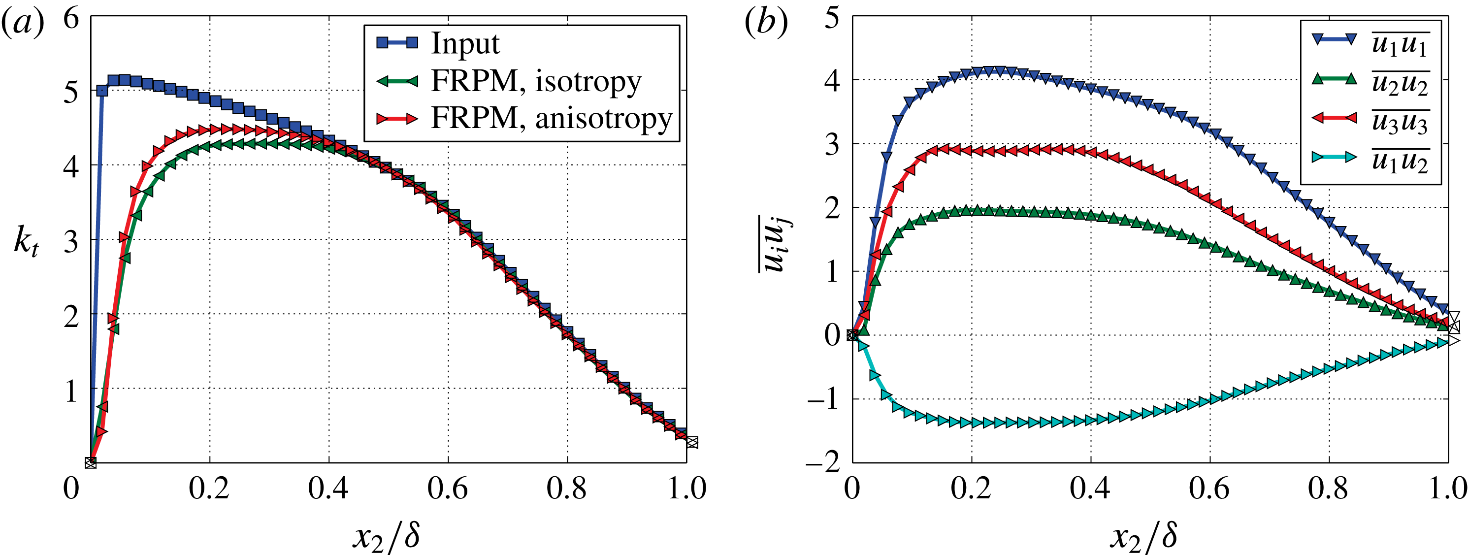
in the integral length scale, refer to § 2.2. Figure 6(a) shows that in the inner region the reconstruction of turbulence kinetic energy with the anisotropic turbulence approach is slightly better than the one with the isotropic turbulence approach. The reason for that could be the applied stretching factor, which causes a larger vortex structure in the streamwise direction and benefits the used FRPM grid owing to the coarsest resolution in the streamwise direction. Figure 6(b) shows the realised Reynolds stress components, the ratio between them follows the ratio from the RANS solution shown in figure 4.
Realisation of the velocity fluctuations from FRPM within the boundary layer with both the isotropic and anisotropic turbulence approach, stretching factor
 $\unicode[STIX]{x1D6FE}=1.5$
; (a) turbulent kinetic energy reconstruction; (b) Reynolds stress tensors.

4.2 One-point spectra
The source term of the Poisson equation (2.1) comprises two contributions, viz. the mean-shear turbulence interaction term and the turbulence–turbulence interaction term. Since the Poisson equation is linear, the solution of pressure fluctuations can be separately solved,
 $$\begin{eqnarray}\displaystyle & \displaystyle p_{ms}^{(I)}(\boldsymbol{x},t)=-2\unicode[STIX]{x1D70C}_{0}\int _{\boldsymbol{V}_{\boldsymbol{s}}+\boldsymbol{V}_{\boldsymbol{s}}^{\prime }}\frac{\unicode[STIX]{x2202}U_{1}}{\unicode[STIX]{x2202}x_{2}}\frac{\unicode[STIX]{x2202}u_{2}(\boldsymbol{y},t)}{\unicode[STIX]{x2202}x_{1}}\boldsymbol{\cdot }g(\boldsymbol{x}-\boldsymbol{y})\,\text{d}^{3}\boldsymbol{y}, & \displaystyle\end{eqnarray}$$
 $$\begin{eqnarray}\displaystyle & \displaystyle p_{tt}^{(I)}(\boldsymbol{x},t)=-\unicode[STIX]{x1D70C}_{0}\int _{\boldsymbol{V}_{\boldsymbol{s}}+\boldsymbol{V}_{\boldsymbol{s}}^{\prime }}\frac{\unicode[STIX]{x2202}^{2}}{\unicode[STIX]{x2202}x_{i}\unicode[STIX]{x2202}x_{j}}(u_{i}u_{j}-\overline{u_{i}u_{j}})(\boldsymbol{y},t)\boldsymbol{\cdot }g(\boldsymbol{x}-\boldsymbol{y})\,\text{d}^{3}\boldsymbol{y}, & \displaystyle\end{eqnarray}$$
where
 $p_{ms}$
denotes the pressure fluctuations for the mean-shear term and
 $p_{tt}$
for the turbulence–turbulence term. Index
 $(I)$
denotes the options to realise the integral. Integration by parts allows to shift the derivatives acting on terms with fluctuating velocity to the Green function, providing two other options:
 $$\begin{eqnarray}\displaystyle & \displaystyle p_{ms}^{(II)}(\boldsymbol{x},t)=2\unicode[STIX]{x1D70C}_{0}\int _{\boldsymbol{V}_{\boldsymbol{s}}+\boldsymbol{V}_{\boldsymbol{s}}^{\prime }}\frac{\unicode[STIX]{x2202}U_{1}}{\unicode[STIX]{x2202}x_{2}}u_{2}(\boldsymbol{y},t)\boldsymbol{\cdot }\frac{\unicode[STIX]{x2202}g(\boldsymbol{x}-\boldsymbol{y})}{\unicode[STIX]{x2202}x_{1}}\,\text{d}^{3}\boldsymbol{y}, & \displaystyle\end{eqnarray}$$
 $$\begin{eqnarray}\displaystyle & \displaystyle p_{tt}^{(II)}(\boldsymbol{x},t)=\unicode[STIX]{x1D70C}_{o}\int _{\boldsymbol{V}_{\boldsymbol{s}}+\boldsymbol{V}_{\boldsymbol{s}}^{\prime }}\frac{\unicode[STIX]{x2202}}{\unicode[STIX]{x2202}x_{i}}(u_{i}u_{j}-\overline{u_{i}u_{j}})(\boldsymbol{y},t)\boldsymbol{\cdot }\frac{\unicode[STIX]{x2202}g(\boldsymbol{x}-\boldsymbol{y})}{\unicode[STIX]{x2202}x_{j}}\,\text{d}^{3}\boldsymbol{y}, & \displaystyle\end{eqnarray}$$
 $$\begin{eqnarray}\displaystyle & \displaystyle p_{tt}^{(III)}(\boldsymbol{x},t)=-\unicode[STIX]{x1D70C}_{0}\int _{\boldsymbol{V}_{\boldsymbol{s}}+\boldsymbol{V}_{\boldsymbol{s}}^{\prime }}(u_{i}u_{j}-\overline{u_{i}u_{j}})(\boldsymbol{y},t)\boldsymbol{\cdot }\frac{\unicode[STIX]{x2202}^{2}g(\boldsymbol{x}-\boldsymbol{y})}{\unicode[STIX]{x2202}x_{i}\unicode[STIX]{x2202}x_{j}}\,\text{d}^{3}\boldsymbol{y}. & \displaystyle\end{eqnarray}$$
Hence, instead of numerical derivatives of the velocity fluctuations analytical derivatives of the Green function occur. The realised Reynolds stress is taken as input values for
 $\overline{u_{i}u_{j}}$
. Finally, equations (4.1) and (4.3) represent two approaches for
 $p_{ms}$
and equations (4.2), (4.4) and (4.5) give three for
 $p_{tt}$
.
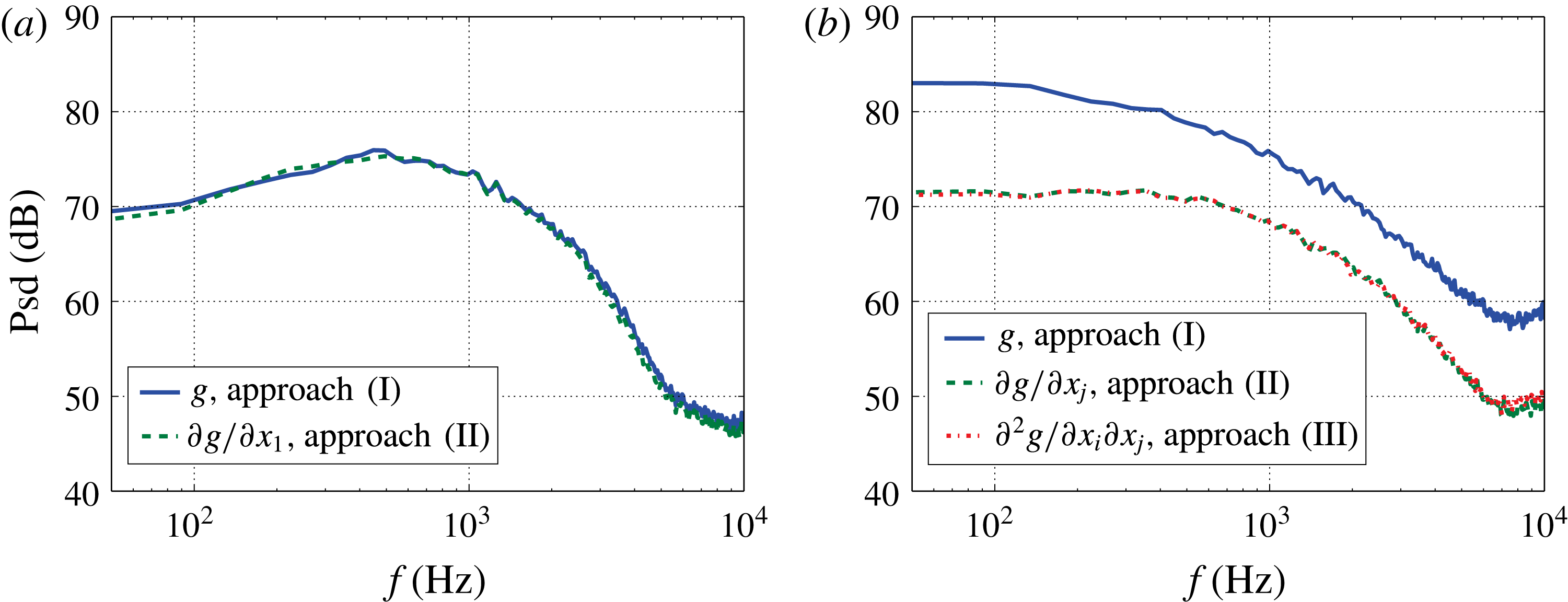
Wall pressure fluctuations for different approaches; (a) spectra for
 $p_{ms}$
; (b) spectra for
 $p_{tt}$
.

Figure 7 shows the one-point spectra for the wall pressure fluctuations at
 $Ma=0.1$
calculated with isotropic turbulence. Both approaches for
 $p_{ms}$
show nearly identical results. This indicates that either the approach with
 $\unicode[STIX]{x2202}u_{2}/\unicode[STIX]{x2202}x_{1}$
or with
 $\unicode[STIX]{x2202}g/\unicode[STIX]{x2202}x_{1}$
is well suited for the given computational set-up. Comparable results for
 $p_{tt}$
are obtained for both approaches using
 $\unicode[STIX]{x2202}g/\unicode[STIX]{x2202}x_{j}$
or
 $\unicode[STIX]{x2202}^{2}g/\unicode[STIX]{x2202}x_{i}\unicode[STIX]{x2202}x_{j}$
, respectively. In contrast, large discrepancies are obtained by the approach with
 $\unicode[STIX]{x2202}^{2}(u_{i}u_{j}-\overline{u_{i}u_{j}})/\unicode[STIX]{x2202}x_{i}\unicode[STIX]{x2202}x_{j}\cdot g$
. This is because of the involved numerical errors by calculating the double derivative
 $\unicode[STIX]{x2202}^{2}/\unicode[STIX]{x2202}x_{2}\unicode[STIX]{x2202}x_{2}$
in the last couple of cell layers close to the wall.
To avoid the singularity of the Green function a minimum threshold
 $r_{min}$
is applied. The value of
 $r_{min}$
is set to be equal to the mesh size in the
 $x_{2}$
-direction which is the finest resolution of the used grid. Note that, the local pressure fluctuations within the boundary layer can be altered by the choice of
 $r_{min}$
for approaches involving
 $g$
or
 $\unicode[STIX]{x2202}^{2}g/\unicode[STIX]{x2202}x_{i}\unicode[STIX]{x2202}x_{j}$
. In contrast, the approach with
 $\unicode[STIX]{x2202}g/\unicode[STIX]{x2202}x_{j}$
is independent of
 $r_{min}$
, insofar its value is not larger than the smallest mesh size of the used grid. From the results for
 $p_{ms}$
and
 $p_{tt}$
and the good solution for the singularity problem, it is concluded that the approach based on
 $\unicode[STIX]{x2202}g/\unicode[STIX]{x2202}x_{j}$
provides the best consistent numerical realisation. Thus,
 $p_{total}$
is calculated with
 $$\begin{eqnarray}\displaystyle p_{total}(\boldsymbol{x},t) & = & \displaystyle p_{ms}^{(II)}(\boldsymbol{x},t)+p_{tt}^{(II)}(\boldsymbol{x},t)=\unicode[STIX]{x1D70C}_{o}\int _{\boldsymbol{V}_{\boldsymbol{s}}+\boldsymbol{V}_{\boldsymbol{s}}^{\prime }}\left\{2\frac{\unicode[STIX]{x2202}U_{1}}{\unicode[STIX]{x2202}x_{2}}u_{2}(\boldsymbol{y},t)\boldsymbol{\cdot }\frac{\unicode[STIX]{x2202}g(\boldsymbol{x}-\boldsymbol{y})}{\unicode[STIX]{x2202}x_{1}}\right.\nonumber\\ \displaystyle & & \displaystyle +\left.\frac{\unicode[STIX]{x2202}}{\unicode[STIX]{x2202}x_{i}}(u_{i}u_{j}-\overline{u_{i}u_{j}})(\boldsymbol{y},t)\boldsymbol{\cdot }\frac{\unicode[STIX]{x2202}g(\boldsymbol{x}-\boldsymbol{y})}{\unicode[STIX]{x2202}x_{j}}\right\}\text{d}^{3}\boldsymbol{y}.\end{eqnarray}$$
Theoretically, the wall pressure spectrum for
 $p_{ms}$
defined by
 $\unicode[STIX]{x1D6F7}_{ppms}(\unicode[STIX]{x1D714})$
can be analytically solved for statistically stationary turbulence using the mean-flow one-point statistics together with the two-point cross-correlation model that underlies the synthetic turbulence generation. Following Blake (Reference Blake1986), the solution of (4.1) becomes,
 $$\begin{eqnarray}\displaystyle \unicode[STIX]{x1D6F7}_{ppms}(\unicode[STIX]{x1D714}) & = & \displaystyle 4\unicode[STIX]{x1D70C}_{0}^{2}\int _{0}^{\unicode[STIX]{x1D6FF}}\int _{-\infty }^{\infty }\int _{-\infty }^{\infty }\frac{k_{1}^{2}}{k^{2}}\exp (-2kx_{2})\overline{u_{2}^{2}}(x_{2})\frac{\unicode[STIX]{x2202}U_{1}^{2}(x_{2})}{\unicode[STIX]{x2202}x_{2}}\unicode[STIX]{x1D6EC}_{2}(x_{2})\nonumber\\ \displaystyle & & \displaystyle \times \,\unicode[STIX]{x1D6F7}_{22}(k_{1},k_{3},x_{2})\unicode[STIX]{x1D719}_{m}(\unicode[STIX]{x1D714}-k_{1}U_{c}(x_{2}))\,\text{d}k_{1}\,\text{d}k_{3}\,\text{d}x_{2},\end{eqnarray}$$
where
 $k_{i}$
is wavenumber component in each direction and
 $k^{2}=k_{1}^{2}+k_{3}^{2}$
. The quantity of
 $\overline{u_{2}^{2}}(x_{2})$
is the turbulence variance in wall-normal direction,
 $U_{1}(x_{2})$
is the local flow velocity and
 $U_{c}(x_{2})$
is the local flow convective velocity. For the present problem with convection in the
 $x_{1}$
-direction and assumed statistical stationary in
 $x_{1}$
,
 $U_{c}(x_{2})$
can be calculated from the maximum of the cross-correlation function
 $R_{uu}(\unicode[STIX]{x0394}x_{1},0,\unicode[STIX]{x1D70F})$
, the convective velocity follows from
 $U_{c}=\unicode[STIX]{x0394}x_{1}/\unicode[STIX]{x1D70F}(\unicode[STIX]{x0394}x_{1})$
, where
 $\unicode[STIX]{x1D70F}$
is the time shift for the velocity fluctuations at which
 $R_{uu}$
is maximal, and
 $\unicode[STIX]{x0394}x_{1}$
indicates the two-point separation in the
 $x_{1}$
-direction. The local convective velocity
 $U_{c}(x_{2})$
is obtained using the simulation data. The results indicate
 $U_{c}(x_{2})=U_{1}(x_{2})$
across the boundary layer. The same results were reported by Wooldridge & Willmarth (Reference Wooldridge and Willmarth1962) through measuring the correlation between the velocity fluctuations and the wall pressure fluctuations. In (4.7)
 $\unicode[STIX]{x1D6EC}_{2}(x_{2})$
is the double-sided correlation length in the wall-normal direction, i.e.
 $\unicode[STIX]{x1D6EC}_{2}(x_{2})=2l_{s}(x_{2})$
, where
 $l_{s}$
is the integral length scale used in FRPM. The velocity wavenumber spectrum of the vertical fluctuating velocity
 $\unicode[STIX]{x1D6F7}_{22}(k_{1},k_{3},x_{2})$
can be obtained by
 $\int \unicode[STIX]{x1D6F7}_{22}(k_{1},k_{2},k_{3},x_{2})\,\text{d}k_{2}$
. The form of
 $\unicode[STIX]{x1D6F7}_{22}(k_{1},k_{2},k_{3})$
for FRPM is represented in appendix B. The function
 $\unicode[STIX]{x1D719}_{m}(\unicode[STIX]{x1D714}-k_{1}U_{c}(x_{2}))$
is the moving axis spectrum which in FRPM is implicitly defined through the turbulence decay term
 $\exp (-\unicode[STIX]{x1D70F}/\unicode[STIX]{x1D70F}_{s})$
, ref to (A 11).
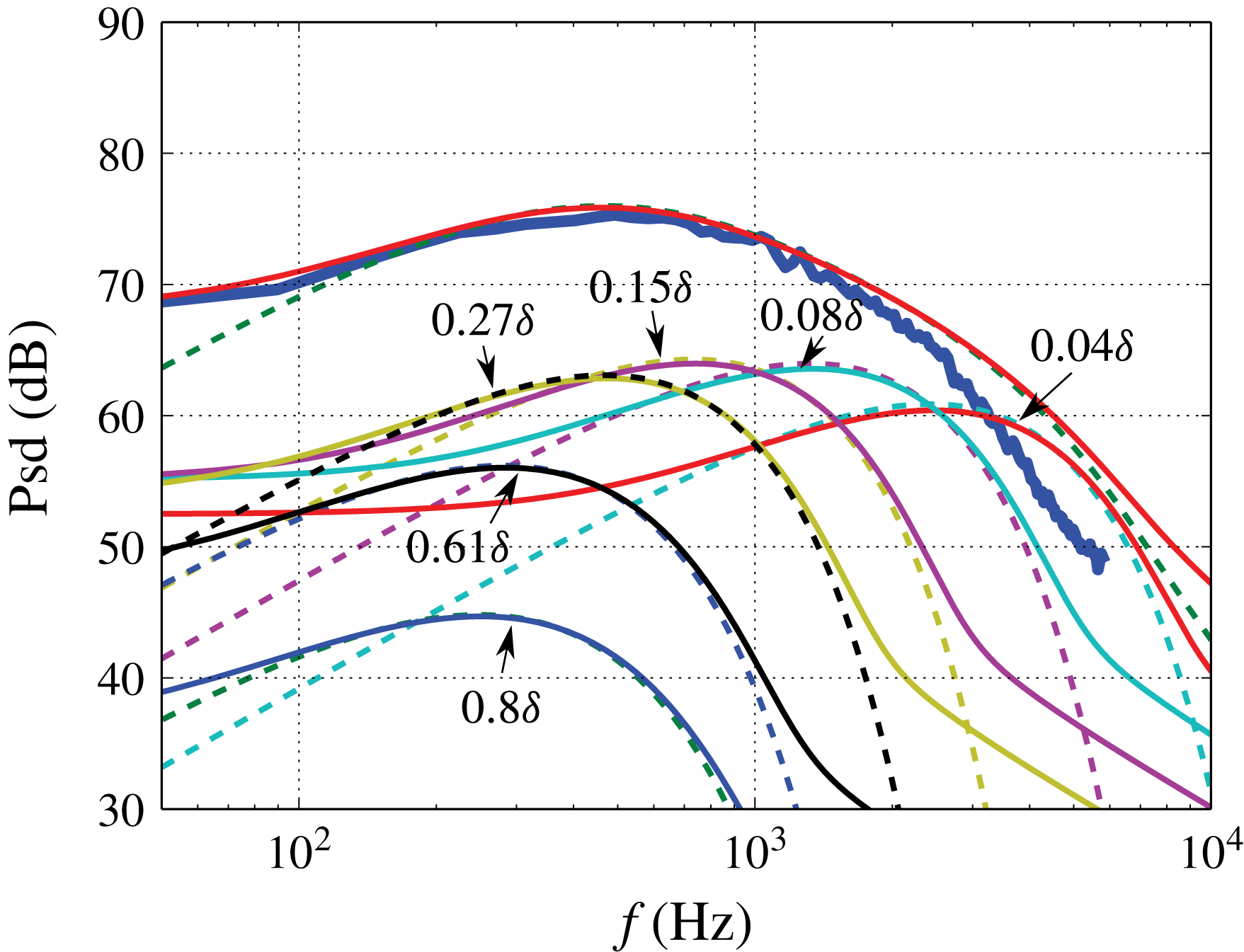
Figure 8 shows an excellent agreement at low and medium frequencies between the theoretical prediction for the non-frozen turbulence and the simulated spectrum. Discrepancies between the theoretical and simulated spectra are found for frequencies above 2 kHz due to the attenuation of the realised velocity fluctuation spectra, see figure 5(c). Equation (4.7) provides the wall pressure spectrum as an integral over all decks of the boundary layer. The theoretical contributions to the wall pressure fluctuations from different wall-normal positions are also presented in figure 8. This shows that positions closer to the wall are responsible for the higher frequencies. For example, the position at
 $0.08\unicode[STIX]{x1D6FF}$
has a large contribution for frequencies 1–2 kHz. The outer region at
 $0.61\unicode[STIX]{x1D6FF}$
shows only little relevance to the wall pressure fluctuations. Due to the term
 $k_{1}^{2}/k^{2}\exp (-2kx_{2})$
in (4.7) the contribution of the boundary layer to the wall pressure spectra especially vanishes at lower and higher frequencies. For example the maximum contributions of the boundary layer at
 $0.08\unicode[STIX]{x1D6FF}$
and
 $0.61\unicode[STIX]{x1D6FF}$
are located around 1.5 kHz and 300 Hz, respectively. If we compare these contributions with the theoretical velocity fluctuation spectra of
 $u_{2}$
in the boundary layer shown in figure 5(c), it is interesting to find that the maximum contributions occur in the plateau region of the
 $\overline{u_{2}u_{2}}$
spectrum. This indicates that the energy-containing range of the spectrum dominates the contribution to the wall pressure fluctuations, and the inertial subrange, not well represented by the realised Gaussian spectrum due to the rapid roll off at higher frequencies, only plays a minor role. Unlike for velocity spectra, for which the impact of turbulence decay is primarily found at high frequencies, the turbulence decay increases the contributions to the pressure spectra at low frequencies as well. Consequently, the near-wall region becomes also relevant to wall pressure fluctuations at low frequencies. Note that, a flatter slope than the classic
 $\unicode[STIX]{x1D714}^{2}$
rise is visible at low frequencies as a result of the turbulence decay.
Wall pressure fluctuations for
 $p_{ms}$
and the contributions to the wall pressure fluctuations from different positions at
 $0.04\unicode[STIX]{x1D6FF}$
,
 $0.08\unicode[STIX]{x1D6FF}$
,
 $0.15\unicode[STIX]{x1D6FF}$
,
 $0.27\unicode[STIX]{x1D6FF}$
,
 $0.61\unicode[STIX]{x1D6FF}$
and
 $0.8\unicode[STIX]{x1D6FF}$
; (——), numerical result; (——), theoretical results for non-frozen turbulence; (– – –), theoretical results for frozen turbulence.

Wall pressure spectra for (——),
 $p_{ms}$
; (– – –),
 $p_{tt}$
; (— ⋅ —),
 $p_{total}$
; (a) isotropic turbulence approach; (b) anisotropy of Reynolds stress tensors; (c) anisotropy of Reynolds stress tensors and length scale anisotropy with
 $\unicode[STIX]{x1D6FE}=1.5$
; (d) anisotropy of Reynolds stress tensors and length scale anisotropy with
 $\unicode[STIX]{x1D6FE}=2$
.

Figure 9 shows the calculated spectra for
 $p_{ms}$
,
 $p_{tt}$
and
 $p_{total}$
at
 $Ma=0.1$
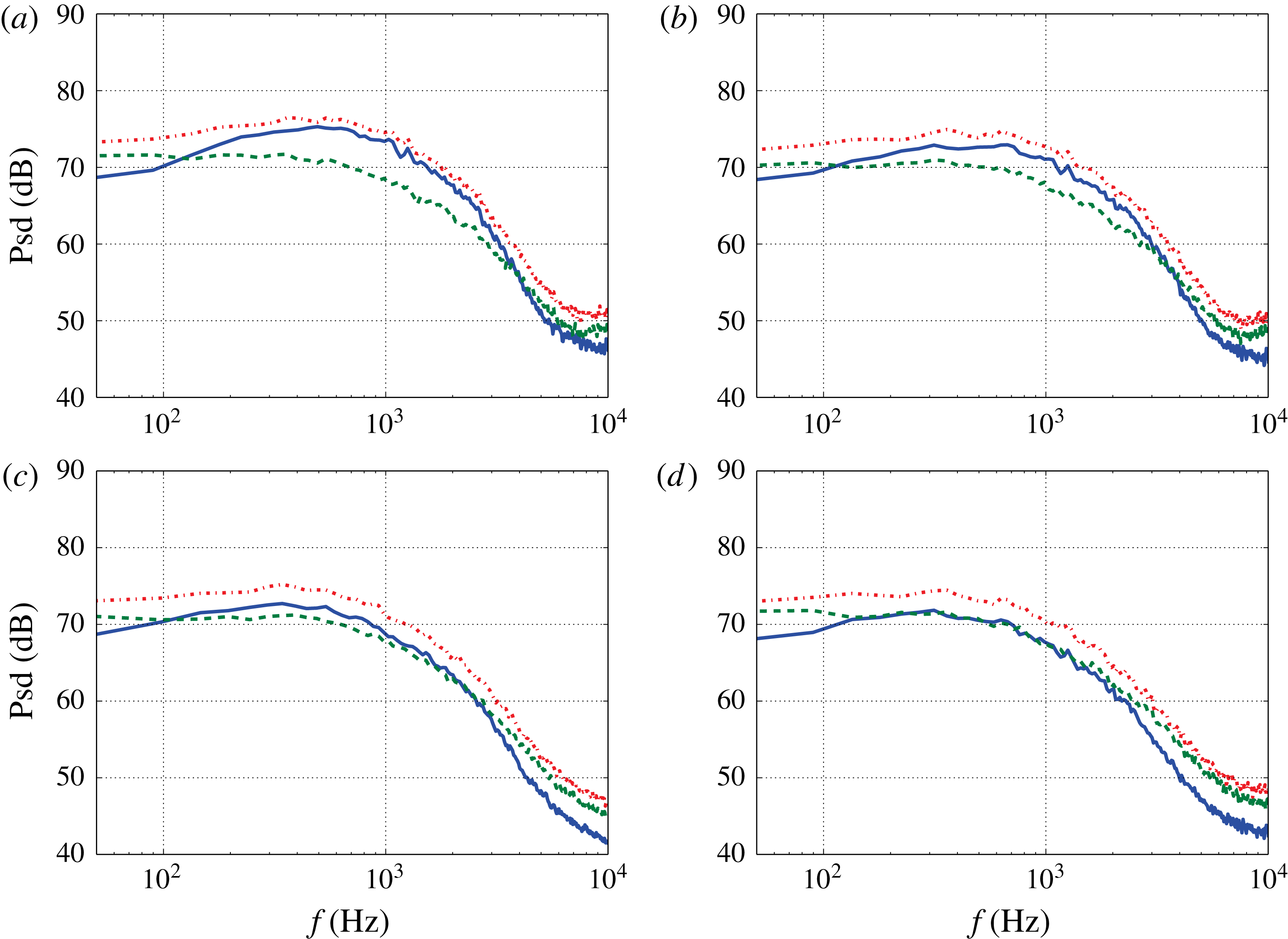
with the different isotropic and anisotropic turbulence approaches. The
 $p_{ms}$
spectra show a maximum at medium frequencies and an increase behaviour at low frequencies because of the derivative in the streamwise direction
 $\unicode[STIX]{x2202}/\unicode[STIX]{x2202}x_{1}$
of the mean-shear source term. In contrast, the
 $p_{tt}$
spectra own a low-pass behaviour with a maximum plateau at low frequencies. This is mainly attributed to the turbulence–turbulence source terms with the double derivatives in the spanwise and wall-normal directions, i.e.
 $\unicode[STIX]{x2202}^{2}/\unicode[STIX]{x2202}x_{2}\unicode[STIX]{x2202}x_{2}$
,
 $\unicode[STIX]{x2202}^{2}/\unicode[STIX]{x2202}x_{2}\unicode[STIX]{x2202}x_{3}$
and
 $\unicode[STIX]{x2202}^{2}/\unicode[STIX]{x2202}x_{3}\unicode[STIX]{x2202}x_{3}$
. Due to this behaviour, the
 $p_{tt}$
spectra gain dominance at low frequencies. It is noteworthy to mention that above 2 kHz the realised velocity fluctuation spectra decay due to the mesh size, refer to figure 5. Therefore, comparison and discussion of both spectra are restricted in the frequency range below 2 kHz. At medium frequencies from where the maximum amplitude for the
 $p_{ms}$
spectrum is located at 2 kHz, both
 $p_{ms}$
and
 $p_{tt}$
show similar trends.
The importance of both
 $p_{ms}$
and
 $p_{tt}$
is impacted by the anisotropy of turbulence. The maximum difference of spectral amplitude between the two terms is found for the isotropic turbulence approach, where the
 $p_{ms}$
is approximately 5 dB larger than the
 $p_{tt}$
at medium frequencies. The difference becomes smaller when the anisotropy of Reynolds stress is applied and even disappears when an anisotropic length scale is applied. Note that, the spectral amplitude for
 $p_{tt}$
is hardly impacted by the anisotropy of the turbulence. In contrast, for
 $p_{ms}$
the amplitude decreases when anisotropy of Reynolds stress and length scale anisotropy are applied. Reason for that could be
 $p_{tt}$
is driven by the turbulence kinetic energy, however,
 $p_{ms}$
only by the
 $u_{2}$
which is more sensitively altered by the anisotropy of turbulence. Another effect of the anisotropy is that the maximum of
 $p_{ms}$
spectra shifts to a lower frequency. This is probably due to the anisotropy of Reynolds stress tensor
 $\overline{u_{1}u_{2}}$
. This correlates the velocity fluctuations
 $u_{1}$
which contain more energy at lower frequencies to
 $u_{2}$
. The result with anisotropic Reynolds stress and a length scale stretching factor
 $\unicode[STIX]{x1D6FE}=1.5$
is mostly consistent with the results from Kim (Reference Kim1989) and Chang et al. (Reference Chang, Piomelli and Blake1999), which demonstrated the both terms have the same order for the contribution to the wall pressure fluctuations. The spectral trend of the both terms show also good agreement with the spectra calculated from Kim (Reference Kim1989), which show a flat behaviour at lower frequencies for
 $p_{tt}$
and the maximum of
 $p_{ms}$
is approximately 1 dB above
 $p_{tt}$
levels. Note that, in the present calculation, the velocity fluctuations for
 $u_{1}$
from RANS solutions are smaller than the ones from LES, refer to figure 4(b). This will cause an attenuation of the spectral amplitude for
 $p_{tt}$
. The attenuation at low and medium frequencies is estimated to be less than 0.5 dB.
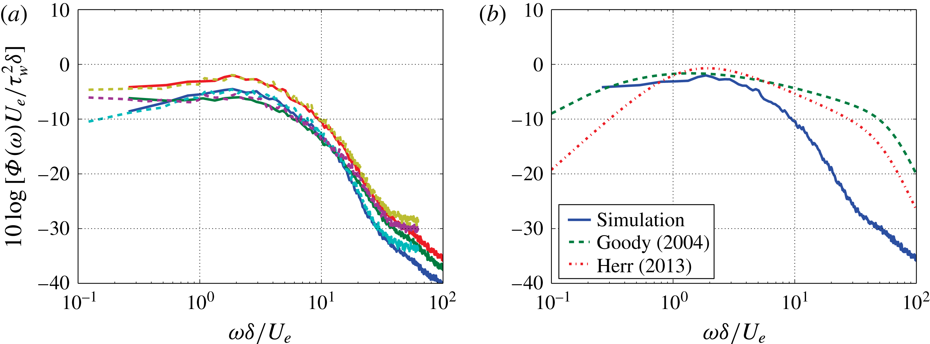
Figure 10(a) shows a spectral scaling between the cases for
 $Ma=0.1$
and
 $Ma=0.2$
. The results are gained with the anisotropic turbulence Reynolds stress and the stretching factor
 $\unicode[STIX]{x1D6FE}=1.5$
and also for the remaining results shown in the paper. All the components
 $p_{ms}$
,
 $p_{tt}$
and
 $p_{all}$
collapse for the calculated velocities. A Reynolds number effect which causes an elongated extension of the spectral slope at medium frequencies as the Reynolds number increases is not found in the present result. This is mainly because the used mesh resolution cannot resolve the fine structure of the turbulence and therefore the Reynolds number effect at higher frequencies cannot be calculated. A comparison between the scaled spectrum for
 $Ma=0.1$
and the wall pressure model spectra is shown in figure 10(b). At medium frequencies the calculated spectrum shows good agreement with the models. However, at higher frequencies the slope of the calculated spectrum departs from
 $\unicode[STIX]{x1D714}^{-0.7}$
from the Goody (Reference Goody2004) model and
 $\unicode[STIX]{x1D714}^{-1}$
from the Herr (Reference Herr2013) model, which is due to the lack of the realised turbulent kinetic energy in the near-wall region. Also a different trend is found at low frequencies. The models have a
 $\unicode[STIX]{x1D714}^{2}$
behaviour at low frequencies which is based on the mean-shear part for a frozen turbulence.
Wall pressure fluctuations; (a) scaled spectra for
 $p_{ms}$
,
 $p_{tt}$
and
 $p_{total}$
for (——),
 $Ma=0.1$
and (– – –),
 $Ma=0.2$
; (b) comparison between the numerical result and the models.

4.3 Root mean square pressure
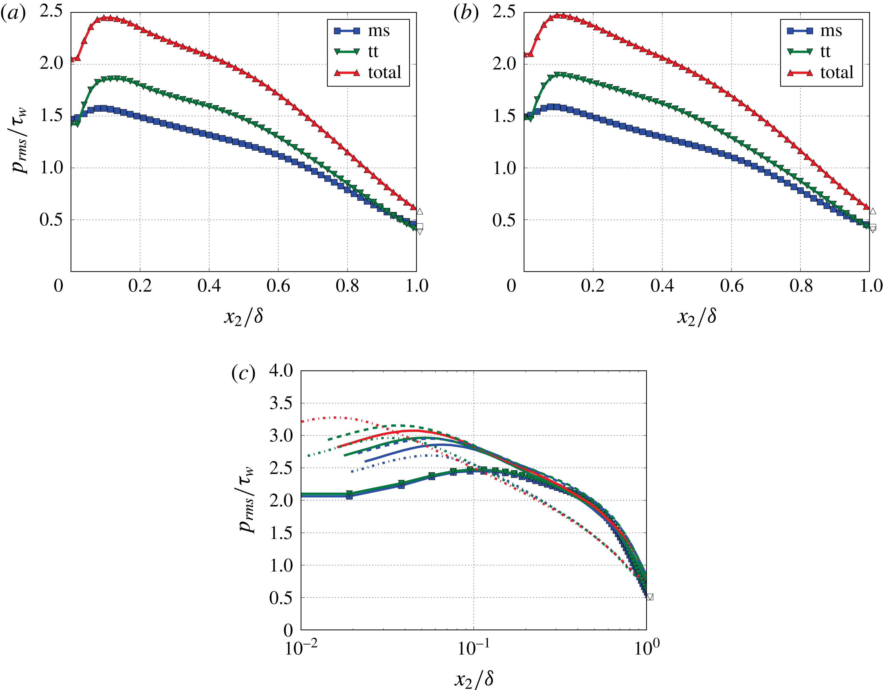
Figure 11(a,b) shows the root mean square value of pressure fluctuations for
 $p_{ms}$
,
 $p_{tt}$
and
 $p_{total}$
normalised by the wall shear stress
 $\unicode[STIX]{x1D70F}_{w}$
across the boundary layer. The pressure fluctuations show very similar trends for both velocities. At the wall the magnitude for
 $p_{ms}$
and
 $p_{tt}$
are of the same order and within the boundary layer the magnitude of
 $p_{tt}$
is larger than
 $p_{ms}$
. A similar trend is also found by Kim (Reference Kim1989).
A comparison between the present results for
 $p_{total}$
and results from the literature is shown in figure 11(c). The present results show an excellent agreement with the results from Schlatter et al. (Reference Schlatter, Örlü, Li, Fransson, Johansson, Alfredsson and Henningson2009) and Jiménez et al. (Reference Jiménez, Hoyas, Simens and Mizuno2010) in the outer region
 ${>}0.3\unicode[STIX]{x1D6FF}$
. However, approaching the wall, the discrepancies become larger due to the lack of the realised kinetic energy, as shown in figure 6(a). A Reynolds number effect is visible in the results from the literature that increases the maximum value of the pressure fluctuations and shifts the maximum position closer to the wall as the Reynolds number increases. The increase of magnitude is mainly caused by the fine-scale turbulence and its produced energy at higher frequencies, e.g. an elongated extension of the
 $\unicode[STIX]{x1D714}^{-0.7}$
or
 $\unicode[STIX]{x1D714}^{-1}$
slope to higher frequencies for the wall pressure fluctuations. However, this effect is not found in the present study due to the limited mesh resolution used.
Root mean square of pressure fluctuations across the boundary layer, calculated with anisotropy of Reynolds stress tensors and length scale anisotropy with
 $\unicode[STIX]{x1D6FE}=1.5$
; (a) trend of
 $p_{rms}/\unicode[STIX]{x1D70F}_{w}$
for
 $p_{ms}$
,
 $p_{tt}$
and
 $p_{total}$
for
 $Ma=0.1$
,
 $Re_{\unicode[STIX]{x1D70F}}=2513$
; (b) trend of
 $p_{rms}/\unicode[STIX]{x1D70F}_{w}$
for
 $p_{ms}$
,
 $p_{tt}$
and
 $p_{total}$
for
 $Ma=0.2$
,
 $Re_{\unicode[STIX]{x1D70F}}=4357$
; (c) comparison for
 $p_{total}$
between the present results and results from literature over logarithmic scale; (–▪–), (–▾–), present calculation,
 $Re_{\unicode[STIX]{x1D70F}}=2513$
and
 $Re_{\unicode[STIX]{x1D70F}}=4357$
; (——), Jiménez et al. (Reference Jiménez, Hoyas, Simens and Mizuno2010),
 $Re_{\unicode[STIX]{x1D70F}}=445{-}690$
; (– – –), Schlatter et al. (Reference Schlatter, Örlü, Li, Fransson, Johansson, Alfredsson and Henningson2009),
 $Re_{\unicode[STIX]{x1D70F}}=500$
and
 $Re_{\unicode[STIX]{x1D70F}}=800$
; (— ⋅ —), Hoyas & Jiménez (Reference Hoyas and Jiménez2006),
 $Re_{\unicode[STIX]{x1D70F}}=550{-}2003$
.

4.4 Broadband correlations
The space–time correlation of the pressure fluctuations is defined by
 $$\begin{eqnarray}R_{pp}(\boldsymbol{x},\boldsymbol{r},\unicode[STIX]{x1D70F})=\langle p(\boldsymbol{x},t)p(\boldsymbol{x}+\boldsymbol{r},t+\unicode[STIX]{x1D70F})\rangle .\end{eqnarray}$$
For the calculation domain the boundary layer grows slowly, so the flow field can be treated as a homogeneous field. Hence,
 $R_{pp}(\boldsymbol{x},\boldsymbol{r},\unicode[STIX]{x1D70F})\simeq R_{pp}(\boldsymbol{r},\unicode[STIX]{x1D70F})$
.
4.4.1 Longitudinal space–time correlation and mean convective velocity
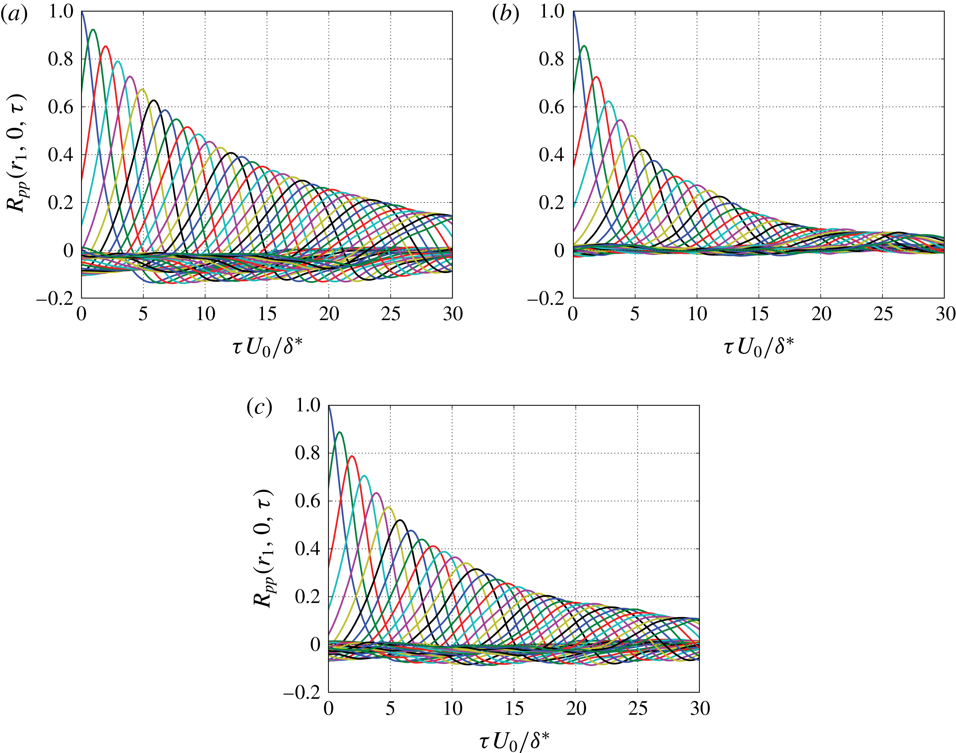
Figure 12 shows the results for longitudinal space–time correlation for
 $p_{ms}$
,
 $p_{tt}$
and
 $p_{total}$
according to (4.8) with
 $p(\boldsymbol{x},t)$
derived from (4.6). The analysis for the two-point statistics herein and the rest of the paper is based on the results from the
 $Ma=0.1$
flow. The correlation for
 $p_{tt}$
drops off much faster than for
 $p_{ms}$
, because the turbulence decay acts stronger on the second-order turbulence–turbulence term. The correlation decay for
 $p_{total}$
is in between
 $p_{ms}$
and
 $p_{tt}$
and derived as a weighted average from the two parts. The correlation curves become broader with increasing
 $r_{1}$
. This is because the smaller eddies close to the wall with lower velocities decay stronger than the larger eddies with higher velocities. Consequently, the correlation at larger
 $r_{1}$
is rather dominated by the larger eddies.
Longitudinal space–time correlation as a function of
 $\unicode[STIX]{x1D70F}U_{0}/\unicode[STIX]{x1D6FF}^{\ast }$
for fixed space increments,
 $r_{1}=0.68\unicode[STIX]{x1D6FF}^{\ast }{-}25\unicode[STIX]{x1D6FF}^{\ast }$
with an increment of
 $0.68\unicode[STIX]{x1D6FF}^{\ast }$
; (a) mean-shear contribution to
 $R_{pp}(r_{1},0,\unicode[STIX]{x1D70F})$
; (b) turbulence–turbulence contribution to
 $R_{pp}(r_{1},0,\unicode[STIX]{x1D70F})$
; (c) combined contribution to
 $R_{pp}(r_{1},0,\unicode[STIX]{x1D70F})$
.

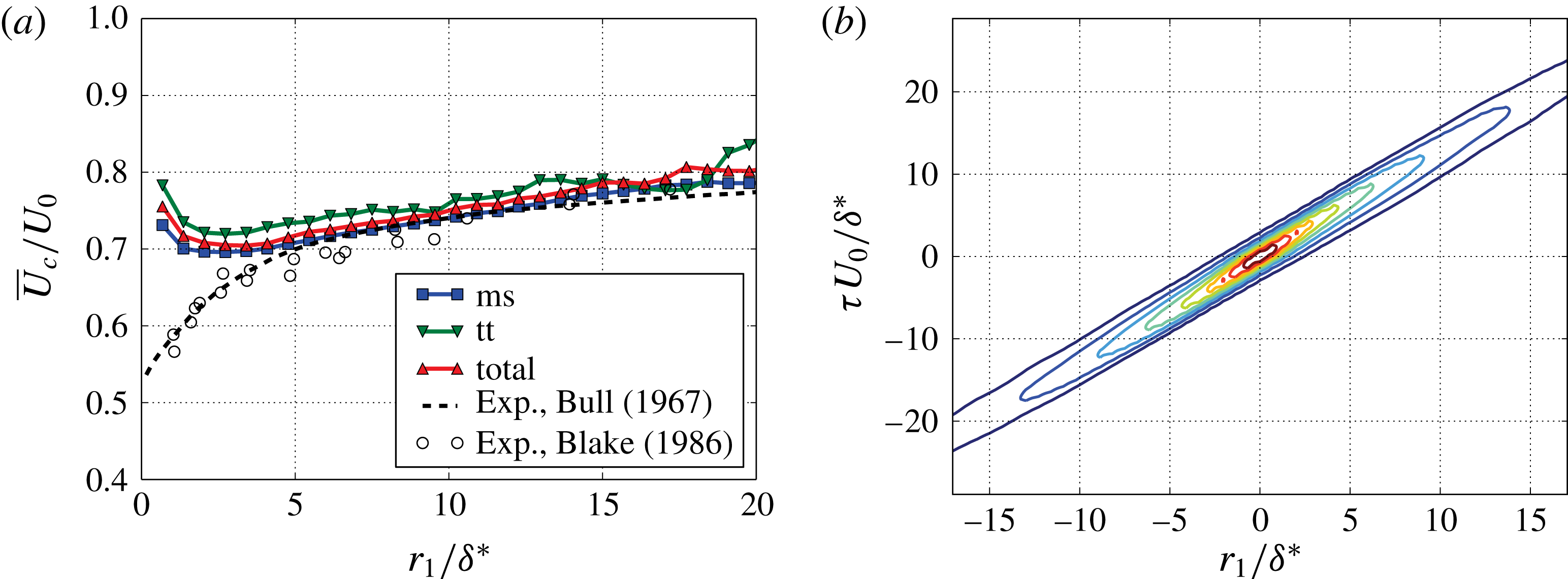
(a) Mean convective velocity
 $\overline{U}_{c}(r_{1})$
; (b) contour plot of longitudinal space–time correlation.

Mean convective velocity
 $\overline{U}_{c}$
can be estimated by using the time shift
 $\unicode[STIX]{x1D70F}$
of the maximum correlation for a fixed distance
 $r_{1}$
,
 $\overline{U}_{c}(r_{1})=r_{1}/\unicode[STIX]{x1D70F}(r)$
. The results shown in figure 13(a) illustrate a growth of
 $\overline{U}_{c}$
with increasing distances. This indicates the larger eddies with higher velocities dominate progressively at larger
 $r_{1}$
. The trend for
 $p_{total}$
fits well to the measured results from Bull (Reference Bull1967) and Blake (Reference Blake1970) at larger distances, however, at closer distances
 $r_{1}/\unicode[STIX]{x1D6FF}^{\ast }<5$
the present results show larger velocities. The reason is the lack of energy at higher frequencies in the present calculation, since the small eddies moving with lower speed are primarily responsible for the higher frequency range. However, at the very closest distance the convective velocity goes up. The reason for that is not clear to the authors. In general, the convective velocity for
 $p_{tt}$
shows a larger value than
 $p_{ms}$
, which may indicate that the source for
 $p_{tt}$
for the wall pressure fluctuations at low and medium frequencies is located a little further away from the wall than the source for
 $p_{ms}$
.
Figure 13(b) shows the contour plot of longitudinal space–time correlation for
 $p_{total}$
. The iso-contour lines have an elongated shape with two distinct apexes of specific distance
 $r_{1}/\unicode[STIX]{x1D6FF}^{\ast }$
to the origin of the plot. Contours of different apex distances are twisted against each other, resulting in a growing convection velocity with increasing distance
 $r_{1}/\unicode[STIX]{x1D6FF}^{\ast }$
. The asymmetrical and broadened correlation at larger
 $r_{1}$
known from experimental results can also be seen in this contour plot.
4.4.2 Spatial correlation
For
 $\unicode[STIX]{x1D70F}=0$
, we can calculate the spatial correlation
 $R_{pp}(r_{1},r_{3},0)$
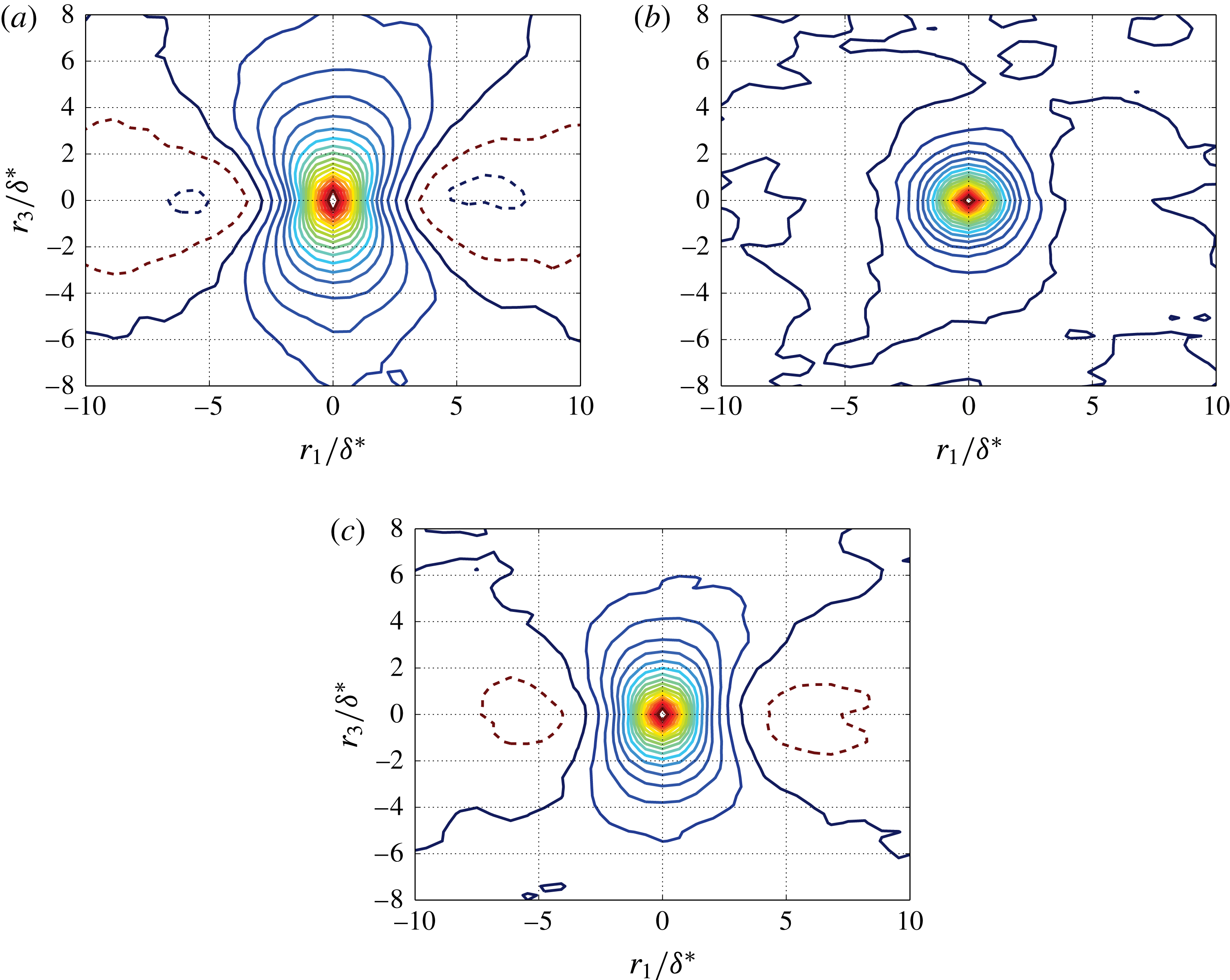
. Results shown in figure 14 represent similar contour shapes between
 $p_{ms}$
and
 $p_{total}$
. Their contour plots illustrate an elongated shape of iso-correlated curves in the lateral direction and a negative correlation region in the longitudinal direction. In contrast,
 $p_{tt}$
exhibits isotropic correlation characteristics. The results for
 $p_{total}$
show good agreement with the data by Bull (Reference Bull1967, Exp.), Viazzo et al. (Reference Viazzo, Dejoan and Schiestel2001, LES) and Gloerfelt & Berland (Reference Gloerfelt and Berland2013, LES).
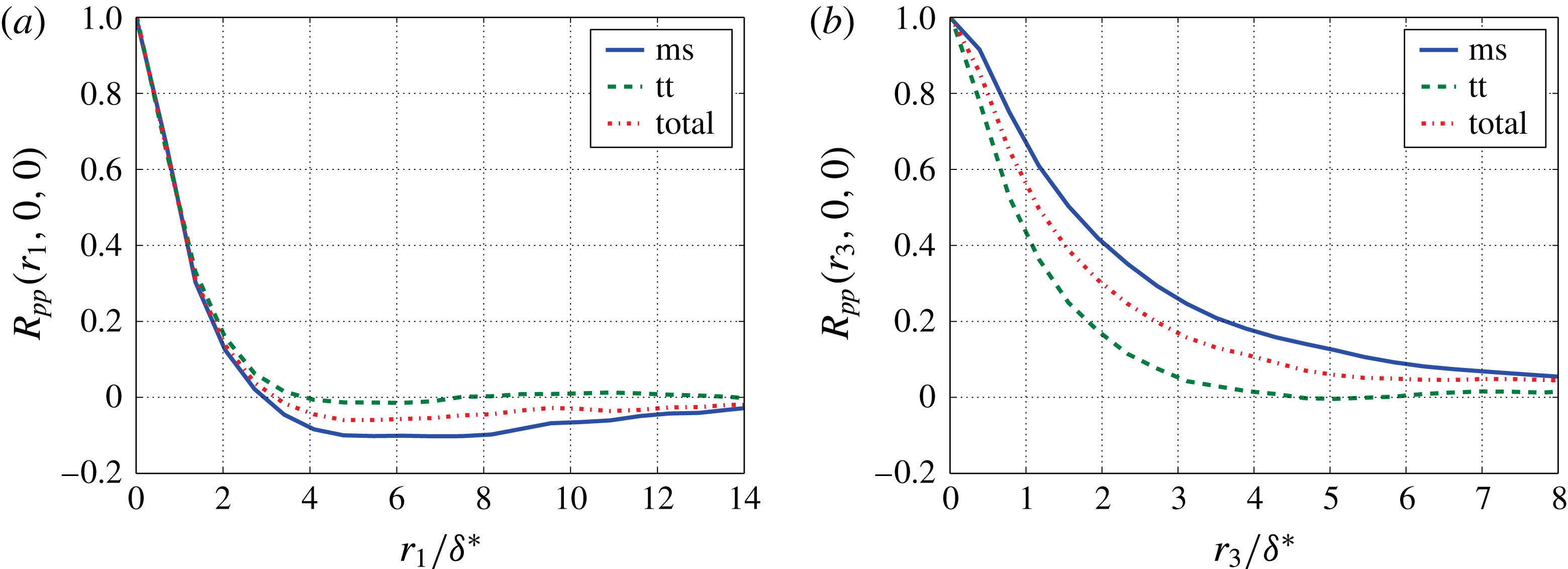
Plots of longitudinal and lateral correlation are shown in figure 15. In the lateral direction the correlation of
 $p_{tt}$
is much shorter than
 $p_{ms}$
. An overshoot with negative value of
 $p_{ms}$
is present in flow direction. This is caused by the streamwise derivative of the velocity fluctuations
 $u_{2}$
. The correlation
 $\langle pu_{2}\rangle$
yields a value of zero for a point underneath the vortex core at the wall and exhibits an odd-shaped distribution in streamwise direction relative to point zero. After reaching the maximum the correlation drops slowly down to zero. As a consequence of this shape, the correlation
 $\langle p\unicode[STIX]{x2202}u_{2}/\unicode[STIX]{x2202}x_{1}\rangle$
exhibits a ‘Mexican hat’ shape in up- and downstream directions and therefore yields negative dips for the streamwise spatial wall pressure correlation.
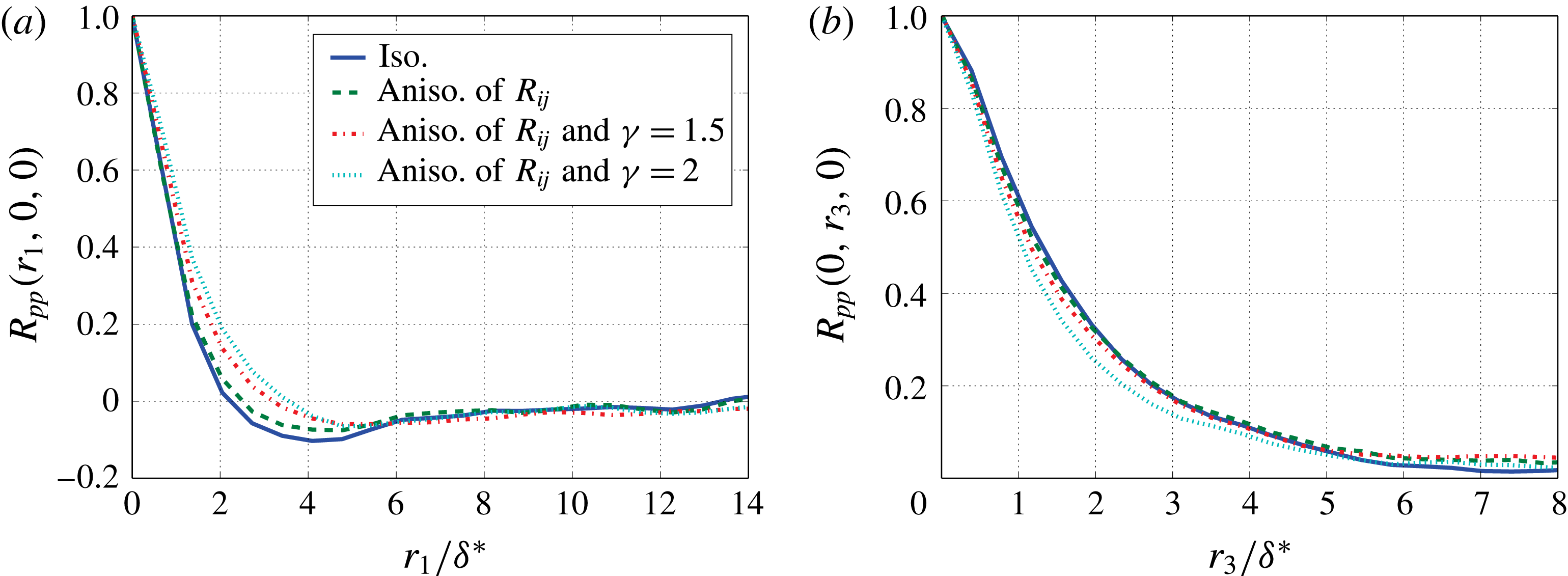
Figure 16 shows the comparison between different turbulence approaches for the longitudinal and lateral correlations. For the anisotropic turbulence, an increase in the longitudinal direction and a decrease in the lateral direction of the correlation are found compared to the isotropic case.
Contour plots of spatial correlation; (——), iso-contours, 0 to 0.9 with increment of 0.05; (– – –), iso-contours,
 $-0.05$
and
 $-0.1$
; (a) mean-shear contribution to
 $R_{pp}(r_{1},r_{3},0)$
; (b) turbulence–turbulence contribution to
 $R_{pp}(r_{1},r_{3},0)$
; (c) combined contribution to
 $R_{pp}(r_{1},r_{3},0)$
.

Spatial correlation for
 $p_{ms}$
,
 $p_{tt}$
and
 $p_{total}$
; (a) longitudinal spatial correlation
 $R_{pp}(r_{1},0,0)$
; (b) lateral spatial correlation
 $R_{pp}(0,r_{3},0)$
.

Spatial correlation for
 $p_{total}$
with different turbulence approaches; (a) longitudinal spatial correlation
 $R_{pp}(r_{1},0,0)$
; (b) lateral spatial correlation
 $R_{pp}(0,r_{3},0)$
.

4.5 Cross-spectra and phase velocities
Cross-spectra are calculated by taking Fourier transform of
 $\unicode[STIX]{x1D70F}$
for the space–time correlation
 $R_{pp}(\boldsymbol{x},\boldsymbol{r},\unicode[STIX]{x1D70F})$
. Based on the Fourier transform, as specified in appendix A, the cross-spectrum reads,
 $$\begin{eqnarray}\unicode[STIX]{x1D6F7}_{pp}(\boldsymbol{x},\boldsymbol{r},\unicode[STIX]{x1D714})=\frac{1}{2\unicode[STIX]{x03C0}}\int _{-\infty }^{\infty }R_{pp}(\boldsymbol{x},\boldsymbol{r},\unicode[STIX]{x1D70F})\exp (-\text{i}\unicode[STIX]{x1D714}\unicode[STIX]{x1D70F})\,\text{d}\unicode[STIX]{x1D70F}.\end{eqnarray}$$
If
 $\boldsymbol{r}=0$
, we obtain the one-point spectrum
 $\unicode[STIX]{x1D6F7}_{pp}(\boldsymbol{x},\unicode[STIX]{x1D714})$
at location
 $\boldsymbol{x}$
. The coherence spectrum is defined by
 $$\begin{eqnarray}\unicode[STIX]{x1D6E4}(\boldsymbol{x},\boldsymbol{r},\unicode[STIX]{x1D714})=\frac{\unicode[STIX]{x1D6F7}_{pp}(\boldsymbol{x},\boldsymbol{r},\unicode[STIX]{x1D714})}{\sqrt{|\unicode[STIX]{x1D6F7}_{pp}(\boldsymbol{x},\boldsymbol{ 0},\unicode[STIX]{x1D714})|}\sqrt{|\unicode[STIX]{x1D6F7}_{pp}(\boldsymbol{x},\boldsymbol{ r},\unicode[STIX]{x1D714})|}},\end{eqnarray}$$
and the phase velocity can be calculated by
 $$\begin{eqnarray}U_{c}(r_{1},\unicode[STIX]{x1D714})=\frac{r_{1}\unicode[STIX]{x1D714}}{\unicode[STIX]{x1D703}(r_{1},\unicode[STIX]{x1D714})},\end{eqnarray}$$
where
 $\unicode[STIX]{x1D703}(r_{1},\unicode[STIX]{x1D714})$
is the phase difference of
 $\unicode[STIX]{x1D6E4}(r_{1},0,\unicode[STIX]{x1D714})$
. Phase velocities and coherence are calculated with a window length of 512 samples, resulting a frequency resolution of approximately 98 Hz. The velocities increase first and after arriving at the maximum fall gradually at higher frequencies, as shown in figure 17. The small
 $U_{c}$
at low frequencies may be caused by the contributions of the small eddies close to the wall moving with slower velocities. The maximum
 $U_{c}/U_{0}$
reaches approximately 0.8 and occurs in the region where the highest energy of the wall pressure fluctuations is contained. Similar trends were measured by Farabee & Casarella (Reference Farabee and Casarella1991), Leclercq & Bohineust (Reference Leclercq and Bohineust2002), Hu & Herr (Reference Hu and Herr2016). In their measurements lower phase velocities for smaller distances were reported, which are not or only weakly present in the calculated results due to the lack of the contribution from the slowly moving small eddies.
Phase velocities as a function of
 $\unicode[STIX]{x1D714}\unicode[STIX]{x1D6FF}/U_{e}$
for fixed space increments,
 $r_{1}=1.36\unicode[STIX]{x1D6FF}^{\ast }{-}8.18\unicode[STIX]{x1D6FF}^{\ast }$
with an increment of
 $1.36\unicode[STIX]{x1D6FF}^{\ast }$
.

Longitudinal coherence as a function of
 $\unicode[STIX]{x1D714}r_{1}/U_{c}$
for fixed space increments,
 $r_{1}=1.36\unicode[STIX]{x1D6FF}^{\ast }{-}8.18\unicode[STIX]{x1D6FF}^{\ast }$
with an increment of
 $1.36\unicode[STIX]{x1D6FF}^{\ast }$
; (– – –),
 $\exp (-\unicode[STIX]{x1D6FC}\unicode[STIX]{x1D714}r_{1}/U_{c})$
with
 $\unicode[STIX]{x1D6FC}=0.125$
; (a) coherence for
 $p_{ms}$
; (b) coherence for
 $p_{tt}$
; (c) coherence for
 $p_{total}$
.

Lateral coherence as a function of
 $\unicode[STIX]{x1D714}r_{1}/U_{c}$
for fixed space increments,
 $r_{3}=0.78\unicode[STIX]{x1D6FF}^{\ast }{-}2.73\unicode[STIX]{x1D6FF}^{\ast }$
with an increment of
 $0.39\unicode[STIX]{x1D6FF}^{\ast }$
; (– – –),
 $\exp (-\unicode[STIX]{x1D6FD}\unicode[STIX]{x1D714}r_{1}/U_{c})$
with
 $\unicode[STIX]{x1D6FD}=0.7$
; (a) coherence for
 $p_{ms}$
; (b) coherence for
 $p_{tt}$
; (c) coherence for
 $p_{total}$
.

Figures 18 and 19 show the longitudinal,
 $\boldsymbol{r}=r_{1}\boldsymbol{\cdot }\boldsymbol{e}_{1}$
, and the lateral coherence,
 $\boldsymbol{r}=r_{3}\boldsymbol{\cdot }\boldsymbol{e}_{3}$
, as a function of
 $\unicode[STIX]{x1D714}r_{1,3}/U_{c}(r_{1},\unicode[STIX]{x1D714})$
. In the spanwise direction
 $U_{c}(\unicode[STIX]{x1D714})$
for the closest distance is used. At larger value of
 $\unicode[STIX]{x1D714}r_{1,3}/U_{c}$
the results seem to collapse together. Corcos (Reference Corcos1964) proposed first an exponential function to describe the coherence function,
 $$\begin{eqnarray}|\unicode[STIX]{x1D6E4}(r_{1},r_{3},\unicode[STIX]{x1D714})|=\exp (-\unicode[STIX]{x1D6FC}\unicode[STIX]{x1D714}r_{1}/U_{c})\exp (-\unicode[STIX]{x1D6FD}\unicode[STIX]{x1D714}r_{3}/U_{c}),\end{eqnarray}$$
where
 $\unicode[STIX]{x1D6FC}$
and
 $\unicode[STIX]{x1D6FD}$
are empirically determined decay constants for the longitudinal and lateral directions. In figure 18 a dashed line with
 $\unicode[STIX]{x1D6FC}=0.125$
is plotted, whose value is obtained from Farabee & Casarella (Reference Farabee and Casarella1991), Hu & Herr (Reference Hu and Herr2016) measured at a comparable Reynolds number. Note that, the convection of the turbulent flow results an offset for samples in the streamwise direction and therefore reduces the longitudinal coherence (Palumbo Reference Palumbo2012). To reduce this effect, the mean convective velocities shown in figure 13(a) are used to calculate the time shift due to the flow convection between different streamwise positions. The time shift is compensated when the streamwise coherence is calculated. In the literature, the value of
 $\unicode[STIX]{x1D6FD}$
is found between 0.7 and 0.72 from Bull (Reference Bull1967), Blake (Reference Blake1986), Hu & Herr (Reference Hu and Herr2016). The present results for coherence show good agreement with the results from the literature.
The comparison between
 $p_{ms}$
and
 $p_{tt}$
show that the coherence decays stronger for
 $p_{tt}$
than for
 $p_{ms}$
in both longitudinal and lateral directions. This impacts the results for
 $p_{total}$
for different turbulence approaches due to the different ratio of
 $p_{ms}$
and
 $p_{tt}$
. In general, the more the
 $p_{tt}$
term contains, the stronger the coherence decays. The value of
 $\unicode[STIX]{x1D6FC}$
is found between 0.9 and 1.35 for the isotropic turbulence approach and the anisotropic turbulence with stretching factor
 $\unicode[STIX]{x1D6FE}=2$
, and
 $\unicode[STIX]{x1D6FD}$
is between 0.45 and 0.72. The lateral coherence is also impacted by the length scale stretching which the coherence decreases as the stretching factor
 $\unicode[STIX]{x1D6FE}$
increases.
Note that, at low values of
 $\unicode[STIX]{x1D714}r_{1,3}/U_{c}$
, the curves do not follow the Corcos model approaching 1, but rather decay. One explanation could be that not only the outer region but also the inner region of the boundary layer contributes significantly to the wall pressure fluctuations at low frequencies, refer to figure 8. Therefore, the decay of the small eddies close to the wall can accelerate the coherence loss at low frequencies.
4.6 Wavenumber–frequency spectra
Wavenumber–frequency spectra are calculated by taking the spatial Fourier transform of the cross-spectra,
 $$\begin{eqnarray}\unicode[STIX]{x1D6F7}_{pp}(k_{1},k_{3},\unicode[STIX]{x1D714})=\frac{1}{(2\unicode[STIX]{x03C0})^{2}}\int _{-\infty }^{\infty }\int _{-\infty }^{\infty }\unicode[STIX]{x1D6F7}_{pp}(r_{1},r_{3},\unicode[STIX]{x1D714})\exp (\text{i}k_{1}r_{1})\exp (\text{i}k_{3}r_{3})\,\text{d}r_{1}\,\text{d}r_{3}.\end{eqnarray}$$
The resolution of the wavenumber domain is defined by
 $\unicode[STIX]{x0394}k_{1}=2\unicode[STIX]{x03C0}/L_{1}$
and
 $\unicode[STIX]{x0394}k_{3}=2\unicode[STIX]{x03C0}/L_{3}$
, where
 $L_{1}$
and
 $L_{3}$
is the longitudinal and lateral array size of the calculation domain for the wavenumber–frequency spectra analysis. In the simulation a virtual microphone array is used with spatial extensions
 $L_{1}\approx 177$
mm and
 $L_{3}\approx 99$
mm. The corresponding values
 $\unicode[STIX]{x0394}k_{1}\approx 17.7~(\text{m}^{-1})$
(coherence in both upstream and downstream directions are considered) and
 $\unicode[STIX]{x0394}k_{3}\approx 63.5~(\text{m}^{-1})$
are too coarse to provide a proper resolution. Unfortunately, the convective ridge is located at a relatively low wavenumber range, especially for low frequencies, e.g. at
 $f=300$
Hz gives
 $k_{1}=\unicode[STIX]{x1D714}/U_{c}\approx 67~(\text{m}^{-1})$
. To reduce the resolution problem, the calculation domain was extended to a spatial extension
 $L_{1}\approx 1062$
mm and
 $L_{3}\approx 396$
mm with zero padding in the appended domain.
Two-dimensional wavenumber–frequency spectra
 $\unicode[STIX]{x1D6F7}_{pp}(k_{1},\unicode[STIX]{x1D714})$
can be obtained by integrating over
 $k_{3}$
,
 $$\begin{eqnarray}\unicode[STIX]{x1D6F7}_{pp}(k_{1},\unicode[STIX]{x1D714})=\int _{-\infty }^{\infty }\unicode[STIX]{x1D6F7}_{pp}(k_{1},k_{3},\unicode[STIX]{x1D714})\,\text{d}k_{3}.\end{eqnarray}$$
(a) Contour plots of wavenumber–frequency spectra
 $\unicode[STIX]{x1D6F7}_{pp}(k_{1},k_{3},\unicode[STIX]{x1D714})$
at 686 Hz; (b) contour plots of wavenumber–frequency spectra
 $\unicode[STIX]{x1D6F7}_{pp}(k_{1},\unicode[STIX]{x1D714})$
.

Figure 20(a) shows the contour plot of
 $\unicode[STIX]{x1D6F7}_{pp}(k_{1},k_{3},\unicode[STIX]{x1D714})$
for
 $p_{total}$
at
 $f=686$
Hz. The convective ridge is well identified and shows good agreement with the measured data by Arguillat et al. (Reference Arguillat, Ricot, Robert and Bailly2005) and Ehrenfried & Koop (Reference Ehrenfried and Koop2008). The maximum of the convective ridge is located at
 $k_{1}\unicode[STIX]{x1D6FF}\approx 4.4$
, which yields the corresponding convective velocity
 $U_{c}\approx 0.83U_{0}$
. The value shows good agreement with the result obtained by the phase velocities which provides
 $U_{c}\approx 0.8U_{0}$
at
 $f=686$
Hz (
 $\unicode[STIX]{x1D714}\unicode[STIX]{x1D6FF}/U_{e}\approx 3.7$
). The two-dimensional spectra
 $\unicode[STIX]{x1D6F7}_{pp}(k_{1},\unicode[STIX]{x1D714})$
in figure 20(b) reveal the convective nature of the wall pressure fluctuations. The main energy centres at
 $k_{1}\approx \unicode[STIX]{x1D714}/U_{c}$
. The shape of the contour twists to a lower value of
 $\unicode[STIX]{x1D714}\unicode[STIX]{x1D6FF}/U_{e}$
at larger
 $k_{1}\unicode[STIX]{x1D6FF}$
, which implies a slower convective velocity at higher frequencies.
One-dimensional spectra of
 $\unicode[STIX]{x1D6F7}_{pp}(k_{1},0,\unicode[STIX]{x1D714})$
and
 $\unicode[STIX]{x1D6F7}_{pp}(k_{1},\unicode[STIX]{x1D714})$
for single frequencies between
 $98~\text{Hz}\leqslant f\leqslant 686~\text{Hz}$
are shown in figure 21. The spectra tend to be flat at very low wavenumbers of
 $k_{1}$
. This feature was also simulated by Viazzo et al. (Reference Viazzo, Dejoan and Schiestel2001) and Gloerfelt & Berland (Reference Gloerfelt and Berland2013). The dominant energy is located at larger
 $k_{1}\unicode[STIX]{x1D6FF}$
for higher frequencies, which corresponds to the convective velocities.
Wavenumber–frequency spectra between 98 Hz and 686 Hz; (a)
 $\unicode[STIX]{x1D6F7}_{pp}(k_{1},0,\unicode[STIX]{x1D714})$
; (b)
 $\unicode[STIX]{x1D6F7}_{pp}(k_{1},\unicode[STIX]{x1D714})$
.

5 Conclusions
Turbulent wall pressure fluctuations were studied with a model for synthetic turbulence. The wall pressure fluctuations were calculated from a Poisson equation. The equation was solved in the wavenumber domain according to Hockney’s method. Source terms were realised by FRPM. The kinetic energy was well reconstructed except for the near-wall region, especially for
 ${<}0.1\unicode[STIX]{x1D6FF}$
. This is acceptable for the purpose which is orientated to practice applications, because the region close to the wall impacts mostly the high frequencies but not the main features for the wall pressure fluctuations. Moreover, the high frequencies are generally irrelevant to the vibration due to the poor transmission efficiency for the structural response. Both the mean-shear turbulence interaction term and the turbulence–turbulence interaction term were considered. The results demonstrated that the wall pressure fluctuations contributed from both terms are of the same order of magnitude if anisotropic turbulence is considered. For isotropic turbulence the mean-shear term is the dominant term. In contrast to the spectra with a peak out at medium frequencies for the mean-shear term, the spectra for the turbulence–turbulence term show a maximum plateau at lower frequencies. The calculated one-point spectrum for the mean-shear term is verified by comparing to the theoretical prediction using the turbulence statistics provided by FRPM. Compared to the spectral models from the literature a stronger decay at high frequencies was found which is mainly because of the limited grid resolution which was not fine enough to resolve the small turbulence structures close to the wall. The two-point correlation properties were consistent with the database from other investigators. It was found that the small eddies in the inner region could affect the one-point spectra and the two-point correlation properties at low frequencies due to the temporal turbulence decay. The convective velocities were well estimated. Furthermore, the wavenumber–frequency spectra were calculated. The convective ridge can be clearly determined.
Acknowledgements
This work was conducted in the framework of the DLR project CENT. The authors would like to acknowledge C. Appel for providing the RANS calculation for the present simulation.
Appendix A. Temporal turbulence decay
The space–time correlation
 $\unicode[STIX]{x1D619}_{ij}$
of the velocity fluctuations for turbulent flow can be generally formulated as the product of three distinct functions, for convenience the indices
 $ij$
are dropped in the following discussion.
 $$\begin{eqnarray}R(\boldsymbol{r},\unicode[STIX]{x1D70F})=R_{1}(r_{1}-U_{c}\unicode[STIX]{x1D70F})R_{n}(\boldsymbol{r}_{\boldsymbol{n}})R_{m}(\unicode[STIX]{x1D70F}).\end{eqnarray}$$
Here,
 $\boldsymbol{r}_{\boldsymbol{n}}$
represents the surface two-point distance vector with components
 $r_{2}$
and
 $r_{3}$
, which is independent of
 $\unicode[STIX]{x1D70F}$
.
 $R_{m}(\unicode[STIX]{x1D70F})$
is the temporal turbulence decay factor. In our case for decaying turbulence
 $R_{m}(\unicode[STIX]{x1D70F})=\exp (-|\unicode[STIX]{x1D70F}|/\unicode[STIX]{x1D70F}_{s})$
. For frozen turbulence
 $\unicode[STIX]{x1D70F}_{s}\rightarrow \infty$
, hence
 $R_{m}(\unicode[STIX]{x1D70F})\equiv 1$
.
The wavenumber spectrum can be derived by taking the Fourier transform of the space–time correlation using the following definition of the Fourier transforms in space and time,
 $$\begin{eqnarray}\left.\begin{array}{@{}c@{}}\displaystyle f(r)=\int _{-\infty }^{\infty }f(k)\exp (-\text{i}kr)\,\text{d}k,\quad f(k)=\frac{1}{2\unicode[STIX]{x03C0}}\int _{-\infty }^{\infty }f(r)\exp (\text{i}kr)\,\text{d}r,\\ \displaystyle f(\unicode[STIX]{x1D714})=\frac{1}{2\unicode[STIX]{x03C0}}\int _{-\infty }^{\infty }f(t)\exp (-\text{i}\unicode[STIX]{x1D714}t)\,\text{d}t,\quad f(t)=\int _{-\infty }^{\infty }f(\unicode[STIX]{x1D714})\exp (\text{i}\unicode[STIX]{x1D714}t)\,\text{d}\unicode[STIX]{x1D714}.\end{array}\right\}\end{eqnarray}$$
The wavenumber spectrum reads,
 $$\begin{eqnarray}\displaystyle \unicode[STIX]{x1D6F7}(\boldsymbol{k},\unicode[STIX]{x1D714}) & = & \displaystyle \frac{1}{(2\unicode[STIX]{x03C0})^{4}}\int _{-\infty }^{\infty }\int _{-\infty }^{\infty }\int _{-\infty }^{\infty }\int _{-\infty }^{\infty }R(\boldsymbol{r},\unicode[STIX]{x1D70F})\nonumber\\ \displaystyle & & \displaystyle \times \exp (-\text{i}\unicode[STIX]{x1D714}\unicode[STIX]{x1D70F}+\text{i}k_{1}r_{1}+\text{i}k_{2}r_{2}+\text{i}k_{3}r_{3})\,\text{d}r_{1}\,\text{d}r_{2}\,\text{d}r_{3}\,\text{d}\unicode[STIX]{x1D70F}.\end{eqnarray}$$
Since
 $r_{2}$
and
 $r_{3}$
are
 $\unicode[STIX]{x1D70F}$
independent,
 $$\begin{eqnarray}\displaystyle \unicode[STIX]{x1D6F7}(\boldsymbol{k},\unicode[STIX]{x1D714}) & = & \displaystyle \frac{1}{(2\unicode[STIX]{x03C0})^{4}}\int _{-\infty }^{\infty }\int _{-\infty }^{\infty }R_{n}(\boldsymbol{r}_{\boldsymbol{n}})\exp (\text{i}k_{2}r_{2}+\text{i}k_{3}r_{3})\,\text{d}r_{2}\,\text{d}r_{3}\nonumber\\ \displaystyle & & \displaystyle \times \int _{-\infty }^{\infty }\int _{-\infty }^{\infty }R_{1}(r_{1}-U_{c}\unicode[STIX]{x1D70F})R_{m}(\unicode[STIX]{x1D70F})\exp (-\text{i}\unicode[STIX]{x1D714}\unicode[STIX]{x1D70F}+\text{i}k_{1}r_{1})\,\text{d}r_{1}\,\text{d}\unicode[STIX]{x1D70F}.\end{eqnarray}$$
Let
 $\unicode[STIX]{x1D709}:=r_{1}-U_{c}\unicode[STIX]{x1D70F}$
and the wavenumber spectrum of
 $r_{2}$
and
 $r_{3}$
be written as
 $\unicode[STIX]{x1D719}_{n}(\boldsymbol{k}_{\boldsymbol{n}})$
,
 $$\begin{eqnarray}\unicode[STIX]{x1D6F7}(\boldsymbol{k},\unicode[STIX]{x1D714})=\unicode[STIX]{x1D719}_{n}(\boldsymbol{k}_{\boldsymbol{n}})\frac{1}{(2\unicode[STIX]{x03C0})^{2}}\int _{-\infty }^{\infty }\int _{-\infty }^{\infty }R_{1}(\unicode[STIX]{x1D709})\exp (\text{i}k_{1}\unicode[STIX]{x1D709})\,\text{d}\unicode[STIX]{x1D709}R_{m}(\unicode[STIX]{x1D70F})\exp (-\text{i}\unicode[STIX]{x1D714}\unicode[STIX]{x1D70F}+\text{i}k_{1}U_{c}\unicode[STIX]{x1D70F})\,\text{d}\unicode[STIX]{x1D70F},\end{eqnarray}$$
where
 $$\begin{eqnarray}\unicode[STIX]{x1D719}_{n}(\boldsymbol{k}_{\boldsymbol{n}})=\frac{1}{(2\unicode[STIX]{x03C0})^{2}}\int _{-\infty }^{\infty }\int _{-\infty }^{\infty }R_{n}(\boldsymbol{r}_{\boldsymbol{n}})\exp (\text{i}k_{2}r_{2}+\text{i}k_{3}r_{3})\,\text{d}r_{2}\,\text{d}r_{3}.\end{eqnarray}$$
In that follows, we can also express the resulting wavenumber spectrum as the product of three contributions,
 $$\begin{eqnarray}\unicode[STIX]{x1D6F7}(\boldsymbol{k},\unicode[STIX]{x1D714})=\unicode[STIX]{x1D719}_{1}(k_{1})\unicode[STIX]{x1D719}_{n}(\boldsymbol{k}_{\boldsymbol{n}})\unicode[STIX]{x1D719}_{m}(\unicode[STIX]{x1D714}-U_{c}k_{1}),\end{eqnarray}$$
where
 $$\begin{eqnarray}\displaystyle & \displaystyle \unicode[STIX]{x1D719}_{1}(k_{1})=\frac{1}{2\unicode[STIX]{x03C0}}\int _{-\infty }^{\infty }R_{1}(\unicode[STIX]{x1D709})\exp (\text{i}k_{1}\unicode[STIX]{x1D709})\,\text{d}\unicode[STIX]{x1D709}, & \displaystyle\end{eqnarray}$$
 $$\begin{eqnarray}\displaystyle & \displaystyle \unicode[STIX]{x1D719}_{m}(\unicode[STIX]{x1D714}-U_{c}k_{1})=\frac{1}{2\unicode[STIX]{x03C0}}\int _{-\infty }^{\infty }R_{m}(\unicode[STIX]{x1D70F})\exp (-\text{i}(\unicode[STIX]{x1D714}-U_{c}k_{1})\unicode[STIX]{x1D70F})\,\text{d}\unicode[STIX]{x1D70F}. & \displaystyle\end{eqnarray}$$
The function
 $\unicode[STIX]{x1D719}_{m}(\unicode[STIX]{x1D714}-U_{c}k_{1})$
is the so-called moving axis spectrum. For frozen turbulent flow (
 $\unicode[STIX]{x1D70F}_{s}\rightarrow \infty$
) the temporal turbulence decay factor is
 $R_{m}=1$
, and since the Fourier transform of the unity function is Dirac delta function (Crighton et al.
Reference Crighton, Dowling, Williams, Heckl and Leppington1992), the moving axis spectrum follows
 $$\begin{eqnarray}\unicode[STIX]{x1D719}_{m}(\unicode[STIX]{x1D714}-U_{c}k_{1})=\unicode[STIX]{x1D6FF}(\unicode[STIX]{x1D714}-U_{c}k_{1}).\end{eqnarray}$$
For non-frozen turbulent flow
 $R_{m}=\exp (-|\unicode[STIX]{x1D70F}|/\unicode[STIX]{x1D70F}_{s})$
. Hence,
 $$\begin{eqnarray}\displaystyle \unicode[STIX]{x1D719}_{m}(\unicode[STIX]{x1D714}-U_{c}k_{1}) & = & \displaystyle \frac{1}{2\unicode[STIX]{x03C0}}\int _{-\infty }^{\infty }\exp \left(-\frac{|\unicode[STIX]{x1D70F}|}{\unicode[STIX]{x1D70F}_{s}}\right)\exp (-\text{i}(\unicode[STIX]{x1D714}-U_{c}k_{1})\unicode[STIX]{x1D70F})\,\text{d}\unicode[STIX]{x1D70F}\nonumber\\ \displaystyle & = & \displaystyle \frac{\unicode[STIX]{x1D70F}_{s}}{\unicode[STIX]{x03C0}(1+(\unicode[STIX]{x1D714}-U_{c}k_{1})^{2}\unicode[STIX]{x1D70F}_{s}^{2})}.\end{eqnarray}$$
Taking the integration of
 $\unicode[STIX]{x1D6F7}(\boldsymbol{k},\unicode[STIX]{x1D714})$
over
 $\boldsymbol{k}$
we can obtain the spectrum in frequency domain,
 $$\begin{eqnarray}\displaystyle \unicode[STIX]{x1D6F7}(\unicode[STIX]{x1D714}) & = & \displaystyle \int _{-\infty }^{\infty }\int _{-\infty }^{\infty }\int _{-\infty }^{\infty }\unicode[STIX]{x1D6F7}(\boldsymbol{k},\unicode[STIX]{x1D714})\,\text{d}k_{1}\,\text{d}k_{2}\,\text{d}k_{3}\nonumber\\ \displaystyle & = & \displaystyle \int _{-\infty }^{\infty }\int _{-\infty }^{\infty }\int _{-\infty }^{\infty }\unicode[STIX]{x1D719}_{1}(k_{1})\unicode[STIX]{x1D719}_{n}(\boldsymbol{k}_{\boldsymbol{n}})\unicode[STIX]{x1D719}_{m}(\unicode[STIX]{x1D714}-U_{c}k_{1})\,\text{d}k_{1}\,\text{d}k_{2}\,\text{d}k_{3}\nonumber\\ \displaystyle & = & \displaystyle \int _{-\infty }^{\infty }\unicode[STIX]{x1D6F7}(k_{1})\unicode[STIX]{x1D719}_{m}(\unicode[STIX]{x1D714}-k_{1}U_{c})\,\text{d}k_{1},\end{eqnarray}$$
where
 $$\begin{eqnarray}\unicode[STIX]{x1D6F7}(k_{1})=\unicode[STIX]{x1D719}_{1}(k_{1})\int _{-\infty }^{\infty }\int _{-\infty }^{\infty }\unicode[STIX]{x1D719}_{n}(\boldsymbol{k}_{\boldsymbol{n}})\,\text{d}k_{2}\,\text{d}k_{3}.\end{eqnarray}$$
Reintroducing indices
 $ij$
and assuming similar turbulent decay for each Reynolds stress component, i.e.
 $R_{m}(\unicode[STIX]{x1D70F})=R_{m(ij)}(\unicode[STIX]{x1D70F})$
. This follows
 $\unicode[STIX]{x1D719}_{m}(\unicode[STIX]{x1D714}-k_{1}U_{c})=\unicode[STIX]{x1D719}_{m(ij)}(\unicode[STIX]{x1D714}-k_{1}U_{c})$
, hence (A 12) becomes,
 $$\begin{eqnarray}\unicode[STIX]{x1D6F7}_{ij}(\unicode[STIX]{x1D714})=\int _{-\infty }^{\infty }\unicode[STIX]{x1D6F7}_{ij}(k_{1})\unicode[STIX]{x1D719}_{m}(\unicode[STIX]{x1D714}-k_{1}U_{c})\,\text{d}k_{1}.\end{eqnarray}$$
Appendix B. Wavenumber spectra of velocity fluctuations
The longitudinal
 $f(r)$
and lateral
 $g(r)$
correlation functions of isotropic turbulence as realised with FRPM read
 $$\begin{eqnarray}\displaystyle & \displaystyle f(r)=\exp \left(-\frac{\unicode[STIX]{x03C0}r^{2}}{4l_{s}^{2}}\right), & \displaystyle\end{eqnarray}$$
 $$\begin{eqnarray}\displaystyle & \displaystyle g(r)=\left(1-\frac{\unicode[STIX]{x03C0}r^{2}}{4l_{s}^{2}}\right)\exp \left(-\frac{\unicode[STIX]{x03C0}r^{2}}{4l_{s}^{2}}\right). & \displaystyle\end{eqnarray}$$
One-dimensional wavenumber spectra can be achieved by taking the Fourier transform of the spatial correlations
 $f(r)$
and
 $g(r)$
,
 $$\begin{eqnarray}\unicode[STIX]{x1D6F7}_{ii}(k_{j})=\left\{\begin{array}{@{}c@{}}\displaystyle \frac{\overline{u_{i}^{2}}}{2\unicode[STIX]{x03C0}}\int _{-\infty }^{\infty }f(r)\exp (-\text{i}k_{j}r)\,\text{d}r,\quad i=j,\\ \displaystyle \frac{\overline{u_{i}^{2}}}{2\unicode[STIX]{x03C0}}\int _{-\infty }^{\infty }g(r)\exp (-\text{i}k_{j}r)\,\text{d}r,\quad i\neq j,\end{array}\right.\end{eqnarray}$$
refer to Batchelor (Reference Batchelor1982). Velocity fluctuation spectra
 $\unicode[STIX]{x1D6F7}_{ij}(\unicode[STIX]{x1D714})$
are related to
 $\unicode[STIX]{x1D6F7}_{ij}(k_{1})$
as introduced by (A 14). Hence to obtain the variance of the velocity fluctuations
 $\overline{u_{i}u_{i}}$
,
 $\unicode[STIX]{x1D6F7}_{ii}(k_{1})$
is of great interest. Specifically, from (B 3) we obtain,
 $$\begin{eqnarray}\displaystyle & \displaystyle \unicode[STIX]{x1D6F7}_{11}(k_{1})=\frac{\overline{u_{1}^{2}}l_{s}}{\unicode[STIX]{x03C0}}\exp \left(\frac{-k_{1}^{2}l_{s}^{2}}{\unicode[STIX]{x03C0}}\right), & \displaystyle\end{eqnarray}$$
 $$\begin{eqnarray}\displaystyle & \displaystyle \unicode[STIX]{x1D6F7}_{22}(k_{1})=\unicode[STIX]{x1D6F7}_{33}(k_{1})=\frac{\overline{u_{2,3}^{2}}l_{s}}{2\unicode[STIX]{x03C0}^{2}}\exp \left(\frac{-k_{1}^{2}l_{s}^{2}}{\unicode[STIX]{x03C0}}\right)(2k_{1}^{2}l_{s}^{2}+\unicode[STIX]{x03C0}). & \displaystyle\end{eqnarray}$$
Three-dimensional wavenumber spectra for isotropic turbulence can be determined by
 $$\begin{eqnarray}\unicode[STIX]{x1D6F7}_{ij}(k_{1},k_{2},k_{3})=\frac{E(k)}{4\unicode[STIX]{x03C0}k^{2}}(\unicode[STIX]{x1D6FF}_{ij}-(k_{i}k_{j})/k^{2}),\end{eqnarray}$$
where
 $k^{2}=k_{1}^{2}+k_{2}^{2}+k_{3}^{2}$
.
 $E(k)$
is the scalar energy spectra and FRPM generated
 $E(k)$
can be written as
 $$\begin{eqnarray}E(k)=\frac{8k_{t}l_{s}^{5}k^{4}}{3\unicode[STIX]{x03C0}^{3}}\exp \left(\frac{-k^{2}l_{s}^{2}}{\unicode[STIX]{x03C0}}\right).\end{eqnarray}$$
Hence the expressions of three-dimensional wavenumber spectra
 $\unicode[STIX]{x1D6F7}_{ii}(k_{1},k_{2},k_{3})$
can be derived. Integrating over
 $k_{2}$
and
 $k_{3}$
we can obtain the one-dimensional wavenumber spectra
 $\unicode[STIX]{x1D6F7}_{ii}(k_{1})$
,
 $$\begin{eqnarray}\unicode[STIX]{x1D6F7}_{ii}(k_{1})=\int _{-\infty }^{\infty }\int _{-\infty }^{\infty }\unicode[STIX]{x1D6F7}_{ii}(k_{1},k_{2},k_{3})\,\text{d}k_{2}\,\text{d}k_{3}.\end{eqnarray}$$
The results are consistent with the form achieved directly from the spatial correlation, equations (B 4) and (B 5).