1. Introduction
Fluids at supercritical pressure have a number of interesting features, including especially high specific heat capacity and no phase change while being heated, which make them attractive working fluid candidates for energy and processing systems. Recent examples of applications include the supercritical water-cooled reactor, currently under development as one of the advanced Generation IV nuclear reactor systems for improved safety, sustainability and efficiency; the supercritical power cycles, which have gained significant interest for use in solar and geothermal systems to improve the cycle efficiency particularly under low temperatures; and the cooling of high heat flux systems including liquid rocket engines with supercritical fuels to achieve high operation temperatures.
Despite no phase changes, the thermophysical properties of fluids at supercritical pressure may undergo strong variations with temperature changes, especially when it crosses the pseudo-critical temperature as the fluid changes from a liquid-like to a gas-like fluid, a process sometimes referred to as pseudo-boiling. As a result, the turbulence dynamics in a flow at supercritical pressure is often very complex and presents significant challenges to predictions.
Heated (or cooled) vertical flows are frequently encountered in practical systems, as well as being fundamental to the understanding of the flow physics of non-isothermal systems. Consequently, the topic has been a focus of many research activities. Notable examples include earlier experimental work by Ackerman (Reference Ackerman1970), Yamagata et al. (Reference Yamagata, Nishikawa, Hasegawa, Fujii and Yoshida1972) and Jackson & Hall (Reference Jackson and Hall1979), the rare but valuable measurements of velocity fields by Kurganov & Kaptil'Ny (Reference Kurganov and Kaptil'Ny1992) and Licht, Anderson & Corradini (Reference Licht, Anderson and Corradini2009) and more recent investigations into different fluids and working conditions (e.g. Bruch, Bontemps & Colasson Reference Bruch, Bontemps and Colasson2009; Liu et al. Reference Liu, Zhu, Yan, Lei, Zhang and Jiang2015). Computational studies have also been carried out more recently aimed at improving the understanding of the flow dynamics and developing engineering prediction tools (e.g. Koshizuka, Takano & Oka Reference Koshizuka, Takano and Oka1995; Cheng, Kuang & Yang Reference Cheng, Kuang and Yang2007; Sharabi et al. Reference Sharabi, Ambrosini, He and Jackson2008; Nemati et al. Reference Nemati, Patel, Boersma and Pecnik2016; Peeters et al. Reference Peeters, Pecnik, Rohde, van der Hagen and Boersma2017; He et al. Reference He, Yan, Wang, Jiang and He2020). A number of review papers have been published on the topic, providing a summary of our understanding to the date of review (Pioro, Khartabil & Duffey Reference Pioro, Khartabil and Duffey2004; Pioro & Duffey Reference Pioro and Duffey2005; Jackson Reference Jackson2013; Yoo Reference Yoo2013). Herein, we avoid repeating their work. Instead, after a brief outline of the basic current knowledge of the turbulence in a heated flow, we focus on the recent developments in the understanding of the flow physics and the scaling of the mean flow and turbulence, mostly developed through direct numerical simulations (DNS), to set the scene for the research described in this paper.
It is now well established that turbulence in a heated vertical flow in a pipe or channel is often significantly different from that in an unheated isothermal flow due to the influence of buoyancy (Jackson Reference Jackson2013; Yoo Reference Yoo2013). In a heated downward (buoyancy-opposed) flow, buoyancy destabilises the flow, enhancing turbulence and heat transfer, whereas the situation is significantly more complex in a heated upward (buoyancy-aided) flow. With moderate buoyancy and heat flux, turbulence is suppressed and heat transfer is worsened. When the heat flux is sufficiently large, resulting in a strong buoyancy, the flow may be completely laminarised leading to the so-called heat transfer deterioration. With a further increase in heat flux and buoyancy, however, turbulence reappears, leading to improved heat transfer. At this stage, the flow is dominated by natural convection. In addition to buoyancy, the flow in a heated pipe is also complicated by the influences of the variations of thermophysical properties, including viscosity and density (other than the buoyancy), which also contribute to the ‘peculiar’ behaviours. It is useful to note that many of the flow physics discussed herein in the context of supercritical fluid also occur in the sub-critical fluid systems, although the fact that the system pressure is above the critical value often makes the phenomena more complex and difficult to predict (McEligot et al. Reference McEligot, Chu, Bae, Laurien and Yoo2020). Bae, Yoo & Choi (Reference Bae, Yoo and Choi2005) carried out one of the first DNS of flow of fluid at supercritical pressure in a vertical pipe for a range of conditions including up and downward flows of variable buoyancy influence. The detailed information on the flow and thermal fields enabled the authors to elaborate the physics on the turbulence reduction and recovery in greater depth than could have been done previously, contributing to the establishment of the general understanding outlined above. The authors studied the external (indirect) and structural (direct) effects of buoyancy on turbulence and turbulent heat flux following Petukhov, Polyakov & Launder (Reference Petukhov, Polyakov and Launder1988). The former refers to the fact that buoyancy acting as a body force modifies the mean velocity profile, which in turn results in a change in turbulence production. This is known to be the dominating effect of the two and key for the primary understanding of such flows, as discussed in the opening paragraphs of this paper. The structural effect on the other hand refers to the effect of the interactions between the fluctuating buoyancy force and velocity, which lead to a direct generation/destruction of turbulence. This is reflected in the budget of turbulence kinetic energy as the buoyancy production. Bae et al. 's (Reference Bae, Yoo and Choi2005) results confirmed that the leading indirect effect could in most cases be used to explain the key features of flow laminarisation and recovery, supporting previous semi-empirical theory. Their data on buoyancy production were, however, proved to be not entirely expected. While the buoyancy production in a downward flow always makes a positive contribution to turbulence kinetic energy as expected, since such a flow is akin to an unstable flow so far as buoyancy is concerned, the production in an upward flow is initially negative, but becomes positive over the rest of the pipe. This was then shown to be the leading factor for turbulence recovery, which is perhaps the main reason that turbulence models are unable to accurately predict turbulence recovery since the buoyancy production is very difficult to predict even with the most sophisticated models (He, Kim & Bae Reference He, Kim and Bae2008; Yoo Reference Yoo2013).
More recently, Peeters et al. (Reference Peeters, Pecnik, Rohde, Van Der Hagen and Boersma2016) conducted DNS of supercritical fluid flow in an annular channel with a heated outer wall and a cooled inner wall with zero net heat flux to the flow, which enabled the authors to study buoyancy aiding and opposing flows simultaneously under an axially fully developed condition. It was shown that the turbulence was significantly decreased near the hot wall but increased near the colder wall, which was only partially attributed to the effect of mean dynamic viscosity and density variations. By analysing the solution of the transport equation for the evolution of the streamwise coherent streak flank strength, the authors demonstrated that, near the hot wall, both thermal expansion and buoyancy reduce the streak coherence, while the viscosity gradient that exists across the streaks may interact with the mean shear to either strengthen or weaken the streaks dependent on the radial location. The formation of the streamwise vortices is not directly strongly influenced by the density and viscosity fluctuations, but is hindered by the torque resulting from the kinetic and density gradients. Overall, based on such analyses of the near-wall turbulence regeneration cycle, the authors concluded that the instantaneous density and dynamic viscosity fluctuations are (partially) responsible for the decreased turbulent motions in the heated fluid, and the increase in the cooled fluid at supercritical pressure. This is consistent with the Bae et al. (Reference Bae, Yoo and Choi2005) conclusion, noting that the buoyancy was moderate in the case of Peeters et al. (Reference Peeters, Pecnik, Rohde, Van Der Hagen and Boersma2016) and the flow was equivalent to the initial phase of Bae et al.'s developing flow.
In a follow-up study (Peeters et al. Reference Peeters, Pecnik, Rohde, van der Hagen and Boersma2017), the authors further analysed the data on the annular flow, specifically focusing on the behaviours of turbulent heat transfer under the influences of the variations of thermal properties. Based on the analyses of the budget of the turbulent heat transfer and quadrant analyses, the authors concluded that both the fluctuations and the mean gradients of the density and molecular Prandtl number had a significant influence on the turbulent heat flux. That is, the direct and indirect effects were equally important under the conditions studied. It was also demonstrated that the temperature fluctuations diminished in the regions of high heat capacity close to the pseudo-critical temperature, reducing the direct effect there, but the opposite was true when the heat capacity was smaller. Azih & Yaras (Reference Azih and Yaras2018) investigated the structural effect of density variations in a heated channel subject to either wall normal, or streamwise (opposed) or zero buoyancy. The heated section was relatively short, just over 11 half-channel heights and hence the flows are typical of those close to the early entrance region of a heated flow. By analysing the coherent turbulence structures, the authors found that the reduction in density and viscosity in a forced convection promotes the generation of small-scale vortices interacting and breaking pre-existing large near-wall structures, hence leading to a reduction in turbulent mixing. In a buoyancy-opposed flow, the baroclinic vorticity generation due to the spanwise density gradient, which was introduced in an earlier study (Reinink & Yaras Reference Reinink and Yaras2015), was shown to promote larger-scale ejections and sweeps leading to additional wall-normal thermal mixing, which is consistent with the findings of previous work under similar conditions (e.g. Bae et al. Reference Bae, Yoo and Choi2005).
Another interesting recent development in the area of heated flows is the scaling of the mean velocity, turbulence and temperature distributions. It is well tested and documented that, for isothermal compressible flows at moderate to high Mach number, the van Driest transformation ( $\bar {u}^{\nu D}=\int _0^{\bar {u}/u_\tau }\sqrt {\bar {\rho }/\bar {\rho }_w}\,\textrm {d}(\bar {u}/u_\tau )$, where
 $\rho\ {\rm and}\ \rho_w $ are density of the fluid in the pipe and at the wall respectively) (Van Driest Reference Van Driest1951) enables the transformed velocity
 $\bar {u}^{\nu D}$ of a compressible flow (in which the viscous heating causes non-uniform mean density distribution) to collapse with the law of the wall of an incompressible flow with
 $y^+$ used in both the compressible and incompressible flows. The transformation adjusts the velocity gradient by a factor of
 $\sqrt {\bar {\rho }/\bar {\rho }_w}$ based on dimensional argument. This transformation works well for boundary layers above an adiabatic wall (Coleman, Kim & Moser Reference Coleman, Kim and Moser1995; Huang, Coleman & Bradshaw Reference Huang, Coleman and Bradshaw1995). The success of the density-weighted scaling can be attributed to the success of the Morkovins hypothesis, which states that the relationships between the relevant statistical properties of turbulence are unaffected by compressibility if the root-mean-square (r.m.s.) density fluctuations are small (of order 1/10) compared with the absolute density (e.g. see Coleman et al. Reference Coleman, Kim and Moser1995; Smits & Dussauge Reference Smits and Dussauge2006).
For a heated flow where there is a wall-normal gradient of thermal properties, the van Driest law fails. This has been attributed to the elongation and shortening of the near-wall streaks on hot and cold walls, respectively (Coleman et al. Reference Coleman, Kim and Moser1995; Duan, Beekman & Martin Reference Duan, Beekman and Martin2010; Lagha et al. Reference Lagha, Kim, Eldredge and Zhong2011). Such streak modifications are quantified based on the wall-based viscous units. To improve the scaling for heated flows, Huang et al. (Reference Huang, Coleman and Bradshaw1995) proposed to use the so-called semi-local scaling, that is, ( $y^*=\bar {\rho }(\tau _w/\bar {\rho })^{1/2}y/\bar {\mu }$, where
 $\tau_w $ is the wall shear stress and
 $\mu $ the dynamic viscosity), which has been found to effectively account for the changes in streak length in the buffer layer (Morinishi, Tamano & Nakabayashi Reference Morinishi, Tamano and Nakabayashi2004; Patel et al. Reference Patel, Peeters, Boersma and Pecnik2015). The modified van Driest law have then been successfully applied to various heated/cooled flow scenarios e.g. Coleman et al. (Reference Coleman, Kim and Moser1995), even though it clearly does not provide a universal law.
Recently, Trettel & Larsson (Reference Trettel and Larsson2016) attempted to develop a universal scaling to consider the influences of variable properties. Their argument was based on the log-layer scaling as well as the near-wall momentum conservation, and introducing velocity and coordinate transformations separately. Their work has resulted in a new velocity transformation accounting for the density and viscosity gradients  $\bar {u}^*=\int _0^{\bar {u}/u_\tau } ({\bar {\rho }}/{\bar {\rho }_w})^{1/2} [1+({1}/{2\bar {\rho }}) ({\textrm {d}\bar {\rho }}/{\textrm {d} y})y -({1}/{ \bar {\mu }}) ({\textrm {d} \bar {\mu }}/{\textrm {d} y}) y ] \,\textrm {d}(\bar {u}/u_\tau )$, which embodies previously proposed scaling, such as the van Driest and that used by Huang et al. (Reference Huang, Coleman and Bradshaw1995).
Pecnik, Patel and colleagues studied the effect of variable properties on turbulence structures and scaling in a series of investigations. Patel et al. (Reference Patel, Peeters, Boersma and Pecnik2015) introduced a semi-local frictional Reynolds number,  $Re_\tau ^* = Re_\tau \sqrt { (\bar {\rho })/\bar {\rho }_w} /(\bar {\mu }/\bar {\mu }_w)$, which was used to successfully rescale turbulence statistics and the van Driest transformed velocity for variable-property flows. The basic expression can be reorganised to take a similar form as that used in Trettel & Larsson (Reference Trettel and Larsson2016) for most flows. Unlike constant-property flows, however, the turbulence statistics show a strong dependence on
 $Re_\tau ^*$. For the case when
 $Re_\tau ^*$ decreases away from the wall, the streamwise normal Reynolds stress anisotropy increases, which was associated with the stretching of the large-scale low-speed streaks in the buffer layer. The reverse is true for increasing
 $Re_\tau ^*$ cases. Later Patel, Boersma & Pecnik (Reference Patel, Boersma and Pecnik2016) provided a more comprehensive discussion on the effects of the near-wall property gradients on mean velocity scaling, near-wall turbulence statistics and turbulence structures. Again
 $Re_\tau ^*$, and in particular, its radial profile, was shown to characterise the modifications of turbulence structures. This was used to explain the way turbulence anisotropy is affected by wall heating and cooling. Additionally, it was found that the viscous shear stress is a universal function in the inner layer when expressed in the semi-local parameter,
 $(h/Re_\tau ^*) \,\textrm {d}u^{\nu D}/{\textrm {d} y}$, where h is half-channel height. It was later shown in Patel, Boersma & Pecnik (Reference Patel, Boersma and Pecnik2017) that the statistics of a scaler (such as temperature) can also be scaled using the semi-local Reynolds number and a semi-local
 $Pr^*$ defined as
 $Pr^*=Pr_w(\bar {\mu }/\mu )/(\overline{\lambda}/\lambda )$. The above idea was further used in Pecnik & Patel (Reference Pecnik and Patel2017) to derive a so-called semi-local scaled transport equation for turbulence kinetic energy, in which the viscous terms are scaled with
 $Re_\tau ^*$ and the turbulence production is governed by the gradient of the van Driest velocity. They then successfully used this equation in conjunction with a turbulence model to simulate several fully developed turbulent flows, ranging from volumetrically heated flows at low Mach (
 $Ma$) numbers to a fully compressible case of
 $Ma=4$ in a channel with isothermal walls.
The above scaling work was based on ordinary fluids (that is fluids at sub-critical pressure). More recently, these scaling theories have been tested for flows at trans-critical and super-critical pressures (Ma, Yang & Ihme Reference Ma, Yang and Ihme2018; Liu et al. Reference Liu, Zhao, Lei, Yang and Nemati2020; Wan et al. Reference Wan, Zhao, Liu, Wang and Lei2020), although all of them only considered forced convection neglecting the effect of buoyancy. Wan et al. (Reference Wan, Zhao, Liu, Wang and Lei2020) found that the semi-local scaling ( $Re_\tau ^*$) correlated both the mean velocity and temperature field very well for a spatially fully developed channel flow with a heated and a cooled wall. Liu et al. (Reference Liu, Zhao, Lei, Yang and Nemati2020) considered a more challenging case where the flow is developing spatially in a heated pipe under a forced convection condition. It was found that the mean velocity in the logarithmic region could be well scaled by the semi-local scaling, but the temperature could be better scaled with the modified van Driest transformation. Ma et al. (Reference Ma, Yang and Ihme2018) considered a flow in a heated/cooled channel with a very high temperature difference (200 K) at a pressure just above the critical value. This hence resulted in a density difference up to 18 times in the flow and therefore an even greater challenge for scaling. It was shown that the semi-local scaling was suitable for one wall, but not the other where the density fluctuations are very high, with a standard deviation of
 $(\rho '/\rho )$ greater than
 $40\,\%$, and hence the condition for the Morkovins hypothesis is not satisfied.
Finally, we briefly discuss the recent work of He, He & Seddighi (Reference He, He and Seddighi2016), which provides much of the foundation of the discussion presented herein. In that work, DNS were carried out to study the effect of non-uniform body force (including, for example, buoyancy force) on turbulence using a prescribed linear or step change body force near the wall. The flow was isothermal. It was established that, in contrast to common perception, the turbulence is not modified by such body forces when compared with that in an equivalent-pressure-gradient (EPG) flow, which can be seen as a suitable reference for the corresponding body-force influenced flows. In this theory, the so-called laminarisation is represented as a reduction in the apparent Reynolds number which can be estimated once the body force itself is known. The detail of the theory is further discussed in the results section. The concept that the buoyancy in a heated flow, which mostly concentrates in the region close to the wall, does not influence the turbulence in the main flow was in fact hypothesised in the early studies of Hall and Jackson in the 1960s, based on which, a widely used heat transfer correlation was developed (refer to the discussion in Jackson Reference Jackson2013). More recently, the apparent Reynolds number concept was used in Marensi, He & Willis (Reference Marensi, He and Willis2021) to produce a Reynolds number–heating phase diagram, showing if a flow is expected to be turbulent or laminar (or convection driven flow) for a heated upward flow based on the Boussinesq approximation. The phase diagram agrees well with DNS results and the analysis of the linear stability.
In the present paper, we aim to establish a unified explanation for the mechanisms of laminarisation due to the effects of buoyancy, and variations of density and viscosity in a heated vertical flow at supercritical pressure. The unified explanation is also applicable to the effect of inertia in such a spatially developing flow, which is treated as a pseudo-body force and its effect is explained in a similar way as for other effects. This work builds upon the understanding and findings on the general behaviours of supercritical fluid flow under strong heating with the effect of buoyancy (both direct and indirect) from previous studies (e.g. Bae et al. Reference Bae, Yoo and Choi2005; Jackson Reference Jackson2013). It also makes use of and extends the understanding on how turbulence is (or is not) influenced by the variations of thermophysical properties (e.g. Patel et al. Reference Patel, Boersma and Pecnik2016; Trettel & Larsson Reference Trettel and Larsson2016) or buoyancy (He et al. Reference He, He and Seddighi2016) with suitably chosen non-dimensional scaling or references. The present work is not aimed at providing a specific scaling scheme per se but its findings can be used to support such development. Additionally, we study the region of ‘full’ laminarisation and show that in this region turbulence in the core of the pipe decays in an exponential manner, similar to that of a grid generated turbulence. Near the wall, however, streaks are generated, which leads to an increase in streamwise turbulent fluctuations (and hence turbulence kinetic energy) but new turbulence (the transverse fluctuating components and turbulence spots) is generated only in a later re-transition region.
2. Methodology
DNS has been carried out using an in-house code CHAPSim, which was developed for isothermal flows (Seddighi Reference Seddighi2011), but has later been extended to solve a low Mach number version of the Navier–Stokes equations together with the energy equation (Wang & He Reference Wang and He2015). The latter is used in this study, which solves the governing equations in the following conservation form in a cylindrical coordinate system:
 \begin{align} &\frac{\partial \rho}{\partial t}+\frac{\partial(\rho u_{z})}{\partial z} + \frac{1}{r} \frac{\partial(r \rho u_{r})}{\partial r}+\frac{1}{r} \frac{\partial(\rho u_{\theta})}{\partial \theta}=0, \end{align}
 \begin{align} &\frac{\partial(\rho u_{z})}{\partial t} + \frac{\partial(\rho u_{z} u_{z})}{\partial z} + \frac{1}{r} \frac{\partial(r \rho u_{r} u_{z})}{\partial r} + \frac{1}{r} \frac{\partial(\rho u_{\theta} u_{z})}{\partial \theta} ={-}\frac{\partial p}{\partial z} - \frac{\rho }{Fr^2_0}\nonumber\\ &\quad + \frac{1}{Re_0} \left( \frac{\partial \tau_{zz}}{\partial z} + \frac{1}{r} \frac{\partial (r \tau_{rz})}{\partial r} + \frac{1}{r} \frac{\partial \tau_{\theta z}}{\partial \theta} \right), \end{align}
 \begin{align} &\frac{\partial(\rho u_{r})}{\partial t} + \frac{\partial(\rho u_{z} u_{r})}{\partial z} + \frac{1}{r} \frac{\partial(r \rho u_{r} u_{r})}{\partial r} + \frac{1}{r} \frac{\partial(\rho u_{\theta} u_{r})}{\partial \theta} + \frac{\rho u_{\theta} u_{\theta}}{r} ={-}\frac{\partial p}{\partial r}\nonumber\\ &\quad + \frac{1}{Re_0} \left( \frac{\partial \tau_{rz}}{\partial z} + \frac{1}{r} \frac{\partial (r \tau_{rr})}{\partial r} + \frac{1}{r} \frac{\partial \tau_{r\theta}}{\partial \theta} - \frac{\tau_{\theta \theta}}{r} \right), \end{align}
 \begin{align} &\frac{\partial(\rho u_{\theta})}{\partial t} + \frac{\partial(\rho u_{z} u_{\theta})}{\partial z} + \frac{1}{r} \frac{\partial(r \rho u_{r} u_{\theta})}{\partial r} + \frac{1}{r} \frac{\partial(\rho u_{\theta} u_{\theta})}{\partial \theta} + \frac{\rho u_{r} u_{\theta}}{r} ={-}\frac{1}{r} \frac{\partial p}{\partial \theta}\nonumber\\ &\quad + \frac{1}{Re_0} \left( \frac{\tau_{\theta z}}{\partial z} + \frac{1}{r^2} \frac{\partial (r^2 \tau_{r\theta})}{\partial r} + \frac{1}{r} \frac{\partial \tau_{\theta \theta}}{\partial \theta} \right), \end{align}
 \begin{align} &\frac{\partial \rho h}{\partial t} + \frac{\partial \rho u_z h}{\partial z} + \frac{\partial \rho u_r h }{\partial r} + \frac{1}{r} \frac{\partial \rho u_{\theta} h}{\partial \theta}\nonumber\\ &\quad = \frac{1}{Re_0 Pr_0} \left( \frac{\partial}{\partial z} \left( \lambda \frac{\partial T}{\partial z} \right) + \frac{1}{r} \frac{\partial}{\partial r} \left( r \lambda \frac{\partial T}{\partial r} \right) + \frac{1}{r} \frac{\partial}{\partial \theta} \left( \lambda \frac{\partial T}{\partial \theta} \right) \right) \end{align}
where T and h are the temperature and enthalpy of the fluid and p the pressure and the viscous stress tensor is written as
 \begin{equation} \left.\begin{gathered} \tau_{zz}= \mu \left( 2 \frac{\partial u_z}{\partial z} -\frac{2}{3} \varPsi \right) ,\quad \tau_{zr} = \mu \left( \frac{\partial u_z}{\partial r} + \frac{\partial u_r}{\partial z} \right),\\ \tau_{z\theta} = \mu\left( \frac{1}{r} \frac{\partial u_z}{\partial \theta} + \frac{\partial u_{\theta}}{\partial z} \right),\quad \tau_{rr}= \mu \left( 2 \frac{\partial u_r}{\partial r} -\frac{2}{3} \varPsi\right) ,\\ \tau_{r\theta} = \mu \left( \frac{1}{r} \frac{\partial u_r}{\partial \theta} + r \frac{\partial }{\partial r} \left( \frac{u_{\theta}}{r} \right) \right) ,\quad \tau_{\theta \theta} = \mu \left( 2 \left( \frac{1}{r} \frac{\partial u_{\theta}}{\partial \theta} + \frac{u_r}{r} \right) - \frac{2}{3} \varPsi \right) , \end{gathered}\right\} \end{equation}
where  $\varPsi ={\partial u_{z}}/{\partial z}+({1}/{r}) ({\partial (r u_{r})}/{\partial r})+({1}/{r}) ({\partial u_{\theta }}/{\partial \theta })$;
 $z, r, \theta$ are respectively the streamwise, radial and azimuthal coordinates, and in addition, the wall-normal distance,
 $y (=1-r)$, is also used sometimes.
The flow concerned here is a heated flow of  $\text {CO}_2$ at a pressure significantly higher than the critical pressure, and the velocity is of the order of
 $1$ m s
 $^{-1}$, which is significantly lower than the sound speed, of the order of
 $100$ m s
 $^{-1}$. This justifies the use of the low Mach number Navier–Stokes equations, in which the acoustic waves caused by pressure fluctuations are neglected, but the dilatation due to thermal expansion is retained. This form of the governing equations has also been used in previous studies of flows at supercritical pressure (e.g. Bae et al. Reference Bae, Yoo and Choi2005; Peeters et al. Reference Peeters, Pecnik, Rohde, Van Der Hagen and Boersma2016; Wan et al. Reference Wan, Zhao, Liu, Wang and Lei2020).
In the above governing equations, the velocities and other variables are normalised as follows:
 \begin{equation} u_i=\frac{u^*_{i}}{u^*_{z,0}},\quad x_i=\frac{x^*_i}{R^*},\quad t=\frac{t^* u^*_{z,0}}{R^*},\quad p=\frac{p^*}{\rho_{0}^* u_{z,0}^{*2}}, \end{equation}
where  $R^*$ is the pipe radius and the subscript ‘
 $0$’ denotes the inlet value, and hereafter dimensional values are shown with a superscript ‘
 $*$’ whereas non-dimensionalised quantities are without. The thermophysical properties, including temperature, are normalised by their inlet values, except the enthalpy, which is normalised in the following manner:
 \begin{equation} h=\dfrac{h^*-h^*_{ref}}{c^*_{p0} T^*_0}, \end{equation}
where  $h^*_{ref}$ is the enthalpy at a temperature much higher than the pseudo-critical value at the working pressure (
 $650$ K and
 $8.57$ MPa in this study),
 $c_p^*$ is specific heat capacity, to ensure the normalised quantities have a smooth and monotonic variation with enthalpy in the range of interest. The above normalisation results in the following non-dimensional parameters appearing in the governing equations (the inlet Reynolds number
 $Re_{0}$, Prandtl number
 $Pr_0$ and Froude number
 $Fr_0$):
 \begin{equation} Re_{0}=\dfrac{\rho^*_0 u^*_{z,0} R^*}{\mu^*_0},\quad Pr_0=\dfrac{\mu^*_0 c^*_{p0}}{\lambda^*_0},\quad Fr_0=\sqrt{\dfrac{u^{*2}_{z,0}}{g^* R^*} }. \end{equation}
where  $g^*$ is gravitational acceleration.
The normalised governing equations are discretised spatially using a second-order central difference scheme, and the temporal advancement is based on an explicit third-order Range–Kutta method. These are combined with the fractional-step method (Orlandi Reference Orlandi2012) and the solution of the Poisson equation for pressure correction to achieve continuity (Seddighi Reference Seddighi2011; Wang & He Reference Wang and He2015).
The pressure in the governing equation is split into two parts, a constant thermodynamic component at the pipe inlet and the hydrodynamic fluctuating component. Under the low Mach number assumption, it is assumed that the variations of thermal fluid properties with the hydrodynamic fluctuating pressure are negligible and hence the properties are evaluated based on the (constant) thermodynamic pressure and the local fluid enthalpy. These are determined using the NIST database (Lemmon, Huber & McLinden Reference Lemmon, Huber and McLinden2010).
The base case (case BASE) studied herein is based on an inlet pressure of 8.57 MPa, inlet temperature of 301.15 K, which is just below the pseudocritical temperature of 310.9 K, and a uniform heat flux of 30.87 kW m $^{-2}$ on the wall. The inlet Reynolds number based on the radius (
 $Re_0$) is 2617 (or
 $Re_{\tau }=180$, based on the inlet friction velocity). To assist discussion, an additional case making use of the Boussinesq approximation for the density has been simulated (case CP). In this case, all thermal properties are assumed constant except that in the gravitation term, in which the density is determined from the NIST database knowing the enthalpy.
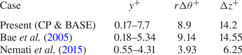
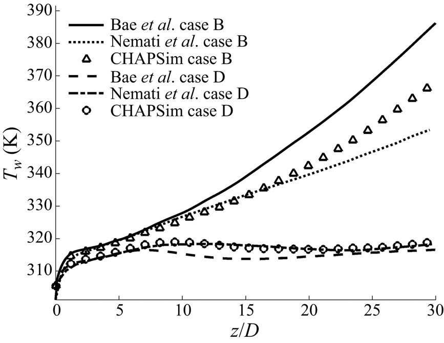
The computational domain of the heated pipe is 40 diameters long with an inflow and outflow boundary condition. A separate flow generator of 5 diameters in length is used to produce instantaneous turbulent inlet conditions of an isothermal flow and periodic boundary conditions are used at the inlet and outlet to produce a fully developed turbulent flow. The heated flow domain is discretised on a mesh of  $1024 \times 64 \times 128$ in the streamwise, radial and circumferential directions, respectively, with the flow generator using a mesh of
 $128 \times 64 \times 128$. The resulting non-dimensional spacing for the heated pipe is
 $\Delta z^{+}=14.2$,
 $\Delta y^+=0.17 \sim 7.7$ and
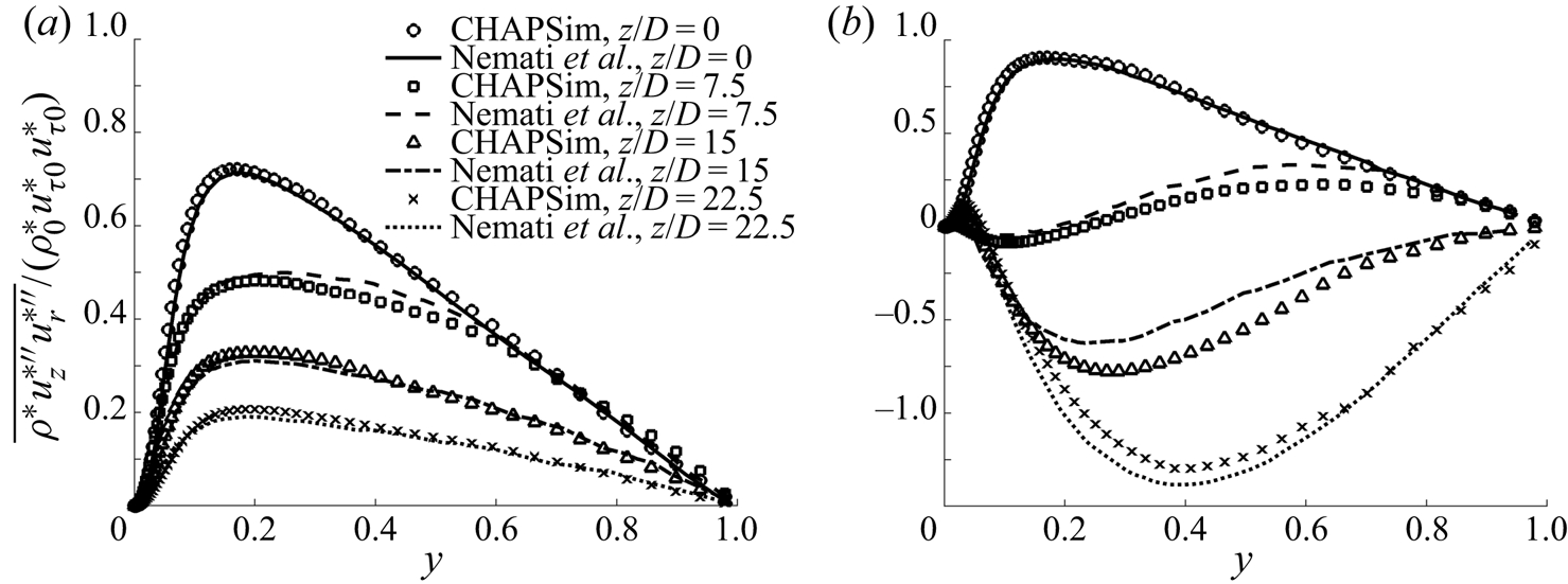
 $\Delta r \theta ^+ = 8.9$ based on the inflow condition. The suitability of the mesh used is discussed in Appendix A and further validation can also be found in He et al. (Reference He, Yan, Wang, Jiang and He2020).
In this paper, two types of average scheme are used: the Reynolds average with an overbar denoting the Reynolds-averaged value ( $\bar {\phi }$), and a single prime denoting the fluctuating component (
 $\phi '$); and the Favre average (density-weighted average), with a tilde denoting the averaged value (
 $\tilde {\phi }=\overline {\rho \phi }/\bar {\rho }$), a double prime denoting the fluctuating component (
 $\phi ''$) and
 $\phi = \bar {\phi }+\phi '$ and
 $\phi = \tilde {\phi }+\phi ''$. The average is performed circumferentially as well as over a period of time after the flow has reached a stationary state.
3. Results and discussion
3.1. General flow and turbulence characteristics
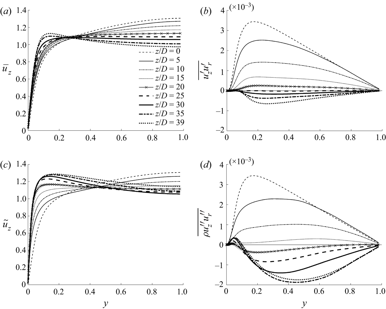
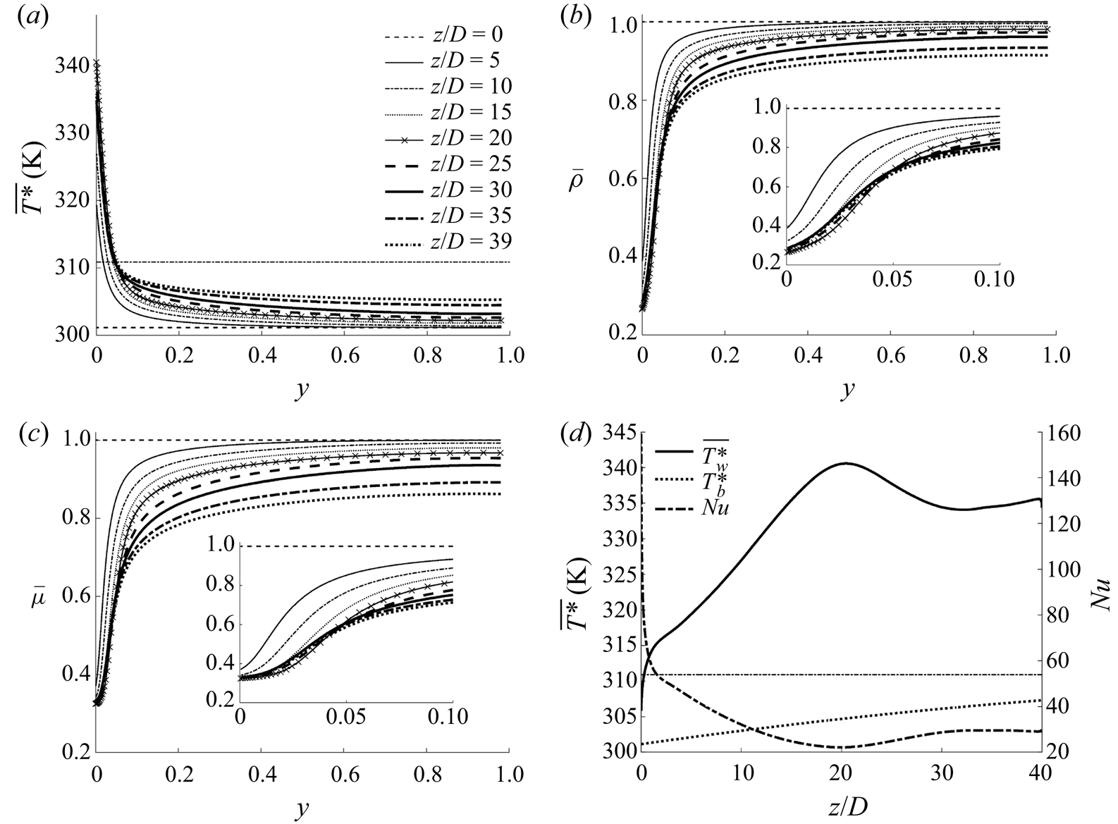
The general behaviour of the flow can be summarised with reference to figure 1, in which the developments of the radial profiles of the velocity and turbulent shear stress for cases CP and BASE are shown, and figure 2, in which the radial profiles of the density, viscosity and temperature and the axial developments of the bulk and wall temperatures and the Nusselt number in case BASE are shown. The two cases show qualitatively similar behaviour. As the fluid is heated in an upward flow, it becomes lighter near the wall, resulting in a buoyant force aiding the flow, which in turn causes the fluid in that region to accelerate relative to the fluid in the core, resulting in a flattened velocity profile. At a later stage, the near-wall fluid accelerates so much that the peak of the profile shifts away from the pipe centre to a location near the wall, and the velocity profile becomes so-called M-shaped. Correspondingly, the turbulent shear stress reduces downstream initially and reaches the lowest level (close to zero everywhere in the pipe) around the time when the velocity profile is about to switch its shape. Further downstream, turbulence is regenerated. In comparison with case CP, the turbulence in case BASE laminarises stronger and faster in the first stage, and then it recovers also stronger and faster in the later stages, clearly due to the effects of variations of thermophysical properties in addition to buoyancy. Heat transfer deterioration occurs around the location at which turbulence is minimised, where the Nusselt number is minimum and the wall temperature peaks (figure 2d).
Radial profiles of the mean velocity and turbulent shear stress at several streamwise locations in case CP in the form of Reynolds average (a,b) and case BASE in the form of Favre average (c,d).

Radial profiles of (a) the temperature, (b) density and (c) viscosity and (d) the axial developments of the bulk and wall temperatures and the Nusselt number in case BASE. The pseudo-critical temperature is marked using a dashed line.

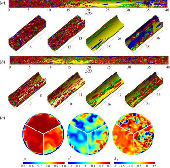
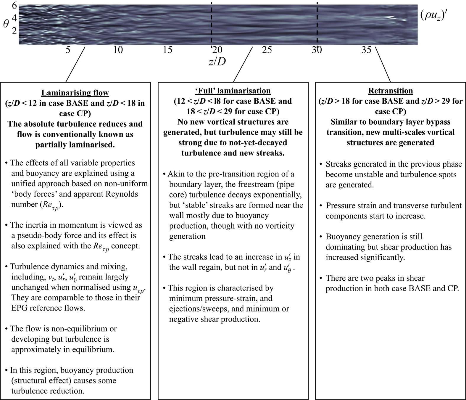
The phenomenon described above is well established and has been studied in various investigations (e.g. refer to review articles by Jackson Reference Jackson2013; Yoo Reference Yoo2013). Generally speaking, the flow and turbulence behaviours in such a heated supercritical fluid flow show a clear three-stage development, that is, a partially laminarising flow stage, a full laminarisation stage and a re-transition stage. Both turbulence and heat transfer exhibit distinct characteristics in each of the stages/regions. The developments of the turbulence structures along the pipe in both cases are illustrated in figure 3 using iso-surfaces of  $\pm u'$ for high- and low-speed streaks and
 $\lambda _2$ for vortical structures, where
 $\lambda _2$ is the second largest eigenvalue of a symmetric tensor formed using the velocity gradient to show the vortex cores (Jeong & Hussain Reference Jeong and Hussain1995). For case CP, both streaks and vortices reduce along the pipe first and have largely disappeared at approximately
 $z/D=18$, and remain so until
 $z/D=29$, after which turbulence is regenerated. The corresponding locations for case BASE are
 $z/D=12$ and
 $18$ respectively. In this study, the regions of
 $18< z/D<29$ and
 $12< z/D<18$ in cases CP and BASE, respectively, are referred to as the full laminarisation regions, which separate the laminarising and re-transition regions before and after it. There may still be strong turbulent kinetic energy in the region of full laminarisation referred to herein. The reasons for this and the particular categorisation of the flow regions and the boundaries between them (used above) will become clear later.
Turbulence structures. (a) Streaks and vortical structures in case CP ( $u_z '= \pm 0.12$ in green and blue respectively,
 $\lambda _2 = -0.15$ in red) and (b) in case BASE (
 $u_z '= \pm 0.19$,
 $\lambda _2 = -0.6$). Only half of the pipe is shown and the full-length pipe shown at the top is shrunk axially. (c) Instantaneous density, fluctuating velocity (
 $u_z '$) and
 $\lambda _2$ in case BASE at
 $z/D=4$ (top), 12 (left) and 35 (right).

We are interested in understanding the mechanisms of flow laminarisation, especially with respect to the apparent Reynolds number theory proposed in He et al. (Reference He, He and Seddighi2016). The theory is based on the effect of the non-uniform body forces, and to understand such forces in the flow we are concerned with, we analyse the momentum balances. Consider the integrated Favre-averaged streamwise momentum equation
 \begin{align} &-\frac{1}{r}\int^{r}_{0}r\frac{\partial(\bar{\rho} \tilde{u}_z\, \tilde{u}_z)}{\partial z}\,\textrm{d}r - \bar{\rho} \tilde{u}_z\, \tilde{u}_r -\frac{1}{r}\int^{r}_{0}r\frac{\partial(\overline{\rho u_z'' u_z''})}{\partial z}\,\textrm{d}r \vphantom{\int^{r}_{0}} - \overline{ \rho u_z'' u_r''}\nonumber\\ &\quad + \frac{1}{Re_0} \left( \frac{1}{r} \int^{r}_{0} r \frac{\partial}{\partial z}\left(2\bar{\mu}\frac{\partial \tilde{u}_z}{\partial r}\right)\textrm{d}r + \bar{\mu}\left(\frac{\partial \tilde{u}_r}{\partial z}+\frac{\partial \tilde{u}_z}{\partial r}\right) \right)\nonumber\\ &\quad - \frac{r}{2}\frac{\partial P}{\partial z} - \frac{1}{r} \frac{1}{Fr_0^2} \int_{0}^{r} r(\overline{\rho}-\overline{\rho}_c) \,\textrm{d}r = 0, \end{align}
where  $\rho _c$ is the density at the pipe centreline and
 ${\partial P}/{\partial z} \equiv ({\partial \bar {p}}/{\partial z}+ {\bar {\rho }_c}/{Fr_0^2})$ is the modified pressure gradient. From left to right, the equation includes, the inertial terms (
 $IN, \times 2$), turbulent shear stresses (
 $TS, \times 2$), the viscous shear stresses (
 $VS, \times 2$) and finally the (modified) pressure gradient (
 $PG$) and the buoyancy (
 $Bo$). It is worth noting that the first turbulent and viscous shear stress terms are both negligibly small and can be omitted without loss of accuracy. For case CP with the Boussinesq approximation, the Favre-averaged velocity and turbulent stresses are replaced by the Reynolds averages, and the normalised density and viscosity are both unity.
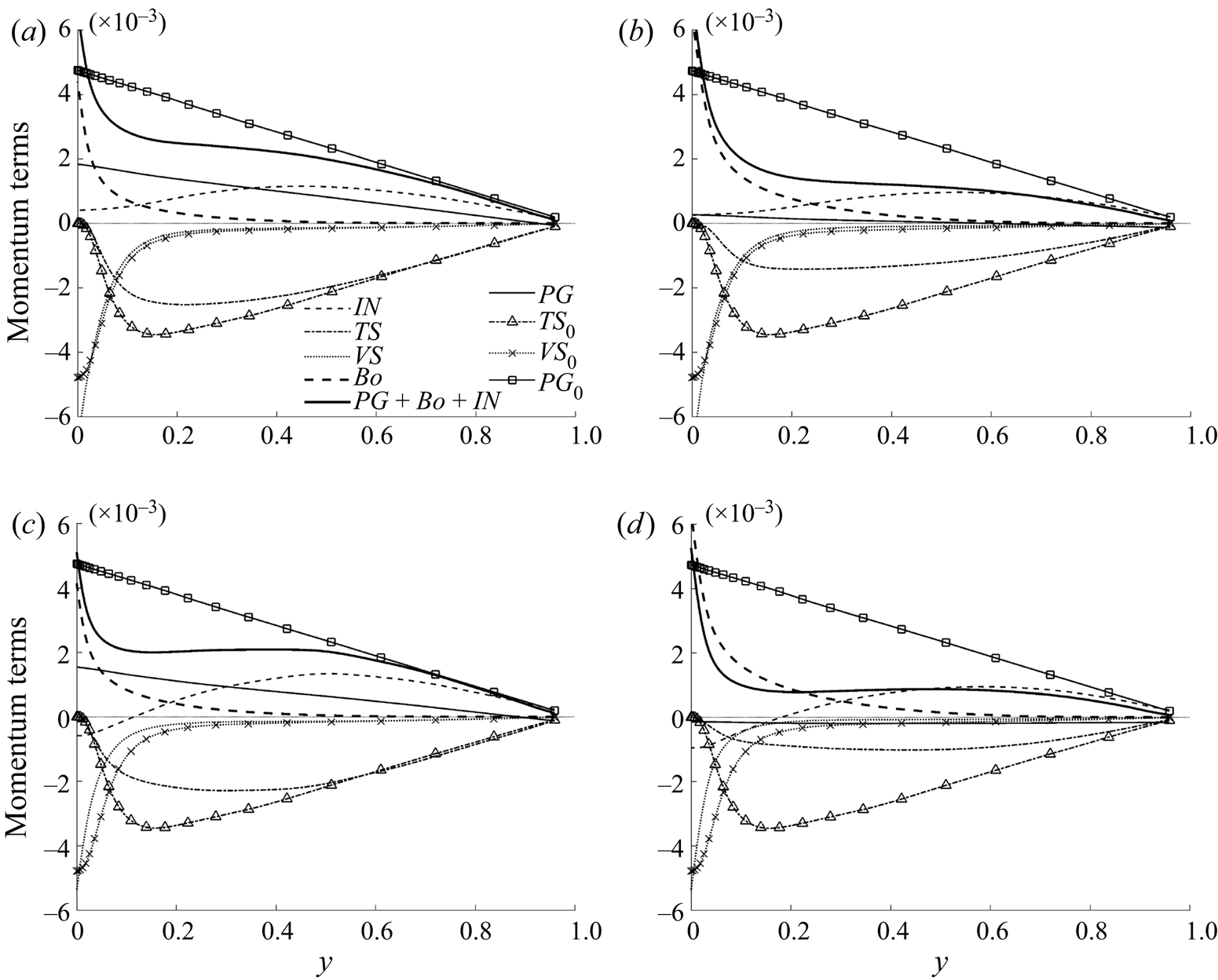
The momentum balances are shown in figure 4 for two locations in the laminarising region for cases CP and BASE. Considering case CP first, it is clear that the viscous shear stress remains largely unchanged at both  $z$-locations in comparison to the unheated flow, except very close to the wall where it is increased significantly. The turbulence shear reduces more strongly at
 $10D$ than at
 $5D$, as already observed in figure 1. The linearly distributed modified pressure force reduces strongly even at
 $5D$, and becomes close to zero at
 $10D$. The buoyancy is largely zero in most of the core of the pipe but increases sharply near the wall, being much larger at
 $10D$ than at
 $5D$. Finally, it is interesting to note that the inertia term is very strong in comparison with the other terms, and is largely linear in the pipe core, but reduces rapidly close to the wall. The general behaviour of the momentum balance in case BASE is similar to that in case CP, although the changes are generally faster and stronger for the same location. In particular, the viscous shear is significantly reduced in case BASE in a region near the wall.
Momentum balance (3.1) for case CP (top) and case BASE (bottom) at (a,c)  $z/D=5$ and (b,d)
 $z/D=10$. Those for an unheated flow are also shown for comparison. Every third data point is shown, with lines with markers for clarity.

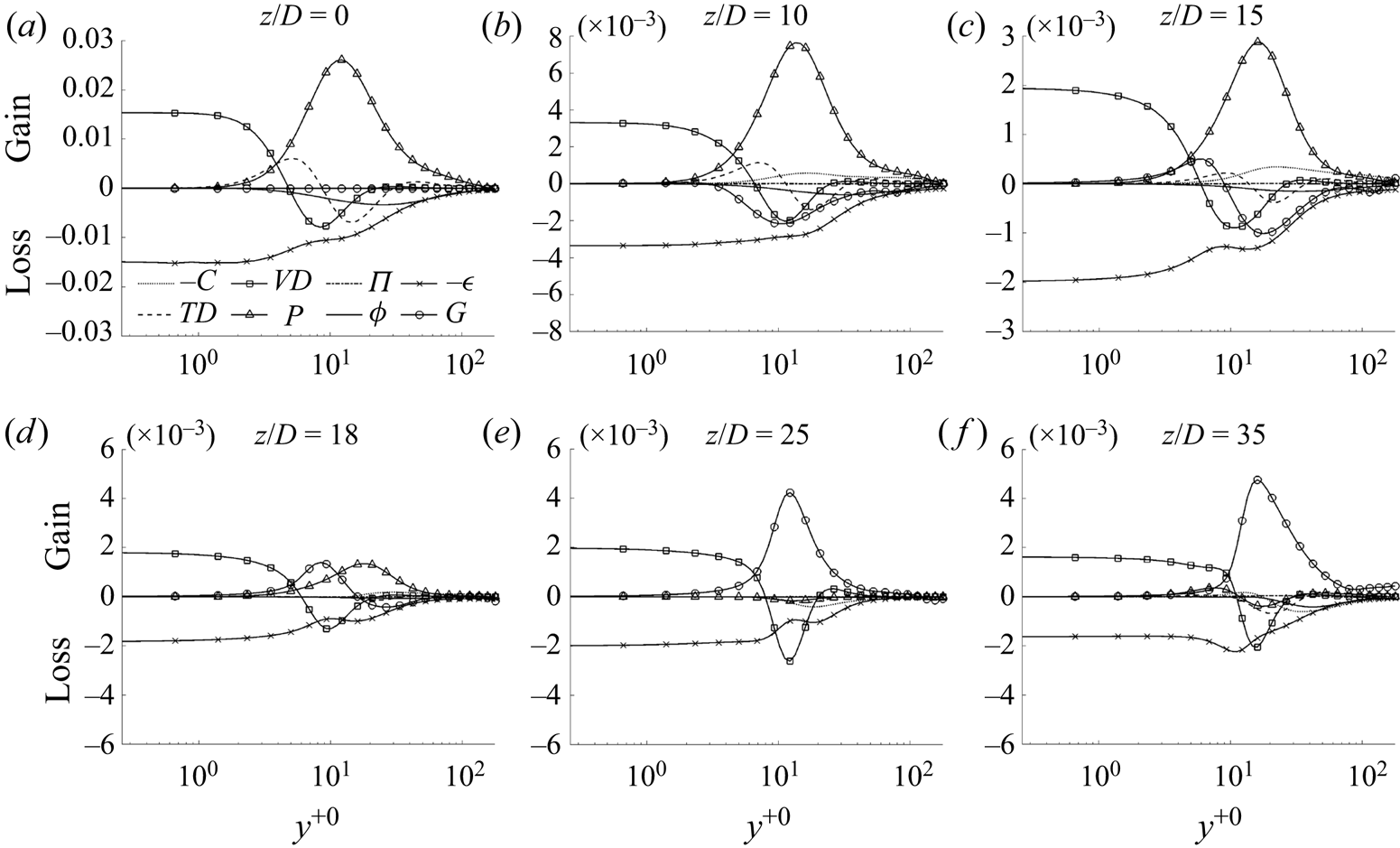
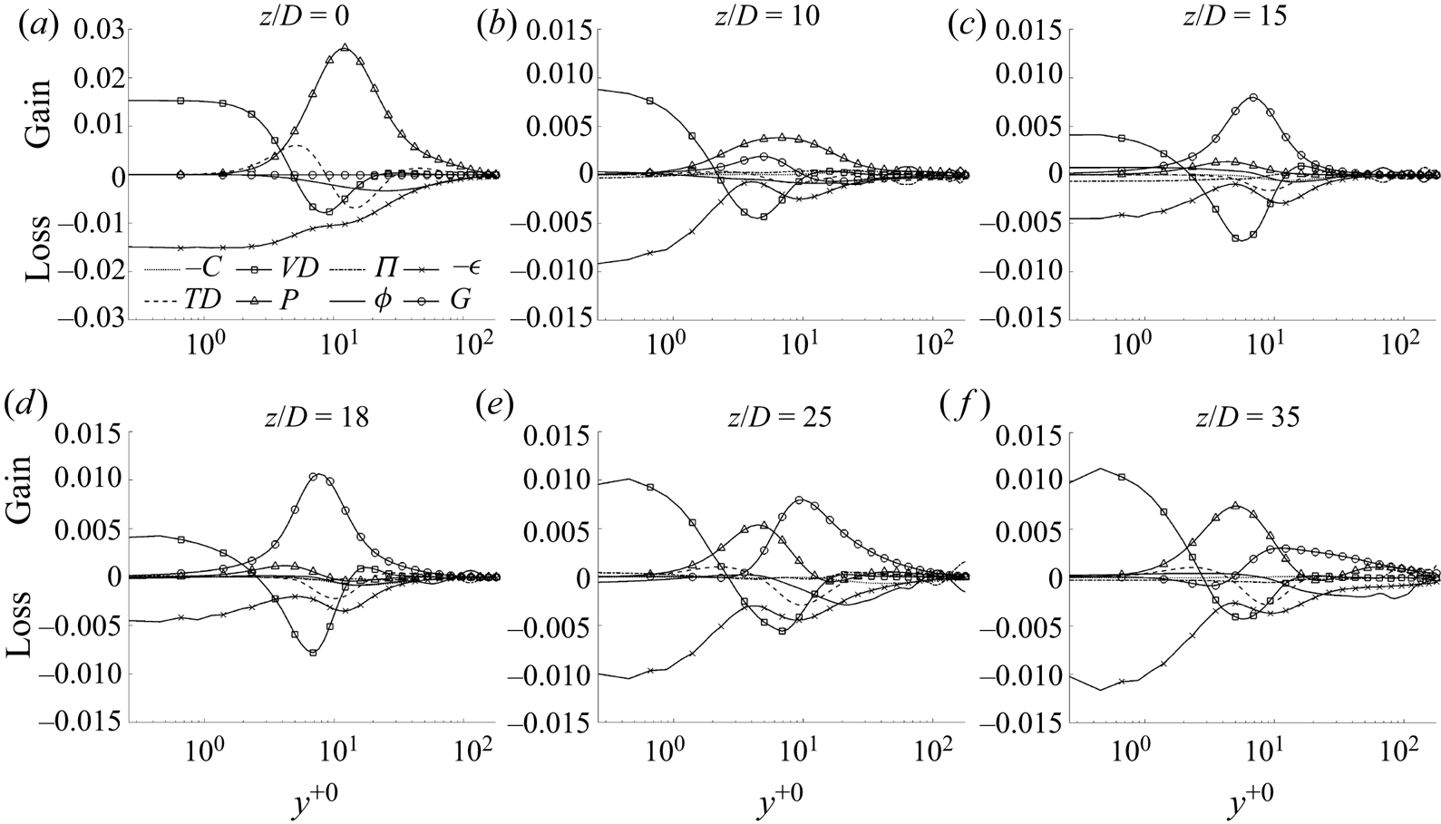
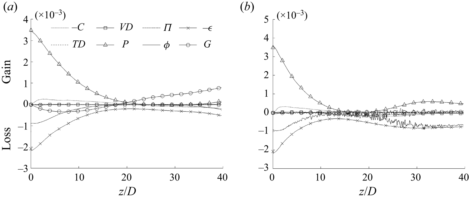
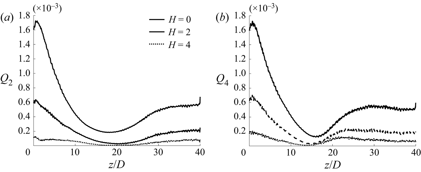
Before moving to the next section, we briefly discuss the budget of the streamwise turbulent stresses, which are shown in figures 5 and 6 for cases CP and BASE with, additionally, the cross-sectional integration in figure 7. The transport equation is given in Appendix B. First, it is interesting to note that the buoyancy production (structural effect) is negative but small in the laminarising region. Consequently, the turbulence dynamics is largely influenced by the indirect effects. The buoyancy production is, however, dominant in the full laminarisation and re-transition regions for both cases CP and BASE. Another point to note is that the convection makes only a small contribution to the overall turbulence budget balance in the flow laminarising region. This is both interesting and significant. Even though the inertia (spatial acceleration) plays a very significant part in the momentum balance in this developing flow, as shown above, the turbulence is, however, largely in equilibrium. That is, the production of turbulence is approximately equal to its dissipation at any cross-section and turbulence is only insignificantly influenced by the flow up- and downstream of it. This, together with the first point, the buoyancy production being small in the laminarising region, provides the foundation for the analysis provided in §§ 3.2 to 3.4, where it is implicitly assumed that the indirect buoyancy effect is dominant and that the turbulence is largely local equilibrium.
The budget of the transport equation for  $\overline {u'_{z} u'_{z} }$ in case CP. Every third data point is shown, with lines with markers for clarity. The budget terms are: convection (
 $C$), viscous diffusion (
 $VD$), pressure diffusion (
 $\varPi$), dissipation (
 $\epsilon$), turbulence diffusion (
 $TD$), production (
 $P$), pressure strain (
 $\varPhi$) and buoyancy production (
 $G$).

The budget of the transport equation for  $\overline {\rho u''_{z} u''_{z}}$ in case BASE. Every third data point is shown, with lines with markers for clarity.

The radial integration of the budget of the transport equation for (a)  $\overline {u'_{z} u'_{z} }$ in case CP and (b) for
 $\overline {\rho u''_{z} u''_{z}}$ in case BASE.

The rest of this section is arranged as follows: § 3.2 discusses the apparent Reynolds number concept introduced in He et al. (Reference He, He and Seddighi2016) and new hypotheses proposed to extend the theory to the flow concerned herein, the validity of which is evaluated in § 3.3. This is followed by the discussion of a new unified explanation for the various laminarisation mechanisms in § 3.4. These discussions (§§ 2 to 4) are mostly applicable to the partially laminarising region, whereas the ‘full’ laminarisation and re-transition are discussed in § 3.5.
3.2. Apparent Reynolds number and pseudo-body forces
He et al. (Reference He, He and Seddighi2016) studied a spatially fully developed flow subjected to a prescribed non-uniform body force varying linearly with radius or in a step change manner to approximate the buoyancy in a heated upward flow using DNS. Not surprisingly, it was found that the idealised body forces cause partial or full laminarisation in a similar manner as the buoyancy does. The intriguing new finding was that the main turbulence characteristics of the body-force influenced flow, including the turbulence mixing represented by the eddy viscosity, are similar to those in a flow with the same pressure gradient without the presence of the body force. This flow was referred to as the EPG reference flow. In other words, applying an additional non-uniform body force does not cause significant changes to the key turbulence characteristics.
Making use of the eddy-viscosity turbulence concept, the Reynolds-averaged momentum equation for such a spatially developed flow in a pipe with constant properties subject to a non-uniform body force ( $f$) can be written as
 \begin{equation} -\frac{\partial \bar{p}}{\partial z} + \frac{1}{r Re_0} \frac{\partial}{\partial r} \left(r(\nu_t +1) \frac{\partial \bar{u}_z}{\partial r}\right) + f = 0, \end{equation}
where  $\nu _t = \nu _t^*/\nu ^*$ is the non-dimensional eddy viscosity and the corresponding EPG reference flow is then
 \begin{equation} -\frac{\partial \bar{p}_p}{\partial z} + \frac{1}{r Re_0} \frac{\partial}{\partial r} \left(r(\nu_{tp} +1) \frac{\partial \bar{u}_{p} }{\partial r}\right) = 0, \end{equation}
where  ${\partial \bar {p}}/{\partial z}={\partial \bar {p}_p}/{\partial z}$ by the definition of EPG flow and the observation of He et al. (Reference He, He and Seddighi2016) outlined above implies that
 $\nu _t = \nu _{tp}$. Subtracting (3.3) from (3.2), we have
 \begin{equation} \frac{1}{r Re_0} \frac{\partial}{\partial r} \left(r(\nu_{tp} +1) \frac{\partial \bar{u}_f }{\partial r}\right) + f = 0, \end{equation}
where  $\bar {u}_f= \bar {u}_z -\bar {u}_{p}$, which is a perturbation caused by the body force. Consequently, the body-force influenced flow can be represented by the EPG flow plus the body-force induced perturbation flow. The authors then defined an apparent friction velocity for the flow based on the pressure gradient,
 $u^*_{\tau p}=\sqrt {\tau ^*_{wp}/\rho ^*}$, where
 $\tau ^*_{wp}=-(R^*/2)(\partial \bar {p}^* /\partial z^*)$. Similarly, an apparent Reynolds number can be defined as
 $Re_{\tau p} = u^*_{\tau p} R^*/\nu ^*$. It follows naturally from the observation described above that the flow statistics of a body-force influenced flow, when normalised by the apparent friction velocity, would behave in a similar manner as those in the EPG flow, which was demonstrated by He et al. (Reference He, He and Seddighi2016). The turbulence reduction, or the so-called laminarisation, commonly referred to when compared with a reference flow of the same flow rate, can then be associated with a reduction in the Reynolds number of the EPG flow (i.e. the
 $Re_{\tau p}$).
The principal hypothesis of this paper is that, for the various flow laminarising mechanisms in a heated flow including the buoyancy, the variations of thermophysical properties and even the inertia can be explained with the apparent Reynolds number (ARN) theory.
We first consider the variations of density and viscosity. For this purpose, we consider a stationary, streamwise fully developed flow with non-uniform density and viscosity distributions but without the effect of gravity. An example of this is the flow in parallel plates with a heated and a cooled wall on either side, as studied by Peeters et al. (Reference Peeters, Pecnik, Rohde, Van Der Hagen and Boersma2016) and Wan et al. (Reference Wan, Zhao, Liu, Wang and Lei2020). The governing equation for the mean flow based on the Favre average reads
 \begin{equation} -\frac{\partial \bar{p}}{\partial z} + \frac{1}{r Re_0} \frac{\partial }{\partial r} \left( r \left({-}Re_0 \overline{\rho u''_{z} u''_{r}} + \bar{\mu} \frac{\partial \tilde{u}_z}{\partial r} \right) \right) = 0, \end{equation}
which can be re-written as follows after introducing the eddy-viscosity modelling concept,  $-\overline {\rho u''_{z} u''_{r}}/\bar {\rho }= ({\nu _t}/{Re_0}) ({\partial \tilde {u}_z}/{\partial r})$:
 \begin{equation} -\frac{\partial \bar{p}}{\partial z} + \frac{1}{r Re_0} \frac{\partial}{\partial r} \left(r(\bar{\rho} \nu_t + \bar{\mu}) \frac{\partial \tilde{u}_z}{\partial r}\right)=0. \end{equation}
Consider a new flow with an equivalent pressure gradient, but with a uniform and constant density and viscosity distribution,
 \begin{equation} -\frac{\partial \bar{p}_p}{\partial z} + \frac{1}{r Re_0} \frac{\partial}{\partial r} \left(r(\rho_p \nu_{tp} + \mu_p) \frac{\partial \bar{u}_{p} }{\partial r}\right)=0, \end{equation}
where  $-\partial \bar {p}_p/\partial z = -\partial \bar {p}/\partial z$ and the subscript ‘
 $p$’ refers to the reference flow condition, which is taken as that at the centreline here. As discussed in the Introduction, the density and viscosity variations have been found to have negligible influence on the turbulence dynamics in various previous studies, and this knowledge has been used in a number of studies as a basis for flow and turbulence scaling (Huang et al. Reference Huang, Coleman and Bradshaw1995; Patel et al. Reference Patel, Boersma and Pecnik2016; Trettel & Larsson Reference Trettel and Larsson2016). The ‘unchanged turbulence dynamics’, however, can be interpreted in different ways. In the original van Driest analysis for cases where only internal frictional heating was considered, this was taken to mean that the mixing length is an invariant in constant and variable density flows. When more complex (heating) conditions are considered in more recent studies (which may involve variations of density and viscosity), additional scaling has been found necessary, including for example the use of the semi-local parameters and a new local Reynolds number (
 $Re_\tau ^*$). Here, we follow the analysis of He et al. (Reference He, He and Seddighi2016), assuming the eddy viscosity in the heated flow and its equivalent reference flow are the same, that is,
 $\nu _t=\nu _{tp}$. Now, subtracting (3.7) from (3.6),
 \begin{equation} \frac{1}{r Re_0} \frac{\partial}{\partial r} \left(r(\bar{\rho} \nu_{tp} + \bar{\mu}) \frac{\partial \bar{u}_f}{\partial r}\right) + \frac{1}{r Re_0} \frac{\partial}{\partial r} \left(r ( (\bar{\rho}-\rho_p) \nu_{tp}+(\bar{\mu}-\mu_p) ) \frac{\partial \bar{u}_{p} }{\partial r}\right)=0, \end{equation}
where  $\bar {u}_f = \tilde {u}_z - \bar {u}_p$. It is useful to note that, in the context of this analysis, the Reynolds- and Favre-averaged mean velocities are very close, even under strong heating, that is
 $\tilde {u}_z \simeq \bar {u}_z$. A direct comparison between the two mean velocities is given in the next section and discussions can also be found in Huang et al. (Reference Huang, Coleman and Bradshaw1995) and Ma et al. (Reference Ma, Yang and Ihme2018). The above equation can be re-written with the effects of density and viscosity separated,
 \begin{equation} \frac{1}{r Re_0} \frac{\partial}{\partial r} \left(r(\bar{\rho} \nu_{tp} + \bar{\mu}) \frac{\partial \bar{u}_{f} }{\partial r}\right)+f_{1b}+ f_{1c}=0, \end{equation}
where
 \begin{equation} f_{1b} = \frac{1}{r Re_0} \frac{\partial}{\partial r} \left(r (\bar{\mu} - \mu_p) \frac{\partial \bar{u}_{p} }{\partial r}\right) \end{equation}
and
 \begin{equation} f_{1c} = \frac{1}{r Re_0} \frac{\partial}{\partial r} \left(r (\bar{\rho}-\rho_p) \nu_{tp} \frac{\partial \bar{u}_{p} }{\partial r}\right). \end{equation}
We refer to  $f_{1b}$ and
 $f_{1c}$ as the pseudo-body forces due to viscosity and density variations, respectively. They cause a perturbation flow
 $\bar {u}_f$ on top of the base (EPG) flow
 $\bar {u}_{p}$. Like the body-force influenced flow in He et al. (Reference He, He and Seddighi2016), the heated flow with variable properties can be represented by a constant-property EPG flow plus a perturbation flow. Furthermore, the latter (perturbation) is only a function of the non-uniform distributions of the density and viscosity, and the eddy viscosity of the EPG flow. In fact, (3.9) can be rearranged to obtain an explicit expression for the velocity gradient of the perturbation flow as
 \begin{equation} \frac{\partial \bar{u}_{f} }{\partial r} = \left(\frac{(\bar{\rho}-\rho_p)\nu_{tp} + (\bar{\mu}-\mu_p)}{\bar{\rho} \nu_{tp}+\bar{\mu}} \right) \frac{\partial \bar{u}_{p} }{\partial r}. \end{equation}
For a general case, such as case BASE, the flow is also complicated by the spatial development. For the flow away from the immediate start of the heating (say  $z/D>1$), the terms of minor contribution can be neglected (as for the boundary layer equations) and the Favre-averaged streamwise momentum can be written as
 \begin{equation} -\frac{\partial (\bar{\rho} \tilde{u}_z \tilde{u}_z)}{\partial z} - \frac{1}{r} \frac{\partial (r \bar{\rho} \tilde{u}_r \tilde{u}_z)}{\partial r} -\frac{\partial \bar{p}}{\partial z} + \frac{1}{r Re_0} \frac{\partial}{\partial r} \left(r\left({-}Re_0 \overline{\rho u''_z u''_r} + \bar{\mu} \frac{\partial \tilde{u}_z}{\partial r}\right)\right)-\frac{\bar{\rho}}{Fr_0^2}=0. \end{equation}
As shown in figure 4, the inertia is very significant in the developing flow we are concerned with, strongly influencing the flow dynamics. Here, we make a proposition that the inertia can be treated as a pseudo-body force, acting on the flow in a similar way as the buoyancy, and that it does not cause the turbulence to change when compared with that of the EPG flow. Under this assumption, we can then group it together with other body forces (pressure and buoyancy) to form the total body force for the flow. As for gravity, the inertia can be split into a uniform and a non-uniform component, with the uniform component taken to be the value at the pipe centreline. The total inertial force  $f_{2}$, its uniform
 $f_{2U}$ and non-uniform
 $f_{2N}$ components are then
 \begin{equation} f_{2}={-}\frac{\partial(\bar{\rho} \tilde{u}_z \tilde{u}_z)}{\partial z} - \frac{1}{r} \frac{\partial (r \bar{\rho} \tilde{u}_r \tilde{u}_z)}{\partial r}, \end{equation}
and
 \begin{equation} f_{2U}= f_2(r=0) \quad \text{and}\quad f_{2N}=f_2 - f_2(r=0). \end{equation}
The proposition for the linear component is clearly true as, physically, this implies that the fluid in the entire cross-section accelerates as a solid body in response to a uniform body force (pressure or otherwise), without modifying the relative flow (i.e. the strain field). The success of the proposition regarding the non-uniform component and the applicability of the overall non-uniform body-force effect proposed in He et al. (Reference He, He and Seddighi2016) to the flow concerned herein are evaluated in the next section.
Considering all the above analyses together, the heated flow can now be represented by the sum of the EPG flow and a perturbation due to the total body force, which are described by the following equations, respectively:
 \begin{equation} -\left( \frac{\partial P}{\partial z} \right)_p + \frac{1}{r Re_0} \frac{\partial}{\partial r} \left(r(\rho_p \nu_{tp} + \mu_p) \frac{\partial \bar{u}_{p}}{\partial r}\right)=0, \end{equation}
and
 \begin{equation} \frac{1}{rRe_0} \frac{\partial}{\partial r} \left(r(\bar{\rho} \nu_{tp} + \bar{\mu}) \frac{\partial \bar{u}_f}{\partial r}\right)+f_{T}=0, \end{equation}
where the total modified pressure gradient is
 \begin{equation} -\left( \frac{\partial P}{\partial z} \right)_p ={-}\frac{\partial \bar{p}}{\partial z} - \frac{\bar{\rho}_p }{Fr_0^2} + f_{2U} \end{equation}
and the total non-uniform body force is
 \begin{equation} f_{T} = f_{1a} + f_{1b} + f_{1c} + f_{2N}, \end{equation}
where the buoyancy force (noting  $\bar {\rho }_p = \bar {\rho }_c$) is
 \begin{equation} f_{1a}={-}(\bar{\rho}-\bar{\rho}_c)/Fr_0^2 \end{equation}
and the non-uniform pseudo-body forces are given in (3.10), (3.11) and (3.15a,b). Under the assumptions introduced herein, for any location in the laminarising region of a heated flow, the turbulence dynamics can be approximated by that of the EPG flow (3.15a,b), the driving force of which is the total modified pressure gradient (3.18). On top of the EPG flow, a perturbation is caused by the combined action of the non-uniform (pseudo-)body forces (3.19), and the total mean flow is  $\tilde {u}_z = \bar {u}_p + \bar {u}_f$. In the following section, we evaluate the assumptions introduced above against cases CP and BASE.
3.3. Evaluation of the apparent Reynolds number (ARN) analysis of flow laminarisation
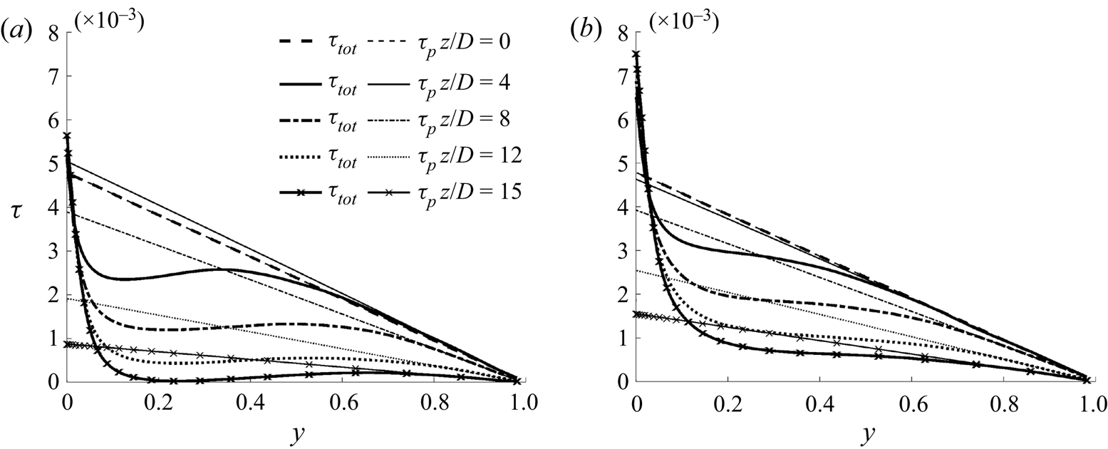
The profiles of the total shear stress together with their linear components (due to the total modified pressure gradient) in the laminarising region of cases CP and BASE are shown in figure 8. The total stress can also be computed from the total apparent body force,  $\tau _{tot} = -(r/2) ( \partial P / \partial z )_p + (1/r) \int _0^r rf_T \,\textrm {d}r$. The first term is the linear component (noted as
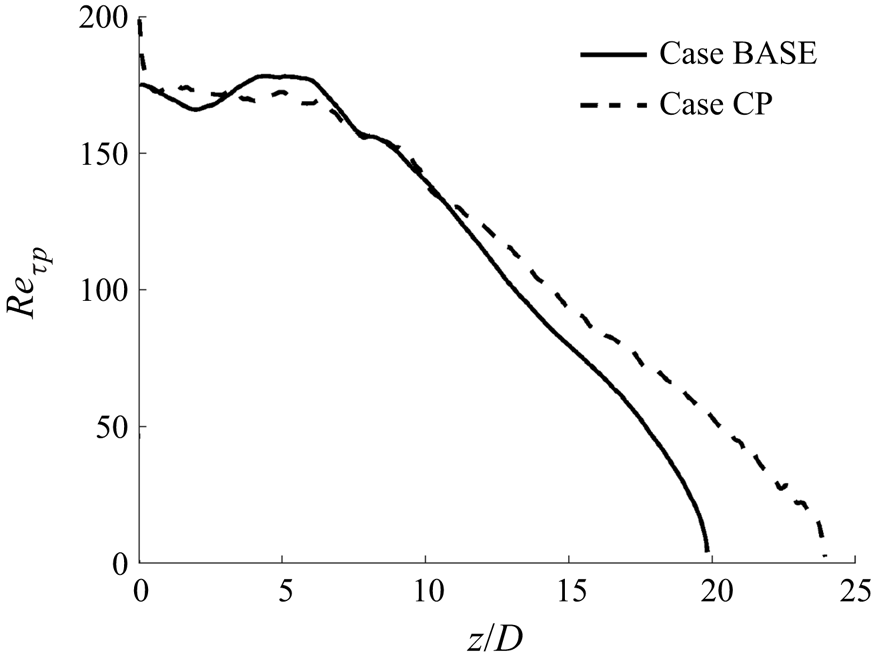
 $\tau _p$), which is used to define the ARN shown in figure 9. It is clear that, initially (
 $z/D<5$), the ARN (
 $Re_{\tau p}$) appears to remain largely unchanged, and then it reduces roughly linearly, faster in case BASE than in case CP. The
 $Re_{\tau p}$ reaches approximately 60 at approximately
 $z/D = 19$ and
 $17$ in cases CP and BASE, where the low Reynolds number would suggest that the flow would approach a laminar state for an equivalent unheated flow.
The shear stress due to the total (pseudo-)body force ( $\tau _{tot}$) and its linear component (
 $\tau _p$) in (a) case CP and (b) case BASE.

The ARN in cases CP and BASE.

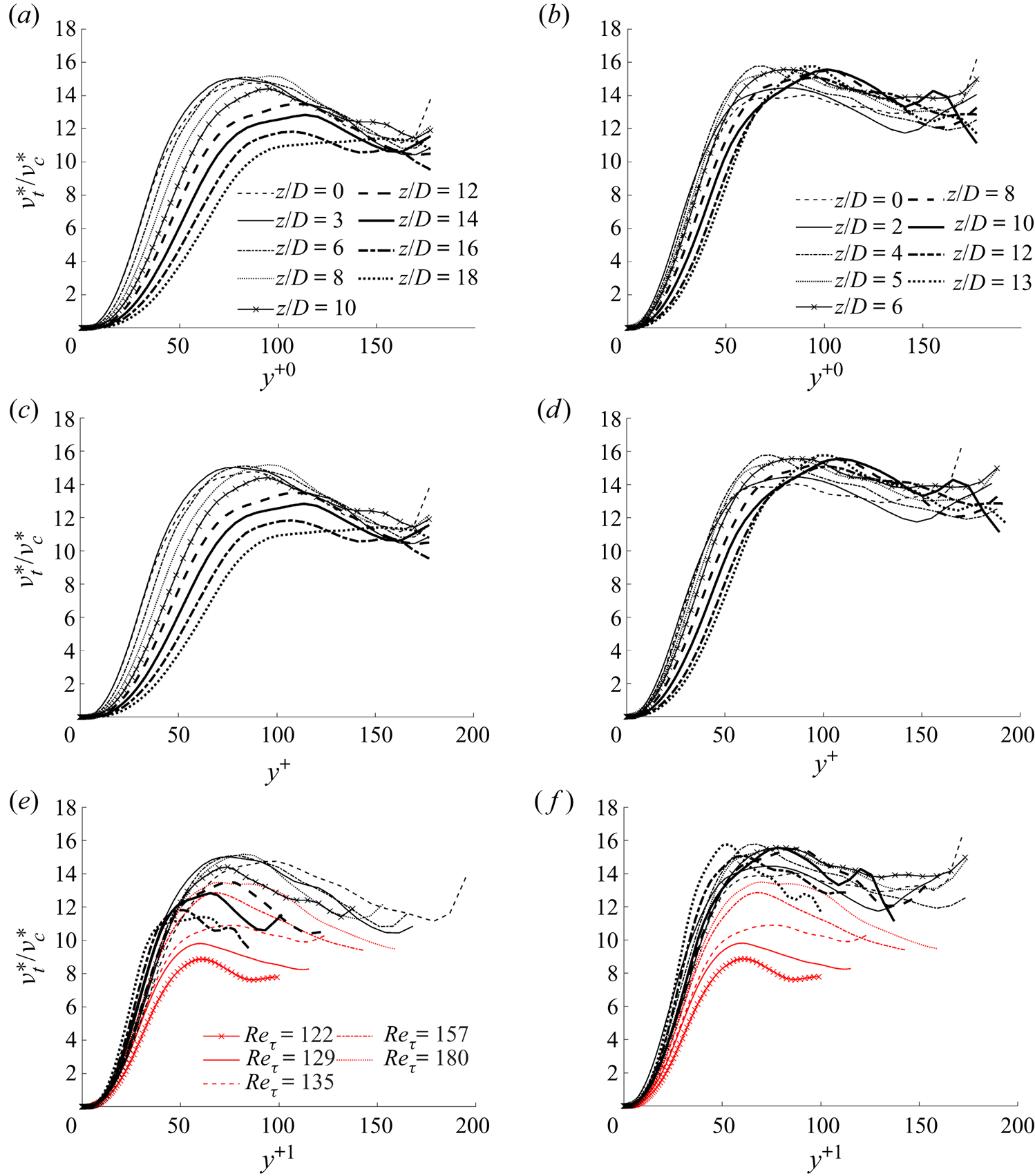
We first inspect the behaviour of the eddy viscosity to evaluate the applicability of the ARN theory. The distribution of the eddy viscosity in cases CP and BASE are shown in figure 10 against wall unit distance based on three different friction velocity definitions, that is, those based on the unheated flow ( $y^{+0}=\bar {\rho }^*_0 y^* u^*_{\tau 0}/{\bar {\mu }}^*_0$), the local wall shear stress (
 $y^{+}=\bar {\rho }^*_c y^* u^*_\tau /{\bar {\mu }}^*_c$) and the apparent wall shear stress (
 $y^{+1}=\bar {\rho }^*_c y^* u^*_{\tau p}/{\bar {\mu }}^*_c$). Here,
 $u^*_{\tau 0} = \sqrt {\tau ^*_{w0}/\bar {\rho }^*_0}$,
 $u^*_{\tau } = \sqrt {\tau ^*_w/\bar {\rho }^*_c}$ and
 $u^*_{\tau p}=\sqrt {\tau ^*_{wp}/\bar {\rho }^*}$, where
 $\tau ^*_{wp}=-(1/2)(\partial P^* /\partial z^*)_p$. The first normalisation shows the absolute changes in eddy viscosity with downstream distance, whereas the second normalisation shows how far the distributions deviate from that of the ‘universal’ distribution of an unheated flow; and finally the last normalisation would behave in a similar way as that in its corresponding unheated EPG reference flow if the ARN theory applies.
Eddy viscosity in cases CP (a,c,e) and BASE (b,d,f) plotted against various wall units.

It can be seen from figure 10(a,b) that the eddy viscosity at any fixed radial location in both cases CP and BASE reduces drastically streamwise in the wall region. For example, at  $y^{+0}=30$, it reduces from 5.7 to 0.9 in case CP and from 6.8 to 3.0 in case BASE. The change is small beyond
 $y^{+0}=60$ in case BASE, but significant reduction occurs until around
 $y^{+0}=100$ in case CP. The behaviour of
 $\nu _t (=\nu ^* _t / \nu ^* _c )$ vs
 $y^+$ is largely the same as that described above, although quantitatively the changes are marginally larger due to the increase of the wall shear stresses in the heated pipe. These observations are consistent with the conventional theory regarding flow laminarisation. The results also show that the flow in the core is less influenced, but the eddy viscosity is of more significance close to the wall where the velocity gradients are larger and the mixing effect due to turbulence is more significant.
In strong contrast, figure 10(e,f) shows that  $\nu _t$ does not reduce in the relaminarising region in both cases CP and BASE when plotted against
 $y^{+1}$. In fact, towards the end of the laminarising region, it starts to increase slightly. In such low Reynolds number flows, we normally expect that
 $\nu _t$ has some dependence on Reynolds number. To aid discussion, the
 $\nu _t$ in several flows of low
 $Re_\tau$ are shown for comparison. It can be seen that
 $\nu _t$ reduces with reducing Reynolds number in the core of the flow, although it is largely the same close to the wall, except for the lowest Reynolds number, where notable reduction is seen everywhere. Close to the wall, the general behaviour of
 $\nu _t$ in both cases is close to that of the reference flows, although deviations are clearly seen towards the late stage of the laminarising region due to the increase in
 $\nu _t$ discussed above. In the core,
 $\nu _t$ reduces significantly in case CP but not as much as that in the reference cases, whereas in case BASE,
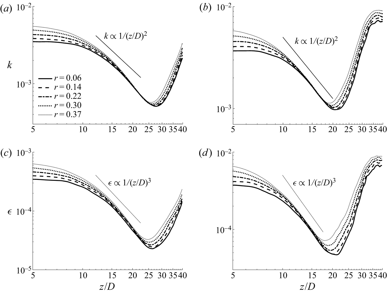
 $\nu _t$ hardly shows any reduction. This higher eddy viscosity reflects the presence of relatively stronger turbulence in the core of the flow and is likely due to an additional gain from the convection of turbulence from upstream. Since this largely occurs in the core of the flow, it does not have a significant influence on the overall flow dynamics, as demonstrated below.
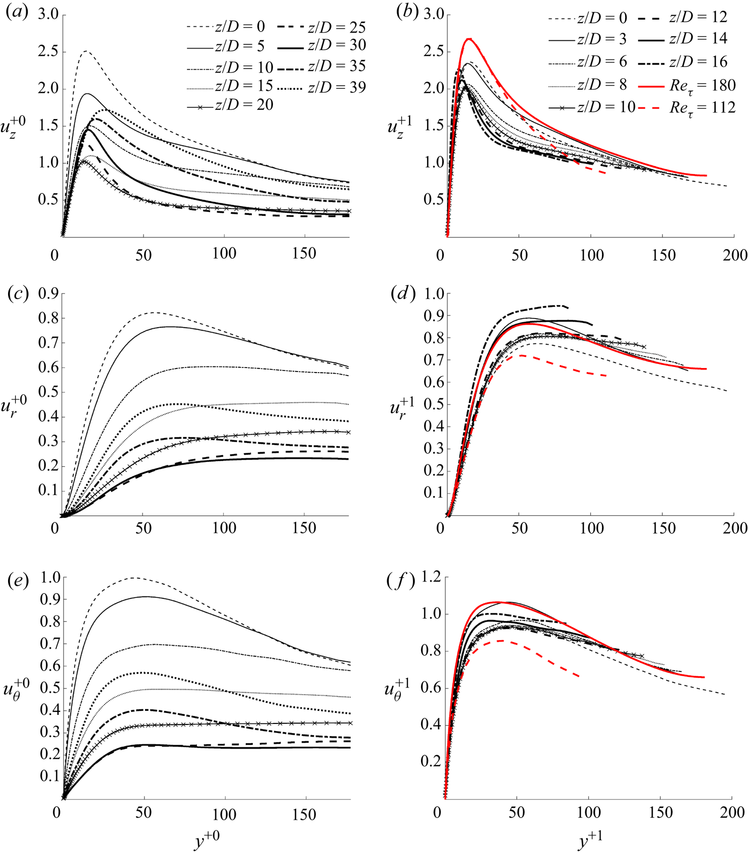
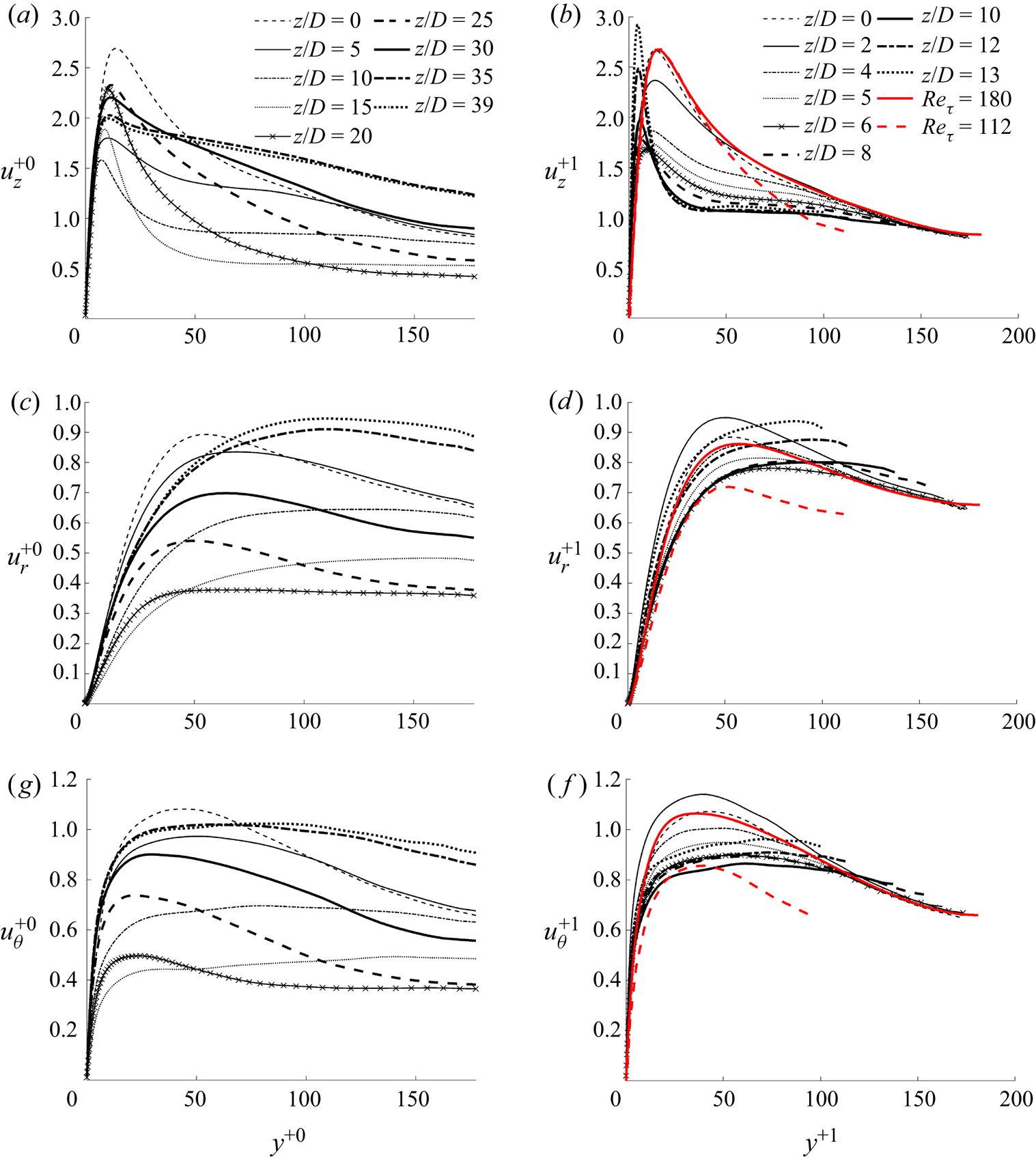
The r.m.s. of the turbulent fluctuating velocities non-dimensionalised using the  $u^*_{\tau 0}$ and
 $u^*_{\tau p}$ are shown in figures 11 and 12 for cases CP and BASE, respectively. The results normalised with
 $u^*_{\tau 0}$ are presented for locations over the full pipe length simulated, whereas those normalised by
 $u^*_{\tau p}$ are only shown up to the end of the laminarising region, where the ARN theory is to be evaluated. It is clear that the normal Reynolds stresses based on the former normalisation reduce significantly in the laminarising region in both cases, albeit stronger in case CP than in case BASE. The reduction is stronger in the normal and circumferential components than in the streamwise component. For example, the peaks of
 $u_z^{+0}$,
 $u_r^{+0}$ and
 $u_\theta ^{+0}$ reduce by approximately 60 %, 72 % and 76 %, respectively, in case CP, but 41 %, 58 % and 61 % in case BASE. When normalised using the local
 $u^*_\tau$ (not shown), the turbulence reduction is even stronger due to the increase of the wall shear stress in the heated pipe. These results demonstrate that the Reynolds stresses significantly reduce in both absolute terms and when normalised using the wall units as observed in many previous studies (e.g. Bae et al. Reference Bae, Yoo and Choi2005; Peeters et al. Reference Peeters, Pecnik, Rohde, Van Der Hagen and Boersma2016).
The r.m.s. fluctuating velocities in case CP normalised using the initial flow friction (left) and the apparent friction velocities (right). The latter are shown for only the partially laminarising region.

The r.m.s. fluctuating velocities in case BASE normalised using the initial flow friction (left) and the apparent friction velocities (right). The latter are shown for only the partially laminarising region.

We now inspect the r.m.s. fluctuating velocities normalised by the apparent wall shear stress and consider case CP first. It is known that the normal and circumferential stresses reduce slightly with reducing Reynolds number in low Reynolds number flows, but the streamwise component is largely Reynolds number independent. To capture such changes, the profiles for unheated flows at  $Re_\tau =112$ and
 $180$ are shown for comparison. It can be seen from the figure that
 $u_r^{+1}$ and
 $u_\theta ^{+1}$ fluctuate mostly within the bounds of the profiles of the two reference cases, and the changes are within
 $20\,\%$. This is in stark comparison with the drastic reductions observed when normalised by
 $u^*_{\tau 0}$ and
 $u^*_{\tau }$ discussed above. This finding is in accordance with the findings of He et al. (Reference He, He and Seddighi2016), and demonstrates that the two transverse normal stresses normalised by
 $u^*_{\tau p}$ based on the total modified pressure gradient can be reasonably well represented by those of their corresponding EPG flows. This observation, together with the behaviour of
 $\nu _t$ discussed above, provides evidence supporting the hypothesis that the strongly laminarised flows studied herein can be described by the reduction of the ARN and that the various factors, including variable properties and inertia, appear to act in a similar manner, in the form of (pseudo-)body forces, which are accounted for by the apparent friction velocity.
The behaviour of the streamwise component is, however, different. It reduces with downstream distance even though the peak of the reference results remains unchanged. This trend is opposite to that observed in He et al. (Reference He, He and Seddighi2016), in which the streamwise stress is higher than that in the corresponding EPG flow, which was attributed to the generation of streaks. The different behaviours can be attributed to the effect of the inertia, which is present in the developing flow we are concerned with here but not in He et al. (Reference He, He and Seddighi2016). As discussed later in § 3.3, the effect of inertia is opposite to other effects, reshaping the profile of the non-uniform body forces.
Next, we directly evaluate the key statement of the ARN theory, that is, the total flow can be represented by the EPG base flow plus a perturbation induced by the pseudo-body forces, and the latter does not cause any changes to the eddy viscosity. For the flow at any location in the laminarising region we are concerned with here, we can obtain the EPG via (3.18), and hence the ARN, which stipulates the EPG flow. Noting that such flows are ‘standard’ unheated pipe flow, the mean velocity and turbulence statistics of the flow (including the eddy viscosity) can be found from any database available. In addition, the total pseudo-body forces can be calculated (3.19) and then the perturbation velocity be estimated via (3.17). This then enables the total velocity profile to be calculated by simply summing the velocity of the EPG flow and the perturbation velocity. Additionally, the perturbation flow induces an additional turbulent shear stress as implied by (3.17), which can be computed as  $-(\overline {u'_{z} u'_{r}})_f =({\nu _{tp}}/{Re_0}) ({\partial \bar {u}_f}/{\partial r})$. The total shear stress in the heated flow is then the sum of this and that of the EPG flow.
The procedure described above implies that the only information required to ‘predict’ the mean velocity and turbulent shear stress is the eddy viscosity of the EPG flow with known  $(\partial P/\partial z)_p$ and
 $f_T$ of the laminarising flow. Herein, the eddy viscosity of unheated reference flow is obtained by interpolation using the data from He et al. (Reference He, He and Seddighi2016) for flows at
 $Re_\tau$ between 110 and 180. The EPG and the perturbation velocities are calculated by integrating twice (3.16) and (3.17), respectively. The corresponding turbulent shear stresses are then computed from
 $\nu _{tp}$ and the two velocity profiles.
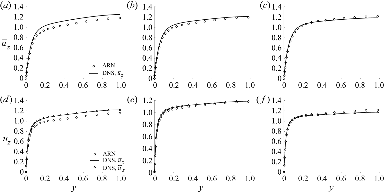
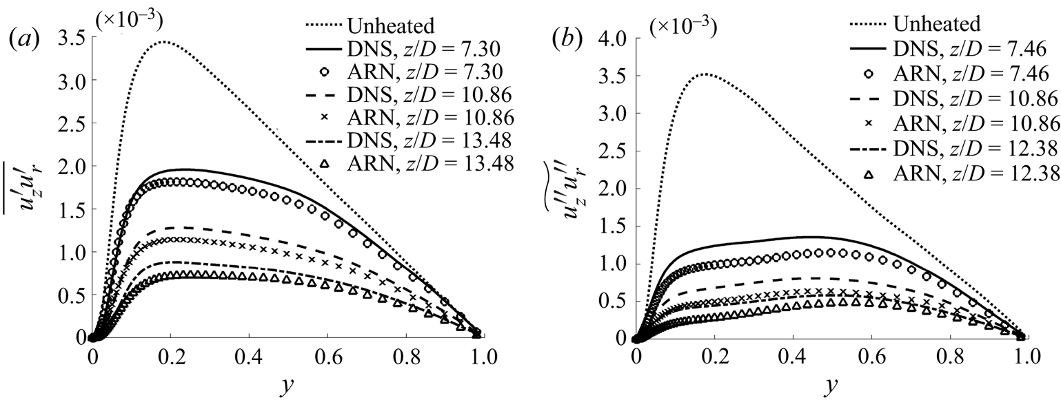
The mean velocity profiles and the turbulent shear stresses calculated using the ARN theory are compared to the DNS data in figures 13 and 14. It can be seen that the mean velocity of the DNS can be very well represented by the ARN theory at the later locations in both cases CP and BASE. Larger but still acceptable discrepancies are seen at the earlier position in both cases. In addition, it is seen that the Reynolds- and the Favre-averaged mean velocities in case BASE are practically indistinguishable, which is used in the analysis in the previous section. The ARN prediction of the turbulent shear stress for case CP agrees very well with the DNS with slightly larger discrepancies away from the wall and the pipe centre. The predictions for case BASE show larger discrepancies than for case CP, although the strong laminarisation has also been well captured. Overall, we consider these results demonstrate that the ARN theory is able to capture the general flow behaviour and laminarisation. It should be noted, however, that the above exercise does not really provide a full prediction of the heated flow, since it uses the thermophysical property distributions and the inertial terms from the DNS. It, however, provides new insights into the effects of the various factors on the turbulence dynamics and flow laminarisation. It is possible to utilise such new understanding in the future to improve modelling strategies, for example, following the work by Pecnik & Patel (Reference Pecnik and Patel2017).
Mean velocity in cases CP and BASE. Comparison between the DNS results and the ARN theory predictions at  $z/D = 7.30$, 10.86 and 13.48 in case CP (a–c) and 7.46, 10.86 and 12.38 in case BASE (d–f).

The turbulent shear stress in (a) case CP and (b) case BASE – comparison between the DNS results and ARN theory predictions.

3.4. A unified explanation for the laminarisation mechanisms in a heated pipe
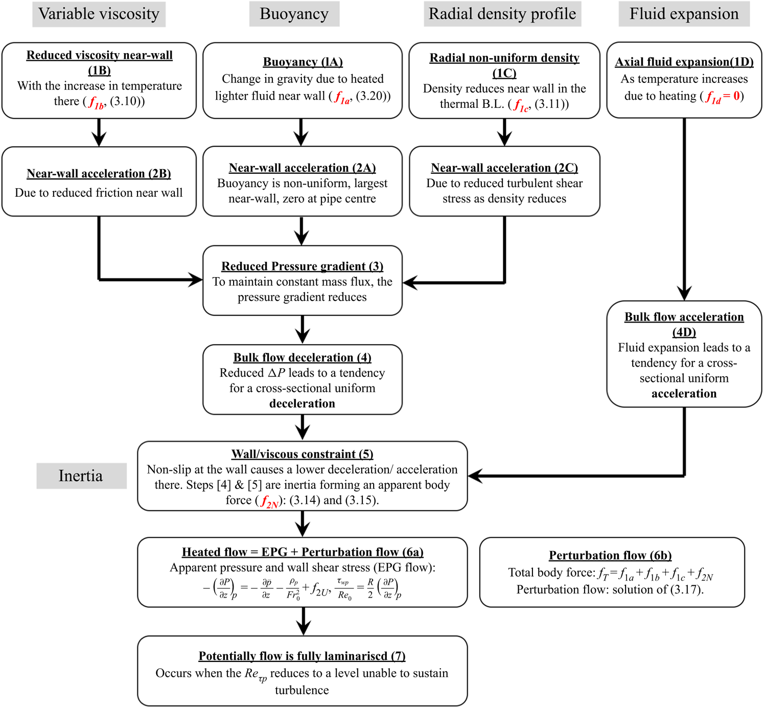
The results presented above suggest that the mechanisms of the flow laminarisation due to buoyancy and variations of density and viscosity can potentially be explained in a unified approach using the ARN theory. It also suggests that the flow inertia plays a significant role, and that it can be viewed as a pseudo-body force, the effect of which can also be explained in the same framework. The overall idea is shown in figure 15, which illustrates how each of the primary mechanisms (buoyancy, variable properties, radial density profile and axial fluid expansion) causes flow changes and how they interact with each other, and especially how they lead to an additional mechanism, inertia, in a spatially developing flow. As in the last two sections, this discussion is for the laminarising stage of the flow and considers only the indirect effect of variable properties on turbulence. The direct effect will be discussed in the next section and it will be seen that the effect in the laminarising stage is relatively small.
A unified explanation for flow laminarisation in a heated flow.

We consider the buoyancy effect first and stages 1A and 2A are well known: the heated fluid near the wall becomes lighter resulting in an upward buoyancy force, which in turn causes the fluid there to accelerate in relation to the fluid in the core. Since we are considering a constant mass flux flow, the local flow acceleration necessitates a reduction in pressure force (gradient) (stage 3) to cause a bulk flow deceleration to compensate it. This deceleration tends to be uniform across all radial locations since the pressure is largely uniform radially away from the immediate inlet (stage 4). The deceleration of the fluid in the region close to the wall is, however, hindered by viscosity and the no-slip condition on the wall. As a result, the deceleration is uniform in the core of the flow but gradually reduces towards the wall, reaching zero on the wall (stage 5). The region of reduced deceleration is initially limited to a small region close to the wall, but it expands away from the wall with distance downstream.
Consequently, there are two non-uniform body forces involved in a heated developing flow (neglecting other effects for now, e.g. considering case CP), the buoyancy body force  $f_{1a}$ and the non-uniform part of inertia,
 $f_{2N}$. With the increase of the combined effect of the buoyancy and inertia, the ARN and the corresponding EPG flow reduce, leading to lower turbulence (stage 6). When the
 $Re_{\tau p}$ continues reducing and reaches a sufficiently low value, turbulence production may be switched off and the flow is then fully laminarised (see further discussion on ‘fully’ in the next section) (stage 7).
Next, considering viscosity, figure 2 shows that it reduces significantly close to the wall along with the increase of the temperature in this region from an early stage following the commencement of heating in case BASE (stage 1B in figure 15). This leads to a reduction in frictional resistance in the wall region, and hence a tendency for the fluid to accelerate there (stage 2B). This is then followed by a process that is very similar to that due to the effect of buoyancy. That is, due to the constant mass flux constraint, the pressure gradient reduces (stage 3), which causes the fluid to decelerate uniformly across the whole cross-section (stage 4); but again the viscosity near the wall restricts the deceleration there (stage 5), and so on. It is clear that both stage 2B and stage 5 cause the velocity profile to be flattened.
Even without considering the structural effects, the (indirect) effects of density variations on the flow dynamics are far reaching, including, buoyancy, flow acceleration caused by fluid expansion and radial non-uniform distribution. These effects can be associated with the buoyancy term, the inertial (spatial acceleration) terms and the turbulent shear stresses of the momentum transport equations (3.13), respectively. The buoyancy has already been extensively discussed. We now turn our attention to the effect of the flow acceleration, a topic that has been investigated by numerous researchers.
It is known that when the hydraulic diameter of the channel is small, the flow acceleration effect is often higher than that of buoyancy under strong heating (e.g. Jiang et al. Reference Jiang, Zhang, Zhao and Shi2008; Jackson Reference Jackson2013; McEligot et al. Reference McEligot, Chu, Bae, Laurien and Yoo2020). The effect comes from the fact that the bulk fluid temperature increases with distance downstream due to heating, which results in a density reduction everywhere across the pipe section (stages 1D/4D). This causes the fluid to accelerate, more strongly near the wall in the entrance region, but mostly uniformly across the radius in downstream locations. The expansion does not directly result in a change in mass flux, and hence, unlike in the cases of the buoyancy and viscosity, there is not a direct consequential reduction in pressure gradient in this case (see figure 15). In fact, to cause the flow acceleration, there is a need for an increase in pressure gradient. Again due to the constraint of the wall/viscosity, the near-wall acceleration is hindered and being smaller than in the centre and hence resulting in a flattened velocity profile (stage 5). It is worth noting that the inertial/viscous effect in this case is opposite to that in the buoyancy and variable viscosity. That is, the viscous effect near the wall hinders the acceleration (rather than deceleration) of the fluid in the pipe and hence the combined effect of stages 4D and 5 causes an apparent body force in the streamwise direction.
Unlike the buoyancy and flow acceleration, the radial non-uniform density distribution associated with the turbulent shear stress terms is seldom explicitly discussed for heated pipe flow at supercritical pressure. This is, however, the effect considered in the van Driest transformation (Van Driest Reference Van Driest1951), and the more recent studies of near wall flow scaling (Patel et al. Reference Patel, Boersma and Pecnik2016; Trettel & Larsson Reference Trettel and Larsson2016). In all these studies, it is assumed that the density variations do not influence turbulence structures under the condition of small fluctuations (the Morkovins hypothesis), which is interpreted as meaning that the mixing length correlation remains unchanged in the scaling analysis. Under this assumption (or, similarly, the eddy viscosity remains largely unchanged), the significant reduction in density near the wall (figure 2) (stage 1C) results in a reduction in flow resistance due to the reduced turbulent shear stress (that is,  $\bar {\rho } \widetilde {u''_{z} u''_{r}}$ reduces because
 $\bar {\rho }$ reduces strongly whereas the changes of the
 $\widetilde {u''_{z} u''_{r}}$ are minor), and hence there is a local flow acceleration in that region (stage 2C). This is then followed by a process that is similar to that in the case of buoyancy and viscosity variations: the local flow acceleration necessitates a reduction in pressure gradient (stage 3) under the constant mass flux constraint, leading to a whole cross-sectional flow deceleration (statge 4), and so on (figure 15).
In summary, the above discussion outlines a unified explanation for the various mechanisms of flow laminarisation in a heated vertical pipe flow. Following a primary cause of change in a heated flow, that is, either the buoyancy, or the variations of density or viscosity, a local change in mass flux occurs near the wall. This then leads to a response in the pressure gradient due to the continuity constraint, which causes a tendency of a uniform bulk fluid acceleration or deceleration balancing the near-wall mass flux changes. The no-slip condition on the wall, however, restrains such changes near the wall, resulting in a smaller acceleration/deceleration there, and hence a distortion in velocity profile. These last stages (stages 4 and 5) are the effects of inertia (spatial acceleration) reflected as the so-called entrance effect, or more generally, a spatially developing flow. The effect of the bulk fluid expansion is slightly simpler, directly causing an inertial effect.
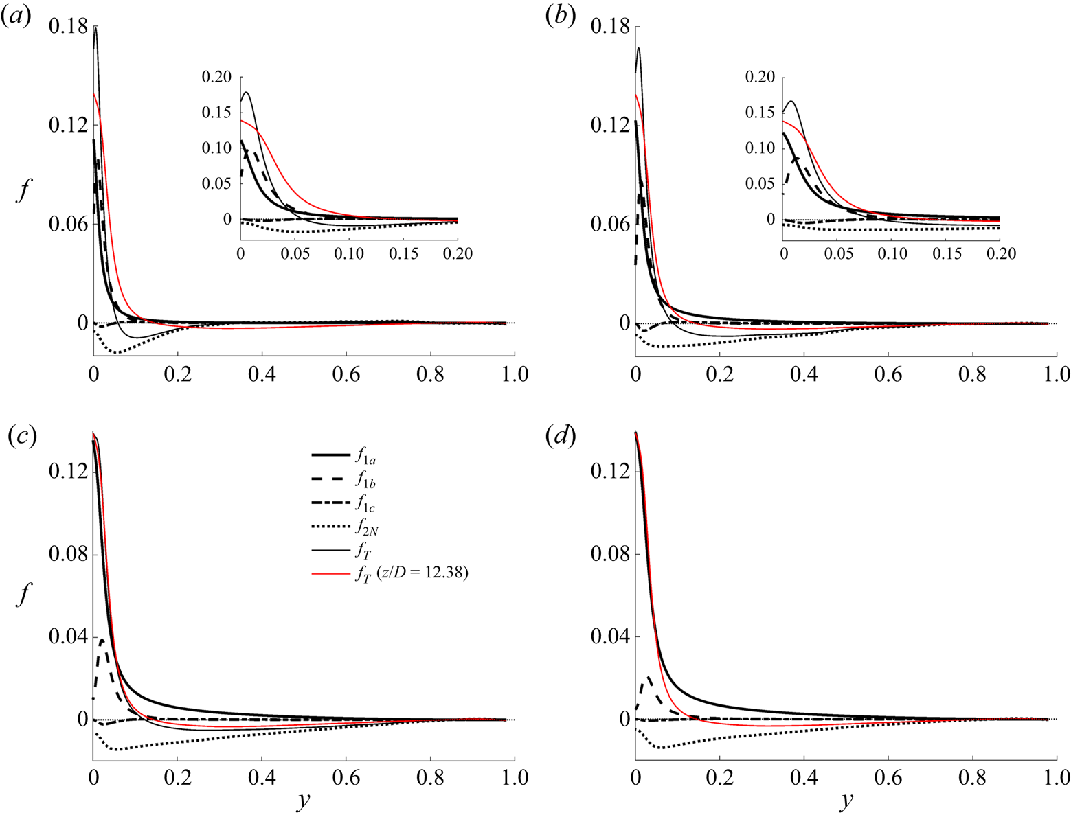
The (pseudo-)body forces at several streamwise locations in case BASE are shown in figure 16. Since (3.17) for the perturbation flow is linear, the different mechanisms act independently and their effects on producing the perturbation flow can simply be added together. It can be seen that in the flow concerned here (case BASE), among the primary causes (first line in figure 15), the buoyancy ( $f_{1a}$) is most significant followed by the variable viscosity (
 $f_{1b}$). The effect of non-uniform density through turbulence shear (
 $f_1c$) is very small. The inertia (
 $f_{2N}$) is always strong and it acts against the primary forces, i.e. reducing or delaying their effects, which is consistent with our understanding. This also explains the differences between the behaviours of the streamwise turbulence stress in the developing flow considered here and those considered in He et al. (Reference He, He and Seddighi2016). The non-uniform body force in the latter causes strong streaks and hence an increase in streamwise turbulence, but the inertia in the flow considered here largely cancel that effect. One can also relate the effects of the positive/negative body forces studied here with the increasing/decreasing
 $Re_\tau ^*$ of Patel et al. (Reference Patel, Boersma and Pecnik2016), although this is outside the scope of this study.
Comparison between the various pseudo-body forces in case BASE at locations (a)  $z/D =2$, (b) 5, (c) 10 and (d) 12.38.

Finally, we note that, even though we have concluded that the non-uniform body force does not directly cause changes in turbulence, it is clear from the above discussion that they are in fact the reasons for flow laminarisation in a fixed mass flux flow, such as the flow considered herein. This is because the total flow comprises the EPG flow plus the non-uniform body-force induced perturbation. As the body forces increase, they cause an increase in the perturbation flow; to maintain the total mass flow rate, the EPG flow reduces, leading to a reduction in turbulence. Hence the greater the non-uniform body forces the stronger the laminarisation.
3.5. ‘Full’ laminarisation and retransition
In this study, the ‘fully’ laminarised region is defined such that the start of the region coincides with the location where the streamwise turbulence reaches its minimum and the end of the region coincides with the location where the transverse (radial and circumferential) Reynolds stresses reach their minima. During this period, the pressure strain is minimum, as shown in figures 5 and 6, where the budgets of the streamwise Reynolds stresses in cases CP and BASE are shown. The full laminarisation occupies  $12< z/D<18$ in case BASE and
 $18< z/D<28$ in case CP. It is clear that in this region turbulence kinetic energy remains very significant in both cases, as mentioned earlier, despite being much lower than that in the unheated flow. The terminology, ‘full’ laminarisation, used here refers to the fact that the turbulence regeneration cycle largely ceases despite there being strong generation of low-speed streaks, as discussed below.
It can be seen from figure 1 that the turbulent shear stress is close to zero everywhere in the cross-section towards the end of this period, i.e. at approximately  $z/D=18$ and
 $28$ in cases CP and BASE, respectively. This is roughly the time when the mean velocity switches from a normal central-peaked profile to an M-shape in which the peak moves away from the pipe centre. The reason that the turbulent shear stress is nearly zero at this stage is that the velocity gradient in most of the flow is very small, except very close to the wall, making the correlation
 $\widetilde {u''_{z} u''_{r} }$ diminish to a minimum. However, the turbulent activities, including mixing for example, are still strong at this stage, and the turbulent heat flux is quite large as well (e.g. see Bae et al. Reference Bae, Yoo and Choi2005).
The shear production remains at a minimum level in the full laminarisation region as can be seen in figures 5 to 7. In case BASE, it approaches zero towards the end of the region, and slowly builds up downstream. Incidentally, there are two peaks now which were also observed in various previous studies (e.g. Bae et al. Reference Bae, Yoo and Choi2005). The near-wall peak is in between the wall and the velocity peak and is the stronger of the two. The second peak in the production is in the core of the flow, where both  $\widetilde {u''_z u''_r}$ and the velocity gradient have changed sign. In case CP, the shear production becomes slightly negative and stays negative for some distance (
 $22< z/D<32$). This is mostly in the near-wall region. Here, the sign of velocity gradient remains unchanged but
 $\widetilde {u''_z u''_r}$ has changed sign. The negative production implies that in this region the shear extracts energy from the turbulent motions and feeds it back to the mean flow, hence leading to an inverse cascade. Towards the end of the simulated domain, the shear production becomes mostly positive across the pipe section with also two peaks as in case BASE.
For both cases CP and BASE, the buoyancy production is small and negative (figures 5 and 6) at the early stages of the heating section (laminarising region). However, it plays a major role in the flow laminarisation and recovery regions, being much stronger than the shear production. Close to the start of the laminarisation stage, the buoyancy production becomes positive, and then increases rapidly with distance, becoming very significant around the point when the shear production is weakest. In case BASE, the peak buoyancy production has maximised at approximately  $z/D=22$, and then reduces gradually with distance downstream. The peak value becomes lower than that of the shear production around
 $z/D=28$. However, the shear production is only significant around the first peak, and is limited to small region (
 $y^{+0}<10$). The buoyancy production, however, peaks at around
 $y^{+0}=12$ and is significant over a bigger region towards the core of the pipe. As a result, in terms of the total cross-sectional contribution, the buoyancy production maintains roughly a constant value from
 $z/D=20$ and is the dominant contributor until the end of the pipe simulated (figure 7). In case CP, the peak of the buoyancy production increases steadily throughout the later part of the pipe. The cross-sectional integration increases significantly downstream due to the spread of the region where the production is significant. Consequently these results demonstrate that the buoyancy production is responsible for the regeneration of turbulence and the dominant contributor to the continuing increase of turbulence further downstream.
We now look at the flow from the viewpoint of transition. Similar to the shear production, the production due to buoyancy is only significant in the streamwise Reynolds stress ( $\overline {u'^{2}_z}$) and the energy produced is then re-distributed through pressure-strain work to other components. In case BASE, the buoyancy production becomes positive at approximately
 $z/D=12$ (figure 7), which is roughly coincident with the location where
 $\overline {u'^{2}_z}$ is the lowest (figure 12). The energy in
 $\overline {u'^{2}_z}$ starts to increase near the wall after this point clearly due to the buoyancy production. The transverse Reynolds stresses (
 $\overline {u'^2_r}$ and
 $\overline {u'^{2}_\theta }$), however, continue to reduce until around
 $z/D=18$. This observation is consistent with that in the bypass transition in transient flow (He & Seddighi Reference He and Seddighi2013, Reference He and Seddighi2015). The initial generation of
 $\overline {u'^{2}_z}$ (
 $z/D=12$ to
 $18$) is likely linked to the formation and elongation of high- and low-speed streaks. Only at around
 $z/D=18$, such streaks start breaking down, forming turbulent spots where vortices of various small scales are generated. This process can be viewed in figure 3, where turbulence structures are visualised using isosurface/cross-sectional plots of
 $u'_z$,
 $\lambda _2$ and density. In case BASE, between
 $z/D=12$ and 18, even though the
 $u'_{z}$ increases significantly the turbulence vortices remain the lowest, and they start to reappear in significant quantities only after
 $z/D=18$. In case CP, the turbulent vortices remain very low over a large section of the pipe and the regeneration of turbulence remains weak even at the end of the simulated domain. Additionally, figure 17 shows a quadrants analysis for the turbulent activities in case BASE, in which both weak (
 $H=0$) and strong events (high
 $H=2$, 4) are shown for the ejection (
 $Q_2$) and sweep events (
 $Q_4$). Both events reach very low level (especially the strong events) during the full laminarisation stage. However, sweeps appear to reach its minimum at the middle of this region and start to increase gradually at the second half-region, while the ejections only start to recover some distance after the end of this region. For case CP, the buoyancy production becomes positive at around
 $z/D=19$, which again coincides with the location where
 $\overline {u'^2_z}$ is the lowest. The value of
 $\overline {u'^2_z}$ starts to increase rapidly following this but the transverse components continue to reduce until about
 $z/D=30$. During all of this stage (
 $z/D>19$), the shear production is either very low or slightly negative, and turbulence is mostly generated due to buoyancy production.
Quadrant analysis for the plane  $y^{+0}=15.2$ in case BASE (a) quadrant 2 (
 $Q_2$) and (b) quadrant 4 (
 $Q_4$).

It can now be concluded that in the ‘fully’ laminarised flow region, the coupled sequential streak and vortex generation of the turbulence regeneration cycle associated with the initial shear flow has largely ceased. The pressure strain also approaches zero, indicating that the vorticity generation has become minimum. Nevertheless, turbulence fluctuations are still in existence. In fact, right from the start of this stage, buoyancy turbulence generation has started in the form of new elongated streaks, which leads to an increase in  $\overline {u'^{2}_z}$ in the wall region. Consequently, the region of laminarisation discussed here is not completely consistent with that used commonly in the literature in which laminarisation normally refers to zero turbulence kinetic energy or turbulence production. The re-transition considered herein refers to the stage where new turbulence spots and multi-scale vortical structures start appearing, which may be significantly later than the initial recovery of turbulence kinetic energy related to the generation of streaks, an phenomenon occurs at the pre-transition stage.
During the full laminarisation stage, the energy of streamwise turbulence at locations away from the wall, and the transverse turbulence components everywhere, continue decaying. In fact, in the core region, the turbulence behaves in a manner similar to the decay of grid generated homogeneous turbulence, which is known to behave as  $k/U^2=c((x-x_0)/M)^{-n}$, where k is turbulence kinetic energy,
 $U$ is the uniform-stream velocity,
 $M$ the mesh spacing,
 $x_0$ the virtual origin and
 $n$ is between 1.15 and 1.45 (Pope Reference Pope2001). The transport equations for turbulence kinetic energy and its dissipation for such a flow can be written as
 \begin{equation} U \frac{\partial k}{\partial z}={-}\epsilon,\quad U \frac{\partial \epsilon}{\partial z}={-}C_{\epsilon 2} \frac{\epsilon^2}{k}, \end{equation}
where  $C_{e2} = 1.9$. The above also suggests that
 $\epsilon \propto x^{-(n+1)}$. It can be seen from figure 18 that turbulence kinetic energy in the core of the pipe (
 $r<0.4$) during the ‘full’ laminarised region indeed decays in an exponential manner. But the exponent is significantly highly than that of a grid turbulence, being around 2. Consistently, the turbulence dissipation decays also exponentially with an exponent of 3. Additionally, we have computed
 $C_{e2}$ from (3.21a,b), (that is assuming a convective decaying turbulence). The value is mostly between
 $1.5$ and
 $2.0$ in the fully laminarised region but is significantly different from this value elsewhere. The observation described above is typical of the pre-transition stage of boundary layer bypass transition in which elongated streaks are formed within the boundary layer whereas the free-stream turbulence decays exponentially (Andersson et al. Reference Andersson, Brandt, Bottaro and Henningson2001; Jacobs & Durbin Reference Jacobs and Durbin2001; Fransson, Matsubara & Alfredsson Reference Fransson, Matsubara and Alfredsson2005).
Decay of the turbulence kinetic energy and its dissipation rate in cases CP (a,c) and BASE (b,d).

4. Summary and conclusions
DNS of a heated flow of  $\text {CO}_2$ in a pipe at a supercritical pressure has been analysed in this paper. New understanding has been established of the turbulence dynamics with respect to its three-stage development, that is, partially laminarising, full laminarisation and re-transition stages. The main findings are as follows:
• The effects of buoyancy and variations of density and viscosity on turbulence (and laminarisation) together with the effects of inertia are explained using a unified approach based on the apparent Reynolds number (ARN) and non-uniform (pseudo-) body-force concepts first introduced by He et al. (Reference He, He and Seddighi2016) for an isothermal flow. The partially laminarising flow is represented by an equivalent pressure gradient (EPG) base flow plus a perturbation caused by the various mechanisms, all of which are represented using (pseudo-)body forces.
• In the ‘full’ laminarisation region referred to in this paper the turbulence regeneration cycle has ceased, but typically turbulence kinetic energy is still significant in the flow. There can still be strong turbulence generation due to buoyancy production, resulting in the generation of high-/low-speed streaks near the wall and hence some increase in the streamwise fluctuating velocity, but not in the transverse components. Away from the wall, turbulence decays exponentially with downstream distance.
• Transition is marked by the generation of the transverse (radial and circumferential) turbulence components and the associated increase of pressure strain in the Reynolds stress budgets.
The above is further expanded below with the key points illustrated in figure 19.
An overview of turbulence dynamics in a heated flow with laminarisation.

4.1. Partial flow laminarisation
The partial flow laminarising region occupies  $z/D<12$ in case BASE and
 $z/D<18$ in case CP. The flow at any streamwise location can be represented by its equivalent pressure gradient (EPG) flow and a perturbation flow caused by the pseudo-body forces due to the various mechanisms. The stronger the buoyancy or property variations, the greater the pseudo-body forces, which in turn causes a larger perturbation flow. For the flow in a pipe with a fixed mass flux, this means a smaller EPG flow, and hence lower turbulence. When the Reynolds number of the EPG flow (i.e. the
 $Re_{\tau p}$) reduces to a very low level (say,
 $<$80), the flow may be fully laminarised. In this theory, the laminarising flow can be estimated using the knowledge of the EPG flow and the (pseudo-)body forces without solving the non-equilibrium turbulent flow. This theory is based on the hypothesis that the buoyancy, variable properties and the inertia do not alter the key turbulence characteristics, including the mixing effect, in comparison with that in the EPG flow. It then follows straightforwardly that all effects can be expressed as a pseudo-body force. The hypothesis was shown in He et al. (Reference He, He and Seddighi2016) to be true for non-uniform body forces in an isothermal flow. With regard to the effect of variations of density and viscosity, a similar hypothesis was proposed and used in previous studies, including Huang et al. (Reference Huang, Coleman and Bradshaw1995), Trettel & Larsson (Reference Trettel and Larsson2016), Patel et al. (Reference Patel, Boersma and Pecnik2016) and the well-known van Driest transformation (for density only) (Coleman et al. Reference Coleman, Kim and Moser1995). In the present study, the hypothesis has been extended to include not only all the physical effects (variable properties and buoyancy), but also the spatial acceleration, hence establishing a unified explanation for the laminarisation in a heated flow. The hypothesis is demonstrated in § 3.2 to be true using the Boussinesq assumption based flow (case CP) and a flow with a full account of all thermophysical property variations (case BASE).
There are a number of primary causes (mechanisms) that make heated vertical flow different from an unheated flow, that is, the buoyancy, the variations of viscosity, the flow acceleration due to fluid expansion caused by heating and the radial variation of density resulting in a change in turbulent shear (figure 15). The way they influence the flow can be seen through the momentum equations: that is, the gravitational force, the viscous diffusion terms, the spatial acceleration (convection) terms and the turbulent shear stresses. Each effect can be represented by a (pseudo-)body force. They all influence the flow in a similar manner but independently of each other and their effects can be linearly added up. Together, they cause an overall perturbation flow which can be computed knowing the body forces and the EPG flow. The fluid expansion-caused acceleration directly results in a change in the inertia, which is discussed below.
The spatial acceleration (inertia) is strong in such a developing flow and its effect on turbulence can again be treated as a pseudo-body force. It has two components. The uniform component is a direct response to a change in pressure gradient (effectively ‘cancelling’ it partially) and this term can be grouped with the pressure and the uniform gravitational component, forming a total modified pressure gradient. The non-uniform component acts like other (pseudo-)body forces, having no direct influence on the turbulence but a mean perturbation flow. The inertia is a response of the flow to the primary causes as shown in figure 15. The direction of the inertia is opposite to the other effects, and delays or partially cancels the reduction of turbulence due to other effects.
When normalised using the apparent friction velocity, the eddy viscosity and the transverse turbulence components remain largely the same at any location in the laminarising region. Hence, the primary turbulence dynamics and mixing under this normalisation are not significantly modified by the effects of buoyancy, property variations and flow development; and they can be reasonably well represented by those of the EPG reference flow. The turbulent shear stress can be reasonably well evaluated using the EPG flow statistics. The streamwise turbulent stress normalised in the same way, however, does change with streamwise distance. This is a reflection of the additional production of the high-/low-speed streaks due to the perturbation flow caused by the pseudo-body forces.
The flow is ‘non-equilibrium’, that is, it is developing with distance and the inertia is a significant contributor to the momentum balance. The turbulence, however, is approximately in equilibrium and the convection is insignificant, although the turbulence anisotropy may be different from that in an unheated flow due to the generation of streaks.
In this region, buoyancy production (i.e. the structural effect) causes some turbulence reduction even though it is relatively small in comparison with other budget terms. Incidentally, the contribution of the buoyancy production and the convection to turbulence budget are opposite and partly cancel each other, making the net effect smaller. This, to some extent, contributes to the success of the unified explanation, which implicitly assumes that turbulence is in equilibrium in the sense that it is not affected by up-/downstream turbulence and the structural effect is insignificant.
4.2. Full laminarisation
This region can be compared with the pre-transition region of boundary layer bypass transition: the free-stream/core turbulence decays, but high-/low-speed streaks are formed near the wall with little vorticity generation. This region extends across the range  $12< z/D<18$ for case BASE and
 $18< z/D<29$ for case CP.
Turbulence kinetic energy in the pipe core ( $r<0.4$) reduces exponentially following
 $k/u^2_z=c((x-x_0)/M)^{-n}$, similar to that of a grid turbulence but with a greater exponent of
 $n=2$ (cf. 1.15 to 1.45 for grid turbulence). Correspondingly, the dissipation also reduces exponentially with an exponent of 3.
The streaks are generated mostly due to buoyancy production but with small shear production at the later stage of this phase. The streaks lead to an increase in the streamwise turbulent stress in the wall regain but not in the transverse turbulent stresses. The ejections/sweeps and the pressure-strain term reduce to and stay at a minimum. The shear production reaches minimum or even negative values. The transverse turbulent stresses reach minimum.
Here, ‘full laminarisation’ refers to the fact that there are no new vortical structures (turbulent spots) produced, but the actual turbulence (turbulence kinetic energy and turbulent mixing) can still be strong due to the decaying turbulence and new streaks. In relation to the latter, the total (shear + buoyancy) production of turbulence may be very strong, resulting in streaks but not multi-scale vortices. Consequently, the use of the term ‘full laminarisation’ here emphasises the stoppage of the turbulence regeneration cycle. This use is different from other common uses, which often refer to no turbulence generation or presence of turbulence kinetic energy.
4.3. Re-transition
Similar to boundary layer bypass transition, new multi-scale vortical structures are generated in this region due to flow instability potentially linked to streaks, although this is not studied in this paper. This region extends across the range  $z/D>18$ for case BASE and
 $z/D>29$ for case CP.
The transition is clearly visualised using instantaneous flow data, which show the breakup of streaks and generation of turbulence spots. With respect to the statistics, this process is reflected as an increase in the pressure-strain action and transverse turbulence components. Buoyancy generation is still dominating in this region but shear production has increased significantly. In fact, the local peak shear production is more than double that of the buoyancy production towards the end in case BASE, although the shear production is still small in case CP. There are two peaks in the shear production in both cases CP and BASE, but the near-wall peak is far greater than that in the outer region.
4.4. The applicability of the findings of this research
The main findings of the present research centre on the unified explanation for the various flow laminarisation mechanisms in a heated developing flow. This can be viewed as an extension of a number of previous studies. The principal assumption is related to the ARN and the use of non-uniform body forces to explain all of these effects. Importantly, it is assumed that the addition of a non-uniform (pseudo-)body force does not cause significant changes in the key turbulence characteristics. This was initially established in He et al. (Reference He, He and Seddighi2016) based on prescribed linear and step profiles of body forces in an isothermal flow. This theory was found to predict well the laminarisation of the heated flows simulated using DNS in Marensi et al. (Reference Marensi, He and Willis2021), in which it was found to be also consistent with the linear instability analysis. Marensi et al.'s study was based on the Boussinesq assumption and hence only the buoyancy effect was considered. On the other hand, the effect of variable density has been studied extensively (Van Driest Reference Van Driest1951; Coleman et al. Reference Coleman, Kim and Moser1995; Huang et al. Reference Huang, Coleman and Bradshaw1995) and to a lesser extent the effect of variable viscosity as well (Trettel & Larsson Reference Trettel and Larsson2016; Patel et al. Reference Patel, Boersma and Pecnik2017) under conditions when buoyancy is not significant or is omitted. A common goal of these studies is to find a suitable normalisation so that the non-dimensionalised turbulence is unchanged from that of the equivalent constant-property flow.
All the above effects co-exist in the flow considered herein, which is further complicated by the streamwise flow development. The test case selected undergoes full laminarisation and heat transfer deterioration followed by recovery due to strong variations of fluid properties under a supercritical pressure condition. In studying such a severe condition, it is expected that the analysis developed in this work can be widely applied to heated pipe flow in general. However, the unified explanation and the ARN concept are not exact solutions but approaches and explanations illustrating the primary effects. Even though they successfully illustrate the key mechanisms with good quantitative agreements (e.g. figures 12 and 13), there are clear discrepancies between the ‘predictions’ and the DNS results as seen in the same figures. A contributor to this is likely to be the fact that the turbulence is not in complete ‘equilibrium’ and the streamwise convection has some effect, as discussed earlier. Consequently, it would certainly be useful in future to study a variety of flow conditions, including for example higher Reynolds numbers. It is perhaps also useful to note that the variation of the applicability of the findings of this study would mean that the discrepancies between the ‘predictions’ and the physical flows would vary and may become greater under certainly conditions, but even under such conditions the analysis approaches would not ‘fail’. It would simply mean that additional factors could be taken into consideration to improve the analysis.
Acknowledgements
J.H. gratefully acknowledges the PhD studentship provided by EDF Energy. The authors gratefully acknowledge the help provided by Dr W. Wang on CHAPSim and the fruitful discussions with Professor W. Ambrosini on the topic of this paper over several years and his comments on the draft manuscript.
Funding
This work used the ARCHER UK National Supercomputing Service (http://www.archer.ac.uk), provided via the UK Turbulence Consortium (grant EP/R029326/1). New developments on CHAPSim have been carried out under the Collaborative Computational Project for Nuclear Thermal Hydraulics (CCP NTH) (EP/T026685/1).
Declaration of interests
The authors report no conflict of interest.
Author contributions
JH: Coding and simulations, data analysis and investigations; writing: review and editing. RT: partial data analysis; writing: review and editing. PXJ: conceptualisation; writing: review and editing. SH: conceptualisation; data analysis and investigations; writing: original draft.
Appendix A. The suitability of the mesh resolution
The suitability of the mesh resolution of the present simulations is discussed here by comparing our simulations with those of Bae et al. (Reference Bae, Yoo and Choi2005) and Nemati et al. (Reference Nemati, Patel, Boersma and Pecnik2015). The inlet Reynolds number of the present cases is 2617 which is slightly lower than that of the cases of Bae et al., at 2700. Here, we have simulated cases B and D of Bae et al. using the mesh used for cases CP and BASE presented in this paper. The mesh resolution used in the present study is similar to that of Bae et al. (Reference Bae, Yoo and Choi2005) and both are coarser than that of Nemati et al. (see table 1).
Mesh resolution. All values are based on inlet flow conditions.

The comparison of the predictions of the wall temperature is shown in figure 20. It can be seen that the results of the Nemati et al. and our own results agree very well for both cases, whereas both are somewhat lower than those of Bae's for case B. Figure 21 shows a further comparison between the turbulent shear stresses predicted by Nemati and those using our mesh at a number of streamwise locations. The agreement is again good in both cases.
Wall temperature in the Bae et al. (Reference Bae, Yoo and Choi2005) cases B and D – comparison between predictions of Bae et al. (Reference Bae, Yoo and Choi2005), Nemati et al. (Reference Nemati, Patel, Boersma and Pecnik2015) and CHAPSim.

Turbulent shear stresses in the Bae et al. (Reference Bae, Yoo and Choi2005) (a) case B and (b) case D – comparison between predictions of Nemati et al. (Reference Nemati, Patel, Boersma and Pecnik2015) and those of CHAPSim.

Appendix B. The transport equation of the streamwise turbulent stress
The transport equation for the normal stress  $\widetilde {u''_z u''_z}$ in cylindrical coordinates can be written as follows:
 \begin{equation} \frac{\partial \bar{\rho} \widetilde{u''_z u''_z} }{\partial t} + C = P + TD + \varPi + \varPhi + VD - \epsilon + G + E, \end{equation}
where
 \begin{equation} \left.\begin{gathered}
C= \frac{\partial \overline{ \rho u''_{z} u''_{z} }
\tilde{u}_{z}}{\partial z} + \frac{1}{r} \frac{\partial r
\overline{\rho u''_{z} u''_{z}} \tilde{u}_{r}}{\partial
r} + \frac{1}{r} \frac{\partial \overline{ \rho u''_{z}
u''_{z} } \tilde{u}_{{\theta}}}{\partial {\theta}},\\
P={-}2 \overline{\rho u''_{z} u''_{z}} \frac{\partial
\tilde{u}_{z}}{\partial z} -2 \overline{\rho u''_{z}
u''_{r}} \frac{\partial \tilde{u}_{z}}{\partial r}
-\frac{2}{r} \overline{\rho u''_{z} u''_{\theta}}
\frac{\partial \tilde{u}_{z}}{\partial {\theta} },\\
TD={-} \frac{\partial \overline{ \rho u''_{z} u''_{z}
u''_{z}} }{\partial z} - \frac{1}{r} \frac{\partial r
\overline{\rho u''_{z} u''_{z} u''_{r}}}{\partial r} -
\frac{1}{r} \frac{\partial \overline{ \rho u''_{z} u''_{z}
u''_{\theta} } }{\partial {\theta}},\\ \varPi ={-}2
\frac{\partial \overline{ p' u''_{z}} }{\partial z}, \quad
\varPhi= 2 \overline{ p' \frac{\partial u''_{z}}{\partial
z} },\\ VD = 2 \frac{\partial \overline{u''_z
\tau'_{zz}}}{\partial z} + \frac{2}{r} \frac{\partial r
\overline{u''_z \tau'_{zr}}}{\partial r} + \frac{2}{r}
\frac{\partial \overline{u''_z \tau'_{r \theta}}}{\partial
\theta},\\ \epsilon= 2 \overline{\tau'_{zz} \frac{\partial
u''_z}{\partial z}} + 2\overline{\tau'_{zr} \frac{\partial
u''_z}{\partial r} } + \frac{2}{r}
\overline{\tau'_{z\theta} \frac{\partial u''_z}{\partial
\theta} },\\ G ={-}2 \frac{\partial \overline{p}}{\partial
z} \overline{u''_{z}}, \quad E = 2 \overline{u''_z}
\frac{\partial \overline{\tau_{zz}}}{\partial z} +
\frac{2}{r} \overline{u''_z} \frac{\partial r
\overline{\tau_{zr}}}{\partial r} + \frac{2}{r}
\overline{u''_z} \frac{\partial
\overline{\tau_{z\theta}}}{\partial \theta}.
\end{gathered}\right\}
\end{equation}
Equation (B1) includes the convection  $C$, turbulence production
 $P$, turbulence diffusion
 $TD$, pressure diffusion
 $\varPi$, pressure strain
 $\varPhi$, viscous diffusion
 $VD$, dissipation
 $\epsilon$, pressure work (this is mostly buoyancy production and referred to as such in the paper)
 $G$ and an additional term due to velocity fluctuations
 $E$.