2.1 Lorentz transformation to the pulsar frame

The Lorentz transformation from the unprimed frame ${\mathcal{K}}$ to the primed frame ${\mathcal{K}}^{\prime }$ moving along the magnetic field at speed $\unicode[STIX]{x1D6FD}_{\text{s}}$ applied to a wave, described by frequency $\unicode[STIX]{x1D714}$ and components $k_{\Vert }$ and $k_{\bot }$ , parallel and perpendicular, respectively, to the relative velocity, gives

(2.1a-c ) $$\begin{eqnarray}\unicode[STIX]{x1D714}^{\prime }=\unicode[STIX]{x1D6FE}_{\text{s}}(\unicode[STIX]{x1D714}+k_{\Vert }c\unicode[STIX]{x1D6FD}_{\text{s}}),\quad k_{\Vert }^{\prime }c=\unicode[STIX]{x1D6FE}_{\text{s}}(k_{\Vert }c+\unicode[STIX]{x1D714}\unicode[STIX]{x1D6FD}_{\text{s}}),\quad k_{\bot }^{\prime }=k_{\bot },\end{eqnarray}$$

with $\unicode[STIX]{x1D6FE}_{\text{s}}=(1-\unicode[STIX]{x1D6FD}_{\text{s}}^{2})^{-1/2}$ . In terms of the variables $z=\unicode[STIX]{x1D714}/k_{\Vert }c$ and $\unicode[STIX]{x1D703}$ in the unprimed frame, ${\mathcal{K}}$ , and $z^{\prime }=\unicode[STIX]{x1D714}^{\prime }/k_{\Vert }^{\prime }c$ and $\unicode[STIX]{x1D703}^{\prime }$ in the primed frames, ${\mathcal{K}}^{\prime }$ , equations (2.1) and the inverse transforms imply

(2.2a-d ) $$\begin{eqnarray}z^{\prime }=\frac{z+\unicode[STIX]{x1D6FD}_{\text{s}}}{1+\unicode[STIX]{x1D6FD}_{\text{s}}z},\quad z=\frac{z^{\prime }-\unicode[STIX]{x1D6FD}_{\text{s}}}{1-\unicode[STIX]{x1D6FD}_{\text{s}}z^{\prime }},\quad \tan \unicode[STIX]{x1D703}^{\prime }=\frac{\tan \unicode[STIX]{x1D703}}{\unicode[STIX]{x1D6FE}_{\text{s}}(1+\unicode[STIX]{x1D6FD}_{\text{s}}z)},\quad \tan \unicode[STIX]{x1D703}=\frac{\tan \unicode[STIX]{x1D703}^{\prime }}{\unicode[STIX]{x1D6FE}_{\text{s}}(1-\unicode[STIX]{x1D6FD}_{\text{s}}z^{\prime })}.\end{eqnarray}$$

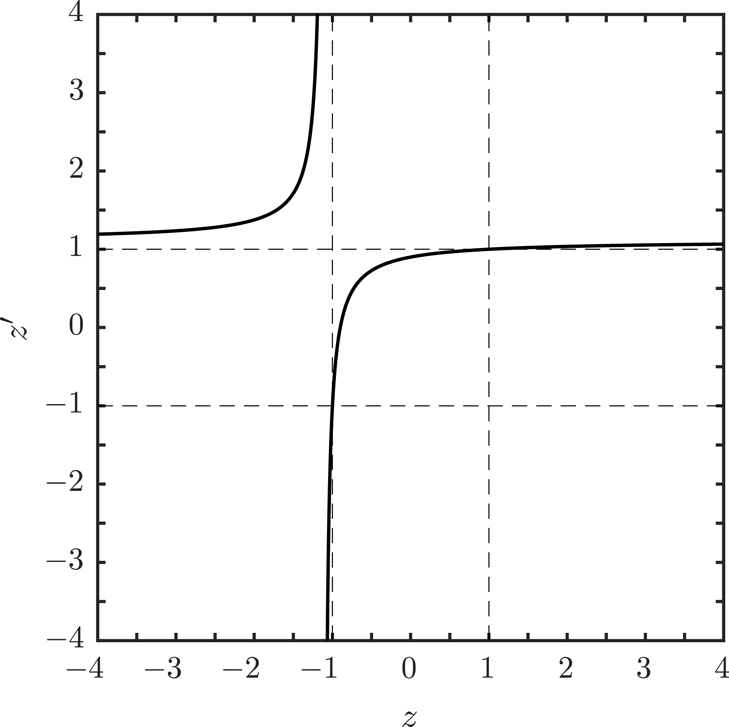
The relation between $z^{\prime }$ and $z$ is illustrated (for $\unicode[STIX]{x1D6FD}_{\text{s}}=0.9$ ) in figure 1. The relation separates into two branches. One branch includes the subluminal range, $-1<z<1$ with $-1<z^{\prime }<1$ , and two superluminal ranges, one where both $z,z^{\prime }$ are negative, $-1/\unicode[STIX]{x1D6FD}_{\text{s}}<z<-1$ with $-\infty <z^{\prime }<-1$ , and another where both $z,z^{\prime }$ are positive, $1<z<\infty$ with $1<z^{\prime }<1/\unicode[STIX]{x1D6FD}_{\text{s}}$ . The other branch is for superluminal negative $z$ and superluminal positive $z^{\prime }$ , $-\infty <z<-1/\unicode[STIX]{x1D6FD}_{\text{s}}$ with $1/\unicode[STIX]{x1D6FD}_{\text{s}}<z^{\prime }<\infty$ , respectively. Assuming a source on the near side of the pulsar, only waves with $z^{\prime }>0$ can reach the observer; these include not only forward-propagating waves, $z>0$ , in ${\mathcal{K}}$ but also backward-propagating waves with $-\unicode[STIX]{x1D6FD}_{\text{s}}<z<0$ in ${\mathcal{K}}$ , which become forward-propagating waves, $z^{\prime }>0$ , in ${\mathcal{K}}^{\prime }$ .

Figure 1.

The relation (2.2) between $z^{\prime }$ and $z$ is plotted for $\unicode[STIX]{x1D6FD}_{\text{s}}=0.9$ ; the box enclosed by the dashed lines at $z,z^{\prime }=\pm 1$ is the subluminal range.

2.2 Subluminal waves

The subluminal range $-1<z<+1$ in ${\mathcal{K}}$ maps onto the subluminal range $-1<z^{\prime }<+1$ in ${\mathcal{K}}^{\prime }$ . However, $z^{\prime }$ and $z$ can have opposite signs. The phase speed $z=0$ ( $z^{\prime }=0$ ) that separates forward- and backward-propagating waves in ${\mathcal{K}}$ (in ${\mathcal{K}}^{\prime }$ ) maps onto $z^{\prime }=\unicode[STIX]{x1D6FD}_{\text{s}}$ ( $z=-\unicode[STIX]{x1D6FD}_{\text{s}}$ ) in ${\mathcal{K}}^{\prime }$ (in ${\mathcal{K}}$ ). Forward-propagating waves with $0<z^{\prime }<\unicode[STIX]{x1D6FD}_{\text{s}}$ in ${\mathcal{K}}^{\prime }$ correspond to backward-propagating waves $-\unicode[STIX]{x1D6FD}_{\text{s}}<z<0$ in ${\mathcal{K}}$ . However, this interpretation requires further comment. Note that the inverse of the transformation given by (2.1), specifically $\unicode[STIX]{x1D714}=\unicode[STIX]{x1D6FE}_{\text{s}}\unicode[STIX]{x1D714}^{\prime }(z^{\prime }-\unicode[STIX]{x1D6FD}_{\text{s}})/z^{\prime }$ and $k_{\Vert }c=\unicode[STIX]{x1D6FE}_{\text{s}}k_{\Vert }^{\prime }c(1-z^{\prime }\unicode[STIX]{x1D6FD}_{\text{s}})$ , implies that $z$ has the opposite sign to $z^{\prime }$ due to $\unicode[STIX]{x1D714}<0$ , $k_{\Vert }>0$ . The negative frequency requires interpretation.

It is conventional to describe a wave in terms of a positive frequency, and it is always possible to do so because the dispersion equation is unchanged under $\unicode[STIX]{x1D714},k_{\Vert }\rightarrow -\unicode[STIX]{x1D714},-k_{\Vert }$ and hence is an even function of $z$ with positive- and negative-frequency solutions $\unicode[STIX]{x1D714}=\pm \unicode[STIX]{x1D714}_{M}(z)$ , for some wave mode $M$ . Confusion arises because negative $z$ can be due to either $\unicode[STIX]{x1D714}$ or $k_{\Vert }$ being negative. A formal way of allowing for the change in sign of the frequency under a Lorentz transformation is to distinguish between forward- and backward-propagating wave modes with dispersion relations $\unicode[STIX]{x1D714}=\unicode[STIX]{x1D714}_{M\pm }(z)>0$ . One then requires that if the Lorentz transformation causes the frequency to change sign, one reinterprets this as a change in mode, from forward propagating, $M+$ , to backward propagating, $M-$ .

The mapping $z\rightarrow z^{\prime }$ for $\{1-|z|,1-|z^{\prime }|\}\ll 1$ becomes strongly distorted for $\unicode[STIX]{x1D6FE}_{\text{s}}\gg 1$ . Important features of the wave dispersion discussed in Part 1 occur for $\unicode[STIX]{x1D6FE}_{\unicode[STIX]{x1D719}}=(1-z^{2})^{-1/2}\gg 1$ , and an approximate form for the Lorentz transformation is desirable for this case. The relations (2.2) for $\{1-|z|,\unicode[STIX]{x1D703}\}\ll 1$ may be approximated by

(2.3a-c ) $$\begin{eqnarray}\unicode[STIX]{x1D714}^{\prime }\approx 2\unicode[STIX]{x1D6FE}_{\text{s}}\unicode[STIX]{x1D714},\quad \unicode[STIX]{x1D6FE}_{\unicode[STIX]{x1D719}}^{\prime }\approx 2\unicode[STIX]{x1D6FE}_{\unicode[STIX]{x1D719}}\unicode[STIX]{x1D6FE}_{\text{s}},\quad \unicode[STIX]{x1D703}^{\prime }\approx \unicode[STIX]{x1D703}/2\unicode[STIX]{x1D6FE}_{\text{s}},\end{eqnarray}$$

where we assume $\{\unicode[STIX]{x1D6FE}_{\unicode[STIX]{x1D719}},\unicode[STIX]{x1D6FE}_{\text{s}}\}\gg 1$ . Thus phase speeds $z\approx 1$ near the speed of light, $\unicode[STIX]{x1D6FE}_{\unicode[STIX]{x1D719}}\gg 1$ , in ${\mathcal{K}}$ transform into phase speeds much closer to the speed of light, $\unicode[STIX]{x1D6FE}_{\unicode[STIX]{x1D719}}^{\prime }\approx 2\unicode[STIX]{x1D6FE}_{\text{s}}\unicode[STIX]{x1D6FE}_{\unicode[STIX]{x1D719}}\gg \unicode[STIX]{x1D6FE}_{\unicode[STIX]{x1D719}}$ , in ${\mathcal{K}}^{\prime }$ .

The approximation (2.3) applies to the forward-propagating, $z>0$ , parallel Alfvén (or A) mode, with the dispersion relation $z=z_{\text{A}}\approx 1+1/2\unicode[STIX]{x1D6FD}_{\text{A}}^{2}$ transforming into $z^{\prime }=z_{\text{A}}^{\prime }$ , $z_{\text{A}}^{\prime }=(z_{\text{A}}+\unicode[STIX]{x1D6FD}_{\text{s}})/(1+z_{\text{A}}\unicode[STIX]{x1D6FD}_{\text{s}})\approx 1+1/2\unicode[STIX]{x1D6FD}_{\text{A}}^{\prime 2}$ , with $\unicode[STIX]{x1D6FD}_{\text{A}}^{\prime }\approx 2\unicode[STIX]{x1D6FE}_{\text{s}}\unicode[STIX]{x1D6FD}_{\text{A}}$ . Similarly, the maximum frequency of the L mode is determined by the maximum of the RPDF, at $z=z_{\text{m}}$ with $\unicode[STIX]{x1D6FE}_{\unicode[STIX]{x1D719}}=\unicode[STIX]{x1D6FE}_{\text{m}}$ in ${\mathcal{K}}$ , and at $z^{\prime }=z_{\text{m}}^{\prime }=(z_{\text{m}}+\unicode[STIX]{x1D6FD}_{\text{s}})/(1+z_{\text{m}}\unicode[STIX]{x1D6FD}_{\text{s}})$ , with $\unicode[STIX]{x1D6FE}_{\unicode[STIX]{x1D719}}^{\prime }=\unicode[STIX]{x1D6FE}_{\text{m}}^{\prime }\approx 2\unicode[STIX]{x1D6FE}_{\text{s}}\unicode[STIX]{x1D6FE}_{\text{m}}$ in ${\mathcal{K}}^{\prime }$ . The features of the wave dispersion in the small range of $0<1-z\ll 1$ , with $z>0$ , discussed in Part 1 are squeezed into an extremely narrow range (smaller by a factor $1/2\unicode[STIX]{x1D6FE}_{\text{s}}$ ) of phase speeds $0<1-z^{\prime }\ll 1$ in ${\mathcal{K}}^{\prime }$ .

2.3 Superluminal waves

The superluminal ranges in ${\mathcal{K}}$ and ${\mathcal{K}}^{\prime }$ also map into each other, but in a less obvious way than for subluminal waves. In this case changes in sign between $z$ and $z^{\prime }$ occur at $(z,z^{\prime })=(\pm \infty ,1/\unicode[STIX]{x1D6FD}_{\text{s}})$ , or at $(z,z^{\prime })=(-1/\unicode[STIX]{x1D6FD}_{\text{s}},\pm \infty )$ . The frequency cannot change sign, and the introduction of $\pm$ modes is not relevant. In this case, $k_{\Vert }^{\prime }$ changes sign, relative to $k_{\Vert }$ , at $z=-1/\unicode[STIX]{x1D6FD}_{\text{s}}$ causing backward-propagating waves in ${\mathcal{K}}$ with $z<-1/\unicode[STIX]{x1D6FD}_{\text{s}}$ to become forward propagating in ${\mathcal{K}}^{\prime }$ .

In the application to pulsars, superluminal waves are relevant to oscillations that are primarily in time. Purely temporal oscillation correspond to $k_{\Vert }=0$ , or $z=\pm \infty$ , in ${\mathcal{K}}$ and to $k_{\Vert }^{\prime }=0$ , or $z^{\prime }=\pm \infty$ , in ${\mathcal{K}}^{\prime }$ , and these may be identified as the conditions for the cutoff frequencies in the two frames. However, the cutoff frequencies in the two frames are not the same (in any meaningful sense) and the relation between them is not obvious. Specifically, assuming $k_{\Vert }=0$ in ${\mathcal{K}}$ and $k_{\Vert }^{\prime }=0$ in ${\mathcal{K}}^{\prime }$ implies frequencies that are related by $\unicode[STIX]{x1D714}=\unicode[STIX]{x1D6FE}_{\text{s}}\unicode[STIX]{x1D714}^{\prime }$ and $\unicode[STIX]{x1D714}^{\prime }=\unicode[STIX]{x1D6FE}_{\text{s}}\unicode[STIX]{x1D714}$ , respectively. In a pulsar plasma the only cutoff (in the radio range) is in the L mode at $\unicode[STIX]{x1D714}=\unicode[STIX]{x1D714}_{x}=\unicode[STIX]{x1D714}_{\text{p}}\langle 1/\unicode[STIX]{x1D6FE}^{3}\rangle ^{1/2}\approx \unicode[STIX]{x1D714}_{\text{p}}/\langle \unicode[STIX]{x1D6FE}\rangle ^{1/2}$ , for $\langle \unicode[STIX]{x1D6FE}\rangle \gg 1$ , in ${\mathcal{K}}$ , and this corresponds to $\unicode[STIX]{x1D714}^{\prime }=\unicode[STIX]{x1D714}_{x}/\unicode[STIX]{x1D6FE}_{\text{s}}$ in ${\mathcal{K}}^{\prime }$ . On the other hand, $k_{\Vert }^{\prime }=0$ in ${\mathcal{K}}^{\prime }$ corresponds to $z=-1/\unicode[STIX]{x1D6FD}_{\text{s}}$ in ${\mathcal{K}}$ , and to a frequency $\unicode[STIX]{x1D714}=\unicode[STIX]{x1D714}_{\text{L}}(-1/\unicode[STIX]{x1D6FD}_{\text{s}})\approx \unicode[STIX]{x1D714}_{\text{L}}(-1)=\unicode[STIX]{x1D714}_{1}$ , for $\unicode[STIX]{x1D6FE}_{\text{s}}\gg 1$ , in ${\mathcal{K}}$ , and hence to $\unicode[STIX]{x1D714}^{\prime }\approx \unicode[STIX]{x1D6FE}_{\text{s}}\unicode[STIX]{x1D714}_{1}$ in ${\mathcal{K}}^{\prime }$ . We remark that the relation $\unicode[STIX]{x1D714}\approx \unicode[STIX]{x1D6FE}_{\text{s}}\unicode[STIX]{x1D714}^{\prime }$ applies for nearly temporal oscillations (large $z$ ) in ${\mathcal{K}}$ and the relation $\unicode[STIX]{x1D714}^{\prime }\approx \unicode[STIX]{x1D6FE}_{\text{s}}\unicode[STIX]{x1D714}$ applies for nearly temporal oscillations (large $z^{\prime }$ ) in ${\mathcal{K}}^{\prime }$ . There is a rapid transition between these relations near $z=-z^{\prime }$ , with $|z|=|z^{\prime }|=1+1/\unicode[STIX]{x1D6FE}_{\text{s}}$ . This rapid transition near $z\lesssim -1$ , $z^{\prime }\gtrsim 1$ is evident (for $\unicode[STIX]{x1D6FD}_{\text{s}}=0.9$ ) in the upper-left branch in figure 1.

2.4 Distribution function in the pulsar frame

The distribution $g(u)$ in the rest frame may be rewritten in the pulsar frame by noting that it is invariant under Lorentz transformations along the direction of the magnetic field. In a 4-tensor notation, let $u^{\unicode[STIX]{x1D707}}=(u^{0},\boldsymbol{u})$ denote a 4-velocity, with $u^{0}=\unicode[STIX]{x1D6FE}$ , $\boldsymbol{u}=\unicode[STIX]{x1D6FE}\unicode[STIX]{x1D6FD}\boldsymbol{b}$ , where $\boldsymbol{b}$ is the unit vector along the magnetic field. We denote the invariant constructed from two 4-vectors $v^{\unicode[STIX]{x1D707}}$ and $w^{\unicode[STIX]{x1D707}}$ by $vw=v^{0}w^{0}-\boldsymbol{v}\boldsymbol{\cdot }\boldsymbol{w}$ . The 4-velocity corresponding to a system at rest is $u_{0}^{\unicode[STIX]{x1D707}}=(1,\mathbf{0})$ and the 4-velocity of a system moving at speed $\unicode[STIX]{x1D6FD}_{\text{s}}$ is $u_{\text{s}}^{\unicode[STIX]{x1D707}}=(\unicode[STIX]{x1D6FE}_{\text{s}},\unicode[STIX]{x1D6FE}_{\text{s}}\unicode[STIX]{x1D6FD}_{\text{s}}\boldsymbol{b})$ . The parameters $\unicode[STIX]{x1D6FE},\unicode[STIX]{x1D6FD}$ and $\unicode[STIX]{x1D6FE}^{\prime },\unicode[STIX]{x1D6FD}^{\prime }$ are related by the Lorentz transformation:

(2.4a-d ) $$\begin{eqnarray}\unicode[STIX]{x1D6FE}^{\prime }=\unicode[STIX]{x1D6FE}\unicode[STIX]{x1D6FE}_{\text{s}}(1+\unicode[STIX]{x1D6FD}\unicode[STIX]{x1D6FD}_{\text{s}}),\quad \unicode[STIX]{x1D6FD}^{\prime }=\frac{\unicode[STIX]{x1D6FD}+\unicode[STIX]{x1D6FD}_{\text{s}}}{1+\unicode[STIX]{x1D6FD}\unicode[STIX]{x1D6FD}_{\text{s}}};\quad \unicode[STIX]{x1D6FE}=\unicode[STIX]{x1D6FE}^{\prime }\unicode[STIX]{x1D6FE}_{\text{s}}(1-\unicode[STIX]{x1D6FD}^{\prime }\unicode[STIX]{x1D6FD}_{\text{s}}),\quad \unicode[STIX]{x1D6FD}=\frac{\unicode[STIX]{x1D6FD}^{\prime }-\unicode[STIX]{x1D6FD}_{\text{s}}}{1-\unicode[STIX]{x1D6FD}^{\prime }\unicode[STIX]{x1D6FD}_{\text{s}}}.\end{eqnarray}$$

For any distribution function in ${\mathcal{K}}$ that depends only on the energy, it is convenient to write this dependence in terms of $\unicode[STIX]{x1D6FE}=u_{0}u$ . We note the invariant $u_{\text{s}}u^{\prime }=u_{0}u$ constructed from the 4-velocity $u^{\unicode[STIX]{x1D707}}=(\unicode[STIX]{x1D6FE},\unicode[STIX]{x1D6FE}\unicode[STIX]{x1D6FD}\boldsymbol{b})$ and from the 4-velocity $u^{\prime \unicode[STIX]{x1D707}}=(\unicode[STIX]{x1D6FE}^{\prime },\unicode[STIX]{x1D6FE}^{\prime }\unicode[STIX]{x1D6FD}^{\prime }\boldsymbol{b})$ . It is convenient to write the distribution function $g(u)$ in ${\mathcal{K}}$ as $g(\unicode[STIX]{x1D6FE})$ , when it depends only on the energy, and to rewrite this as $g(u_{0}u)$ . The distribution function $g^{\prime }(u^{\prime })$ in ${\mathcal{K}}^{\prime }$ becomes $g(u_{\text{s}}u^{\prime })$ , with $u_{\text{s}}u^{\prime }=\unicode[STIX]{x1D6FE}_{\text{s}}\unicode[STIX]{x1D6FE}^{\prime }(1-\unicode[STIX]{x1D6FD}_{\text{s}}\unicode[STIX]{x1D6FD}^{\prime })$ . The normalization of $g(u)$ is fixed to the number density, $\int \text{d}ug(u)=n$ , in ${\mathcal{K}}$ . The number density in ${\mathcal{K}}^{\prime }$ is $n^{\prime }=\int \text{d}u^{\prime }g^{\prime }(u^{\prime })$ .

As in Part 1, we choose a 1-D Jüttner distribution, $g(u)=n\exp (-\unicode[STIX]{x1D70C}\unicode[STIX]{x1D6FE})/2K_{1}(\unicode[STIX]{x1D70C})$ where $\unicode[STIX]{x1D70C}=mc^{2}/T$ is the inverse temperature in units of the electron rest energy. Transforming to ${\mathcal{K}}^{\prime }$ gives

(2.5a,b ) $$\begin{eqnarray}g^{\prime }(u^{\prime })=\frac{n\text{e}^{-\unicode[STIX]{x1D70C}\unicode[STIX]{x1D6FE}_{\text{s}}\unicode[STIX]{x1D6FE}^{\prime }(1-\unicode[STIX]{x1D6FD}_{\text{s}}\unicode[STIX]{x1D6FD}^{\prime })}}{2K_{1}(\unicode[STIX]{x1D70C})},\quad \int _{-\infty }^{\infty }\text{d}u^{\prime }g^{\prime }(u^{\prime })=n^{\prime }=\unicode[STIX]{x1D6FE}_{\text{s}}n.\end{eqnarray}$$

This result follows, for $g(-u)=g(u)$ , from $\text{d}u^{\prime }=\text{d}(\unicode[STIX]{x1D6FD}^{\prime }\unicode[STIX]{x1D6FE}^{\prime })=\unicode[STIX]{x1D6FE}^{\prime 3}\text{d}\unicode[STIX]{x1D6FD}^{\prime }$ , $\text{d}u=\unicode[STIX]{x1D6FE}^{3}\text{d}\unicode[STIX]{x1D6FD}$ and $\text{d}\unicode[STIX]{x1D6FD}^{\prime }/\text{d}\unicode[STIX]{x1D6FD}=\unicode[STIX]{x1D6FE}^{2}/\unicode[STIX]{x1D6FE}^{\prime 2}$ implying $\text{d}u^{\prime }/\text{d}u=\unicode[STIX]{x1D6FE}^{\prime }/\unicode[STIX]{x1D6FE}$ , with $\unicode[STIX]{x1D6FE}^{\prime }$ and $\unicode[STIX]{x1D6FD}^{\prime }$ given in terms of $\unicode[STIX]{x1D6FE}$ and $\unicode[STIX]{x1D6FD}$ by (2.4).

3.1 Multi-beam model

A multi-beam model for the total distribution function of particles is assumed to consist of a number of components that are streaming relative to each other. Such a model applies in a specific frame, which we leave undefined, with each streaming speed relative to a point at rest in this frame. Let a specific distribution function, $g_{\unicode[STIX]{x1D6FC}}(u)$ , correspond to a streaming Jüttner distribution with a streaming speed $\unicode[STIX]{x1D6FD}_{\unicode[STIX]{x1D6FC}}$ , inverse temperature $\unicode[STIX]{x1D70C}_{\unicode[STIX]{x1D6FC}}$ and number density $n_{\unicode[STIX]{x1D6FC}}$ . The contribution of species $\unicode[STIX]{x1D6FC}$ to the total distribution function is obtained by Lorentz transforming the Jüttner distribution in the rest frame to the frame in which it is streaming with speed $\unicode[STIX]{x1D6FD}_{\unicode[STIX]{x1D6FC}}$ . Using (2.5), this gives

(3.1) $$\begin{eqnarray}g_{\unicode[STIX]{x1D6FC}}(u)=\frac{n_{\unicode[STIX]{x1D6FC}}}{\unicode[STIX]{x1D6FE}_{\unicode[STIX]{x1D6FC}}}\frac{\text{e}^{-\unicode[STIX]{x1D70C}_{\unicode[STIX]{x1D6FC}}\unicode[STIX]{x1D6FE}_{\unicode[STIX]{x1D6FC}}\unicode[STIX]{x1D6FE}(1-\unicode[STIX]{x1D6FD}_{\unicode[STIX]{x1D6FC}}\unicode[STIX]{x1D6FD})}}{2K_{1}(\unicode[STIX]{x1D70C}_{\unicode[STIX]{x1D6FC}})},\end{eqnarray}$$

where $n_{\unicode[STIX]{x1D6FC}}/\unicode[STIX]{x1D6FE}_{\unicode[STIX]{x1D6FC}}$ is the number density in the rest frame of species $\unicode[STIX]{x1D6FC}$ . The multi-beam model corresponds to a sum of such distributions,

(3.2) $$\begin{eqnarray}g(u)=\mathop{\sum }_{\unicode[STIX]{x1D6FC}}g_{\unicode[STIX]{x1D6FC}}(u)\quad \text{with }\int _{-\infty }^{\infty }\text{d}u\,g(u)=n=\mathop{\sum }_{\unicode[STIX]{x1D6FC}}n_{\unicode[STIX]{x1D6FC}}.\end{eqnarray}$$

We discuss specific examples involving two such distributions in the next section.

3.2 Relativistically streaming distributions

In discussing choices for the distribution function of a relativistic beam in a pulsar plasma, it is helpful to start from non-relativistic counterparts. In the absence of streaming the default choice in the non-relativistic case is a Maxwellian distribution, $\propto \exp (-\unicode[STIX]{x1D70C}\unicode[STIX]{x1D6FD}^{2}/2)$ in the notation used in this paper. The corresponding model for a beam is a distribution streaming with speed $\unicode[STIX]{x1D6FD}_{\unicode[STIX]{x1D6FC}}$ ; this is $\propto \exp [-\unicode[STIX]{x1D70C}(\unicode[STIX]{x1D6FD}-\unicode[STIX]{x1D6FD}_{\unicode[STIX]{x1D6FC}})^{2}/2]$ , which is obtained by applying a Galilean transformation to the Maxwellian distribution. We discuss several different choices of relativistic (non-streaming and streaming) distributions that are generalization of the Maxwellian case.

The standard relativistic generalization in the non-streaming case is a Jüttner distribution, which is obtained from the non-relativistic Maxwellian distribution by replacing $\unicode[STIX]{x1D6FD}^{2}/2$ by $\unicode[STIX]{x1D6FE}-1$ , noting the expansion $\unicode[STIX]{x1D6FE}=1+\unicode[STIX]{x1D6FD}^{2}/2+\cdots \,$ for $\unicode[STIX]{x1D6FD}^{2}\ll 1$ . This is equivalent to writing the Maxwellian distribution in the form $\propto \exp (-\unicode[STIX]{x1D700}/T)$ and replacing the non-relativistic energy, $\unicode[STIX]{x1D700}=mc^{2}\unicode[STIX]{x1D6FD}^{2}/2$ , by its relativistic counterpart, $\unicode[STIX]{x1D700}=\unicode[STIX]{x1D6FE}mc^{2}$ . Our choice for a relativistically streaming distribution is obtained by applying a Lorentz transformation to the resulting Jüttner distribution. A relativistically streaming Jüttner distribution is qualitatively different from its non-relativistic counterpart, notably in the absence of any approximate symmetry. Specifically, a streaming 1-D Maxwellian distribution, $\propto \exp [-\unicode[STIX]{x1D70C}_{\unicode[STIX]{x1D6FC}}(\unicode[STIX]{x1D6FD}-\unicode[STIX]{x1D6FD}_{\unicode[STIX]{x1D6FC}})^{2}/2]$ , is symmetric about $\unicode[STIX]{x1D6FD}=\unicode[STIX]{x1D6FD}_{\unicode[STIX]{x1D6FC}}$ , but there is no such symmetry for a relativistically streaming Jüttner distribution, $\propto \exp [-\unicode[STIX]{x1D70C}_{\unicode[STIX]{x1D6FC}}\unicode[STIX]{x1D6FE}_{\unicode[STIX]{x1D6FC}}\unicode[STIX]{x1D6FE}(1-\unicode[STIX]{x1D6FD}_{\unicode[STIX]{x1D6FC}}\unicode[STIX]{x1D6FD})]$ .

Another choice of relativistic generalization of a Maxwellian distribution involves replacing the 3-speed $\unicode[STIX]{x1D6FD}$ by the 4-speed $u=\unicode[STIX]{x1D6FE}\unicode[STIX]{x1D6FD}$ . In the absence of streaming this gives a Gaussian distribution $\propto \text{exp}(-u^{2}/2u_{\text{th}}^{2})$ , with $u_{\text{th}}^{2}=1/\unicode[STIX]{x1D70C}_{\unicode[STIX]{x1D6FC}}$ regarded as a free parameter in the model. This generalization applied to a streaming Maxwellian gives a streaming Gaussian, which is a favoured choice in the pulsar literature (e.g. Lominadze & Pataraya Reference Lominadze and Pataraya1982; Asseo & Melikidze Reference Asseo and Melikidze1998),

(3.3) $$\begin{eqnarray}g_{\unicode[STIX]{x1D6FC}}(u)=\frac{n_{\unicode[STIX]{x1D6FC}}}{(2\unicode[STIX]{x03C0})^{1/2}u_{\text{th}}}\exp \left[-\frac{(u-u_{\unicode[STIX]{x1D6FC}})^{2}}{2u_{\text{th}}^{2}}\right].\end{eqnarray}$$

The parameter $u_{\text{th}}^{2}$ may also be interpreted as the average $\langle (u-u_{\unicode[STIX]{x1D6FC}})^{2}\rangle$ over this distribution function. Note that the form (3.3) is obtained by two sequential replacements: including the streaming through $\unicode[STIX]{x1D6FD}\rightarrow \unicode[STIX]{x1D6FD}-\unicode[STIX]{x1D6FD}_{\unicode[STIX]{x1D6FC}}$ and including relativistic effects through $\{\unicode[STIX]{x1D6FD},\unicode[STIX]{x1D6FD}_{\unicode[STIX]{x1D6FC}}\}\rightarrow \{u,u_{\unicode[STIX]{x1D6FC}}\}$ . A different result is obtained if one makes these generalizations in the opposite order, cf. equation (3.4).

We note two differences between the relativistically streaming Gaussian (3.3) and a streaming Jüttner distribution. First, like its non-relativistic counterpart, a relativistically streaming Gaussian is symmetric about $u=u_{\unicode[STIX]{x1D6FC}}$ , whereas there is no such symmetry for a streaming Jüttner distribution. Second, a streaming Jüttner distribution is related to its non-streaming counterpart by a Lorentz transformation, but there is no such relation for a relativistic Gaussian. Specifically, the Lorentz-transformed Gaussian is obtained by replacing its dependence on $u=\unicode[STIX]{x1D6FE}\unicode[STIX]{x1D6FD}$ in terms of primed quantities using $\unicode[STIX]{x1D6FE}=\unicode[STIX]{x1D6FE}_{\unicode[STIX]{x1D6FC}}\unicode[STIX]{x1D6FE}^{\prime }(1-\unicode[STIX]{x1D6FD}^{\prime }\unicode[STIX]{x1D6FD}_{\unicode[STIX]{x1D6FC}})$ and $\unicode[STIX]{x1D6FD}=(\unicode[STIX]{x1D6FD}^{\prime }-\unicode[STIX]{x1D6FD}_{\unicode[STIX]{x1D6FC}})/(1-\unicode[STIX]{x1D6FD}^{\prime }\unicode[STIX]{x1D6FD}_{\unicode[STIX]{x1D6FC}})$ , where a prime denotes quantities in the frame in which the distribution is streaming. The Gaussian distribution, $\propto \exp (-u^{2}/2u_{\text{th}}^{2})$ , does not transform into the streaming Gaussian distribution (3.3). The Lorentz transform of any given distribution $g_{\unicode[STIX]{x1D6FC}}(u)$ is not $g_{\unicode[STIX]{x1D6FC}}(u-u_{\unicode[STIX]{x1D6FC}})$ , but rather $g_{\unicode[STIX]{x1D6FC}}(u_{\unicode[STIX]{x1D6FC}}^{\prime })$ with $u_{\unicode[STIX]{x1D6FC}}^{\prime }=\unicode[STIX]{x1D6FE}\unicode[STIX]{x1D6FE}_{\unicode[STIX]{x1D6FC}}(\unicode[STIX]{x1D6FD}-\unicode[STIX]{x1D6FD}_{\unicode[STIX]{x1D6FC}})$ . A relativistic Gaussian in its rest frame transforms into

(3.4) $$\begin{eqnarray}g_{\unicode[STIX]{x1D6FC}}(u)\propto \exp [-\unicode[STIX]{x1D6FE}^{2}\unicode[STIX]{x1D6FE}_{\unicode[STIX]{x1D6FC}}^{2}(\unicode[STIX]{x1D6FD}-\unicode[STIX]{x1D6FD}_{\unicode[STIX]{x1D6FC}})^{2}/2u_{\text{t h}}^{2}]\propto \exp [-(\unicode[STIX]{x1D6FE}^{2}-\unicode[STIX]{x1D6FE}_{\unicode[STIX]{x1D6FC}}^{2})^{2}/8\unicode[STIX]{x1D6FE}^{2}\unicode[STIX]{x1D6FE}_{\unicode[STIX]{x1D6FC}}^{2}u_{\text{t h}}^{2}],\end{eqnarray}$$

where the final form applies for $\{\unicode[STIX]{x1D6FE}^{2},\unicode[STIX]{x1D6FE}_{\unicode[STIX]{x1D6FC}}^{2}\}\gg 1$ . A distribution of the form (3.4) has some similarities to the streaming Jüttner distribution (3.1). However, we see no reason to prefer the distribution (3.4) over the streaming Jüttner distribution (3.1).

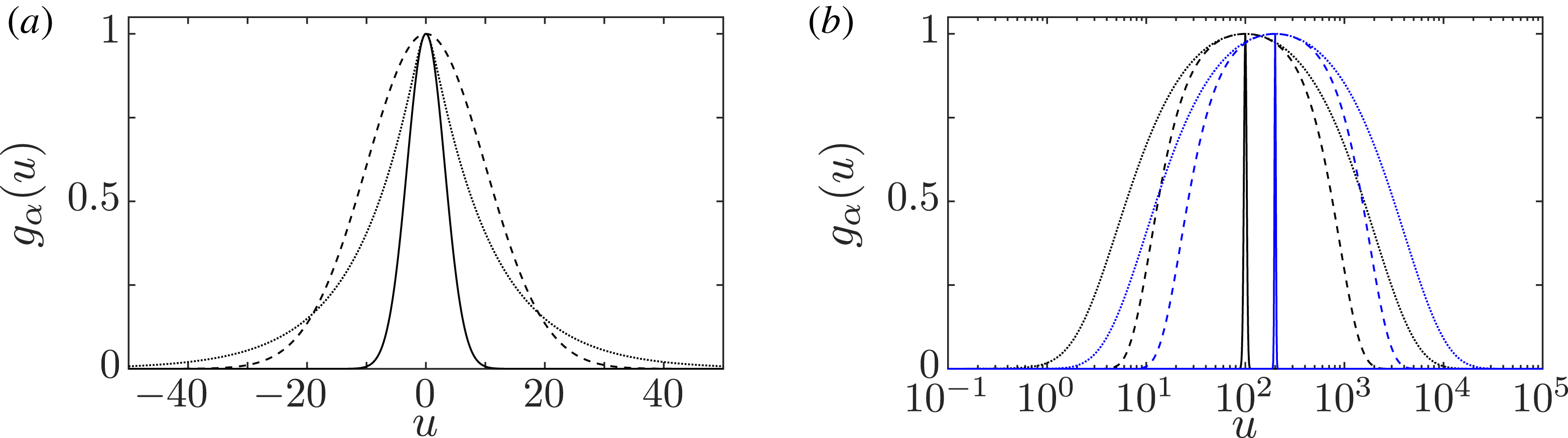
In figure 2 we plot the Gaussian (solid and dashed) and Jüttner (dotted) distributions for $\unicode[STIX]{x1D70C}_{\unicode[STIX]{x1D6FC}}=0.1$ . In (a) we choose $u_{\unicode[STIX]{x1D6FC}}=0$ for which the two expressions for the Gaussian distribution given by equations (3.3) and (3.4) coincide: $u_{\text{th}}^{2}=1/\unicode[STIX]{x1D70C}_{\unicode[STIX]{x1D6FC}}$ (solid) and $u_{\text{th}}^{2}=1/\unicode[STIX]{x1D70C}_{\unicode[STIX]{x1D6FC}}^{2}$ (dashed); and the Jüttner distribution (3.1) is given by the dotted curve. Comparison of the three cases shows that for small $|u|$ the width of the Jüttner distribution is intermediate between a Gaussian with $u_{\text{th}\unicode[STIX]{x1D6FC}}^{2}=1/\unicode[STIX]{x1D70C}_{\unicode[STIX]{x1D6FC}}$ and a Gaussian with $u_{\text{th}\unicode[STIX]{x1D6FC}}^{2}=1/\unicode[STIX]{x1D70C}_{\unicode[STIX]{x1D6FC}}^{2}$ , with the Jüttner distribution having much broader wings at larger $|u|$ . The number density is proportional to the area under the curve, $\propto \unicode[STIX]{x1D6FE}_{\unicode[STIX]{x1D6FC}}$ . The change when streaming is included is shown in (b) for $u_{\text{th}}^{2}=1/\unicode[STIX]{x1D70C}_{\unicode[STIX]{x1D6FC}}$ with $u_{\unicode[STIX]{x1D6FC}}=100$ (black curves) and 200 (blue curves). The solid curves show plots of the Gaussian distribution as given by (3.3) and the dashed curves show the form given by (3.4). The corresponding plots for the Jüttner distribution are given by the dotted curves. It is clear that the Lorentz-transformed Gaussian distribution (3.4) is much broader, with its width increasing as $u_{\unicode[STIX]{x1D6FC}}$ increases, whereas the width of the shifted Gaussian (3.3) is independent of $u_{\unicode[STIX]{x1D6FC}}$ . Below the peak at $u=u_{\unicode[STIX]{x1D6FC}}$ , the positive slope of the Jüttner distribution is much smaller than for either Gaussian, and above the peak the Jüttner distribution decreases much more slowly with $u$ than for either Gaussian. The width of the Lorentz-transformed Gaussian remains comparable to that of the Jüttner distribution when plotted as a function of the logarithm of $u=\unicode[STIX]{x1D6FE}\unicode[STIX]{x1D6FD}$ .

The streaming Gaussian distribution (3.3) is a poor approximation to a streaming Jüttner distribution for $\unicode[STIX]{x1D70C}_{\unicode[STIX]{x1D6FC}}\ll 1$ . In particular the slope of the distribution, $\text{d}g_{\unicode[STIX]{x1D6FC}}(u)/\text{d}u$ , for either Gaussian distribution is a poor approximation to the slope for the Jüttner distribution. This slope is directly relevant to a beam-driven instability, suggesting that the growth rate for a Jüttner distribution is poorly approximated by a streaming Gaussian model.

Figure 2.

Plots of Gaussian distribution as given by (3.3) (solid) and as given by (3.4) (dashed), and Jüttner distribution as given by (3.1) (dotted) as a function of $u=\unicode[STIX]{x1D6FE}\unicode[STIX]{x1D6FD}$ for $\unicode[STIX]{x1D70C}_{\unicode[STIX]{x1D6FC}}=0.1$ . (a)  $u_{\unicode[STIX]{x1D6FC}}=\unicode[STIX]{x1D6FE}_{\unicode[STIX]{x1D6FC}}\unicode[STIX]{x1D6FD}_{\unicode[STIX]{x1D6FC}}=0$ , with $u_{\text{th}}^{2}=1/\unicode[STIX]{x1D70C}_{\unicode[STIX]{x1D6FC}}$ (solid) and $u_{\text{th}}^{2}=1/\unicode[STIX]{x1D70C}_{\unicode[STIX]{x1D6FC}}^{2}$ (dashed). (b)  $u_{\text{th}}^{2}=1/\unicode[STIX]{x1D70C}_{\unicode[STIX]{x1D6FC}}$ with $u_{\unicode[STIX]{x1D6FC}}=100$ (black) and 200 (blue). The amplitude is in each case normalized to unity; the number density in each distribution is proportional to the area under the curve.

We suggest that the choice of a relativistically streaming Gaussian distribution (3.3) is made primarily for mathematical convenience. The choice (3.3) applies only in a specific frame, in the sense that it does not retain its form under a Lorentz transformation.

Another choice of (non-streaming) distribution function, made primarily for mathematical convenience, is of the form $g(u)\propto (u_{1}^{2}-u^{2})^{N}$ , for $u^{2}<u_{1}^{2}$ and $g(u)=0$ for $u^{2}>u_{1}^{2}$ , where $u_{1}$ is a constant, with the cases $n=0,1,2$ referred to as water-bag (Arons & Barnard Reference Arons and Barnard1986), hard-bell and soft-bell (Gedalin et al. Reference Gedalin, Melrose and Gruman1998; Melrose & Gedalin Reference Melrose and Gedalin1999) distributions, respectively. Applying a Lorentz transformation gives $g^{\prime }(u^{\prime })=g(u)$ with $u=\unicode[STIX]{x1D6FE}_{\unicode[STIX]{x1D6FC}}\unicode[STIX]{x1D6FE}^{\prime }(\unicode[STIX]{x1D6FD}^{\prime }-\unicode[STIX]{x1D6FD}_{\unicode[STIX]{x1D6FC}})$ . The range $-u_{1}<u<u_{1}$ in ${\mathcal{K}}$ transforms into $u_{1-}^{\prime }<u^{\prime }<u_{1+}^{\prime }$ in ${\mathcal{K}}^{\prime }$ , with $u_{1\pm }^{\prime }=\unicode[STIX]{x1D6FE}_{\unicode[STIX]{x1D6FC}}\unicode[STIX]{x1D6FE}_{1}(\pm \unicode[STIX]{x1D6FD}_{1}+\unicode[STIX]{x1D6FD}_{\unicode[STIX]{x1D6FC}})$ implying that the range $2u_{1}$ in ${\mathcal{K}}$ broadens to $u_{1+}^{\prime }-u_{1-}^{\prime }=\unicode[STIX]{x1D6FE}_{\unicode[STIX]{x1D6FC}}2u_{1}$ in ${\mathcal{K}}^{\prime }$ . In the highly relativistic case, $\unicode[STIX]{x1D6FE}_{\unicode[STIX]{x1D6FC}}\gg \unicode[STIX]{x1D6FE}_{1}\gg 1$ , these limits become $u_{1-}^{\prime }\approx -(\unicode[STIX]{x1D6FE}_{1}^{2}-\unicode[STIX]{x1D6FE}_{\unicode[STIX]{x1D6FC}}^{2})/2\unicode[STIX]{x1D6FE}_{1}\unicode[STIX]{x1D6FE}_{\unicode[STIX]{x1D6FC}}$ , $u_{1+}^{\prime }\approx \unicode[STIX]{x1D6FE}_{\unicode[STIX]{x1D6FC}}\unicode[STIX]{x1D6FE}_{1}$ . This much larger range in ${\mathcal{K}}^{\prime }$ implies that the number density in ${\mathcal{K}}^{\prime }$ is higher than that in ${\mathcal{K}}$ , by the same factor, $n^{\prime }/n=\unicode[STIX]{x1D6FE}_{\unicode[STIX]{x1D6FC}}$ , as is obvious in the case $N=0$ , where $g^{\prime }(u^{\prime })=g(u)$ is a constant, and is easily shown for $N>0$ . The parameter $\unicode[STIX]{x1D6FE}_{1}$ may be interpreted in terms of $\langle \unicode[STIX]{x1D6FE}\rangle _{\unicode[STIX]{x1D6FC}}$ , with $\unicode[STIX]{x1D6FE}_{1}=2\langle \unicode[STIX]{x1D6FE}\rangle _{\unicode[STIX]{x1D6FC}}$ for $N=0$ and $\unicode[STIX]{x1D6FE}_{1}=8\langle \unicode[STIX]{x1D6FE}\rangle _{\unicode[STIX]{x1D6FC}}/3$ for $N=1$ .

We adopt the view that the default choice for a relativistic distribution is a Jüttner distribution in the rest frame of the plasma, and that the default choice for a relativistically streaming distribution is that obtained by applying a Lorentz transformation to the distribution function in the rest frame. The fact that the resulting streaming distribution is very much broader than the rest-frame distribution is a characteristic feature, which applies to but is not restricted to a Jüttner distribution.

3.3 Examples of relativistically streaming distributions

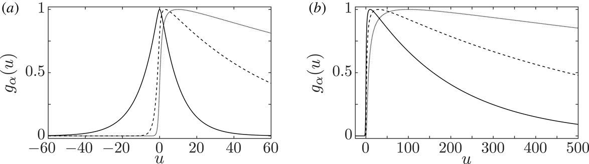
In figure 3 we plot the distribution function (3.1) for $\unicode[STIX]{x1D70C}_{\unicode[STIX]{x1D6FC}}=0.1$ , and for several values of $u_{\unicode[STIX]{x1D6FC}}=\unicode[STIX]{x1D6FE}_{\unicode[STIX]{x1D6FC}}\unicode[STIX]{x1D6FD}_{\unicode[STIX]{x1D6FC}}$ . In (a) is shown a non-streaming distribution, $\unicode[STIX]{x1D6FD}_{\unicode[STIX]{x1D6FC}}=0$ (solid), and two streaming distributions, $\unicode[STIX]{x1D6FE}_{\unicode[STIX]{x1D6FC}}\unicode[STIX]{x1D6FD}_{\unicode[STIX]{x1D6FC}}=3$ (dashed) and $\unicode[STIX]{x1D6FE}_{\unicode[STIX]{x1D6FC}}\unicode[STIX]{x1D6FD}_{\unicode[STIX]{x1D6FC}}=10$ (dotted). The non-streaming distribution is symmetric about the origin, $u=0$ ; a slight asymmetry develops for a small streaming speed, and for $\unicode[STIX]{x1D6FE}_{\unicode[STIX]{x1D6FC}}\unicode[STIX]{x1D6FD}_{\unicode[STIX]{x1D6FC}}\approx 1/\unicode[STIX]{x1D70C}_{\unicode[STIX]{x1D6FC}}\approx \langle \unicode[STIX]{x1D6FE}\rangle _{\unicode[STIX]{x1D6FC}}$ , for $\unicode[STIX]{x1D70C}_{\unicode[STIX]{x1D6FC}}\ll 1$ , the asymmetry is substantial. In the case $u_{\unicode[STIX]{x1D6FC}}\approx \langle \unicode[STIX]{x1D6FE}\rangle _{\unicode[STIX]{x1D6FC}}\approx 10$ the distribution function is almost negligible for $u<0$ , and increases with increasing $u>0$ to a maximum near $u=u_{\unicode[STIX]{x1D6FC}}\approx 10$ , and then decreases slowly for $u\gg u_{\unicode[STIX]{x1D6FC}}$ . In figure 3(b) we show the cases $u_{\unicode[STIX]{x1D6FC}}=10$ (solid), 30 (dashed), 100 (dotted) on a larger scale. In each case the distribution function has a maximum at $u=u_{\unicode[STIX]{x1D6FC}}$ . Note that the normalization in figure 3 is chosen to show the relative shapes of the distributions: each is normalized so that its maximum is unity. The number density in each case is proportional to the area under the curve, which is $\propto \unicode[STIX]{x1D6FE}_{\unicode[STIX]{x1D6FC}}$ for a streaming Jüttner distribution; with normalization to a fixed number density the maxima would be $\propto 1/\unicode[STIX]{x1D6FE}_{\unicode[STIX]{x1D6FC}}$ .Footnote ²

Figure 3.

A non-streaming and streaming Jüttner distributions are plotted as a function of $u=\unicode[STIX]{x1D6FE}\unicode[STIX]{x1D6FD}$ for $\unicode[STIX]{x1D70C}_{\unicode[STIX]{x1D6FC}}=0.1$ . (a)  $u_{\unicode[STIX]{x1D6FC}}=\unicode[STIX]{x1D6FE}_{\unicode[STIX]{x1D6FC}}\unicode[STIX]{x1D6FD}_{\unicode[STIX]{x1D6FC}}=0$ (solid), 3 (dashed), 10 (dotted). (b)  $u_{\unicode[STIX]{x1D6FC}}=10$ (solid), 30 (dashed), 100 (dotted). The amplitude is in each case normalized to unity; the number density in each distribution is proportional to the area under the curve.

3.4 Highly relativistically streaming Jüttner distribution

An analytic approximation to a highly relativistically streaming Jüttner distribution, with $\unicode[STIX]{x1D70C}_{\unicode[STIX]{x1D6FC}}\ll 1$ and $\unicode[STIX]{x1D70C}_{\unicode[STIX]{x1D6FC}}\unicode[STIX]{x1D6FE}_{\unicode[STIX]{x1D6FC}}\gg 1$ , may be found by expanding the exponential factor in (3.1) in powers of $1/\unicode[STIX]{x1D6FE}_{\unicode[STIX]{x1D6FC}}\ll 1$ and $1/\unicode[STIX]{x1D6FE}\ll 1$ ,

(3.5) $$\begin{eqnarray}\exp [-\unicode[STIX]{x1D70C}_{\unicode[STIX]{x1D6FC}}\unicode[STIX]{x1D6FE}_{\unicode[STIX]{x1D6FC}}\unicode[STIX]{x1D6FE}(1-\unicode[STIX]{x1D6FD}_{\unicode[STIX]{x1D6FC}}\unicode[STIX]{x1D6FD})]\approx \left\{\begin{array}{@{}ll@{}}\displaystyle \exp \left[-\unicode[STIX]{x1D70C}_{\unicode[STIX]{x1D6FC}}\frac{(\unicode[STIX]{x1D6FE}-\unicode[STIX]{x1D6FE}_{\unicode[STIX]{x1D6FC}})^{2}}{2\unicode[STIX]{x1D6FE}_{\unicode[STIX]{x1D6FC}}\unicode[STIX]{x1D6FE}}-\unicode[STIX]{x1D70C}_{\unicode[STIX]{x1D6FC}}\right]\quad & \text{for }\unicode[STIX]{x1D6FD}>0,\\ 0\quad & \text{for }\unicode[STIX]{x1D6FD}<0.\end{array}\right.\end{eqnarray}$$

This gives

(3.6) $$\begin{eqnarray}g_{\unicode[STIX]{x1D6FC}}(u)=\frac{1}{2}n_{\unicode[STIX]{x1D6FC}}\unicode[STIX]{x1D70C}_{\unicode[STIX]{x1D6FC}}\exp \left[-\unicode[STIX]{x1D70C}_{\unicode[STIX]{x1D6FC}}\frac{(\unicode[STIX]{x1D6FE}-\unicode[STIX]{x1D6FE}_{\unicode[STIX]{x1D6FC}})^{2}}{2\unicode[STIX]{x1D6FE}\unicode[STIX]{x1D6FE}_{\unicode[STIX]{x1D6FC}}}\right]H(u),\end{eqnarray}$$

where $H(u)=1$ for $u>0$ and $H(u)=0$ for $u<0$ is the step function, and we use $1/K_{1}(\unicode[STIX]{x1D70C}_{\unicode[STIX]{x1D6FC}})=\unicode[STIX]{x1D70C}_{\unicode[STIX]{x1D6FC}}+O(\unicode[STIX]{x1D70C}_{\unicode[STIX]{x1D6FC}}^{3})$ for $\unicode[STIX]{x1D70C}_{\unicode[STIX]{x1D6FC}}\ll 1$ .

Figure 4.

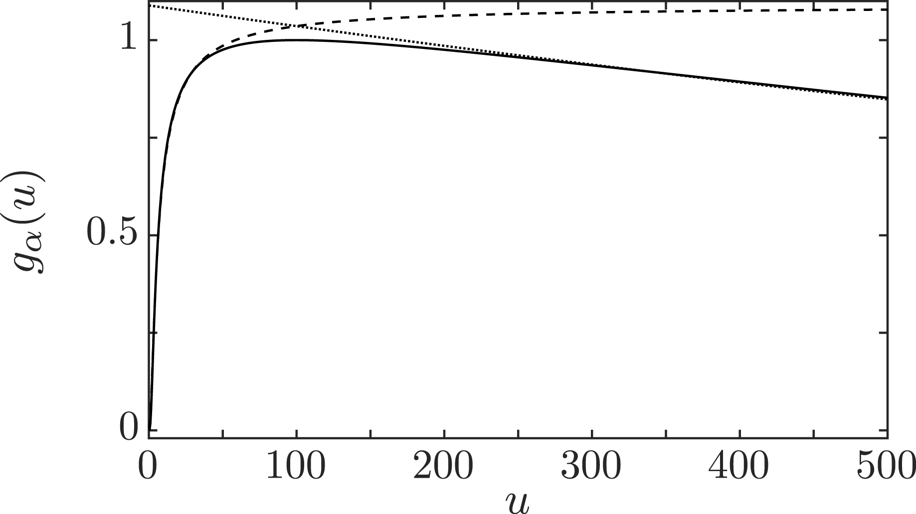
Comparison of the approximate forms (3.7) and the exact form (3.1) of a Jüttner distribution with $\unicode[STIX]{x1D70C}_{\unicode[STIX]{x1D6FC}}=0.1$ and $u_{\unicode[STIX]{x1D6FC}}=100$ . The solid curve is the exact distribution, the dashed curve is the approximation for $\unicode[STIX]{x1D6FE}\ll \unicode[STIX]{x1D6FE}_{\unicode[STIX]{x1D6FC}}$ and the dotted curve is the approximation for $\unicode[STIX]{x1D6FE}\gg \unicode[STIX]{x1D6FE}_{\unicode[STIX]{x1D6FC}}$ . Normalization as in figures 2 and 3.

The approximation (3.5) gives approximate forms for the highly relativistically streaming Jüttner distribution function below and above the peak of the distribution at $\unicode[STIX]{x1D6FE}=\unicode[STIX]{x1D6FE}_{\unicode[STIX]{x1D6FC}}$ :

(3.7) $$\begin{eqnarray}g_{\unicode[STIX]{x1D6FC}}(u)\approx \frac{1}{2}n_{\unicode[STIX]{x1D6FC}}\unicode[STIX]{x1D70C}_{\unicode[STIX]{x1D6FC}}\left\{\begin{array}{@{}ll@{}}\exp (-\unicode[STIX]{x1D70C}_{\unicode[STIX]{x1D6FC}}\unicode[STIX]{x1D6FE}_{\unicode[STIX]{x1D6FC}}/2\unicode[STIX]{x1D6FE})\quad & \text{for }\unicode[STIX]{x1D6FE}\ll \unicode[STIX]{x1D6FE}_{\unicode[STIX]{x1D6FC}},\\ \exp (-\unicode[STIX]{x1D70C}_{\unicode[STIX]{x1D6FC}}\unicode[STIX]{x1D6FE}/2\unicode[STIX]{x1D6FE}_{\unicode[STIX]{x1D6FC}})\quad & \text{for }\unicode[STIX]{x1D6FE}\gg \unicode[STIX]{x1D6FE}_{\unicode[STIX]{x1D6FC}}.\end{array}\right.\end{eqnarray}$$

The exact form and the two approximate forms (3.7) are compared in figure 4. The approximation for $\unicode[STIX]{x1D6FE}\ll \unicode[STIX]{x1D6FE}_{\unicode[STIX]{x1D6FC}}$ implies a positive slope $\text{d}g_{\unicode[STIX]{x1D6FC}}(u)/\text{d}u\approx (\unicode[STIX]{x1D70C}_{\unicode[STIX]{x1D6FC}}\unicode[STIX]{x1D6FE}_{\unicode[STIX]{x1D6FC}}/2\unicode[STIX]{x1D6FE}^{2})g_{\unicode[STIX]{x1D6FC}}(u)$ . The approximation for $\unicode[STIX]{x1D6FE}\gg \unicode[STIX]{x1D6FE}_{\unicode[STIX]{x1D6FC}}$ implies that a relativistically streaming Jüttner distribution asymptotes to the same form as a non-streaming Jüttner distribution, with $\unicode[STIX]{x1D70C}_{\unicode[STIX]{x1D6FC}}$ replaced by $\unicode[STIX]{x1D70C}_{\unicode[STIX]{x1D6FC}}/2\unicode[STIX]{x1D6FE}_{\unicode[STIX]{x1D6FC}}$ in the exponent.

For comparison we consider the same highly relativistic approximation to the Lorentz-transformed Gaussian distribution (3.4). In place of (3.7), this gives

(3.8) $$\begin{eqnarray}g_{\unicode[STIX]{x1D6FC}}(u)\propto \left\{\begin{array}{@{}ll@{}}\exp (-\unicode[STIX]{x1D6FE}_{\unicode[STIX]{x1D6FC}}^{2}/8\unicode[STIX]{x1D6FE}^{2}u_{\text{t h}}^{2})\quad & \text{for }\unicode[STIX]{x1D6FE}^{2}\ll \unicode[STIX]{x1D6FE}_{\unicode[STIX]{x1D6FC}}^{2},\\ \exp (-\unicode[STIX]{x1D6FE}^{2}/8\unicode[STIX]{x1D6FE}_{\unicode[STIX]{x1D6FC}}^{2}u_{\text{th}}^{2})\quad & \text{for }\unicode[STIX]{x1D6FE}^{2}\gg \unicode[STIX]{x1D6FE}_{\unicode[STIX]{x1D6FC}}^{2}.\end{array}\right.\end{eqnarray}$$

The distribution (3.8) is very much broader than the conventional form (3.3) for a relativistically streaming Gaussian distribution, as is evident by the way in which they fall off for $\unicode[STIX]{x1D6FE}^{2}\gg \unicode[STIX]{x1D6FE}_{\unicode[STIX]{x1D6FC}}^{2}$ : specifically $\propto \exp (-\unicode[STIX]{x1D6FE}^{2}/2u_{\text{th}}^{2})$ and $\propto \exp (-\unicode[STIX]{x1D6FE}^{2}/8\unicode[STIX]{x1D6FE}_{\unicode[STIX]{x1D6FC}}^{2}u_{\text{th}}^{2})$ , respectively.

4.1 Counter-streaming distributions

An idealized counter-streaming distribution consists of two streaming Jüttner distributions, $\unicode[STIX]{x1D6FC}=\pm$ , with $\bar{n}_{\pm }=\bar{n}/2$ , $|\unicode[STIX]{x1D6FD}_{\pm }|=\bar{\unicode[STIX]{x1D6FD}}$ , and the same temperature $\unicode[STIX]{x1D70C}_{\pm }=\unicode[STIX]{x1D70C}\approx 1/\langle \unicode[STIX]{x1D6FE}\rangle \ll 1$ . The resulting distribution function is

(4.1a,b ) $$\begin{eqnarray}g_{\text{cs}}(u)=\frac{\bar{n}F(u)}{2\bar{\unicode[STIX]{x1D6FE}}K_{1}(\unicode[STIX]{x1D70C})},\quad F(u)=\exp [-\unicode[STIX]{x1D70C}\bar{\unicode[STIX]{x1D6FE}}\unicode[STIX]{x1D6FE}(1-\unicode[STIX]{x1D6FD}\bar{\unicode[STIX]{x1D6FD}})]+\exp [-\unicode[STIX]{x1D70C}\bar{\unicode[STIX]{x1D6FE}}\unicode[STIX]{x1D6FE}(1+\unicode[STIX]{x1D6FD}\bar{\unicode[STIX]{x1D6FD}})].\end{eqnarray}$$

We first discuss how the distribution changes as the speed $\bar{u}=\bar{\unicode[STIX]{x1D6FE}}\bar{\unicode[STIX]{x1D6FD}}$ increases from zero to $\bar{\unicode[STIX]{x1D6FE}}\gtrsim 1/\unicode[STIX]{x1D70C}\gg 1$ . We then transform to the frame where one of the distributions is at rest and consider the highly relativistic case.

Figure 5.

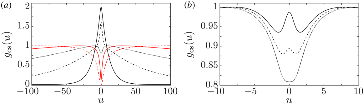
The sum of two counter-streaming Jüttner distributions is plotted as a function of $u=\unicode[STIX]{x1D6FE}\unicode[STIX]{x1D6FD}$ for $\unicode[STIX]{x1D70C}=0.1$ . (a) For $\bar{u}=\bar{\unicode[STIX]{x1D6FE}}\bar{\unicode[STIX]{x1D6FD}}=0$ (black solid), 3 (black dashed), 10 (black dotted), 30 (red solid), 100 (red dashed). (b) For $\bar{u}=8$ (solid), 9 (dashed), 10 (dotted) showing the disappearance of the peak at $u=0$ . The normalization of both distributions is chosen such that its maximum, at $u=\pm \bar{u}$ , is unity.

For $\bar{u}=0$ the two distributions are identical, and their sum is a single Jüttner distribution, corresponding to the solid black curve in figure 5(a). As shown in figure 5, the curves move apart with increasing $\bar{u}$ , becoming almost completely separated for $\bar{u}\gg 10$ . This ‘separation condition’ is important in estimating the conditions under which the combined distribution can be interpreted as a beam propagating through a background distribution. The separation condition was discussed by Lazar, Stockem & Schlickeiser (Reference Lazar, Stockem and Schlickeiser2010), who considered the 3-D counterpart, but this difference is unimportant here. Separation occurs for $\bar{\unicode[STIX]{x1D6FE}}\bar{\unicode[STIX]{x1D6FD}}^{2}>1/\unicode[STIX]{x1D70C}$ , as shown in figure 5(b). For $\{\bar{u},\langle \unicode[STIX]{x1D6FE}\rangle \}\gg 1$ we may write this separation condition as $\bar{u}/\langle \unicode[STIX]{x1D6FE}\rangle \gtrsim 1$ .

4.1.1 Transformation to rest frame of one beam

The properties of the counter-streaming distribution are useful in discussing the weak-beam model. The idea is that by transforming to the frame in which the backward-propagating distribution is at rest, the backward-propagating distribution is reinterpreted as the background distribution, with the forward-propagating distribution being regarded as the beam. The weak-beam case follows by multiplying the latter distribution by the ratio of the beam to background densities. The relative speed between the two distributions becomes the beam speed

(4.2a-c ) $$\begin{eqnarray}\unicode[STIX]{x1D6FD}_{\text{b}}=\frac{2\bar{\unicode[STIX]{x1D6FD}}}{1+\bar{\unicode[STIX]{x1D6FD}}^{2}},\quad \unicode[STIX]{x1D6FE}_{\text{b}}=(1+\bar{\unicode[STIX]{x1D6FD}}^{2})\bar{\unicode[STIX]{x1D6FE}}^{2},\quad u_{\text{b}}=\unicode[STIX]{x1D6FE}_{\text{b}}\unicode[STIX]{x1D6FD}_{\text{b}}=2\bar{\unicode[STIX]{x1D6FD}}\bar{\unicode[STIX]{x1D6FE}}^{2}.\end{eqnarray}$$

Let a quantity in the frame in which the backward-propagating beam is at rest be denoted by a prime. Then in (4.1) one has

(4.3a,b ) $$\begin{eqnarray}\unicode[STIX]{x1D6FE}\bar{\unicode[STIX]{x1D6FE}}(1+\unicode[STIX]{x1D6FD}\bar{\unicode[STIX]{x1D6FD}})=\unicode[STIX]{x1D6FE}^{\prime },\quad \unicode[STIX]{x1D6FE}\bar{\unicode[STIX]{x1D6FE}}(1-\unicode[STIX]{x1D6FD}\bar{\unicode[STIX]{x1D6FD}})=\unicode[STIX]{x1D6FE}^{\prime }\unicode[STIX]{x1D6FE}_{\text{b}}(1-\unicode[STIX]{x1D6FD}^{\prime }\unicode[STIX]{x1D6FD}_{\text{b}}).\end{eqnarray}$$

Let $n_{0}$ be the number density of either beam in the rest frame of that beam. Using the fact that $g_{\text{cs}}^{\prime }(u^{\prime })=g_{\text{cs}}(u)$ is an invariant, in the primed frame equation (4.1) becomes

(4.4) $$\begin{eqnarray}g_{\text{cs}}^{\prime }(u^{\prime })=\frac{n_{0}}{2K_{1}(\unicode[STIX]{x1D70C})}\left\{\exp (-\unicode[STIX]{x1D70C}\unicode[STIX]{x1D6FE}^{\prime })+\frac{n_{\text{b}}}{\unicode[STIX]{x1D6FE}_{\text{b}}n_{0}}\exp [-\unicode[STIX]{x1D70C}\unicode[STIX]{x1D6FE}^{\prime }\unicode[STIX]{x1D6FE}_{\text{b}}(1-\unicode[STIX]{x1D6FD}^{\prime }\unicode[STIX]{x1D6FD}_{\text{b}})]\right\},\end{eqnarray}$$

with $n_{\text{b}}=\unicode[STIX]{x1D6FE}_{\text{b}}n_{0}$ in this case. Equation (4.4), with primes omitted, becomes a weak-beam model for $n_{\text{b}}/\unicode[STIX]{x1D6FE}_{\text{b}}n_{0}\ll 1$ .

4.2 Separation condition

The condition $\bar{u}\approx \bar{\unicode[STIX]{x1D6FE}}\gtrsim \langle \unicode[STIX]{x1D6FE}\rangle$ for two identical counter-streaming Jüttner distributions to become well separated, transforms into $\unicode[STIX]{x1D6FE}_{\text{b}}\gtrsim 2\langle \unicode[STIX]{x1D6FE}\rangle ^{2}$ in the frame in which one of the beams is at rest. The Lorentz transformation to the new frame makes this separation condition appear to be more extreme than in the counter-streaming frame. This separation condition is a direct result of the Lorentz transformation, and is not specific to Jüttner distributions, as may be seen by considering counter-streaming distributions that are Gaussian in their respective rest frames.

In contrast, for counter-streaming Gaussian distributions of the form given by (3.3), with $\unicode[STIX]{x1D6FC}=\pm$ , $u_{\pm }=\pm \bar{u}$ , $n_{\pm }=\bar{n}/2$ and the same $u_{\text{th}}$ , the separation condition is closely analogous to that for the corresponding non-relativistic counterpart, in which a Gaussian distribution is equivalent to a Maxwellian distribution. The two distributions become well separated when the streaming speeds exceed the thermal spreads, corresponding to $\bar{u}\gtrsim u_{\text{th}}$ . This condition transforms into $\unicode[STIX]{x1D6FE}_{\text{b}}\gtrsim 2u_{\text{th}}^{2}$ , which is equivalent to $\unicode[STIX]{x1D6FE}_{\text{b}}\gtrsim 2\langle \unicode[STIX]{x1D6FE}\rangle ^{2}$ for Jüttner distributions.

4.3 Weak-beam model

In a weak-beam model there are only two components, which we denote by $\unicode[STIX]{x1D6FC}=0,b$ , where $\unicode[STIX]{x1D6FC}=0$ refers to the background and $\unicode[STIX]{x1D6FC}=b$ refers to the beam. The frame of interest is identified as the rest frame of the background in this case. The distribution function is then $g(u)=g_{0}(u)+g_{\text{b}}(u)$ ,

(4.5) $$\begin{eqnarray}g(u)=n_{0}\left[\frac{\text{e}^{-\unicode[STIX]{x1D70C}_{0}\unicode[STIX]{x1D6FE}}}{2K_{1}(\unicode[STIX]{x1D70C}_{0})}+\unicode[STIX]{x1D700}_{n}\frac{\text{e}^{-\unicode[STIX]{x1D70C}_{\text{b}}\unicode[STIX]{x1D6FE}_{\text{b}}\unicode[STIX]{x1D6FE}(1-\unicode[STIX]{x1D6FD}\unicode[STIX]{x1D6FD}_{\text{b}})}}{2K_{1}(\unicode[STIX]{x1D70C}_{\text{b}})}\right],\end{eqnarray}$$

with $\unicode[STIX]{x1D700}_{n}=n_{\text{b}}/\unicode[STIX]{x1D6FE}_{\text{b}}n_{0}\ll 1$ , where the first term is $g_{0}(u)$ and the second term is $g_{\text{b}}(u)$ . For $\unicode[STIX]{x1D70C}_{0}=\unicode[STIX]{x1D70C}_{\text{b}}=\unicode[STIX]{x1D70C}$ , this result also follows from (4.4) by omitting the primes and allowing arbitrary $n_{\text{b}}/\unicode[STIX]{x1D6FE}_{\text{b}}n_{0}\ll 1$ .

A conventional approach to treating wave dispersion in this case is based on an expansion in $\unicode[STIX]{x1D700}_{n}\ll 1$ . To zeroth order the beam is ignored, such that the wave dispersion is determined by the background plasma alone. To first order the beam contributes a correction to the frequency, which includes both imaginary and real parts, with the former determining the growth rate of any beam-driven instability. In the case of a maser instability, due to negative absorption, growth requires $\text{d}g(u)/\text{d}u>0$ at the resonant frequency, determined by $u=\unicode[STIX]{x1D6FE}\unicode[STIX]{x1D6FD}=\unicode[STIX]{x1D6FE}_{\unicode[STIX]{x1D719}}z$ .

Figure 6.

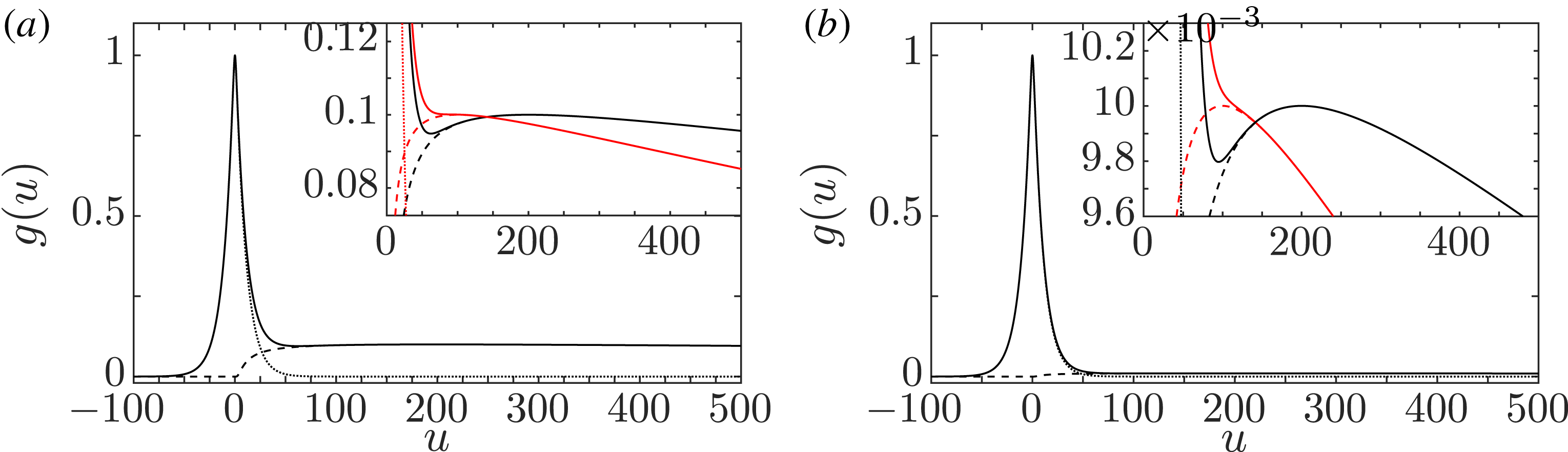
Weak-beam distribution functions with $\unicode[STIX]{x1D70C}=0.1$ for (a) $\unicode[STIX]{x1D700}_{n}=0.1$ and (b) $\unicode[STIX]{x1D700}_{n}=0.01$ , and for $u_{\text{b}}=200$ (black curves). In the inset we show a zoomed version of each plot and also include a plot for $u_{\text{b}}=100$ (red curves). The solid curve corresponds to $g(u)=g_{0}(u)+g_{\text{b}}(u)$ , the dashed and dotted curves are the background and beam distributions, respectively.

In figure 6 we plot the weak-beam distribution function (4.5) for $\unicode[STIX]{x1D70C}=0.1$ , for two values of $\unicode[STIX]{x1D700}_{n}=0.1$ on the left and $0.01$ on the right, and for $u_{\text{b}}=100,200$ . For $\unicode[STIX]{x1D700}_{n}=0.1$ the minimum and maximum (at $u=u_{\text{b}}$ ) in $g(u)$ that would be present in the absence of the background have almost disappeared for $u_{\text{b}}=100$ , but are still present for $u_{\text{b}}=200$ . For $\unicode[STIX]{x1D700}_{n}=0.01$ the minimum and maximum for $u_{\text{b}}=100$ are nearly smoothed out.

Figure 7.

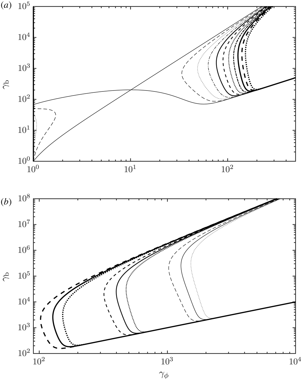
Contour plots of $\text{d}g(u)/\text{d}\unicode[STIX]{x1D6FD}|_{\unicode[STIX]{x1D6FD}=z}=0$ over $\unicode[STIX]{x1D6FE}_{\unicode[STIX]{x1D719}}$ and $\unicode[STIX]{x1D6FE}_{\text{b}}$ . (a) For $\unicode[STIX]{x1D70C}_{0}=0.1$ , $\unicode[STIX]{x1D700}_{\unicode[STIX]{x1D70C}}=1$ , with $\unicode[STIX]{x1D700}_{n}$ sampled logarithmically from $10^{-5}$ (thick dotted) to $1$ (thin solid). (b) For $\unicode[STIX]{x1D700}_{\unicode[STIX]{x1D70C}}=1$ , $\unicode[STIX]{x1D70C}_{0}=0.1$ (thick), 0.032 (medium), 0.01 (thin) with $\unicode[STIX]{x1D700}_{n}=10^{-5}$ (dotted), $10^{-4}$ (solid) and $10^{-3}$ (dashed).

For $\unicode[STIX]{x1D700}_{n}\neq 1$ the separation condition $\unicode[STIX]{x1D6FE}_{\text{b}}\gtrsim 2\langle \unicode[STIX]{x1D6FE}\rangle _{0}^{2}$ is modified, where $\langle \cdots \rangle _{0}$ indicates average over the background distribution. In figure 7 we show contour plots of $\text{d}g(u)/\text{d}\unicode[STIX]{x1D6FD}|_{\unicode[STIX]{x1D6FD}=z}=0$ over $\unicode[STIX]{x1D6FE}_{\unicode[STIX]{x1D719}}$ and $\unicode[STIX]{x1D6FE}_{\text{b}}$ for various values of $\unicode[STIX]{x1D70C}_{0}$ and $\unicode[STIX]{x1D700}_{n}$ . (a) For $\unicode[STIX]{x1D70C}_{0}=0.1$ , $\unicode[STIX]{x1D700}_{\unicode[STIX]{x1D70C}}=\unicode[STIX]{x1D70C}_{\text{b}}/\unicode[STIX]{x1D70C}_{0}=1$ and $\unicode[STIX]{x1D700}_{n}$ sampled logarithmically from $10^{-5}$ (thick dotted) to $1$ (thin solid). The thin solid curve corresponding to $\unicode[STIX]{x1D700}_{n}=1$ is a separatrix with the solution $\unicode[STIX]{x1D6FE}_{\unicode[STIX]{x1D719}}\approx 2\langle \unicode[STIX]{x1D6FE}\rangle _{0}^{2}$ denoting a saddle point at $(\unicode[STIX]{x1D6FE}_{\unicode[STIX]{x1D719}},\unicode[STIX]{x1D6FE}_{\text{b}})\approx (10,200)$ , for $\langle \unicode[STIX]{x1D6FE}\rangle _{0}\approx 1/\unicode[STIX]{x1D70C}_{0}=10$ . Solutions of $\text{d}g(u)/\text{d}\unicode[STIX]{x1D6FD}|_{\unicode[STIX]{x1D6FD}=z}=0$ lie in the two regions shown when $\unicode[STIX]{x1D700}_{n}<1$ and lie outside these regions for $\unicode[STIX]{x1D700}_{n}>1$ (which is not of interest here). For $3\unicode[STIX]{x1D70C}_{0}\lesssim \unicode[STIX]{x1D700}_{n}\leqslant 1$ the derivative of the distribution function has three peaks (and two troughs) for each $\unicode[STIX]{x1D6FE}_{\text{b}}$ over the range $\unicode[STIX]{x1D6FE}_{\text{b,min}}\lesssim \unicode[STIX]{x1D6FE}_{\text{b}}\lesssim 2\langle \unicode[STIX]{x1D6FE}\rangle _{0}^{2}$ , where

(4.6) $$\begin{eqnarray}\unicode[STIX]{x1D6FE}_{\text{b,min}}\approx 7.8(1/\unicode[STIX]{x1D700}_{n}\unicode[STIX]{x1D700}_{\unicode[STIX]{x1D70C}}\unicode[STIX]{x1D700}_{K})^{0.076}(1/\unicode[STIX]{x1D70C}_{0})^{1.07}\end{eqnarray}$$

is obtained numerically, with $\unicode[STIX]{x1D700}_{K}=K_{1}(\unicode[STIX]{x1D70C}_{0})/K_{1}(\unicode[STIX]{x1D70C}_{\text{b}})\approx \unicode[STIX]{x1D700}_{\unicode[STIX]{x1D70C}}$ for $\{\unicode[STIX]{x1D70C}_{0},\unicode[STIX]{x1D70C}_{\text{b}}\}\ll 1$ . For $\unicode[STIX]{x1D700}_{n}\lesssim 3\unicode[STIX]{x1D70C}_{0}$ , for each $\unicode[STIX]{x1D6FE}_{\text{b}}$ the derivative always has a maximum at $\unicode[STIX]{x1D6FE}_{\unicode[STIX]{x1D719}}\approx 1$ (near the peak of the background) which lies on the vertical axis in figure 7(a), and for $\unicode[STIX]{x1D6FE}_{\text{b}}\gtrsim \unicode[STIX]{x1D6FE}_{\text{b,min}}$ a second peak is at $\unicode[STIX]{x1D6FE}_{\unicode[STIX]{x1D719}}\approx \unicode[STIX]{x1D6FE}_{\text{b}}$ (near the peak of the beam) which follows the lower branch of the separatrix: $\unicode[STIX]{x1D6FE}_{\text{b}}\approx \unicode[STIX]{x1D6FE}_{\unicode[STIX]{x1D719}}$ . The solution corresponding to the trough between these two peaks deviates from the lower branch of the separatrix at $\unicode[STIX]{x1D6FE}_{\text{b}}\approx \unicode[STIX]{x1D6FE}_{\text{b,min}}$ , rises sharply and then asymptotically approaches the upper branch of the separatrix: $\unicode[STIX]{x1D6FE}_{\text{b}}\approx (2/\unicode[STIX]{x1D700}_{\unicode[STIX]{x1D70C}})\unicode[STIX]{x1D6FE}_{\unicode[STIX]{x1D719}}^{2}$ . (b) For $\unicode[STIX]{x1D700}_{\unicode[STIX]{x1D70C}}=1$ , $\unicode[STIX]{x1D70C}_{0}=0.1$ (thick), 0.032 (medium), 0.01 (thin) with $\unicode[STIX]{x1D700}_{n}=10^{-5}$ (dotted), $10^{-4}$ (solid) and $10^{-3}$ (dashed). The asymptotic behaviour discussed is more readily evident here where we increase the range of $\unicode[STIX]{x1D6FE}_{\text{b}}$ and focus on the peak at $\unicode[STIX]{x1D6FE}_{\unicode[STIX]{x1D719}}\approx \unicode[STIX]{x1D6FE}_{\text{b}}$ and the trough of $\text{d}g(u)/\text{d}\unicode[STIX]{x1D6FD}|_{\unicode[STIX]{x1D6FD}=z}$ . The lower branch of the separatrix and the contour of the trough are given by

(4.7a,b ) $$\begin{eqnarray}\unicode[STIX]{x1D6FE}_{\text{b}}=\unicode[STIX]{x1D6FE}_{\unicode[STIX]{x1D719}}+\frac{\unicode[STIX]{x1D6FE}_{\unicode[STIX]{x1D719}}^{3}\text{e}^{-\unicode[STIX]{x1D70C}_{0}\unicode[STIX]{x1D6FE}_{\unicode[STIX]{x1D719}}}}{\unicode[STIX]{x1D700}_{n}\unicode[STIX]{x1D700}_{\unicode[STIX]{x1D70C}}\unicode[STIX]{x1D700}_{K}}\approx \unicode[STIX]{x1D6FE}_{\unicode[STIX]{x1D719}}\quad \text{and}\quad 1-\frac{\unicode[STIX]{x1D700}_{n}\unicode[STIX]{x1D700}_{\unicode[STIX]{x1D70C}}\unicode[STIX]{x1D700}_{K}\unicode[STIX]{x1D6FE}_{\text{b}}}{2\unicode[STIX]{x1D6FE}_{\unicode[STIX]{x1D719}}^{2}}\exp \left[\frac{\unicode[STIX]{x1D6FE}_{\unicode[STIX]{x1D719}}}{\langle \unicode[STIX]{x1D6FE}\rangle _{0}}\left(1-\frac{\unicode[STIX]{x1D700}_{\unicode[STIX]{x1D70C}}\unicode[STIX]{x1D6FE}_{\text{b}}}{2\unicode[STIX]{x1D6FE}_{\unicode[STIX]{x1D719}}^{2}}\right)\right]=0,\end{eqnarray}$$

respectively, where we assume $\{\unicode[STIX]{x1D6FE}_{\unicode[STIX]{x1D719}},\unicode[STIX]{x1D6FE}_{\text{b}}\}\gg 1$ . The background and the beam may be considered as separated if for $\unicode[STIX]{x1D700}_{n}\ll 1$ we have $\unicode[STIX]{x1D6FE}_{\text{b}}\gtrsim \unicode[STIX]{x1D6FE}_{\text{b,min}}$ with $\unicode[STIX]{x1D6FE}_{\text{b,min}}$ given by (4.6).

5.1 Transformation of $\unicode[STIX]{x1D6F1}_{ij}$

The specific forms for the non-zero components of $\unicode[STIX]{x1D6F1}_{ij}$ found in Part 1 are

(5.2) $$\begin{eqnarray}\left.\begin{array}{@{}c@{}}\displaystyle \unicode[STIX]{x1D6F1}_{11}=\unicode[STIX]{x1D6F1}_{22}=\frac{\unicode[STIX]{x1D714}_{\text{p}}^{2}}{\unicode[STIX]{x1D6FA}_{\text{e}}^{2}}\frac{\unicode[STIX]{x1D714}^{2}}{z^{2}}\langle \unicode[STIX]{x1D6FE}(z-\unicode[STIX]{x1D6FD})^{2}\rangle ,\quad \unicode[STIX]{x1D6F1}_{13}=\unicode[STIX]{x1D6F1}_{31}=\frac{\unicode[STIX]{x1D714}_{\text{p}}^{2}}{\unicode[STIX]{x1D6FA}_{\text{e}}^{2}}\frac{\unicode[STIX]{x1D714}^{2}\tan \unicode[STIX]{x1D703}}{z^{2}}\langle \unicode[STIX]{x1D6FE}\unicode[STIX]{x1D6FD}(z-\unicode[STIX]{x1D6FD})\rangle ,\\ \displaystyle \unicode[STIX]{x1D6F1}_{33}=-\unicode[STIX]{x1D714}_{\text{p}}^{2}z^{2}\left\langle \frac{1}{\unicode[STIX]{x1D6FE}^{3}(z-\unicode[STIX]{x1D6FD})^{2}}\right\rangle +\frac{\unicode[STIX]{x1D714}_{\text{p}}^{2}}{\unicode[STIX]{x1D6FA}_{\text{e}}^{2}}\frac{\unicode[STIX]{x1D714}^{2}\tan ^{2}\unicode[STIX]{x1D703}}{z^{2}}\langle \unicode[STIX]{x1D6FE}\unicode[STIX]{x1D6FD}^{2}\rangle .\end{array}\right\}\end{eqnarray}$$

The average over any function $Q$ of $u$ in the plasma frame, or a function $Q$ of $u^{\prime }$ in the pulsar frame is written as

(5.3a,b ) $$\begin{eqnarray}n\langle Q\rangle =\int \text{d}uQg(u),\quad \text{and}\quad n^{\prime }\langle Q\rangle ^{\prime }=\int \text{d}u^{\prime }Qg^{\prime }(u^{\prime }).\end{eqnarray}$$

The Lorentz transformation of (5.2) gives (Melrose Reference Melrose1973)

(5.4) $$\begin{eqnarray}\left.\begin{array}{@{}c@{}}\displaystyle \unicode[STIX]{x1D6F1}_{1^{\prime }1^{\prime }}=\unicode[STIX]{x1D6F1}_{11}=\unicode[STIX]{x1D6F1}_{2^{\prime }2^{\prime }}=\unicode[STIX]{x1D6F1}_{22}=\frac{\unicode[STIX]{x1D714}_{\text{p0}}^{\prime 2}}{\unicode[STIX]{x1D6FA}_{\text{e}}^{2}}\frac{\unicode[STIX]{x1D714}^{\prime 2}}{z^{\prime 2}}\langle \unicode[STIX]{x1D6FE}^{\prime }(z^{\prime }-\unicode[STIX]{x1D6FD}^{\prime })^{2}\rangle ^{\prime },\\ \displaystyle \begin{array}{@{}rcl@{}}\unicode[STIX]{x1D6F1}_{1^{\prime }3^{\prime }}\, & =\, & \displaystyle \unicode[STIX]{x1D6F1}_{3^{\prime }1^{\prime }}=\unicode[STIX]{x1D6FE}_{\text{s}}\left[\unicode[STIX]{x1D6F1}_{13}\frac{z+\unicode[STIX]{x1D6FD}_{\text{s}}}{z}+\unicode[STIX]{x1D6F1}_{11}\frac{\unicode[STIX]{x1D6FD}_{\text{s}}\tan \unicode[STIX]{x1D703}}{z}\right]\\ \, & =\, & \displaystyle \unicode[STIX]{x1D6FE}_{\text{s}}\frac{\unicode[STIX]{x1D714}_{\text{p}}^{2}}{\unicode[STIX]{x1D6FA}_{e}^{2}}\frac{\unicode[STIX]{x1D714}^{2}\tan \unicode[STIX]{x1D703}}{z^{2}}\langle \unicode[STIX]{x1D6FE}(z-\unicode[STIX]{x1D6FD})(\unicode[STIX]{x1D6FD}_{\text{s}}+\unicode[STIX]{x1D6FD})\rangle =\frac{\unicode[STIX]{x1D714}_{\text{p0}}^{\prime 2}}{\unicode[STIX]{x1D6FA}_{e}^{2}}\frac{\unicode[STIX]{x1D714}^{\prime 2}\tan \unicode[STIX]{x1D703}^{\prime }}{z^{\prime 2}}\langle \unicode[STIX]{x1D6FE}^{\prime }\unicode[STIX]{x1D6FD}^{\prime }(z^{\prime }-\unicode[STIX]{x1D6FD}^{\prime })\rangle ^{\prime },\end{array}\\ \displaystyle \begin{array}{@{}rcl@{}}\unicode[STIX]{x1D6F1}_{3^{\prime }3^{\prime }}\, & =\, & \displaystyle \unicode[STIX]{x1D6FE}_{\text{s}}^{2}\left[\unicode[STIX]{x1D6F1}_{33}\left(\frac{z+\unicode[STIX]{x1D6FD}_{\text{s}}}{z}\right)^{2}+2\unicode[STIX]{x1D6F1}_{13}\frac{z+\unicode[STIX]{x1D6FD}_{\text{s}}}{z}\frac{\unicode[STIX]{x1D6FD}_{\text{s}}\tan \unicode[STIX]{x1D703}}{z}+\unicode[STIX]{x1D6F1}_{11}\left(\frac{\unicode[STIX]{x1D6FD}_{\text{s}}\tan \unicode[STIX]{x1D703}}{z}\right)^{2}\right]\\ \, & =\, & \displaystyle -\unicode[STIX]{x1D714}_{\text{p}}^{2}\unicode[STIX]{x1D6FE}_{\text{s}}^{2}(z+\unicode[STIX]{x1D6FD}_{\text{s}})^{2}\left\langle \frac{1}{\unicode[STIX]{x1D6FE}^{3}(z-\unicode[STIX]{x1D6FD})^{2}}\right\rangle +\frac{\unicode[STIX]{x1D714}_{\text{p}}^{2}}{\unicode[STIX]{x1D6FA}_{e}^{2}}\unicode[STIX]{x1D6FE}_{\text{s}}^{2}\frac{\unicode[STIX]{x1D714}^{2}\tan ^{2}\unicode[STIX]{x1D703}}{z^{2}}\langle \unicode[STIX]{x1D6FE}(\unicode[STIX]{x1D6FD}_{\text{s}}+\unicode[STIX]{x1D6FD})^{2}\rangle \\ \, & =\, & \displaystyle -\unicode[STIX]{x1D714}_{\text{p0}}^{\prime 2}z^{\prime 2}\left\langle \frac{1}{\unicode[STIX]{x1D6FE}^{\prime 3}(z^{\prime }-\unicode[STIX]{x1D6FD}^{\prime })^{2}}\right\rangle ^{\prime }+\frac{\unicode[STIX]{x1D714}_{\text{p0}}^{\prime 2}}{\unicode[STIX]{x1D6FA}_{e}^{2}}\frac{\unicode[STIX]{x1D714}^{\prime 2}\tan ^{2}\unicode[STIX]{x1D703}^{\prime }}{z^{\prime 2}}\langle \unicode[STIX]{x1D6FE}^{\prime }\unicode[STIX]{x1D6FD}^{\prime 2}\rangle ^{\prime }.\end{array}\end{array}\right\}\end{eqnarray}$$

We provide explanation for the derivation of the above in § 5.2. The frequency $\unicode[STIX]{x1D6FA}_{\text{e}}$ is unchanged by the Lorentz transformation, and $\unicode[STIX]{x1D714}_{\text{p0}}^{\prime }$ is the plasma frequency corresponding to the Goldreich–Julian number density,

(5.5) $$\begin{eqnarray}\unicode[STIX]{x1D714}_{\text{p0}}^{\prime }\approx 3.2\times 10^{8}\left[\left(\frac{\unicode[STIX]{x1D705}}{10^{5}}\right)\left(\frac{{\dot{P}}/P^{3}}{10^{-15}~\text{s}^{-3}}\right)^{1/2}\left(\frac{r/r_{L}}{0.1}\right)^{-3}\left(\frac{1~\text{s}}{P}\right)^{2}\right]^{1/2}~\text{rad}~\text{s}^{-1},\end{eqnarray}$$

where $P$ is the pulsar period, ${\dot{P}}$ is its period derivative, $\unicode[STIX]{x1D705}$ is the multiplicity, $r_{L}$ is the light cylinder radius and $r$ is radial distance. The plasma frequency in the plasma rest frame, $\unicode[STIX]{x1D714}_{\text{p}}$ , is related to $\unicode[STIX]{x1D714}_{\text{p0}}^{\prime }$ through the relation $n^{\prime }=\unicode[STIX]{x1D6FE}_{\text{s}}n$ between the number densities in the two frames, implying $\unicode[STIX]{x1D714}_{\text{p}}^{\prime 2}=\unicode[STIX]{x1D6FE}_{\text{s}}\unicode[STIX]{x1D714}_{\text{p}}^{2}$ . To make the dependence on $\unicode[STIX]{x1D6FE}_{\text{s}}$ explicit, we make the replacement $\unicode[STIX]{x1D714}_{\text{p}}^{2}=\unicode[STIX]{x1D714}_{\text{p0}}^{\prime 2}/\unicode[STIX]{x1D6FE}_{\text{s}}$ with $\unicode[STIX]{x1D714}_{\text{p0}}^{\prime }$ independent of $\unicode[STIX]{x1D6FE}_{\text{s}}$ .

5.2 Evaluation of the response tensor in the pulsar frame

The average of a quantity $Q$ in the plasma rest frame, $\langle Q\rangle$ , may be related to its average value in the pulsar frame, $\langle Q\rangle ^{\prime }$ , using (5.3) as

(5.6) $$\begin{eqnarray}n^{\prime }\left\langle \frac{Q}{\unicode[STIX]{x1D6FE}^{\prime }}\right\rangle ^{\prime }=n\left\langle \frac{Q}{\unicode[STIX]{x1D6FE}}\right\rangle ,\end{eqnarray}$$

with the number density in ${\mathcal{K}}^{\prime }$ related to that in ${\mathcal{K}}$ by $n^{\prime }=\unicode[STIX]{x1D6FE}_{\text{s}}n$ . The relation (5.6) is equivalent to the relation

(5.7a,b ) $$\begin{eqnarray}\langle \tilde{Q}\rangle ^{\prime }=\langle \tilde{Q}(1+\unicode[STIX]{x1D6FD}\unicode[STIX]{x1D6FD}_{\text{s}})\rangle ,\quad \langle \tilde{Q}\rangle =\unicode[STIX]{x1D6FE}_{\text{s}}^{2}\langle \tilde{Q}(1-\unicode[STIX]{x1D6FD}^{\prime }\unicode[STIX]{x1D6FD}_{\text{s}})\rangle ^{\prime }\end{eqnarray}$$

for any quantity $\tilde{Q}$ . Examples include

(5.8a-c ) $$\begin{eqnarray}\langle \unicode[STIX]{x1D6FD}^{\prime }\rangle ^{\prime }=\unicode[STIX]{x1D6FD}_{\text{s}},\quad \langle \unicode[STIX]{x1D6FE}^{\prime }\rangle ^{\prime }=\unicode[STIX]{x1D6FE}_{\text{s}}[\langle \unicode[STIX]{x1D6FE}\rangle +\langle \unicode[STIX]{x1D6FE}\unicode[STIX]{x1D6FD}^{2}\rangle \unicode[STIX]{x1D6FD}_{\text{s}}^{2}],\quad \langle 1/\unicode[STIX]{x1D6FE}^{\prime }\rangle ^{\prime }=\langle 1/\unicode[STIX]{x1D6FE}\rangle /\unicode[STIX]{x1D6FE}_{\text{s}}.\end{eqnarray}$$

In transforming the particle distribution between frames we assume that $\unicode[STIX]{x1D70C}$ and $n$ are parameters, defined by their physical interpretation in ${\mathcal{K}}$ .Footnote ⁴ With $n$ and $\unicode[STIX]{x1D70C}$ regarded as parameters in the Lorentz transformation, $g^{\prime }(u^{\prime })=g(u)$ implies that the ratio of $\text{d}u^{\prime }g^{\prime }(u^{\prime })$ to $\text{d}u\,g(u)$ is $\text{d}u^{\prime }/\text{d}u=\unicode[STIX]{x1D6FE}^{\prime }/\unicode[STIX]{x1D6FE}$ .

In deriving (5.2), (5.4), (6.3) and related results we use (5.6) with the following identities

(5.9) $$\begin{eqnarray}\left.\begin{array}{@{}c@{}}\displaystyle \frac{\unicode[STIX]{x1D6FE}_{\text{s}}(z+\unicode[STIX]{x1D6FD}_{\text{s}})}{z}=\frac{z^{\prime }}{\unicode[STIX]{x1D6FE}_{\text{s}}(z^{\prime }-\unicode[STIX]{x1D6FD}_{\text{s}})},\quad \unicode[STIX]{x1D6FE}_{\text{s}}(1+z\unicode[STIX]{x1D6FD}_{\text{s}})=\frac{1}{\unicode[STIX]{x1D6FE}_{\text{s}}(1-z^{\prime }\unicode[STIX]{x1D6FD}_{\text{s}})},\quad \frac{\unicode[STIX]{x1D6FD}_{\text{s}}\tan \unicode[STIX]{x1D703}}{z}=\frac{\unicode[STIX]{x1D6FD}_{\text{s}}\tan \unicode[STIX]{x1D703}^{\prime }}{\unicode[STIX]{x1D6FE}_{\text{s}}(z^{\prime }-\unicode[STIX]{x1D6FD}_{\text{s}})},\\ \displaystyle \frac{\unicode[STIX]{x1D714}^{\prime 2}\unicode[STIX]{x1D6FE}^{\prime 2}\unicode[STIX]{x1D6FD}^{\prime 2}\tan ^{2}\unicode[STIX]{x1D703}^{\prime }}{z^{\prime 2}}=\unicode[STIX]{x1D6FE}_{\text{s}}^{2}\frac{\unicode[STIX]{x1D714}^{2}\unicode[STIX]{x1D6FE}^{2}(\unicode[STIX]{x1D6FD}+\unicode[STIX]{x1D6FD}_{\text{s}})^{2}\tan ^{2}\unicode[STIX]{x1D703}}{z^{2}},\quad \frac{\unicode[STIX]{x1D714}^{\prime 2}\unicode[STIX]{x1D6FE}^{\prime 2}(z^{\prime }-\unicode[STIX]{x1D6FD}^{\prime })^{2}}{z^{\prime 2}}=\frac{\unicode[STIX]{x1D714}^{2}\unicode[STIX]{x1D6FE}^{2}(z-\unicode[STIX]{x1D6FD})^{2}}{z^{2}},\\ \displaystyle \frac{\unicode[STIX]{x1D714}^{\prime 2}}{\unicode[STIX]{x1D714}^{2}}=\left(\frac{z^{\prime }}{\unicode[STIX]{x1D6FE}_{\text{s}}(z^{\prime }-\unicode[STIX]{x1D6FD}_{\text{s}})}\right)^{2},\quad \frac{\unicode[STIX]{x1D714}^{\prime 2}\unicode[STIX]{x1D6FE}^{\prime 2}(z^{\prime }-\unicode[STIX]{x1D6FD}^{\prime })\unicode[STIX]{x1D6FD}^{\prime }\tan \unicode[STIX]{x1D703}^{\prime }}{z^{\prime 2}}=\unicode[STIX]{x1D6FE}_{\text{s}}\frac{\unicode[STIX]{x1D714}^{2}\unicode[STIX]{x1D6FE}^{2}(z-\unicode[STIX]{x1D6FD})(\unicode[STIX]{x1D6FD}+\unicode[STIX]{x1D6FD}_{\text{s}})\tan \unicode[STIX]{x1D703}}{z^{2}}.\end{array}\right\}\end{eqnarray}$$

In particular using $\unicode[STIX]{x1D6FE}^{\prime 2}(z^{\prime }-\unicode[STIX]{x1D6FD}^{\prime })^{2}=\unicode[STIX]{x1D6FE}^{2}(z-\unicode[STIX]{x1D6FD})^{2}/\unicode[STIX]{x1D6FE}_{\text{s}}^{2}(1+z\unicode[STIX]{x1D6FD}_{\text{s}})^{2}$ we may relate the RPDF $W^{\prime }(z^{\prime })$ in the pulsar frame to that in plasma rest frame, $W(z)$ , as

(5.10) $$\begin{eqnarray}W^{\prime }(z^{\prime })=\left\langle \frac{1}{\unicode[STIX]{x1D6FE}^{\prime 3}(z^{\prime }-\unicode[STIX]{x1D6FD}^{\prime })^{2}}\right\rangle ^{\prime }=\unicode[STIX]{x1D6FE}_{\text{s}}(1+z\unicode[STIX]{x1D6FD}_{\text{s}})^{2}\left\langle \frac{1}{\unicode[STIX]{x1D6FE}^{3}(z-\unicode[STIX]{x1D6FD})^{2}}\right\rangle =\unicode[STIX]{x1D6FE}_{\text{s}}(1+z\unicode[STIX]{x1D6FD}_{\text{s}})^{2}W(z).\end{eqnarray}$$

It follows that the RPDFs in the two frames are related by

(5.11a,b ) $$\begin{eqnarray}W^{\prime }(z^{\prime })=\frac{1}{\unicode[STIX]{x1D6FE}_{\text{s}}^{3}(1-z^{\prime }\unicode[STIX]{x1D6FD}_{\text{s}})^{2}}W\left(\frac{z^{\prime }-\unicode[STIX]{x1D6FD}_{\text{s}}}{1-z^{\prime }\unicode[STIX]{x1D6FD}_{\text{s}}}\right),\quad W(z)=\frac{1}{\unicode[STIX]{x1D6FE}_{\text{s}}(1+z\unicode[STIX]{x1D6FD}_{\text{s}})^{2}}W^{\prime }\left(\frac{z+\unicode[STIX]{x1D6FD}_{\text{s}}}{1+z\unicode[STIX]{x1D6FD}_{\text{s}}}\right).\end{eqnarray}$$

We also note the relation

(5.12) $$\begin{eqnarray}\frac{z^{\prime 2}W^{\prime }(z^{\prime })}{\unicode[STIX]{x1D714}^{\prime 2}}=\frac{1}{\unicode[STIX]{x1D6FE}_{\text{s}}}\frac{z^{2}W(z)}{\unicode[STIX]{x1D714}^{2}}.\end{eqnarray}$$

6.1 Transformed dispersion equation

Treating wave dispersion in ${\mathcal{K}}^{\prime }$ involves evaluating the tensor $K_{i^{\prime }j^{\prime }}^{\prime }(\unicode[STIX]{x1D714}^{\prime },\boldsymbol{k}^{\prime })$ , constructing the tensor $\unicode[STIX]{x1D6EC}_{i^{\prime }j^{\prime }}^{\prime }(\unicode[STIX]{x1D714}^{\prime },\boldsymbol{k}^{\prime })$ , where

(6.1) $$\begin{eqnarray}\unicode[STIX]{x1D6EC}_{i^{\prime }j^{\prime }}^{\prime }(\unicode[STIX]{x1D714}^{\prime },\boldsymbol{k}^{\prime })=\frac{c^{2}(k_{i^{\prime }}k_{j^{\prime }}-|\boldsymbol{k}^{\prime }|^{2}\unicode[STIX]{x1D6FF}_{i^{\prime }j^{\prime }})}{\unicode[STIX]{x1D714}^{\prime 2}}+K_{i^{\prime }j^{\prime }}^{\prime }(\unicode[STIX]{x1D714}^{\prime },\boldsymbol{k}^{\prime }),\end{eqnarray}$$

and setting its determinant to zero to obtain the dispersion equation, which is

(6.2) $$\begin{eqnarray}\unicode[STIX]{x1D6EC}_{2^{\prime }2^{\prime }}^{\prime }(\unicode[STIX]{x1D6EC}_{1^{\prime }1^{\prime }}^{\prime }\unicode[STIX]{x1D6EC}_{3^{\prime }3^{\prime }}^{\prime }-\unicode[STIX]{x1D6EC}_{1^{\prime }3^{\prime }}^{\prime 2})=0.\end{eqnarray}$$

The explicit expressions for the non-zero components of $\unicode[STIX]{x1D6EC}_{i^{\prime }j^{\prime }}^{\prime }$ are

(6.3) $$\begin{eqnarray}\left.\begin{array}{@{}c@{}}\displaystyle \unicode[STIX]{x1D6EC}_{1^{\prime }1^{\prime }}^{\prime }=1-\frac{1}{z^{\prime 2}}+\frac{\unicode[STIX]{x1D714}_{\text{p0}}^{\prime 2}}{\unicode[STIX]{x1D6FA}_{e}^{2}}\frac{1}{z^{\prime 2}}\langle \unicode[STIX]{x1D6FE}^{\prime }(z^{\prime }-\unicode[STIX]{x1D6FD}^{\prime })^{2}\rangle ^{\prime },\\ \displaystyle \unicode[STIX]{x1D6EC}_{2^{\prime }2^{\prime }}^{\prime }=1-\frac{1}{z^{\prime 2}\cos ^{2}\unicode[STIX]{x1D703}^{\prime }}+\frac{\unicode[STIX]{x1D714}_{\text{p0}}^{\prime 2}}{\unicode[STIX]{x1D6FA}_{e}^{2}}\frac{1}{z^{\prime 2}}\langle \unicode[STIX]{x1D6FE}^{\prime }(z^{\prime }-\unicode[STIX]{x1D6FD}^{\prime })^{2}\rangle ^{\prime }=\unicode[STIX]{x1D6EC}_{1^{\prime }1^{\prime }}^{\prime }-\frac{\tan ^{2}\unicode[STIX]{x1D703}^{\prime }}{z^{\prime 2}},\\ \displaystyle \unicode[STIX]{x1D6EC}_{1^{\prime }3^{\prime }}^{\prime }=\frac{\tan \unicode[STIX]{x1D703}^{\prime }}{z^{\prime 2}}\left[1+\frac{\unicode[STIX]{x1D714}_{\text{p0}}^{\prime 2}}{\unicode[STIX]{x1D6FA}_{e}^{2}}\langle \unicode[STIX]{x1D6FE}^{\prime }\unicode[STIX]{x1D6FD}^{\prime }(z^{\prime }-\unicode[STIX]{x1D6FD}^{\prime })\rangle ^{\prime }\right],\\ \displaystyle \unicode[STIX]{x1D6EC}_{3^{\prime }3^{\prime }}^{\prime }=1-\frac{\unicode[STIX]{x1D714}_{\text{p0}}^{\prime 2}}{\unicode[STIX]{x1D714}^{\prime 2}}z^{\prime 2}\left\langle \frac{1}{\unicode[STIX]{x1D6FE}^{\prime 3}(z^{\prime }-\unicode[STIX]{x1D6FD}^{\prime })^{2}}\right\rangle ^{\prime }-\frac{\tan ^{2}\unicode[STIX]{x1D703}^{\prime }}{z^{\prime 2}}\left[1-\frac{\unicode[STIX]{x1D714}_{\text{p0}}^{\prime 2}}{\unicode[STIX]{x1D6FA}_{e}^{2}}\langle \unicode[STIX]{x1D6FE}^{\prime }\unicode[STIX]{x1D6FD}^{\prime 2}\rangle ^{\prime }\right].\end{array}\right\}\end{eqnarray}$$

These are of the same form as those in the plasma rest frame (Part 1). A detailed comparison shows

(6.4a,b ) $$\begin{eqnarray}\unicode[STIX]{x1D714}^{\prime 2}\unicode[STIX]{x1D6EC}_{2^{\prime }2^{\prime }}^{\prime }=\unicode[STIX]{x1D714}^{2}\unicode[STIX]{x1D6EC}_{22}\quad \unicode[STIX]{x1D714}^{\prime 4}(\unicode[STIX]{x1D6EC}_{1^{\prime }1^{\prime }}^{\prime }\unicode[STIX]{x1D6EC}_{3^{\prime }3^{\prime }}^{\prime }-\unicode[STIX]{x1D6EC}_{1^{\prime }3^{\prime }}^{\prime 2})=\unicode[STIX]{x1D714}^{4}(\unicode[STIX]{x1D6EC}_{11}\unicode[STIX]{x1D6EC}_{33}-\unicode[STIX]{x1D6EC}_{13}^{2}).\end{eqnarray}$$

It follows that the dispersion equations in the two frames are proportional to each other.

A wave mode is a specific solution of the dispersion equation, and the transformation of the dispersion equation implies that there is a one-to-one correspondence between the solutions for wave modes in the two frames. One is free to identify the wave modes in ${\mathcal{K}}$ and use this one-to-one correspondence to identify the modes in ${\mathcal{K}}^{\prime }$ . However, the identification of specific modes is not uniquely defined, and this is only one possible prescription for identifying the modes in ${\mathcal{K}}^{\prime }$ . For example, waves in an arbitrary wave mode labelled $M$ with $\unicode[STIX]{x1D714}=\unicode[STIX]{x1D714}_{M}(z)>0$ in ${\mathcal{K}}$ may transform into $\unicode[STIX]{x1D714}^{\prime }<0$ for some range of $z^{\prime }$ in ${\mathcal{K}}^{\prime }$ and be interpreted as defining a separate mode in ${\mathcal{K}}^{\prime }$ ; we illustrate such a case below for the L mode.

6.2 Transformed dispersion relations

We illustrate here the transformation of the dispersion relations from the rest frame ${\mathcal{K}}$ to the pulsar frame ${\mathcal{K}}^{\prime }$ . We first consider the X mode, and the A mode which is degenerate with the X mode for parallel propagation; we then consider the L mode and its generalization to the oblique propagation.

The dispersion relations for parallel propagation ( $\unicode[STIX]{x1D703}=0$ ) in ${\mathcal{K}}$ are $z=\pm z_{\text{A}}$ for the forward- and backward-propagating A and X mode waves, and $\unicode[STIX]{x1D714}=\pm \unicode[STIX]{x1D714}_{\text{L}}(z)$ for the forward- and backward-propagating L mode waves (Part 1). Similarly, for parallel propagation in ${\mathcal{K}}^{\prime }$ it is convenient to solve the dispersion equation for $z^{\prime }$ when considering the A and X modes, and for $\unicode[STIX]{x1D714}^{\prime }$ when considering the L mode.

The dispersion equation (6.2) in ${\mathcal{K}}^{\prime }$ factorizes into $\unicode[STIX]{x1D6EC}_{2^{\prime }2^{\prime }}^{\prime }=0$ for the X mode and $\unicode[STIX]{x1D6EC}_{1^{\prime }1^{\prime }}^{\prime }\unicode[STIX]{x1D6EC}_{3^{\prime }3^{\prime }}^{\prime }-\unicode[STIX]{x1D6EC}_{1^{\prime }3^{\prime }}^{\prime 2}=0$ for the O and Alfvén modes for oblique propagating waves. For parallel propagation the dispersion equation is $\unicode[STIX]{x1D6EC}_{1^{\prime }1^{\prime }}^{\prime }=\unicode[STIX]{x1D6EC}_{2^{\prime }2^{\prime }}^{\prime }=0$ for the A mode and the X mode, and $\unicode[STIX]{x1D6EC}_{3^{\prime }3^{\prime }}^{\prime }=0$ for the L mode.

For oblique propagation, $\unicode[STIX]{x1D703}^{\prime }\neq 0$ , the X mode is given by the dispersion equation $\unicode[STIX]{x1D6EC}_{2^{\prime }2^{\prime }}^{\prime }=0$ which is a quadratic equation in $z^{\prime }$ with solutions $z^{\prime }=z_{\pm }^{\prime }$ where

(6.5) $$\begin{eqnarray}\left.\begin{array}{@{}c@{}}\displaystyle z_{\pm }^{\prime }=\frac{\unicode[STIX]{x1D714}_{\text{p0}}^{\prime 2}\langle \unicode[STIX]{x1D6FE}^{\prime }\unicode[STIX]{x1D6FD}^{\prime }\rangle ^{\prime }/\unicode[STIX]{x1D6FA}_{e}^{2}\pm \unicode[STIX]{x1D6E5}^{\prime 1/2}}{1+\unicode[STIX]{x1D714}_{\text{p0}}^{\prime 2}\langle \unicode[STIX]{x1D6FE}^{\prime }\rangle ^{\prime }/\unicode[STIX]{x1D6FA}_{e}^{2}},\\ \displaystyle \unicode[STIX]{x1D6E5}^{\prime }=(1+\unicode[STIX]{x1D714}_{\text{p0}}^{\prime 2}\langle \unicode[STIX]{x1D6FE}^{\prime }\rangle ^{\prime }/\unicode[STIX]{x1D6FA}_{e}^{2})(\sec ^{2}\unicode[STIX]{x1D703}^{\prime }-\unicode[STIX]{x1D714}_{\text{p0}}^{\prime 2}\langle \unicode[STIX]{x1D6FE}^{\prime }\unicode[STIX]{x1D6FD}^{\prime 2}\rangle ^{\prime }/\unicode[STIX]{x1D6FA}_{e}^{2})+(\unicode[STIX]{x1D714}_{\text{p0}}^{\prime 2}\langle \unicode[STIX]{x1D6FE}^{\prime }\unicode[STIX]{x1D6FD}^{\prime }\rangle ^{\prime }/\unicode[STIX]{x1D6FA}_{e}^{2})^{2}.\end{array}\right\}\end{eqnarray}$$

For $\unicode[STIX]{x1D6FE}_{\text{s}}\gg 1$ the averages in (6.5) are approximately equal, where we use (5.12) to find $\langle \unicode[STIX]{x1D6FE}^{\prime }\unicode[STIX]{x1D6FD}^{\prime 2}\rangle ^{\prime }\approx \langle \unicode[STIX]{x1D6FE}^{\prime }\unicode[STIX]{x1D6FD}^{\prime }\rangle ^{\prime }\approx \langle \unicode[STIX]{x1D6FE}^{\prime }\rangle ^{\prime }\approx 2\unicode[STIX]{x1D6FE}_{\text{s}}\langle \unicode[STIX]{x1D6FE}\rangle$ . It is convenient to write $a=2\unicode[STIX]{x1D6FE}_{\text{s}}\langle \unicode[STIX]{x1D6FE}\rangle \unicode[STIX]{x1D714}_{\text{p0}}^{\prime 2}/\unicode[STIX]{x1D6FA}_{e}^{2}$ , such that one has $\unicode[STIX]{x1D6E5}^{\prime }\approx (1+a)\sec ^{2}\unicode[STIX]{x1D703}^{\prime }-a$ , and then $\sec ^{2}\unicode[STIX]{x1D703}^{\prime }\geqslant 1$ implies $\unicode[STIX]{x1D6E5}^{\prime }>0$ and that the solutions $z_{\pm }^{\prime }$ are always real. The solution $z_{+}^{\prime }$ is always positive, and $z_{-}^{\prime }$ is positive for $\sec ^{2}\unicode[STIX]{x1D703}^{\prime }<a$ and negative for $\sec ^{2}\unicode[STIX]{x1D703}^{\prime }>a$ . We note that

(6.6) $$\begin{eqnarray}\frac{1}{\unicode[STIX]{x1D714}_{\text{p0}}^{\prime 2}/\unicode[STIX]{x1D6FA}_{e}^{2}}\approx 2.6\times 10^{5}\left(\frac{{\dot{P}}/P^{3}}{10^{-15}~\text{s}^{-3}}\right)^{1/2}\left(\frac{r/r_{L}}{0.1}\right)^{-3}\left(\frac{10^{5}}{\unicode[STIX]{x1D705}}\right),\end{eqnarray}$$

and for $\unicode[STIX]{x1D6FE}_{\text{s}}=10^{2}{-}10^{3}$ and $\langle \unicode[STIX]{x1D6FE}\rangle =1\text{-}10^{2}$ the condition $a>\sec ^{2}\unicode[STIX]{x1D703}^{\prime }$ or $\unicode[STIX]{x1D6FE}_{\text{s}}\langle \unicode[STIX]{x1D6FE}\rangle \gtrsim \sec ^{2}\unicode[STIX]{x1D703}^{\prime }/(2\unicode[STIX]{x1D714}_{\text{p0}}^{\prime 2}/\unicode[STIX]{x1D6FA}_{e}^{2})$ cannot be satisfied. Therefore the X mode always exists with $z_{+}^{\prime }$ corresponding to the forward-propagating mode, and $z_{-}^{\prime }$ corresponding to the backward-propagating mode except for $\unicode[STIX]{x1D6FE}_{\text{s}}\langle \unicode[STIX]{x1D6FE}\rangle \gtrsim \sec ^{2}\unicode[STIX]{x1D703}^{\prime }/(2\unicode[STIX]{x1D714}_{\text{p0}}^{\prime 2}/\unicode[STIX]{x1D6FA}_{e}^{2})$ . The solution for the X mode in the plasma frame ${\mathcal{K}}$ is obtained by omitting the primes in (6.5), making the replacement $\unicode[STIX]{x1D714}_{\text{p0}}^{\prime 2}\rightarrow \unicode[STIX]{x1D714}_{\text{p}}^{2}$ and noting that $g(u)$ is an even function of $\unicode[STIX]{x1D6FD}$ in ${\mathcal{K}}$ implying $\langle Q\rangle =0$ if $Q$ is an odd function of $\unicode[STIX]{x1D6FD}$ . It follows that in ${\mathcal{K}}$ one has $z_{+}=-z_{-}$ , and the solutions are interpreted as forward-propagating and backward-propagating X mode waves, respectively. For parallel-propagating X mode and for the A mode these solutions correspond to $z_{\pm }=\pm z_{A}$ in ${\mathcal{K}}$ .

For the purpose of comparison of the X mode in the two frames it is convenient to write $\sec ^{2}\unicode[STIX]{x1D703}^{\prime }$ in terms of $\tan ^{2}\unicode[STIX]{x1D703}$ using (2.2). Then in (6.5) one makes the replacements $\sec ^{2}\unicode[STIX]{x1D703}^{\prime }\rightarrow 1+\unicode[STIX]{x1D6FE}_{\text{s}}^{2}\tan ^{2}\unicode[STIX]{x1D703}$ ,

(6.7a,b ) $$\begin{eqnarray}\frac{\unicode[STIX]{x1D714}_{\text{p0}}^{\prime 2}}{\unicode[STIX]{x1D6FA}_{e}^{2}}\langle \unicode[STIX]{x1D6FE}^{\prime }\rangle ^{\prime }\rightarrow \frac{\unicode[STIX]{x1D714}_{\text{p0}}^{\prime 2}}{\unicode[STIX]{x1D6FA}_{e}^{2}}\langle \unicode[STIX]{x1D6FE}^{\prime }\rangle ^{\prime }-\unicode[STIX]{x1D6FE}_{\text{s}}^{2}\unicode[STIX]{x1D6FD}_{\text{s}}^{2}\tan ^{2}\unicode[STIX]{x1D703},\quad \frac{\unicode[STIX]{x1D714}_{\text{p0}}^{\prime 2}}{\unicode[STIX]{x1D6FA}_{e}^{2}}\langle \unicode[STIX]{x1D6FE}^{\prime }\unicode[STIX]{x1D6FD}^{\prime }\rangle ^{\prime }\rightarrow \frac{\unicode[STIX]{x1D714}_{\text{p0}}^{\prime 2}}{\unicode[STIX]{x1D6FA}_{e}^{2}}\langle \unicode[STIX]{x1D6FE}^{\prime }\unicode[STIX]{x1D6FD}^{\prime }\rangle ^{\prime }-\unicode[STIX]{x1D6FE}_{\text{s}}^{2}\unicode[STIX]{x1D6FD}_{\text{s}}\tan ^{2}\unicode[STIX]{x1D703}.\end{eqnarray}$$

The dispersion equation for the A mode for parallel propagation in ${\mathcal{K}}^{\prime }$ is $\unicode[STIX]{x1D6EC}_{1^{\prime }1^{\prime }}^{\prime }=0$ . The solution of $\unicode[STIX]{x1D6EC}_{1^{\prime }1^{\prime }}^{\prime }=0$ is obtained by setting $\cos ^{2}\unicode[STIX]{x1D703}^{\prime }=1$ in the solution of $\unicode[STIX]{x1D6EC}_{2^{\prime }2^{\prime }}^{\prime }=0$ , with the X mode and A mode degenerate for parallel propagation, as in ${\mathcal{K}}$ . Specifically, the A mode (and also the parallel X mode) is given by

(6.8a,b ) $$\begin{eqnarray}z_{1}^{\prime }=z_{+}|_{\unicode[STIX]{x1D703}^{\prime }=0},\quad z_{2}^{\prime }=z_{-}|_{\unicode[STIX]{x1D703}^{\prime }=0}.\end{eqnarray}$$

The solutions obtained from $z_{\pm }^{\prime }$ remain forward-/backward-propagating except for $a>1$ , that is for $\unicode[STIX]{x1D6FE}_{\text{s}}\langle \unicode[STIX]{x1D6FE}\rangle \gtrsim 1/(2\unicode[STIX]{x1D714}_{\text{p0}}^{\prime 2}/\unicode[STIX]{x1D6FA}_{e}^{2})$ , in which case the backward-propagating mode becomes forward propagating. This may be interpreted in terms of $z=-z_{A}$ transforming into $z^{\prime }=(-z_{A}+\unicode[STIX]{x1D6FD}_{\text{s}})/(1-z_{A}\unicode[STIX]{x1D6FD}_{\text{s}})>0$ .

The dispersion equation for the transformed L mode (for parallel propagation) is $\unicode[STIX]{x1D6EC}_{3^{\prime }3^{\prime }}^{\prime }=0$ which, using (6.3), may be written as

(6.9a,b ) $$\begin{eqnarray}\unicode[STIX]{x1D714}^{\prime 2}=\unicode[STIX]{x1D714}_{L}^{\prime 2}(z^{\prime }),\quad \unicode[STIX]{x1D714}_{L}^{\prime 2}(z^{\prime })=\unicode[STIX]{x1D714}_{\text{p 0}}^{\prime 2}z^{\prime 2}W^{\prime }(z^{\prime }).\end{eqnarray}$$

The solution in ${\mathcal{K}}$ , $\unicode[STIX]{x1D714}^{2}=\unicode[STIX]{x1D714}_{L}^{2}(z)$ , includes both positive and negative frequencies which may be chosen to be $\unicode[STIX]{x1D714}=\pm \unicode[STIX]{x1D714}_{L}(\pm z)$ , with $\unicode[STIX]{x1D714}_{L}^{2}(-z)=\unicode[STIX]{x1D714}_{L}^{2}(z)$ . The negative-frequency solution for $z>0$ may be interpreted as a positive-frequency solution for $z<0$ , that is, for a backward-propagating wave. The dispersion equation in ${\mathcal{K}}$ then has symmetric peaks at $z=\pm z_{\text{m}}$ and zeroes at $z=\pm z_{0}$ , with a region $-z_{0}<z<z_{0}$ of evanescence where there are no propagating waves. The Lorentz-transformed dispersion equation in ${\mathcal{K}}^{\prime }$ may be interpreted as a shifted, distorted version of this dispersion equation in ${\mathcal{K}}$ : the peak at $z=z_{\text{m}}$ is enhanced and shifted nearer to $z=1$ , the region of evanescence centred on $z=0$ is shifted to large $z$ , and the peak at $z=-z_{\text{m}}$ is diminished and also shifted to larger $z$ . If $z=-z_{0}$ transforms to $z^{\prime }>0$ the negative- $\unicode[STIX]{x1D714}$ solution becomes a positive- $\unicode[STIX]{x1D714}^{\prime }$ solution of the L mode, which includes the diminished peak if $z=-z_{\text{m}}$ transforms to $z^{\prime }>0$ . One may either interpret this in terms of two branches of the L mode, both with $\unicode[STIX]{x1D714}^{\prime }>0$ and $z^{\prime }>0$ . Alternatively one may interpret these as two separate L modes in ${\mathcal{K}}^{\prime }$ .

6.3 Oblique modes in ${\mathcal{K}}^{\prime }$

For oblique propagation in ${\mathcal{K}}^{\prime }$ , the solution of $\unicode[STIX]{x1D6EC}_{1^{\prime }1^{\prime }}^{\prime }\unicode[STIX]{x1D6EC}_{3^{\prime }3^{\prime }}^{\prime }-\unicode[STIX]{x1D6EC}_{1^{\prime }3^{\prime }}^{\prime 2}=0$ is given by

(6.10) $$\begin{eqnarray}\unicode[STIX]{x1D714}^{\prime 2}=\frac{(z^{\prime }-z_{1}^{\prime })(z^{\prime }-z_{2}^{\prime }){\unicode[STIX]{x1D714}^{\prime }}_{L}^{2}(z^{\prime })}{(z^{\prime }-z_{1}^{\prime })(z^{\prime }-z_{2}^{\prime })-b^{\prime }\tan ^{2}\unicode[STIX]{x1D703}^{\prime }},\end{eqnarray}$$

where $z_{1}^{\prime }$ and $z_{2}^{\prime }$ are roots of $\unicode[STIX]{x1D6EC}_{1^{\prime }1^{\prime }}^{\prime }=0$ given by (6.8) and $\unicode[STIX]{x1D714}_{L}^{\prime 2}(z^{\prime })$ is given by (6.9), and

(6.11) $$\begin{eqnarray}\displaystyle b^{\prime } & = & \displaystyle 1+\frac{\unicode[STIX]{x1D714}_{\text{p0}}^{\prime 2}}{\unicode[STIX]{x1D6FA}_{e}^{2}}\langle 1/\unicode[STIX]{x1D6FE}^{\prime }\rangle ^{\prime }+\frac{{\unicode[STIX]{x1D714}^{\prime }}_{\text{p0}}^{4}}{\unicode[STIX]{x1D6FA}_{e}^{4}}[\langle \unicode[STIX]{x1D6FE}^{\prime }\unicode[STIX]{x1D6FD}^{\prime }\rangle ^{\prime 2}-\langle \unicode[STIX]{x1D6FE}^{\prime }\rangle ^{\prime }\langle \unicode[STIX]{x1D6FE}^{\prime }\unicode[STIX]{x1D6FD}^{\prime 2}\rangle ^{\prime }]\nonumber\\ \displaystyle & = & \displaystyle 1+\frac{\unicode[STIX]{x1D714}_{\text{p0}}^{\prime 2}}{\unicode[STIX]{x1D6FA}_{e}^{2}}\frac{\langle 1/\unicode[STIX]{x1D6FE}\rangle }{\unicode[STIX]{x1D6FE}_{\text{s}}}-\frac{{\unicode[STIX]{x1D714}^{\prime }}_{\text{p0}}^{4}}{\unicode[STIX]{x1D6FA}_{e}^{4}}[\langle \unicode[STIX]{x1D6FE}\rangle ^{2}-\langle \unicode[STIX]{x1D6FE}\rangle \langle 1/\unicode[STIX]{x1D6FE}\rangle ],\end{eqnarray}$$

with $b^{\prime }\approx 1$ for $\langle \unicode[STIX]{x1D6FE}\rangle \ll 1/(\unicode[STIX]{x1D714}_{\text{p0}}^{\prime 2}/\unicode[STIX]{x1D6FA}_{e}^{2})$ , which is well satisfied for pulsar parameters. For comparison in the plasma frame we may drop the primes in (6.2) and make the replacement $b^{\prime }\rightarrow b=1-\unicode[STIX]{x1D714}_{\text{p}}^{2}\langle \unicode[STIX]{x1D6FE}\unicode[STIX]{x1D6FD}^{2}\rangle /\unicode[STIX]{x1D6FA}_{e}^{2}\approx 1$ , and $|z_{1,2}^{\prime }|\rightarrow z_{A}$ with $z_{A}^{2}=(1-\unicode[STIX]{x1D714}_{\text{p}}^{2}\langle \unicode[STIX]{x1D6FE}\unicode[STIX]{x1D6FD}^{2}\rangle /\unicode[STIX]{x1D6FA}_{e}^{2})/(1+\unicode[STIX]{x1D714}_{\text{p}}^{2}\langle \unicode[STIX]{x1D6FE}\rangle /\unicode[STIX]{x1D6FA}_{e}^{2})$ .

With ${\unicode[STIX]{x1D714}^{\prime }}_{L}^{2}(z^{\prime })\geqslant 0$ , the numerator of (6.2) is greater than zero for $z^{\prime }>z_{1}^{\prime }$ and for $z^{\prime }<z_{2}^{\prime }$ , and the denominator is greater than zero for $z^{\prime }>\bar{z}_{+}^{\prime }$ and for $z^{\prime }<\bar{z}_{-}^{\prime }$ , with

(6.12) $$\begin{eqnarray}\bar{z}_{\pm }^{\prime }=\frac{1}{2}(z_{1}^{\prime }+z_{2}^{\prime })\pm \frac{1}{2}[(z_{1}^{\prime }-z_{2}^{\prime })^{2}+4b^{\prime }\tan ^{2}\unicode[STIX]{x1D703}^{\prime }]^{1/2}\approx \left(\begin{array}{@{}c@{}}z_{1}^{\prime }\\ z_{2}^{\prime }\end{array}\right)\pm \frac{b^{\prime }\tan ^{2}\unicode[STIX]{x1D703}^{\prime }}{(z_{1}^{\prime }-z_{2}^{\prime })},\end{eqnarray}$$

where the approximation applies for $b^{\prime }\tan ^{2}\unicode[STIX]{x1D703}^{\prime }\ll (z_{1}^{\prime }-z_{2}^{\prime })^{2}$ . As discussed in Part 1, the solutions $\unicode[STIX]{x1D714}^{2}=\unicode[STIX]{x1D714}_{L}^{2}(z)$ are real except for $-z_{0}<z<z_{0}$ , with $z_{0}\approx 1-0.14\unicode[STIX]{x1D70C}^{2}$ for $\unicode[STIX]{x1D70C}\ll 1$ and $z_{0}\approx 0.9$ for $\unicode[STIX]{x1D70C}=1$ , and they are weakly damped for $z\lesssim -z_{\text{m}}$ , $z\gtrsim z_{\text{m}}$ , where $z=\pm z_{\text{m}}$ , with $z_{\text{m}}\approx 1-0.013\unicode[STIX]{x1D70C}^{2}$ for $\unicode[STIX]{x1D70C}\ll 1$ and $z_{\text{m}}\approx 1-0.0124$ for $\unicode[STIX]{x1D70C}=1$ , corresponds to symmetric maxima in the RPDF. In the pulsar frame one has ${\unicode[STIX]{x1D714}^{\prime }}_{L}^{2}(z^{\prime })>0$ for $z^{\prime }<z_{0-}^{\prime }$ and $z^{\prime }>z_{0+}^{\prime }$ where

(6.13a,b ) $$\begin{eqnarray}z_{0\pm }^{\prime }=\frac{\unicode[STIX]{x1D6FD}_{\text{s}}\pm z_{0}}{1\pm \unicode[STIX]{x1D6FD}_{\text{s}}z_{0}},\quad z_{\text{m}\pm }^{\prime }=\frac{\unicode[STIX]{x1D6FD}_{\text{s}}\pm z_{\text{m}}}{1\pm \unicode[STIX]{x1D6FD}_{\text{s}}z_{\text{m}}}.\end{eqnarray}$$

It follows that for ${\unicode[STIX]{x1D714}^{\prime }}_{L}^{2}(z^{\prime })>0$ a solution of (6.2) exists over domain $D_{1}^{\prime }$ and for ${\unicode[STIX]{x1D714}^{\prime }}_{L}^{2}(z^{\prime })<0$ a solution exists over domain $D_{2}^{\prime }$ where

(6.14) $$\begin{eqnarray}\displaystyle & \displaystyle D_{1}^{\prime }=\{(-\infty ,\bar{z}_{-}^{\prime })\cup (z_{2}^{\prime },z_{1}^{\prime })\cup (\bar{z}_{+}^{\prime },\infty )\}\cap \{(-\infty ,z_{0-}^{\prime })\cup (z_{0+}^{\prime },\infty )\}, & \displaystyle\end{eqnarray}$$

(6.15) $$\begin{eqnarray}\displaystyle & \displaystyle D_{2}^{\prime }=\{(\bar{z}_{-}^{\prime },z_{2}^{\prime })\cup (z_{1}^{\prime },\bar{z}_{+}^{\prime })\}\cap (z_{0-}^{\prime },z_{0+}^{\prime }). & \displaystyle\end{eqnarray}$$

As discussed in Part 1 the solution of the counterpart of (6.2) in the plasma frame is heavily damped except for $|z|\gtrsim z_{\text{m}}$ . This is also the case in the pulsar frame for solutions over domain $D_{2}^{\prime }$ and as such we do not discuss it here. Explicitly, for domain $D_{1}^{\prime }$ we have an L mode over $z^{\prime }\geqslant z_{0+}^{\prime }$ and $z^{\prime }\leqslant z_{0-}^{\prime }$ , A modes at $z^{\prime }=z_{1}^{\prime }$ and at $z^{\prime }=z_{2}^{\prime }$ , X modes at $z^{\prime }=z_{+}^{\prime }$ and at $z^{\prime }=z_{-}^{\prime }$ , an Alfvén mode over $z_{0+}^{\prime }\leqslant z^{\prime }<z_{1}^{\prime }$ and $z_{2}^{\prime }<z^{\prime }\leqslant z_{0-}^{\prime }$ and O modes for $z^{\prime }>\bar{z}_{+}^{\prime }$ and $z^{\prime }<\bar{z}_{-}^{\prime }$ .

From (6.13) we see that $z_{0+}^{\prime }>0$ always and that $z_{0-}^{\prime }<0$ except for $\unicode[STIX]{x1D6FD}_{\text{s}}\geqslant z_{0}$ which corresponds to $\unicode[STIX]{x1D6FE}_{\text{s}}\geqslant \unicode[STIX]{x1D6FE}_{0}$ where $\unicode[STIX]{x1D6FE}_{0}\approx 1.9\langle \unicode[STIX]{x1D6FE}\rangle$ for $\unicode[STIX]{x1D70C}\ll 1$ and $\unicode[STIX]{x1D6FE}_{0}\approx 2.3$ for $\unicode[STIX]{x1D70C}=1$ . This implies that for $\unicode[STIX]{x1D6FE}_{\text{s}}\geqslant \unicode[STIX]{x1D6FE}_{0}$ part of the backward-propagating wave in the plasma frame becomes forward propagating in the pulsar frame.

Figure 8.

(a) (plasma frame): plot of $\unicode[STIX]{x1D714}_{L}(z)/\unicode[STIX]{x1D714}_{\text{p0}}^{\prime }$ (dash-dotted), $\unicode[STIX]{x1D714}/\unicode[STIX]{x1D714}_{\text{p0}}^{\prime }$ (solid) as given by counterpart of (6.2) in Part 1, $z=\pm z_{A}/\cos \unicode[STIX]{x1D703}$ (dotted) and $z=\pm z_{A}$ (dashed). (b) (pulsar frame): plot of $\unicode[STIX]{x1D714}_{L}^{\prime }(z)/\unicode[STIX]{x1D714}_{\text{p0}}^{\prime }$ (dash-dotted), $\unicode[STIX]{x1D714}^{\prime }/\unicode[STIX]{x1D714}_{\text{p0}}^{\prime }$ (solid) as given by (6.2),  $z^{\prime }=z_{\pm }^{\prime }$ (dotted) and $z^{\prime }=z_{1,2}^{\prime }$ (dashed). For all plots we use $\unicode[STIX]{x1D70C}=1$ , $\unicode[STIX]{x1D6FE}_{\text{s}}=10$ and $\unicode[STIX]{x1D703}=7.5\times 10^{-4}$ . In both figures, forward- and backward-propagating waves are to the right and left of zero, respectively. Only subluminal waves are included in these figures.

Figure 8 shows plots of the plasma dispersion in the plasma rest frame (a) and the pulsar frame (b) for $\unicode[STIX]{x1D70C}=1$ , $\unicode[STIX]{x1D6FE}_{\text{s}}=10$ and $\unicode[STIX]{x1D703}=7.5\times 10^{-4}$ . (a) shows a plot of the L mode $\unicode[STIX]{x1D714}_{L}(z)/\unicode[STIX]{x1D714}_{\text{p0}}^{\prime }$ (dash-dotted), O mode and Alfvén mode $\unicode[STIX]{x1D714}/\unicode[STIX]{x1D714}_{\text{p0}}^{\prime }$ (solid) as given by the counterpart of (6.2) in Part 1, X mode for $z=\pm z_{A}/\cos \unicode[STIX]{x1D703}$ (dotted) and A mode for $z=\pm z_{A}$ (dashed). (b) (pulsar frame) shows the corresponding Lorentz-transformed L mode $\unicode[STIX]{x1D714}_{L}^{\prime }(z)/\unicode[STIX]{x1D714}_{\text{p0}}^{\prime }$ (dash-dotted), O mode and Alfvén mode $\unicode[STIX]{x1D714}^{\prime }/\unicode[STIX]{x1D714}_{\text{p0}}^{\prime }$ (solid) as given by (6.2), X mode $z^{\prime }=z_{\pm }^{\prime }$ (dotted) given by (6.5) and A mode $z^{\prime }=z_{1,2}^{\prime }$ (dashed) obtained from the X mode by setting $\unicode[STIX]{x1D703}=0$ . Corresponding curves in the two frames are related through a Lorentz transformation.

In the pulsar frame the portion of the O mode asymptotic to $z=\bar{z}_{\pm }^{\prime }$ may be approximated as

(6.16) $$\begin{eqnarray}z^{\prime }\approx \left(\begin{array}{@{}c@{}}z_{1}^{\prime }\\ z_{2}^{\prime }\end{array}\right)\pm \frac{b^{\prime }\tan ^{2}\unicode[STIX]{x1D703}^{\prime }}{(z_{1}^{\prime }-z_{2}^{\prime })}\left(1+\frac{\unicode[STIX]{x1D714}_{L}^{\prime 2}(z^{\prime })}{\unicode[STIX]{x1D714}^{\prime 2}}\right),\end{eqnarray}$$

where we assume $\unicode[STIX]{x1D714}^{\prime 2}\gg \unicode[STIX]{x1D714}_{L}^{\prime 2}(z^{\prime })$ , $(z_{1}^{\prime }-z_{2}^{\prime })^{2}\gg b^{\prime }\tan ^{2}\unicode[STIX]{x1D703}^{\prime }$ , and treat $\unicode[STIX]{x1D714}_{L}^{\prime 2}(z^{\prime })$ as a constant over this narrow range.

Figure 9.

Plot of Lorentz boosted L mode $\unicode[STIX]{x1D714}_{L}^{\prime }(z^{\prime })/\unicode[STIX]{x1D714}_{\text{p0}}^{\prime }$ (dash-dotted), O and Alfvén modes (solid) and the X mode (dotted) for $\unicode[STIX]{x1D70C}=0.1$ , $\unicode[STIX]{x1D6FE}_{\text{s}}=10^{5}$ and $\unicode[STIX]{x1D703}=5\times 10^{-6}$ . These modes are backward propagating in the plasma rest frame.

The forward- (backward-) propagating O mode is to the right (left) of the forward- (backward-) propagating X mode.Footnote ⁵ The forward- (backward-) propagating Alfvén mode is between the forward- (backward-) propagating A mode and $z_{0+}^{\prime }$ ( $z_{0-}^{\prime }$ ). In figure 8 the backward-propagating L and Alfvén modes in the plasma rest frame are transformed partially to positive $z^{\prime }$ values, specifically to the loop immediately to the right of zero on the horizontal axis, with the top of the loop at $z^{\prime }=z_{m-}^{\prime }>0$ , given by (6.13). As already remarked, one could consider this branch as an additional mode in ${\mathcal{K}}^{\prime }$ , but we prefer to regard it as a transformed part of the Alfvén or O modes in ${\mathcal{K}}$ . A more extreme case is shown in figure 9 where we show the L mode $\unicode[STIX]{x1D714}_{L}^{\prime }(z^{\prime })/\unicode[STIX]{x1D714}_{\text{p0}}^{\prime }$ (dash-dotted), O and Alfvén modes (solid) and the X mode (dotted) for $\unicode[STIX]{x1D70C}=0.1$ , $\unicode[STIX]{x1D6FE}_{\text{s}}=10^{5}$ and $\unicode[STIX]{x1D703}=5\times 10^{-6}$ . We only show the portion that is backward propagating in the plasma rest frame. For these parameter values the backward-propagating Alfvén mode in the plasma frame is transformed completely to positive $z^{\prime }$ in the pulsar frame. Additionally the backward-propagating X mode and O mode are transformed to positive $z^{\prime }$ . In this case one could say that there are six modes with positive $z^{\prime }$ in ${\mathcal{K}}^{\prime }$ : Lorentz-transformed O, Alfvén, X-modes with $z>0$ plus Lorentz-transformed O, Alfvén, X modes with $z<0$ .

We show how the single L mode in ${\mathcal{K}}$ can seemingly split into two separate L modes in ${\mathcal{K}}^{\prime }$ . The existence of two longitudinal modes in ${\mathcal{K}}^{\prime }$ was identified by Beskin et al. (Reference Beskin, Gurevich and Istomin1993). However, we argue in § 7 that approximations made by Beskin et al. (Reference Beskin, Gurevich and Istomin1993) in effectively evaluating the RPDF in ${\mathcal{K}}^{\prime }$ are misleading concerning the specific forms for the two dispersion relations. The identification of an additional mode in ${\mathcal{K}}^{\prime }$ is a matter of convention. We prefer the convention in which the (three) modes are defined in ${\mathcal{K}}$ , with the L mode appearing to split into two modes in ${\mathcal{K}}^{\prime }$ .

6.4 Approximate dispersion relation for the O mode

The approximate dispersion relation given by equation (5.8) of Part 1 for the O mode in ${\mathcal{K}}$ needs to be transformed to ${\mathcal{K}}^{\prime }$ when treating ray tracing in ${\mathcal{K}}^{\prime }$ . The transformed approximate dispersion relation may be written

(6.17) $$\begin{eqnarray}N_{\text{O}}^{\prime 2}\approx 1-\frac{\unicode[STIX]{x1D714}_{\text{p}}^{2}}{\langle \unicode[STIX]{x1D6FE}\rangle \unicode[STIX]{x1D714}^{\prime 2}}[\sin ^{2}\unicode[STIX]{x1D703}(1+3\cos ^{2}\unicode[STIX]{x1D703})],\end{eqnarray}$$

with the expression in square brackets to be re-expressed in terms of primed variables. For $N_{\text{O}}^{2}\approx 1$ , implying $N_{\text{O}}^{\prime 2}\approx 1$ , the transformation of the angles may be approximated by the familiar aberration formulae, for example, $\cos \unicode[STIX]{x1D703}=(\cos \unicode[STIX]{x1D703}^{\prime }-\unicode[STIX]{x1D6FD}_{\text{s}})/(1-\unicode[STIX]{x1D6FD}_{\text{s}}\cos \unicode[STIX]{x1D703}^{\prime })$ .

7.1 Approximation to the RPDF in ${\mathcal{K}}^{\prime }$

In the pulsar frame the bulk velocity of the plasma is relativistic, $\unicode[STIX]{x1D6FE}_{\text{s}}\gg 1$ , implying that for $\unicode[STIX]{x1D70C}\gg 1$ nearly all the particles have $\unicode[STIX]{x1D6FE}^{\prime }$ of order $\unicode[STIX]{x1D6FE}_{\text{s}}$ and hence $1-\unicode[STIX]{x1D6FD}^{\prime }$ of order $1/2\unicode[STIX]{x1D6FE}_{\text{s}}^{2}$ . It seems plausible that the denominator $\unicode[STIX]{x1D6FD}^{\prime }-z^{\prime }$ in the RPDF (5.10) may be approximated by making the replacement $\unicode[STIX]{x1D6FD}^{\prime }\rightarrow 1$ to lowest order in an expansion in $1/\unicode[STIX]{x1D6FE}_{\text{s}}^{2}$ . This gives

(7.1) $$\begin{eqnarray}W^{\prime }(z^{\prime })=\left\langle \frac{1}{\unicode[STIX]{x1D6FE}^{\prime 3}(\unicode[STIX]{x1D6FD}^{\prime }-z^{\prime })^{2}}\right\rangle ^{\prime }\approx \frac{\langle 1/\unicode[STIX]{x1D6FE}^{\prime 3}\rangle ^{\prime }}{(1-z^{\prime })^{2}}.\end{eqnarray}$$

This approximation is misleading in several ways. First, it is singular at $z^{\prime }=1$ , whereas the actual RPDF is always finite. Second, it is symmetric about $z^{\prime }=1$ , whereas the actual RPDF is asymmetric and sharply peaked, at $z^{\prime }=z_{\text{m}\pm }^{\prime }$ , with $1-z_{\text{m+}}^{\prime }\ll 1$ . These peaks in the RPDF play a dominant role in determining the properties of the L mode (and the Alfvén and O modes for small $\unicode[STIX]{x1D703}^{\prime }$ ) for $1-z^{\prime }\ll 1$ .

We show plots of the exact RPDF $W^{\prime }(z^{\prime })$ (solid) and the approximation (7.1) (dotted) in the subluminal region in figure 10. We use $\unicode[STIX]{x1D70C}=20$ and $\unicode[STIX]{x1D6FE}_{\text{s}}=10^{2}$ . The portion of the graph to the left of $\unicode[STIX]{x1D6FE}_{\unicode[STIX]{x1D719}}^{\prime }=\unicode[STIX]{x1D6FE}_{s}=10^{2}$ corresponds to subluminal waves that are backward propagating in the plasma rest frame. From the symmetry of the approximation about $z^{\prime }=1$ we conclude that the approximation does not apply when  $|1-z^{\prime }|\lesssim 1/2\unicode[STIX]{x1D6FE}_{s}$ in both the subluminal and superluminal regions. In particular, the approximation does not hold near the peaks of $W^{\prime }(z^{\prime })$ .

The plasma modes given by Beskin et al. (Reference Beskin, Gurevich and Istomin1993) follow from the dispersion equation (6.2), $\unicode[STIX]{x1D6EC}_{2^{\prime }2^{\prime }}^{\prime }(\unicode[STIX]{x1D6EC}_{1^{\prime }1^{\prime }}^{\prime }\unicode[STIX]{x1D6EC}_{3^{\prime }3^{\prime }}^{\prime }-\unicode[STIX]{x1D6EC}_{1^{\prime }3^{\prime }}^{\prime 2})=0$ , by making the approximations

(7.2a-c ) $$\begin{eqnarray}b^{\prime }\approx 1,\quad z_{\pm }^{\prime 2}\approx \sec ^{2}\unicode[STIX]{x1D703}^{\prime },\quad z_{1,2}^{\prime 2}\approx 1,\end{eqnarray}$$

assuming $\unicode[STIX]{x1D6FE}_{\text{s}}\langle \unicode[STIX]{x1D6FE}\rangle \ll 1/(2\unicode[STIX]{x1D714}_{\text{p0}}^{\prime 2}/\unicode[STIX]{x1D6FA}_{e}^{2})$ , and expressing $z^{\prime }$ in terms of the refractive index $N^{\prime }=1/z^{\prime }\cos \unicode[STIX]{x1D703}^{\prime }$ . This gives (Beskin et al. Reference Beskin, Gurevich and Istomin1993)

(7.3) $$\begin{eqnarray}(1-N^{\prime 2})\left(1-N^{\prime 2}-(1-N^{\prime 2}\cos ^{2}\unicode[STIX]{x1D703}^{\prime })\frac{\unicode[STIX]{x1D714}_{\text{p0}}^{\prime 2}}{\unicode[STIX]{x1D714}^{\prime 2}}\left\langle \frac{1}{\unicode[STIX]{x1D6FE}^{\prime 3}(1-\unicode[STIX]{x1D6FD}^{\prime }N^{\prime }\cos \unicode[STIX]{x1D703}^{\prime })^{2}}\right\rangle ^{\prime }\right)=0.\end{eqnarray}$$

The solution $N^{\prime 2}=1$ corresponds to the X mode in this approximation. We are concerned with the modes described by the other factor in (7.3), which implies the dispersion equation

(7.4) $$\begin{eqnarray}N^{\prime 2}=1-(1-N^{\prime 2}\cos ^{2}\unicode[STIX]{x1D703}^{\prime })\frac{\unicode[STIX]{x1D714}_{\text{p0}}^{\prime 2}}{\unicode[STIX]{x1D714}^{\prime 2}}\left\langle \frac{1}{\unicode[STIX]{x1D6FE}^{\prime 3}(1-\unicode[STIX]{x1D6FD}^{\prime }N^{\prime }\cos \unicode[STIX]{x1D703}^{\prime })^{2}}\right\rangle ^{\prime }.\end{eqnarray}$$

The approximation (7.1) corresponds to setting $\unicode[STIX]{x1D6FD}^{\prime }N^{\prime }\cos \unicode[STIX]{x1D703}^{\prime }=N^{\prime }\cos \unicode[STIX]{x1D703}^{\prime }$ . Beskin et al. (Reference Beskin, Gurevich and Istomin1993) considered two cases: $|1-N^{\prime }|\ll 1/\unicode[STIX]{x1D6FE}^{\prime 2}$ and $1\gg |1-N^{\prime }|\gg 1/\unicode[STIX]{x1D6FE}^{\prime 2}$ , and it is the latter case that corresponds to the approximation (7.1). We discuss only this case.

The dispersion equation (6.10) with approximations (7.2) corresponds to (7.4) and using (7.1) may be written as

(7.5) $$\begin{eqnarray}\frac{\unicode[STIX]{x1D714}^{\prime 2}}{\unicode[STIX]{x1D714}_{\text{p0}}^{\prime 2}}\approx \frac{z^{\prime 2}\langle 1/\unicode[STIX]{x1D6FE}^{\prime 3}\rangle ^{\prime }}{(z^{\prime }-1)(z^{\prime }-\sec \unicode[STIX]{x1D703}^{\prime })},\end{eqnarray}$$

which applies only for $|1-z^{\prime }|\ll 1$ . The solutions of interest for $\unicode[STIX]{x1D703}^{\prime 2}\ll 1$ are

(7.6) $$\begin{eqnarray}N^{\prime }=1+\frac{\unicode[STIX]{x1D703}^{\prime 2}}{4}\pm \left[\frac{\unicode[STIX]{x1D714}_{\text{p0}}^{\prime 2}}{\unicode[STIX]{x1D714}^{\prime 2}}\langle 1/\unicode[STIX]{x1D6FE}^{\prime 3}\rangle ^{\prime }+\frac{\unicode[STIX]{x1D703}^{\prime 4}}{16}\right]^{1/2},\end{eqnarray}$$

only one of which is subluminal. We comment on these two solutions in the discussion following figure 11.

Figure 11.

Plot of the exact X mode (dashed), Alfvén mode (solid curves between the dashed lines) and O mode (remaining solid curves). The dotted curve corresponds to the approximation (7.5) of Beskin et al. (Reference Beskin, Gurevich and Istomin1993). We use $\unicode[STIX]{x1D70C}=20$ , $\unicode[STIX]{x1D6FE}_{\text{s}}=10^{2}$ and $\unicode[STIX]{x1D703}=1.5\times 10^{-4}$ .

In figure 11 we show plots of the exact X mode (dashed), Alfvén mode (solid curves between the dashed lines) and O mode (remaining solid curves) in ${\mathcal{K}}^{\prime }$ for $\unicode[STIX]{x1D70C}=20$ , $\unicode[STIX]{x1D6FE}_{\text{s}}=10^{2}$ and $\unicode[STIX]{x1D703}=1.5\times 10^{-4}$ . Waves to the left of $\log _{10}\unicode[STIX]{x1D6FE}_{\unicode[STIX]{x1D719}}^{\prime }=0$ are backward propagating in both ${\mathcal{K}}$ and ${\mathcal{K}}^{\prime }$ , waves in the range $0<\log _{10}\unicode[STIX]{x1D6FE}_{\unicode[STIX]{x1D719}}^{\prime }<2$ (i.e.  $1<\unicode[STIX]{x1D6FE}_{\unicode[STIX]{x1D719}}^{\prime }<\unicode[STIX]{x1D6FE}_{\text{s}}$ ) are backward propagating in ${\mathcal{K}}$ and forward propagating in ${\mathcal{K}}^{\prime }$ and waves to the right of $\log _{10}\unicode[STIX]{x1D6FE}_{\unicode[STIX]{x1D719}}^{\prime }=2$ are forward propagating in both ${\mathcal{K}}$ and ${\mathcal{K}}^{\prime }$ . In the subluminal range (we do not consider the superluminal range in figure 11) it is apparent that all three modes split into separate branches, depending on pulsar parameters and whether they are forward or backward propagating in ${\mathcal{K}}$ .

The dotted curve in figure 11 is one of the solutions derived by Beskin et al. (Reference Beskin, Gurevich and Istomin1993) using the approximation to the RPDF that we criticize in § 7; specifically, the dotted curve corresponds to the subluminal Alfvén mode in this approximation. It is apparent that the dispersion relation corresponding to the dotted curve is a good approximation to the actual dispersion relation only for $\unicode[STIX]{x1D6FE}_{\unicode[STIX]{x1D719}}^{\prime }\ll \unicode[STIX]{x1D6FE}_{\text{s}}$ , but not for $\unicode[STIX]{x1D6FE}_{\unicode[STIX]{x1D719}}^{\prime }\gtrsim \unicode[STIX]{x1D6FE}_{\text{s}}^{1/2}$ . In particular, it ignores the gap (around $\unicode[STIX]{x1D6FE}_{\unicode[STIX]{x1D719}}^{\prime }=\unicode[STIX]{x1D6FE}_{\text{s}}$ ) between the two branches of the Alfvén mode, and it leads to a singularity at $\unicode[STIX]{x1D6FE}_{\unicode[STIX]{x1D719}}^{\prime }\rightarrow \infty$ ( $z^{\prime }\rightarrow 1$ ). Another (superluminal) solution, cf. (7.6), is misleading for similar reasons, notably the singularity at $z^{\prime }=1$ whereas the Alfvén mode is well behaved at $z=z^{\prime }=1$ . More specifically, the misleading approximation is that the RPDF may be approximated by a dependence $\propto 1/(z^{\prime }-1)^{2}$ near $z^{\prime }=1$ ; this is an inappropriate approximation to the actual RPDF for $z^{\prime }\approx 1$ .