


Introduction
The aim of this paper is to explore a way of linking ice-cap models to mass balance by focussing on the role of changing atmospheric patterns and their influence on precipitation. The advantage of the approach is that it can be applied to former ice caps and ice sheets whose morphology and behaviour are influenced by precipitation patterns different to those of the present. Also, it allows for the effects of changes in the topography of an ice cap during growth and decay.
Whereas present ice-cap models are good at predicting the general nature of ice dynamics, their ability to simulate real glaciers depends primarily on a good specification of mass balance. This sensitivity of an ice-cap model to mass balance is an important limitation in understanding the link between the atmosphere and the cryosphere. In previous research we used a fairly intricate method of prescribing mass-balance/altitude relationships and equilibrium-line-altitude (ELA) surfaces in Patagonia (Hulton and others, 1994). Here, during glacial episodes, an ice cap built up as a ridge along the crest of the Andes and extended 1800 km from the cool-temperate climate of latitude 56° S to the warm-temperate climes of 40° S. The basic method of forcing the ice-cap model was via a relatively simple parabolic curve which defined local mass-balance/altitude relationships. The precise values for the local curves were varied over the model domain according to a continentality factor. The ELA surface too was, in part, dependent on the same continentality factor. We found that the incorporation of continentality was necessary in order to be able to model realistic glacial ice masses for Patagonia and prevent the build-up of ice to the east of the Andes. The steep west-east moisture gradients governed by the westerlies had a crucial role in determining mass-balance patterns and ice-cap extent over time. The main problem was that it was difficult to know how to vary the continentality parameter through time in order to reflect both the changes in moisture balance caused by the presence of a large ice mass over the Andes and the effect of changing wind patterns in providing moisture. In particular, we were concerned that we might be underestimating moisture starvation caused by the growth of the ice cap and that we could not demonstrate the relative importance of temperature, wind and moisture patterns in generating glaciers.
This paper tackles the problem by developing a model that accurately reflects the present-day distribution of precipitation and seasonal snow mass balance in Patagonia and is forced by a fairly simple set of regional climatic variables. The method is feasible within present computing restraints and allows the simultaneous evolution of the ice-cap and mass-balance models. The model works by calculating the seasonal distribution of precipitation in Patagonia from a first-order moisture-balance model.
The Model
The precipitation model is based on the work of Reference Sanberg and Oerlemans.Sanberg and Oerlemans (1983). They use a vertically integrated moisture-balance equation for describing atmospheric precipitable water (W):

where v is the vertically averaged wind, T * is a characteristic evaporation time for the surface concerned (over sea = 3 d, over land = 6 d, over ice = 30 d), and W m is the maximum moisture the atmosphere can hold. W m is a non-linear function of altitude and temperature and so is an important control on regional patterns of moisture balance. Importantly in this equation, relative humidities control local moisture balance, but absolute humidities control total moisture-circulation rates. A “background” constant precipitation rate is described by the parameter f 0 and a topographic component of precipitation by f 1 where S is the positive slope in the upwind direction. The last term describes atmospheric diffusion of moisture where D is a diffusion constant.
We applied this model to the same model domain we used for ice-sheet reconstructions, namely that part of Patagonia lying between latitudes 35° and 59° S (Hulton and others, 1994). The only change was that we extended the area into the Pacific to provide a greater moisture-source region. The equations were solved over a finite-difference grid of 20 km using alternating-direction-implicit (ADI) techniques (Reference SmithSmith, 1985). Zero moisture gradients were prescribed at the boundaries. In initial tests a 20 min time step proved to be stable in all wind speeds.
Winds are one of the fundamental boundary conditions. As a first approximation we used the geostrophic wind created by the zonal pressure gradient at 700 mbar altitude. This creates a set of westerly wind vectors which vary in strength with latitude. Seasonal wind fields can thus be specified and the wind field can be forced by altering the zonal 700 mbar pressure values. The implication is that meridional transfer of moisture in the model only occurs from atmospheric diffusion. In preliminary experiments, wind speeds were the dominant control on moisture patterns; greater wind speeds allowed faster transfer of moisture from source areas to sinks.
Temperatures were derived from sea-surface air temperatures in the Pacific and modified in response to a continentality term and a lapse rate appropriate for each cell. Continentality terms were parameterized on the basis of the proportion of land and sea within a fixed radius. In interior Patagonia, summer temperatures are predicted to be 6° C higher, and winter temperatures 6° C lower, than their marine equivalents at the same latitude. A linear altitudinal lapse rate of 6.5° C km−1 was used, a reasonable approximation for Patagonia (Reference Kerr and Sugden.Kerr and Sugden, in press). This specification allows the model to be forced by sea-surface air temperatures alone or by linking them to the zonal 700 mbar pressure field. We ran the model with present-day summer and winter temperatures in the Pacific. The equinoctial situation was assumed to lie midway between the two.
The initial application of the moisture-balance Equation (1) indicated two problems. The first was that the atmosphere achieved values of moisture greater than the theoretical maximum, W m. This suggests that excess moisture needs to be precipitated as saturation is approached. The second problem was that it was hard to achieve high precipitation rates in cooler regions because precipitation, itself defined as a function of absolute humidity, was temperature-dependent. Warmer regions produced more precipitation than cooler ones at similar relative humidities. We therefore revised the balance equation as follows:

where the exponential precipitation term f 3ehW allows high precipitation as the atmosphere approaches saturation and is controlled by the parameters f 3 and h; Wvg is an evaporation term linearly dependent on wind speed (v) controlled by the parameter g; and the term (f 2 v)W is the linearly dependent wind-precipitation term controlled by f 2. These last two terms allow faster moisture exchange with the surface in windy areas and thus produce higher precipitation in cooler mid-latitudes. This is reasonable since precipitation in these areas is largely associated with storms which are themselves correlated with higher wind speeds. The parameters in Equation (2) can be adapted to adjust the importance of precipitation and evaporation. For instance, both wind-related evaporation and precipitation can be strengthened to make the resultant precipitation patterns more or less sensitive to wind speed. Ultimately though, varying the parameters is of only secondary significance because wind dominates the transfer of moisture and its availability.
In order to assess the capabilities of the model, three precipitation scenarios were calculated for the present-day summer, winter and equinoctial seasons. Seasonal temperatures are required to calculate maximum precipitable water content, to assess how much precipitation falls as snow and to estimate ablation. An expression of temperature variation throughout the year is required for each location. To obtain this we consider the temperature extremes in summer and winter at a given location, taking into account altitude and any continentality effects, and then assume that the annual distribution of temperature is sinusoidal. Thus, temperature T s at any point in the year is:

where T 0 is the annual mean temperature, m is half the annual range of temperature, and Θ represents a given point in the annual cycle measured from summer equinox to summer equinox where a year is π rad. Thus, by integration over the relevant period, average temperature values for the season can be obtained (Fig. 1). These correctly simulate the pattern and amplitude of temperature variation in Patagonia. To estimate the precipitation falling as snow we follow Sanberg and Oerlcmans (1983) in assuming that precipitation will fall as snow if temperatures are below −1° C. From Equation (3), we calculate the period of time in each season that temperatures are below this level and, assuming that precipitation is evenly distributed throughout the season, we calculate a snowfall rate.
Predicted temperatures (°C) for (a) summer and (b) winter calculted for the present day by applying a lapse rate (6.5° C km−1) and a seasonal continentality term to sea-level air temperatures in the Pacific. This shows the amplitude of warming in summer and coating in winter. The temperature pattern is similar to that of the present (Reference Miller and SchwerdtfegerMiller, 1976). Modelled atmospheric water-vapour content in m of water for the whole atmospheric column for (c) summer and (d) winter under present day conditions. These are the dynamic equilibrium values achieved after running for three model days

We calculate ablation explicitly using a degree-day method and integrate the excess temperatures for each day of the year. Reference BraithwaiteBraithwaite (1985) and Reference Braithwaite, Olesen. and OerlemansBraithwaite and Olesen (1989, Reference Braithwaite and Olesen.1993) have shown that parameterization of degree-day models varies for individual glaciers because of conditions such as surface albedo, cloudiness, latitude, aspect and wind speed. Inclusion of such factors for Patagonia is difficult because there is little information on surface ablation rates, degree days, or other conditions affecting local energy balance. In such circumstances, we make a first approximation and parameterize it against the locations for which we have known ablation values (Reference Ohata, Kobayashi, Enomoto, Kondo, Saito, Nakajima. and NakajimaOhata and others, 1985). Ablation (a) is then found as:
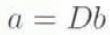
where b is a linear parameter and D, the degree-day sum above a certain temperature threshold (T u), is simply the integral under the seasonal-temperature expression (Equation (3)).
Comparison of the Model With The Present-Day Situation
The first step is to see whether the model can predict present-day distributions of precipitation, snowfall and mass balance. Only if these simulations are successful can we have the confidence to proceed to experiments during glacial conditions. An initial test of the model is to see whether it produces suitable atmospheric-moisture values. The model’s predictions of total atmospheric water-moisture consent are shown in Figure 1 and produce values of 10–15 mm in winter and 12–17 mm in summer. These values are close to general estimates (Reference Barmon and Steele.Bannon and Steele, 1960) and show the same seasonal trends.
Another significant second test of the model is its ability to simulate present-day precipitation patterns. Predicted summer, winter and annual total precipitation estimates are shown in Figure 2. Bearing in mind the paucity of precipitation data for the region, the predicted distribution of mean annual precipitation shows a good match with measured values of precipitation (Reference Miller and SchwerdtfegerMiller, 1976). In particular, the model picks up the magnitude and strong east-west gradient. There is a predicted gradient from 1000–2000 mm in the west to less than 150 mm in the east. The latitudinal precipitation gradient is also clear in the east, with drier climates in warmer latitudes. The model shows a very patchy precipitation distribution with strong local contrasts. whereas the published maps have smoothed contours. Probably, the model is realistic in that it explicitly shows changes associated with local topographic variations. The poorest match of the model is that it produces relatively low precipitation values in the coastal margin of the south-west. The modelled coastal values of 1000–2000 mm are lower than reality where values may be up to 5000 mm (Reference Miller and SchwerdtfegerMiller, 1976). Possibly, the model underestimates rain-fall due to advection. The high modelled values in the Andes agree with some recent measured values over the ice fields of 6000–700 mm (Reference Escobar, Vidal, Garin, Naruse., Naruse and AniyaEscobar and others, 1992).
Modelled precipitation (mm) for (a) summer, (b) winter, and (c) the year as a whole. The summer and winter values are given as mean annual equivalent rates fur comparison. The overall precipitation distribution compares favourably with measured distributions, showing the stong west-east precipitation graditient and absolute values close to measured values. Thick lines represent 1000 m contour intervals.

The variations in summer and winter precipitation match measured seasonal variations. In winter, both the model and measured values inidicate high precipitation throughout western Chile. In the model this is caused directly by cool land temperatures in comparison to the adjacent sea. Summer precipitation is lower overall. Precipitation to the east and in the Atlantic is less affected by seasonal changes, except in northern Argentina where precipitation increases because of the slackening of the westerlies in summer. This latter feature is also reproduced by the model.
The model calculates the proportion of precipitation that falls as snow, and this is shown in Figure 3a. As expected, snowfall is highest on the most elevated part of the Andean chain and on the higher parts of the plains in the lce of the Andes where winter temperatures are lowest. There is a latitudinal gradient in that there is more snow in the south than in the north. The highest values of snowfall are in the areas of highest precipitation. This pattern agrees with that given by Reference KadomtsevaKadomtseva (1987). Snow mass balance is shown in Figure 3b. This shows positive mass-balance values only in the vicinity of the main ice fields of today, notably Hielo Patagònico Sur, Hielo Patagònico Norte and Hielo Cordillera Darwin. In this case seasonal snow is melted is from all but the highest, wettest elevations. The good fit with the distribution of existing ice caps is encouraging and offers some degree of confidence in the model.
(a) Predicted present-day snowfall (mm a−1 w.e.) and (b) present-day mass balance over a year (mm a−1 w.e.). There is a good fit between the areas predicted to have a positive mass balance and the location of present ice fields.

Modelling Glacial Conditions
We run the model under glacial conditions for two main reasons. First, it provides a means of appraising the model under extreme conditions and discerning whether or not it may be applied successfully to former ice caps. Secondly, the model can be used to assess the relative importance to ice-cap mass balance of external forcing factors, such as temperature and pressure fields, and internal factors such as ice-cap topography.
In order to simulate maximum glacial conditions we set temperatures throughout the region at 4° C lower than present and shifted the pressure distribution north by 3° latitude. The temperature shift is an arbitrary figure which is a little lower than the 3° C indicated by our own modelling of the ice cap during the Last Glacial Maximum (Hulton and others, 1994), less than the ~6° C estimated for the same time from palaeoecological evidence (Reference HeusserHeusser, 1989a) and former moraines (Reference Porter.Porter, 1981), and in the middle of the global estimates of cooling during the Last Glacial Maximum (Reference Broecker and Denton.Broecker and Denton, 1990; Reference BarronBarron, 1992). The northward shift of the pressure fields is implicit in our previous modelling (Hulton and others, 1994) and the work of Reference HeusserHeusser (1983, Reference Heusser1989b,Reference Heusserc) The wholesale shifting of the pressure system tends to increase wind speeds in all but the most southerly locations. We ran the model under a full-glacial climate with ice-cap topography and also without an ice cap in order to test the model’s sensitivity to topography.
Running the model with an ice cap results in an entirely different precipitation pattern (Fig. 4a) from that of the present day (Fig. 2). Precipitation is concentrated along the western front of the ice cap. and the leeward precipitation gradient steepens. The already strong west-east precipitation contrast strengthens. Naturally, the snowfall pattern (Fig. 4b) follows the precipitation distribution strongly, but altitudes are high enough to allow snowfall over all of the ice cap. The mass-balance distribution (Fig. 4c) closely mirrors the location of the ice cap with mass-balance rates between 0.0 and 0-5 m a−1 over most of the ice-cap surface, but rising to over 4 m a−1 in the southwest.
Full-glacial conditions applied to the maximum Patagonian ice cap as modelled by Hulton and others (1941). For the run, temperatures are lowered by 4° C and pressure fields moved north by 3° lat., compared to the present day. Above, predictions of (a) precipitation, (b) snowfall, and (c) mass balance on and around the ice cap. The zone of maximum snow accumulation is on the western windward flanks of the ice cap, especially south of 43° S. Below, full-glacial climate conditions without an ice cap are also shown. Predictions of (d) precipitation, (e) snowfall, and (f) mass balance. Units are mm a−1 w.e. throughout

The full-glacial scenario produces an energetic western ice cap constrained by ocean caking and an eastern ice cap limited by moisture supply. The system experiences positive feed-back in that, as the ice cap evolves, it interrupts the westerly flow of moisture-laden air increasingly effectively. The increase in precipitation gives rise to an additional lall in ELA over and above that which might be related to a reduction in temperatures. But the very presence of the ice cap also limits precipitation which hinders its eastward expansion. In such a system, the zone of high snow accumulation migrates upwind and the effect intensifies as the ice sheet evolves. In effect, it accelerates its own growth towards the windward flank and becomes self-limiting on the lee side.
Perspective on the magnitude of this effect is provided by running the full-glacial climate without an ice cap. In such a case, precipitation is similar to that of the present day, but snowfall and mass balance are much higher. Comparison of the two sets of predictions shows that the existence of the ice cap has three main effects: it shifts the centre of maximum mass balance westwards by 80 km; it increases the area of maximum mass balance by an order of magnitude; and it increases the aridity of the lee flank where total precipitation in the adjacent plains is reduced by 250mm (50%). The effect is especially strong in the north and south where the topographic contrasts between glacial and non-glacial episodes are strongest.
These experiments shed light on the respective parts played by the different factors affecting precipitation and mass balance during a glacial cycle. The main conclusion is that, in a maritime climate with high rates of precipitation, a lowering of temperatine is much more important in initiating glaciation than a change in wind fields. Once glaciation is initiated, however, the latter effect influnces glacier growth. Particularly striking is the significant role of ice-surface topography in changing the pattern of precipitation both on the ice cap itself and for a considerable distance in the lee. The implications are that the response of the Patagonian ice cap to Forcing is non-linear and that a relatively small degree of initial forcing is sufficient to trigger a phase of rapid growth. The reason for this sensitivity relates to the presence of the Andes lying athwart the westerlies and close to the glaciation limit today. This sensitivity of the Patagonian ice cap to change agrees with our earlier work using a less sophisticated representation of mass balance.
Conclusions
This investigation of the links between precipitation, snow mass balance and ice-cap behaviour yields three main conclusions.
-
1. A vertically integrated moisture-balance equation is able to reproduce successfully the present-day distribution of precipitation, snowfall and snow mass balance in Patagonia and can be applied to former ice caps.
-
2. The model provides a means of distinguishing the effects on ice-cap growth of external forcing factors, such as wind fields and temperature, and internal factors such as changing ice-surface topography. The effect of topographic feed-back on mass balance is as important in ice-cap growth as the initial temperature-change mass-balance/altitude feed-back. Moreover, the effect is highly variable from place to place. This suggests caution when interpreting the results of models that rely on spatially and temporally fixed mass-balance/altitude relationships (Reference Huybrechts, Letréguilly and Reeh.Huybrechts and others, 1991; Reference Fastook and Prentice.Fastook and Prentice, 1994).
-
3. The model has the advantage that it can be refined by comparison both with modern climate data and with the palaeoecological record of the past. The palaeo-predic-tions of precipitation, snowfall and mass balance can act as hypotheses in need of empirical testing.
Acknowledgements
The work which forms the basis of this paper was generously funded by a U.K. Natural Environment Research Council grant (GST/02/544) to D.E. Sugden, CM. Clapperton and R. G. Healey.



