
 E[λ2(t)]



In the course of some research on Hawkes process parameter estimation with missingness, we needed to calculate the moments of the event count over a fixed time window. We found many useful results in [Reference Cui, Hawkes and Yi1], which provides elegant and easily understood tools and a theoretical framework for deriving these moments. During our explorations of their many valuable results, we discovered a couple minor inconsistencies between formulas provided for some expected values and the simulated values of those quantities in our work. To address these issues, we carefully revisited the calculations and discovered some small omissions in two results from [Reference Cui, Hawkes and Yi1]. We corrected these errors and compiled our findings into this correction note. In the following sections, we present the corrected formulas along with step-by-step derivations and simulation results that validate these corrections.
1. Correction 1: expression of
 $\mathbb{E}[\lambda^2(t)]$

On p.114 of [Reference Cui, Hawkes and Yi1], for
 $\alpha\neq\beta$
, expression of
 $\mathbb{E}[\lambda^2(t)]$
is
 \begin{equation}\mathbb{E}[\lambda^2(t)]=\left[\frac{\Delta_{11}}{\alpha-\beta}+\nu^2-\frac{\Delta_{12}}{\alpha-\beta}\right]e^{-2(\alpha-\beta)t}\end{equation}
where
 \begin{align*}\Delta_{11}&=(\alpha^2+2\beta\nu)\nu\left[\frac{\alpha e^{3(\alpha-\beta)t}}{3(\alpha-\beta)}-\frac{\beta e^{2(\alpha-\beta)t}}{2(\alpha-\beta)}\right] \\\Delta_{12}&=(\alpha^2+2\beta\nu)\nu\left[\frac{\alpha}{3(\alpha-\beta)}-\frac{\beta}{2(\alpha-\beta)}\right]\end{align*}
The corrected formula is
 \begin{equation} \mathbb{E}[\lambda^2(t)] = \frac{\nu \left[ (\alpha^2 + 2\beta \nu)(\beta - 2\alpha e^{(\alpha - \beta)t}) + \alpha^2(2\alpha - \beta + 2\nu)e^{2(\alpha - \beta)t} \right]}{2(\alpha - \beta)^2}\end{equation}
2. Correction 2: Eq.(13)
In Eq. (13) of [Reference Cui, Hawkes and Yi1], for
 $\alpha\neq\beta$
, expression of
 $\mathbb{E}[N(t)\lambda(t)]$
is
 \begin{equation} \mathbb{E}[N(t)\lambda(t)]=e^{(\alpha-\beta)t}\int_0^t\beta\nu\mathbb{E}[N(u)] + \alpha\mathbb{E}[\lambda(u)]+\mathbb{E}[\lambda^2(u)]du\end{equation}
The corrected formula is
 \begin{equation} \mathbb{E}[N(t)\lambda(t)]=e^{(\alpha-\beta)t}\int_0^te^{-(\alpha-\beta)u}\big\{\beta\nu\mathbb{E}[N(u)] + \alpha\mathbb{E}[\lambda(u)]+\mathbb{E}[\lambda^2(u)]\big\}du\end{equation}
3. Derivation of correction 1
Solving ODE Eq. (12) in [Reference Cui, Hawkes and Yi1], with initial condition
 $\mathbb{E}[\lambda^2(0)]=\nu^2$
,
 $$\frac{d}{dt}\mathbb{E}[\lambda^2(t)]=(2\beta\nu+\alpha^2)\mathbb{E}[\lambda(t)]+(2\alpha-2\beta)\mathbb{E}[\lambda^2(t)]$$
Assume
 $\alpha\neq\beta$
, in Eq.(10) of [Reference Cui, Hawkes and Yi1] shows that
 $$\mathbb{E}[\lambda(t)]=-\frac{\beta\nu}{\alpha-\beta}+\frac{\alpha\nu}{\alpha-\beta}e^{(\alpha-\beta)t}$$
Let
 $y(t) = \mathbb{E}[\lambda^2(t)]$
. Substituting
 $\mathbb{E}[\lambda(t)]$
into the ODE, and simplify the terms:
 \[\frac{dy}{dt} = \frac{(2\beta \nu + \alpha^2)(-\beta \nu)}{\alpha - \beta} + \frac{(2\beta \nu + \alpha^2)(\alpha \nu)}{\alpha - \beta} e^{(\alpha - \beta)t} + (2\alpha - 2\beta)y(t)\]
Reorganizing the equation:
 \[\frac{d}{dt} \left( e^{-(2\alpha - 2\beta)t} y(t) \right) = \frac{(2\beta \nu + \alpha^2)(\alpha \nu)}{\alpha - \beta} e^{-(\alpha - \beta)t} + \frac{(2\beta \nu + \alpha^2)(-\beta \nu)}{\alpha - \beta} e^{-(2\alpha - 2\beta)t}\]
Let
 $C_1 = \frac{(2\beta \nu + \alpha^2)(\alpha \nu)}{\alpha - \beta}$
and
 $C_2 = \frac{(2\beta \nu + \alpha^2)(-\beta \nu)}{\alpha - \beta}$
, the general solution for y(t) is:
 \[y(t) = -\frac{C_1}{\alpha - \beta} e^{(\alpha - \beta)t} - \frac{C_2}{2\alpha - 2\beta} + C_3 e^{(2\alpha - 2\beta)t}\]
Determining the Constant
 $C_3$
by condition
 $y(0) = \nu^2$
, the final solution for
 $\mathbb{E}[\lambda^2(t)]$
is:
 \[\mathbb{E}[\lambda^2(t)] = \frac{\nu \left[ (\alpha^2 + 2\beta \nu)(\beta - 2\alpha e^{(\alpha - \beta)t}) + \alpha^2(2\alpha - \beta + 2\nu)e^{2(\alpha - \beta)t} \right]}{2(\alpha - \beta)^2}\]
3.1. Comparison of the two formulas
Formula from [Reference Cui, Hawkes and Yi1] can be reformulated as following:
 \begin{align*}\mathbb{E}[\lambda^2(t)]=&-\frac{(\alpha^2+2\beta\nu)\beta\nu}{2(\alpha-\beta)^2}+\frac{(\alpha^2+2\beta\nu)\alpha\nu}{3(\alpha-\beta)^2}e^{(\alpha-\beta)t} \\&+\left[\nu^2-\frac{(\alpha^2+2\beta\nu)(2\alpha-3\beta)\nu}{6(\alpha-\beta)^2}\right]e^{-2(\alpha-\beta)t}\end{align*}
The corrected formula:
 \begin{align*}\mathbb{E}[\lambda^2(t)] &= \frac{\nu \left[ (\alpha^2 + 2\beta \nu)(\beta - 2\alpha e^{(\alpha - \beta)t}) + \alpha^2(2\alpha - \beta + 2\nu)e^{2(\alpha - \beta)t} \right]}{2(\alpha - \beta)^2}\\&=\frac{(\alpha^2+2\beta\nu)\beta\nu}{2(\alpha-\beta)^2}-\frac{(\alpha^2+2\beta\nu)\alpha\nu}{(\alpha-\beta)^2}e^{(\alpha-\beta)t}+\frac{\alpha^2(2\alpha-\beta+2\nu)\nu}{2(\alpha-\beta)^2}e^{2(\alpha-\beta)t}\end{align*}
Notice that for
 $\alpha<\beta$
(stationary condition for Hawkes process with exponential kernel), the term
 $e^{-2(\alpha-\beta)t}$
in expression of [Reference Cui, Hawkes and Yi1] will dominate the expected value when t gets large.
3.2. Check the formula by Monte-Carlo simulation
Simulation setup:
-
• number of simulated datasets to get MC estimator:
$n_{\text{sim}}=1,000,000$
; -
• baseline intensity: low, medium, high
$\nu=0.5, 2.0, 5.0$
; -
• combinations of
$\alpha,\beta$
:
$(\alpha,\beta)=\{(0.5,1.0),(1.0,1.5),(1.5,2.0)\}$
; -
• simulation time horizon:
$T=10$
.


Figure 1 shows the simulation comparison results. See appendix A for simulation code, and appendix B for complete simulation tables.
Plot of the logarithm of the ratio
 $\mathbb{E}[\lambda^2(t)] / \mathbb{E}_{\text{MC}}[\lambda^2(t)]$
, where
 $\mathbb{E}_{\text{MC}}[\lambda^2(t)]$
is a Monte Carlo estimator based on 1,000,000 simulated Hawkes process realizations. The red line corresponds to the formula from [Reference Cui, Hawkes and Yi1], and the blue line represents the corrected formula. When the formula closely matches the MC estimator, the logarithmic ratio is expected to be close to 0.

Figure 1 Long description
The image contains a series of nine line graphs arranged in a 3x3 grid. Each graph plots the logarithm of the ratio of expected values for a Hawkes process, comparing a formula from a reference and a corrected formula. The x-axis represents time (t) ranging from 0 to 10, and the y-axis represents the logarithm of the ratio of the expected values. The red line corresponds to the formula from the reference, and the blue line represents the corrected formula. The graphs are organized into three columns, each with different parameter values (alpha, beta) and three rows, each with different values of nu (0.5, 2.0, 5.0). When the formula closely matches the Monte Carlo estimator, the logarithmic ratio is expected to be close to 0. The red lines show an increasing trend, while the blue lines remain constant near 0, indicating the corrected formula aligns better with the Monte Carlo estimator.
4. Derivation of correction 2
ODE Eq.(8) in [Reference Cui, Hawkes and Yi1] is
 $$\frac{d}{dt}\mathbb{E}[N(t)\lambda(t)]=\beta\nu\mathbb{E}[N(t)] + \alpha\mathbb{E}[\lambda(t)]+(\alpha-\beta)\mathbb{E}[N(t)\lambda(t)]+\mathbb{E}[\lambda^2(t)]$$
With initial condition
 $\mathbb{E}[N(0)\lambda(0)]=0$
, for
 $\alpha\neq\beta$
. denote
 $g(t) = \beta\nu\mathbb{E}[N(t)] + \alpha\mathbb{E}[\lambda(t)] +\mathbb{E}[\lambda^2(t)]$
and
 $f(t)=\mathbb{E}[N(t)\lambda(t)]$
, then
 \begin{align*}&f'(t)=(\alpha-\beta)f(t) + g(t)\\\iff&e^{-(\alpha-\beta)t}f'(t)-(\alpha-\beta)e^{-(\alpha-\beta)t}f(t)=e^{-(\alpha-\beta)t}g(t)\\\iff&f(t)=e^{(\alpha-\beta)t}\int_0^te^{-(\alpha-\beta)u}g(u)du\end{align*}
which leads to the corrected formula.
Appendix A. Simulation R code


Appendix B. Complete simulation results
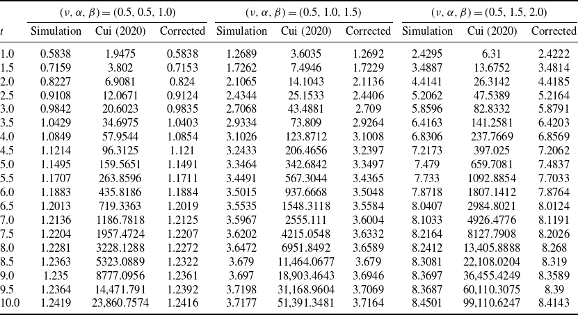
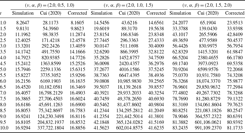
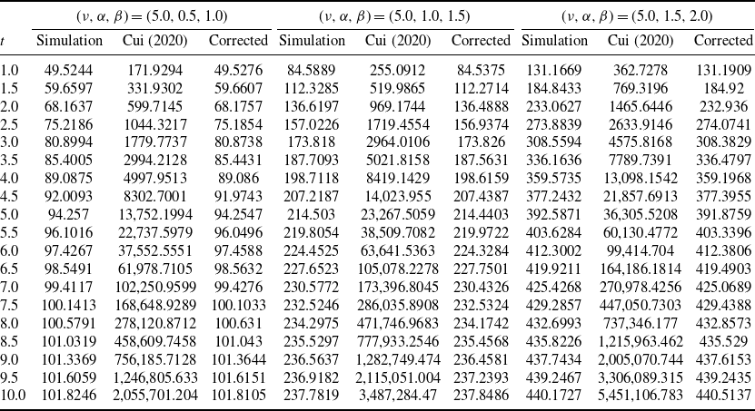
The complete simulation data for Figure 1 are listed in this section.
 $\mathbb{E}[\lambda^2(t)]$
, low baseline intensity,
 $\nu=0.5$
.

Table B1 Long description
The table presents a comparison of simulation, Cui 2020, and corrected values for different parameter sets. It includes three main sections, each with different parameter values: (0.5, 0.5, 1.0), (0.5, 1.0, 1.5), and (0.5, 1.5, 2.0). The table has 11 rows and 9 columns. The columns are labeled as t, Simulation, Cui 2020, Corrected for each parameter set. The rows are labeled with time values ranging from 1.0 to 10.0. Notable trends include increasing values across all columns as time progresses, with significant differences between the simulation, Cui 2020, and corrected values.
 $\mathbb{E}[\lambda^2(t)]$
, medium baseline intensity,
 $\nu=2.0$
.

Table B2 Long description
The table presents a comparison of simulation, Cui 2020, and corrected values for different parameters. It includes three sets of parameters: (2.0, 0.5, 1.0), (2.0, 1.0, 1.5), and (2.0, 1.5, 2.0). The table has 11 rows and 10 columns, with headers for time (t) and the three sets of parameters. Each row provides values for simulation, Cui 2020, and corrected data. Notable trends include increasing values across all columns as time progresses, with significant differences between the simulation, Cui 2020, and corrected values.
 $\mathbb{E}[\lambda^2(t)]$
, high baseline intensity,
 $\nu=5.0$
.

Table B3 Long description
The table presents simulation results for different parameter sets in a mathematical model with high baseline intensity and nu equals 5.0. It includes columns for time (t), simulation values, Cui (2020) values, and corrected values across three different parameter sets: (5.0, 0.5, 1.0), (5.0, 1.0, 1.5), and (5.0, 1.5, 2.0). The table has 11 rows and 13 columns. Notable trends include increasing values across all columns as time progresses. For example, at t equals 1.0, the simulation values start at 49.5244, 84.5889, and 131.1669 for the respective parameter sets, and these values increase significantly by t equals 10.0 to 101.8246, 3,487,284.47, and 5,451,106.783. The corrected values also show a similar increasing trend.

 E[λ2(t)]/EMC[λ2(t)]
 EMC[λ2(t)]
 E[λ2(t)]
 ν=0.5
 E[λ2(t)]
 ν=2.0
 E[λ2(t)]
 ν=5.0


