





1. Introduction
Glaciers are important water resources for downstream populations, especially in arid areas of the Himalaya–Karakoram (Armstrong and others, Reference Armstrong2019; Azam and others, Reference Azam2021), and their behavior is influenced by climatic changes. Quantifying regional and local climate-induced changes in glacier mass and extent across Himalaya–Karakoram (∼39 660 glaciers covering an area of ∼40 800 km2) is challenging due to glacier heterogeneity, rugged terrain and difficult access (Bolch and others, Reference Bolch, Wester, Mishra, Mukherji and Shrestha2019). Only 38 glaciers (0.09% of the total number in Himalaya–Karakoram) are monitored in the field using the traditional glaciological method (Azam, Reference Azam2026), limiting the understanding of the response of glaciers to climatic variability in these areas. Equilibrium line altitudes (ELAs) are used as indicators of glacier mass balance and their fluctuations with respect to climate. The ELA of a glacier refers to the spatially averaged altitude of all points on the surface of the glacier where the mass balance is zero at a given point in time (Braithwaite and Raper, Reference Braithwaite and Raper2009; Cuffey and Paterson, Reference Cuffey and Paterson2010), and it varies from year to year with respect to climate variables (temperature and precipitation). Continuous systematic monitoring of glacier ELAs is important for the calibration/validation of glacio-hydrological models (Azam and others, Reference Azam2021; Srivastava and Azam, Reference Srivastava and Azam2022) and for the reconstruction of glacier mass balance (Davaze and others, Reference Davaze, Rabatel, Dufour, Hugonnet and Arnaud2020; Chandrasekharan and Ramsankaran, Reference Chandrasekharan and Ramsankaran2023), but this poses a number of challenges. ELAs are best determined in the field from point ablation and accumulation measurements as the altitude where the mass balance equals zero (Cuffey and Paterson, Reference Cuffey and Paterson2010). The ELA derivation is sensitive to the accuracy of the digital elevation model (DEM) and glacier outlines used to extract the altitude, that is, many studies rely on fixed outlines and DEMs that do not accurately reflect changes in glacier elevation, thus introducing uncertainties (Braithwaite and Raper, Reference Braithwaite and Raper2009; Oien and others, Reference Oien, Rea and Bingham2022).
In remote, inaccessible high-altitude areas such as the Himalaya–Karakoram, consistent, systematic field-based ELA measurements are limited to a few glaciers (Dobhal and others, Reference Dobhal, Mehta and Srivastava2013; Sherpa and others, Reference Sherpa2017; Wagnon and others, Reference Wagnon2021; Azam and others, Reference Azam2024, Reference Azam2025). Therefore, multitemporal satellite-derived snowline altitudes (SLAs) are used to estimate the season maximum SLA at the end of the ablation season (denoted here and thereafter as ‘SLAmax’), and these are used as a proxy for the glacier ELA. However, the commonly held assumption that SLAmax approximates the true ELA has not been thoroughly tested across the Himalaya–Karakoram region. Furthermore, numerous studies commonly derived snowline positions from a single or a limited number of images at the end of the ablation season (Bajracharya and others, Reference Bajracharya, Maharjan and Shrestha2014; Thakuri and others, Reference Thakuri2014). Similar approaches were applied to relate remotely sensed ELAs to glacier mass-balance variability and retreat patterns (Mir and others, Reference Mir, Jain, Saraf and Goswami2014; Rashid and others, Reference Rashid, Majeed, Aneaus and Pelto2020). At the regional scale, SLAs at the end of the ablation season were analyzed using MODIS time series for High Mountain Asia (Tang and others, Reference Tang, Wang, Deng, Wang, Jiang and Sang2020). Moreover, Landsat imagery for nine glaciers located in western, central and eastern Himalaya was used to interpret the highest seasonal SLA as indicative of the ELA (Wang and others, Reference Wang, Tang, Deng, Hu, You and Zhao2023). None of these studies explicitly evaluates the assumption that SLAmax ≈ ELA against field-based ELAs. In contrast, analyses based on dense temporal sampling reveal pronounced seasonal and intraseasonal SLA variability, indicating that ELA estimates derived from a single image may be sensitive to the time of acquisition (Spiess and others, Reference Spiess, Huintjes and Schneider2016; Loibl and others, Reference Loibl, Richter and Grünberg2025; Sasaki and others, Reference Sasaki, Miles, Pellicciotti, Sakai and Fujita2025).
Remote-sensing techniques can help fill this gap, given the large amount of satellite data and the evolving automation of the SLA extraction and post-processing routines. In the last two decades, optical remote sensing has been used to extract glacier SLAs (Pelto, Reference Pelto2011; Huss and others, Reference Huss2013; Mernild and others, Reference Mernild, Lipscomb, Bahr, Radić and Zemp2013; Tawde and others, Reference Tawde, Kulkarni and Bala2016; Rabatel and others, Reference Rabatel2017; Yue and others, Reference Yue, Li, Zhao, Li, Wang and Wang2021). These studies further demonstrated the importance of seasonal and sub-seasonal SLA time series for understanding glacier mass-balance variability and snowline fluctuations. SLA extraction techniques evolved from manual methods (Rabatel and others, Reference Rabatel, Dedieu and Vincent2016; Barandun and others, Reference Barandun2018; Chandrasekharan and others, Reference Chandrasekharan, Ramsankaran, Pandit and Rabatel2018) to semiautomated approaches based on various band ratios and indices from Sentinel-2, Landsat, ASTER, MODIS or SPOT images combined with DEMs. Band ratio images were generally thresholded using a fixed value (Rastner and others, Reference Rastner, Nicholson, Sailer, Notarnicola and Prinz2015; Racoviteanu and others, Reference Racoviteanu, Rittger and Armstrong2019) or variable values based on Otsu thresholding of the near-infrared band (Rastner and others, Reference Rastner2019; Liu and others, Reference Liu, Li, Zhang, Tian, Zhou and Chen2021). Other studies used multi-step classification schemes based on surface albedo (Lei and others, Reference Lei, Zeng and Zhang2012; Naegeli and others, Reference Naegeli, Huss and Hoelzle2019; Barandun and others, Reference Barandun2021). Recent attempts to further automate these approaches include the use of Google Earth Engine (Liu and others, Reference Liu, Li, Zhang, Tian, Zhou and Chen2021; Loibl and others, Reference Loibl, Richter and Grünberg2025; Lorenz and others, Reference Lorenz2025) or machine learning algorithms (Li and others, Reference Li, Huang, Chen and Tian2012; Prieur and others, Reference Prieur, Rabatel, Thomas, Farup and Chanussot2022). Despite these advances, continuous sub-monthly SLA estimates suffer from limitations in high mountain environments due to the presence of deep/cast shadow, steep slopes, snow patches, crevasses and cloud cover common in monsoon-dominated areas (Racoviteanu and others, Reference Racoviteanu, Rittger and Armstrong2019; Rastner and others, Reference Rastner2019). Attempts to overcome these challenges include the use of filters based on the percent cloud cover, standard deviation (SD) of SLA (Loibl and others, Reference Loibl, Richter and Grünberg2025), slope and elevation (Girona-Mata and others, Reference Girona-Mata, Miles, Ragettli and Pellicciotti2019; Racoviteanu and others, Reference Racoviteanu, Rittger and Armstrong2019) or percent snow cover area by elevation zone (Rastner and others, Reference Rastner2019; Prieur and others, Reference Prieur, Rabatel, Thomas, Farup and Chanussot2022; Loibl and others, Reference Loibl, Richter and Grünberg2025). Other studies restricted the SLA extraction to the center flowline of the glacier to minimize topographic effects (Rabatel and others, Reference Rabatel2017; Davaze and others, Reference Davaze, Rabatel, Dufour, Hugonnet and Arnaud2020). As a result of these challenges, SLA extraction using optical remote sensing is still laborious and has been applied to only a limited number of glaciers in the Himalaya–Karakoram region (Rabatel and others, Reference Rabatel2012; Racoviteanu and others, Reference Racoviteanu, Rittger and Armstrong2019; Chandrasekharan and Ramsankaran, Reference Chandrasekharan and Ramsankaran2023).
Previous studies established the potential of satellite-derived SLAs as proxies for ELAs for mid-latitude glaciers, where processes such as sublimation, snowdrift and wind-driven ablation typically have a limited influence on the overall seasonal to annual glacier mass balance. While these processes can have substantial localized effects, particularly in wind-exposed or high-altitude zones, their net contribution is usually minor when averaged across entire glacier surfaces (Lliboutry, Reference Lliboutry1965; Melo and others, Reference Melo, Sigmund and Lehning2024; Voordendag and others, Reference Voordendag, Goger, Prinz, Sauter, Mölg, Saigger and Kaser2024). However, in monsoon-dominated areas or the outer tropics, these surface processes can be much more significant in controlling glacier mass balance, as snowfall may occur throughout the year (Rabatel and others, Reference Rabatel2012; Wagnon and others, Reference Wagnon2013). During the monsoon, precipitation occurring as snowfall at high altitudes leads to snow accumulation, and this occurs simultaneously with ablation from ice melting and sublimation. These concurrent processes create a dynamic snowline that can fluctuate up and down throughout the season, making it challenging to determine the SLAmax that accurately represents the ELA. Additionally, wind-driven snow redistribution, rain-on-snow events and temporary seasonal snow cover in glacier ablation zones further challenge the distinction between snow and ice, complicating the interpretation of remotely sensed SLAmax as proxies for ELAs. Therefore, previous studies (e.g. Rabatel and others, Reference Rabatel2012) emphasized the importance of validating SLA-derived ELA estimates using benchmark glaciers with field data before applying this proxy to other glaciers, especially in monsoon-dominated regions or the outer tropics (Dyurgerov, Reference Dyurgerov2010; Rabatel and others, Reference Rabatel2012; Yuwei and others, Reference Yuwei, Jianqiao, Zhongming and Anan2014; Rabatel and others, Reference Rabatel, Dedieu and Vincent2016; Tawde and others, Reference Tawde, Kulkarni and Bala2016). In particular, Dyurgerov (Reference Dyurgerov2010) showed that the relationship between accumulation–area ratio (AAR) and ELA can vary, and for glaciers experiencing significant summer snowfall, it may be nonlinear or even absent.
In this study, we focus on the Khumbu region in the monsoon-dominated central Himalaya using Mera Glacier as a case study to test this assumption. Our analysis is limited to optical data without extending to multisource data fusion, as the proposed approach builds on an existing optical remote-sensing method for SLA estimation, which is still widely used. Specific goals are (1) to construct an SLA dataset at basin scale from Landsat 8/Sentinel-2 images over the period 2015–23 using a semiautomated method implemented in Python, validated with high-resolution Planet/VENμS images (3–5 m); (2) to explore sub-monthly spatiotemporal SLA fluctuations at basin/glacier scale; and (3) to test the assumption that SLAmax ≈ ELA at glacier scale by comparing the estimated remote-sensing SLAs with the field-based ELAs on Mera Glacier.
2. Methods
2.1. Study area
Our study area is the glacierized Dudh Koshi basin (∼3711 km2, 449–8761 m a.s.l.), located in the monsoon-dominated central Himalaya (Fig. 1) (Thayyen and Gergan, Reference Thayyen and Gergan2010). In this area, the Indian summer monsoon causes maximum precipitation (∼80% of the annual precipitation) during the summer months (June–September). Glaciers in these areas are referred to as ‘summer accumulation type glaciers’ (Bookhagen and Burbank, Reference Bookhagen and Burbank2006; Thayyen and Gergan, Reference Thayyen and Gergan2010). The simultaneous accumulation and ablation patterns often lead to indistinguishable glacier SLAs due to cloud and/or temporary snow cover (Brun and others, Reference Brun2015). During the summer, snowfall is frequent at higher elevations, while lower elevations may experience rainfall (Khadka and others, Reference Khadka, Brun, Wagnon, Shrestha and Sherpa2024). The post-monsoon period (October–November) marks a rapid shift to predominantly dry, sunny and cooler weather, occasionally disrupted by typhoons that can bring heavy snowfall above 4000 m a.s.l. (Shea and others, Reference Shea, Immerzeel, Wagnon, Vincent and Bajracharya2015). The winter season (December–February) is characterized by even harsher conditions, with consistently cold, arid and windy weather and minimal snowfall. During the pre-monsoon period (March–May), the weather gradually becomes warmer and wetter, making this the second wettest season of the year (Khadka and others, Reference Khadka, Wagnon, Brun, Shrestha, Lejeune and Arnaud2022). Throughout the post-monsoon, any deposited snow is often blown away by strong winds above 5000 m a.s.l. (Wagnon and others, Reference Wagnon2013).
Study area: (a) Dudh Koshi basin in the central Himalaya; (b) upper part of Dudh Koshi shown on a false-color composite of the Sentinel-2 image from 14 Jan 2016 (bands 11, 8, 4) with glaciers from the GAMDAM inventory in cyan, the subset used for validation around the Hinku subbasin in the yellow box (n = 177 glaciers) and Mera Glacier is marked with a red star; (c) Mera Glacier (cyan) shown on a Planet RapidEye image from 10 Jan 2016 (bands 5, 4, 3) with ablation stake locations marked as red dots.

1 Long description
The image A shows a map of the Himalayas with regions labeled as Karakoram, Western Himalaya, Central Himalaya and Eastern Himalaya. A scale bar indicates distances from 325 to 1,300 kilometers. The image B displays a false color composite map of the upper part of the Dudh Koshi basin with glacier outlines in cyan and a yellow box highlighting a subset area. Coordinates are marked along the edges. The image C shows a detailed view of the Mera Glacier area with ablation stake locations marked as red dots. A scale bar indicates distances from 0.5 to 2 kilometers. A legend identifies the Dudh Koshi basin, glacier outlines and Mera Glacier with respective symbols.
To test the assumption that SLAmax ≈ ELA, we focus on Mera Glacier, a small clean glacier (∼4.8 km2 in 2018, 4940–6420 m a.s.l.) located in the central part of the Dudh Koshi basin within the Hinku Valley (Fig. 1). Mera Glacier has been monitored in the field since 2007 within the framework of the GLACIOCLIM network (Wagnon and others, Reference Wagnon2013, Reference Wagnon2021). It is north-oriented, and it divides into two branches at ∼5800 m, referred to as Mera and Naulek (Wagnon and others, Reference Wagnon2013). In this study, we are only investigating the Mera branch, which has a denser network of ablation stakes, offering a priori field knowledge and opportunities for comparing the remote-sensing SLAs with the field-based ELAs. The average field-based ELA of Mera Glacier was 5618 m a.s.l. with an average AAR of 0.47 and an average annual glacier-wide mass balance of −0.41 m w.e. over the period 2007–19 (Wagnon and others, Reference Wagnon2021).
2.2. Datasets
2.2.1. Remote-sensing data
To extract glacier SLAs, we used sub-monthly, multitemporal data from Sentinel-2 and Landsat 8 sensors for the period 2015–23 (dates of the images given in Supplementary Table S1). We focused on the period 2015–23 due to the scarcity of snow and cloud-free Landsat imagery before this period. For Sentinel-2, we obtained collection 1 MSI Level-1C (L1C) data from Copernicus Open Access Hub, consisting of orthorectified top-of-atmosphere (TOA) reflectance in cartographic geometry for 13 spectral bands, with 10 m spatial resolution in the visible (VIS) and 20 m in the shortwave infrared (SWIR) bands. Two Sentinel-2 tiles cover the Dudh Koshi basin, and these were mosaicked for analysis for each date. For Landsat 8, we obtained collection 2, Level-1 data from the United States Geological Survey (USGS, 2019), which consists of radiometrically calibrated and terrain-corrected (L1TP) data provided as scaled digital numbers for 11 bands, with 30 m pixel size in VIS to SWIR bands. Since Landsat 8 has only a 16 day revisit time, there were fewer available dates compared to Sentinel-2 (5 day revisit time). For both sensors, suitable cloud-free, well-contrasted images were selected from April to December/January each year. Generally, there were fewer images from April, May, September and October due to seasonal snow and/or clouds; the most suitable images were from the dry season, November–December and even January (Supplementary Table S1). We performed atmospheric and topographic corrections on all images using the open-access Atmospheric and Radiometric Correction of Satellite Imagery (ARCSI) software (Bunting and Clewley, Reference Bunting and Clewley2018), based on the 6S radiative transfer model (Vermote and others, Reference Vermote, Tanré, Deuze, Herman and Morcette1997) (Fig. 2a). This yielded the standardized surface reflectance for all the scenes, with deep shadows masked out as NoData. For the topographic correction step in ARCSI, we used the ALOS Global Digital Surface Model (AW3D30 version 2.2, at 30 m) (Takaku and Tadono, Reference Takaku and Tadono2017), constructed from data acquired from 2006 to 2011. The reported vertical accuracy is ∼10 m in eastern Nepal, where our study area is located (Tadono and others, Reference Tadono, Ishida, Oda, Naito, Minakawa and Iwamoto2014). This DEM version contains fewer data voids and provides better shadow rendering in ARCSI in our study area, as reported by Racoviteanu and others (Reference Racoviteanu, Nicholson and Glasser2021). The AW3D30 DEM was also used in this study to extract the SLAs, as described in Section 2.3.
SLA extraction workflow showing all the inputs, outputs and their thresholds: (a) raw SLA extraction using Otsu thresholding and buffer intersection, (b) automated filtering to get the final SLAs; (c) box-and-whisker plot, where Q1, Q3, whislo and whishi represent the first and third quartiles, lowest whisker and highest whisker values, respectively.

Figure 2 Long description
The image consists of three parts labeled a, b and c. Part a shows a flowchart for raw SLA extraction using Landsat 8 and Sentinel 2 Level 1 products. It starts with standardized reflectance data processed through ARCSI, followed by NIR/SWIR greater than 1.5, separating snow and ice from other elements. Otsu thresholding is applied to NIR for snow and ice, leading to the intersection of buffers and extraction of SLA elevation values using ALOS DEM. Part b involves clipping with glacier boundaries using a 100-meter buffer, filtering using a box plot where whislo is less than elevation value less than Q3 and applying a sieve filter to remove isolated pixels, resulting in snowline altitude. Part c is a box-and-whisker plot showing SLA elevation in meters above sea level, with labeled elements including outliers, whislo, Q1, median, Q3 and whishi.
High-resolution Planet and VENμS data (3–5 m) were used to validate the Sentinel-2/Landsat 8-derived SLAs over the study period. Images from Planet RapidEye (5 m)/PlanetScope (3 m) consist of multispectral data (five and four spectral bands, respectively, in the VIS/NIR) with a positional accuracy of <10 m (PlanetLabs, 2021). We obtained Level 3A/B data, which comprises radiometrically corrected, orthorectified surface reflectance. The Franco-Israeli VENμS mission acquired images with a 2-day revisit time, 5 m spatial resolution and 12 narrow spectral bands (VIS to NIR) over the period 2017–20 in the Khumbu area. VM1 (VENμS Mission 1) products from the first acquisition phase were freely accessed through the French CNES Theia website (https://www.theia-land.fr/en/blog/product/venus/). We obtained Level 2A atmospheric corrected surface reflectance, namely the flat reflectance output products, produced by CNES on the basis of L1C/L1A TOA reflectance (Theia-Land, 2022). Planet/VENμS images were used in two ways: (1) for the snowline validation, by selecting the images closest to the dates of the Sentinel-2/Landsat 8 images (∼1–2 days) and (2) to find the highest exposed SLA for comparison with field-based ELAs on Mera Glacier (Section 2.2.3).
2.2.2. Glacier masks
Glacier masks were needed for the subsequent SLA extraction steps, and we defined these in two ways. For the Dudh Koshi basin, we used glacier outlines from the GAMDAM glacier inventory (Sakai, Reference Sakai2019), constructed using semiautomated mapping of satellite imagery (Landsat ETM+ imagery from 1999 to 2003) and manual corrections. This inventory covers 425 km2 of the Dudh Koshi basin, with a total of 462 glaciers. While there is a mismatch of ∼10 years between the date stamp of these outlines and the period of our analysis, we only used these as a glacier mask, so this should not affect the SLA extraction routine, as most glaciers have shrunk in this area (Li and others, Reference Li, Wang and Wu2022). For the detailed validation of the SLA method in the Hinku subbasin, we updated these glacier outlines using manual delineation on Planet/VENμS satellite images from 2 December 2020, to minimize any uncertainties related to glacier area estimates.
2.2.3. Field data
Field-based ELAs, point glacier mass balance and corresponding snow depths measured on Mera Glacier were obtained from the GLACIOCLIM network (https://glacioclim.osug.fr/). Ablation stakes installed on the Mera branch have been measured each year at the end of the ablation season (generally November) using the glaciological method since 2007 (Wagnon and others, Reference Wagnon2013). Field-based ELAs are estimated from the vertical mass-balance gradient using stake measurements and elevations from the 2018 Pleiades DEM as reported in Wagnon and others (Reference Wagnon2013, Reference Wagnon2021).
2.3. Snowline extraction
To extract snowlines, we built on the band-ratio method proposed by Racoviteanu and others (Reference Racoviteanu, Rittger and Armstrong2019), which was further improved here to automate and refine the SLA extraction. Specifically, we masked out the shadow areas and used the Otsu method (Otsu, Reference Otsu1975) to automatically select the appropriate threshold for every satellite image rather than using visual inspection and prior knowledge as in the study by Racoviteanu and others (Reference Racoviteanu, Rittger and Armstrong2019).
Our refined method consists of several steps implemented as conditional statements in Python (Fig. 2) and applied over the entire Dudh Koshi basin (462 glaciers). The first part (Fig. 2a) consists of separating snow and ice from the surrounding terrain using a fixed threshold based on literature, applied to a band ratio (NIR/SWIR >1.5, Sentinel-2: band 8/11, Landsat 8: band 5/6) (Racoviteanu and others, Reference Racoviteanu, Paul, Raup, Khalsa and Armstrong2009, Reference Racoviteanu, Rittger and Armstrong2019), followed by NIR band thresholding automated using the Otsu method to separate snow from ice (Racoviteanu and others, Reference Racoviteanu, Rittger and Armstrong2019). Snow and ice areas were then buffered and intersected to extract ‘raw’ snowlines as detailed in Racoviteanu and others (Reference Racoviteanu, Rittger and Armstrong2019) (Fig. 2a). In the second part, we filtered the raw SLAs to limit known outliers commonly found in both the ablation and accumulation areas of glaciers in previous studies (Racoviteanu and others, Reference Racoviteanu, Rittger and Armstrong2019) (Fig. 2b). This consisted of (a) applying a negative buffer of 100 m to the GAMDAM glacier outlines (Fig. 2b); (b) applying a threshold between Q3 (third quartile) and Whislo (lower whisker) on a box plot, chosen using a trial-and-error basis (Fig. 2b, c); and (c) applying a sieve filter on the binary image (SLA/non-SLA pixels) to further minimize common outliers in the accumulation/ablation areas (e.g. the inclusion of false positives in the accumulation area). For the sieve filtering step, we defined different thresholds for each sensor (Sentinel-2: 50 pixels and Landsat 8: 30 pixels); these thresholds were determined by several tests on glaciers of varying sizes (∼2 to ∼127 km2) to make sure we captured isolated pixel groups of various sizes; (d) SLA extraction with the output binary image and DEM to yield the ‘final’ SLAs at basin scale (Fig. 2b). Glacier SLAs were calculated as the mean elevation of all the pixels along the final snowlines within the glacier boundary. Subbasin-wide average SLAs and basin-wide average SLAs were calculated as an average of all glacier SLAs within the Hinku subbasin and Dudh Koshi basin, respectively.
2.4. Validation
We validated the remote-sensing Sentinel-2 and Landsat 8 SLAs in a subset of the Dudh Koshi basin—the Hinku subbasin (177 glaciers)—by comparing them with SLAs delineated manually on Planet/VENμS color composites (Planet: bands 4, 3, 2 and VENμS: bands 11, 7, 4). This was conducted as a double-blind experiment by a different analyst, independently of the semiautomated workflow described above. Both the semiautomated and the manually delineated SLAs were extracted from the AW3D30 DEM using the 2020 Planet/VENμS glacier mask described in Section 2.2.2. We calculated the mean SLAs from both datasets on a glacier-by-glacier basis and compared their means from 13 common dates (±1–2 days) over the period 2015–23. We calculated the accuracy of the semiautomated SLAs with respect to the Planet/VENμS SLAs as vertical root-mean-square error (RMSEz) and coefficient of determination (R 2). We also performed two-sample t tests to evaluate the differences in means between the two samples (Sentinel-2/Landsat 8 vs Planet/VENμS) and visually investigated outliers.
2.5. Comparison of remote-sensing SLAmax with the field-based ELA
To evaluate the reliability of remote-sensing SLAmax as a proxy for the ELA, we first masked out the SLAs from the basin-scale final SLAs for all the available cloud-free satellite images over this period using the Mera Glacier extent. We compared SLAmax extracted from Sentinel-2 and Landsat 8 images with field-based ELAs closest in time. Field measurements on Mera Glacier were generally performed during November, at the end of the hydrological year, and we selected our satellite data to match these dates ±1 day. This comparison was performed for each hydrological year over the period 2015–23.
2.6. Uncertainty analysis
Uncertainty in SLAs was calculated using three independent components: (1) the standard error of the mean (µ Mean); (2) vertical error of the DEM (µ DEM) and (3) uncertainty in the glacier outlines based on image spatial resolution (µ Outline). The total uncertainty was estimated as the RMSE, as in prior studies (Racoviteanu and others, Reference Racoviteanu, Rittger and Armstrong2019; Li and others, Reference Li, Wang and Wu2022; Loibl and others, Reference Loibl, Richter and Grünberg2025):
 \begin{equation}\mu_{\mathrm{Total}}=\sqrt{\mu_{\mathrm{Mean}}^2+\mu_{\mathrm{DEM}}^2+\mu_{\mathrm{Outline}}^2}\end{equation}
Here, µ Mean = σ/√N, where σ and N are the SD and number of elevation values used per SLA estimate, respectively. µ DEM = ±10 m, that is, vertical accuracy of AW3D30 in eastern Nepal, where our study area is located (Tadono and others, Reference Tadono, Ishida, Oda, Naito, Minakawa and Iwamoto2014). µ Outline is considered to be half of the pixel size of the Landsat 8 and Sentinel-2 image (i.e. ±15 and ±5 m, respectively).
3. Results
3.1. Performance and validation of the snowline method
Over the upper Dudh Koshi basin, we processed 82 Sentinel-2 images for the period 2016–23 and 19 Landsat 8 images for the period 2015–22 (Supplementary Table S1). We detected a total of 6330 glacier SLAs ranging from 4578 ± 33 to 5900 ± 23 m for the Dudh Koshi basin. We masked them with the Hinku subbasin outlines and obtained 3176 glacier SLAs. Initially, the raw SLAs exhibited outliers near the glacier ridgelines, crevasses, shadows and snow patches in the ablation area, etc. The filtering step (Fig. 2b) allowed the removal of these outliers, an example shown with Sentinel-2 and Landsat 8 images acquired 4 days apart (Fig. 3). The outliers, initially present around the glacier ridgelines (white arrows in Fig. 3a and c), were removed by the negative buffer applied to glacier boundaries. Similarly, the outliers with extreme elevation values in the accumulation areas, which fell outside the 100 m buffer from the ridgeline, were removed using the box plot filtering (green arrow in Fig. 3c). The remaining isolated outliers were removed by sieve filtering (yellow arrow in Fig. 3a). Most of the outliers/erroneous pixels were successfully removed, resulting in more reliable and clearer SLAs (Fig. 3b and d).
Illustration of the SLA filtering step showing raw SLAs (panels a, c) and the final SLAs (panels b, d) on two randomly selected glaciers in the Hinku subbasin for Sentinel-2 (top row, 20 Oct 2018, bands 11, 8, 4) and Landsat 8 (bottom row, 24 Oct 2018, bands 6, 5, 4). Arrows point to outliers near glacier ridgeline (white) at high elevations (green) and isolated pixels (yellow).

Figure 3 Long description
The image consists of four panels labeled a, b, c and d. Panel a shows a glacier with marked outliers indicated by arrows and a red snowline. Panel b displays the same glacier without the outliers, maintaining the snowline. Panel c illustrates another glacier with outliers marked by arrows and a red snowline. Panel d shows the same glacier as panel c, but without the outliers, retaining the snowline. The glacier boundaries are outlined in each panel.
For the Hinku subbasin, final sub-monthly subbasin-wide average SLAs for the period 2015–23 are shown in Table 1. Subbasin-wide average SLA was lowest in 2016 (5484 ± 39 m) and highest in 2018 (5645 ± 34 m) (Table 1), with a mean of 5575 ± 30 m over the period 2015–23. Since the extent of the Planet scenes varied annually depending on acquisitions, only 381 glacier SLAs out of the total 6330 glacier SLAs extracted from Sentinel-2/Landsat 8 at basin scale could be compared with the manually delineated Planet/VENμS SLAs in the Hinku subbasin (Table 1). The correlation improved from R 2 = 0.41 (RMSEz = 188.8 m) for the raw SLAs (nonfiltered) to R 2 = 0.80 (RMSEz = 61.3 m) when using the filtered SLAs (Fig. 4). Yearly comparisons between Sentinel-2/Landsat 8 and Planet/VENμS SLAs yield R 2 ranging from 0.65 in 2016 to 0.90 in 2020 (Supplementary Fig. S1). Despite the variability in R 2 which may be due to surface conditions, as discussed in Section 4.2, the means of the two sets of samples (Sentinel-2/Landsat 8 final SLAs vs Planet/VENμS) differed by only a few meters (Table 1); the differences were not statistically significant at the 95% confidence level based on the two-sample t test assuming unequal variances (p > 0.05, df = 791, where df denotes the degree of freedom).
Regression between the semiautomated Sentinel-2/Landsat 8 glacier SLAs and the manually delineated Planet/VENμS glacier SLAs (a) before and (b) after automated filtering over the period 2015–23.

Figure 4 Long description
The image contains two scatter plots. The first plot, labeled 'a', shows raw glacier SLAs (non-filtered) with semi-automated glacier SLA on the y-axis and manually-delineated glacier SLA on the x-axis, both in meters above sea level. The equation is Y equals 0.74 times X plus 1557.5, with R squared equals 0.41 and RMSE equals 188.8 meters. The second plot, labeled 'b', shows final glacier SLAs (filtered) with the same axes. The equation is Y equals 0.83 times X plus 961.1, with R squared equals 0.80 and RMSE equals 61.3 meters. Both plots display data points and trend lines, indicating improved correlation in the filtered data.
Summary statistics for Sentinel-2/Landsat 8 (S2/L8) subbasin-wide average SLAs over the Hinku subbasin (177 glaciers) and validation with manually delineated subbasin-wide average SLAs from Planet/VENμS images (denoted here as PS/VE) ±1–2 days over the period 2015–23.

Table 1 Long description
The table presents a comparison of glacier surface level averages between Sentinel-2/Landsat-8 and Planet/VENμS images over the Hinku sub-basin from 2015 to 2023. It includes data on the number of surface level averages, their measurements, mean differences, root mean square errors, and correlation coefficients. Key data points show mean differences ranging from 1 to 40 meters, with correlation coefficients mostly above 0.7, indicating strong agreement between the two measurement methods. Notable trends include consistently high correlation coefficients, suggesting reliable validation of Sentinel-2/Landsat-8 data by Planet/VENμS images. The root mean square error values vary, reflecting differences in measurement precision across dates. Overall, the data suggests a robust validation process, though variations in mean differences highlight potential measurement discrepancies.
The residuals plotted against the averages of manually delineated SLAs and semiautomated final SLAs (Fig. 5a) follow a normal distribution, with a mean residual of 4.25 m (Fig. 5a). The majority of the residuals (93%) fall within the limits of agreement (±1.96 SD) (Bland and Altman, Reference Bland and Altman1986), marked as shaded area in Fig. 5, with only 27 residuals falling outside the limits of agreement. Some of the outliers in Fig. 5a are most likely due to the presence of snow patches in the ablation areas, as shown in Fig. 6a. In other situations, parts of the glacier surface near the shadow have a lower reflectance and get misclassified as ice, resulting in false SLAs near the shadow edge, higher than the actual SLA location (i.e. negative residuals) (Fig. 6a). Supraglacial lakes were misclassified as snow due to the high reflectance of frozen lakes in winter (Fig. 6b), resulting in false snowlines at lower altitudes than the actual snowline, which appeared as positive residuals in Fig. 5a. Low reflectance crevassed areas shown in Fig. 6c and spectrally mixed pixels (snow/ice/shadow) (Fig. 6d) impact the reflectance histogram utilized for Otsu thresholding, resulting in multiple peaks of different reflectance, and a threshold that is either lower or higher than the optimal threshold needed to effectively separate snow and ice. These resulted in positive and negative residuals, respectively (Fig. 5a).
(a) Bland–Altman plot of the average SLAs and the residuals (manually delineated SLA minus semiautomated SLA); (b) normal distribution curve of residuals. The upper and lower limits of agreement correspond to ±1.96 times the SD from the mean residual.

Figure 5 Long description
The image contains two plots. The first plot, labeled 'a', is a Bland-Altman plot showing residuals in meters on the y-axis against the average SLA in meters above sea level on the x-axis, ranging from 5200 to 6000. Data points are scattered within a shaded area, indicating limits of agreement. The second plot, labeled 'b', is a normal distribution curve of residuals with probability density function values on the x-axis and residuals in meters on the y-axis, ranging from negative 200 to 200.
Examples of challenging situations where the semiautomated method failed to accurately detect the SLA: (a) glaciers with snow patches in the ablation area, (b) shadows and supraglacial lakes, (c) crevasses and (d) mixed pixels (snow/ice/shadow). The background images are Sentinel-2 false-color composites (bands 11, 8, 4).

Figure 6 Long description
The image contains four satellite images labeled a, b, c and d, each showing snowlines. Image a, dated December 2016, displays semi-automated snowlines in yellow and manually-delineated snowlines in red. Image b, from December 2020, also shows both types of snowlines. Image c, another from December 2016, features the same snowline delineations. Image d, dated October 2018, includes these snowlines as well. Each image has a compass rose for orientation and outlines the snow-covered areas with white lines.
3.2. Basin- and glacier-scale snowline fluctuations
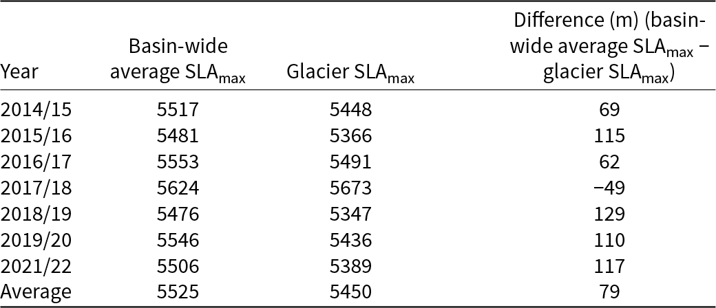
Here we present the fluctuation of the basin-wide average SLAs for the Dudh Koshi basin and glacier SLAs for Mera Glacier over the period 2015–23 (Fig. 7a). Over the Dudh Koshi basin, basin-wide average SLAs ranged from 5090 ± 36 m in 2020 to 5624 ± 23 m in 2018. A total of 68 glacier SLAs were detected on Mera Glacier, ranging from 5168 ± 21 m in 2020 to 5673 ± 25 m in 2018. The number of basin-wide average SLAs and glacier SLAs detected varied annually depending on the sensor, as well as cloud cover and surface conditions (Fig. 7a and Supplementary Table S2). SLAmax usually occurs after November and as late as January of the next year. The annual basin-wide average SLAmax and glacier SLAmax for Mera Glacier are given in Table 2 and also shown with sub-monthly basin-wide average SLAs in Fig. 7a and Supplementary Table S2.
(a) Remote-sensing basin-wide average SLAs for Dudh Koshi basin (blue) and glacier SLAs for Mera Glacier (purple) over the period 2015–23. SLAmax values are marked in red for Dudh Koshi basin and yellow for Mera Glacier. The span of field measurement dates is shown as gray vertical bars with field-based ELAs as a horizontal black line at top, and the x-Axis displays the dates of field measurements and hydrological years; (b) scatter plot of basin-wide average SLAs vs Glacier SLAs on common dates over the study period.

Figure 7 Long description
The image consists of two parts: (a) A graph showing snowline altitudes in meters above sea level for the Dudh Koshi basin and Mera Glacier from 2015 to 2023. The x-axis represents hydrological years, while the y-axis shows snowline altitudes. Blue dots represent SLA for Dudh Koshi, red dots for Max SLA Dudh Koshi, purple dots for SLA Mera and yellow dots for Max SLA Mera. Grey vertical bars indicate field measurement dates and a black horizontal line shows field-based ELA for Mera. (b) A scatter plot comparing SLA for Dudh Koshi (x-axis) and SLA Mera (y-axis) with a linear equation Y equals 1.04X minus 327.04 and a correlation coefficient r equals 0.81.
Basin-wide average SLAmax and glacier SLAmax (Mera Glacier) for each hydrological year over the period 2015–23 and averages over the entire period.

Table 2 Long description
The table compares the basin-wide average SLAmax and the Mera Glacier SLAmax for each hydrological year from 2015 to 2023, along with their differences. The basin-wide average SLAmax consistently exceeded the glacier SLAmax, except in 2017/18 when the glacier SLAmax was 49 meters higher. The largest positive difference occurred in 2018/19, with the basin-wide average being 129 meters higher than the glacier SLAmax. The average difference over the entire period was 79 meters. These variations highlight the differences in snow line altitudes between the basin-wide average and the specific glacier, indicating potential influences of local climatic or environmental factors.
Basin-wide average SLAmax ranged from 5476 ± 24 m in 2019 to 5624 ± 23 m in 2018, averaging 5525 ± 23 m over the entire period 2015–23 (Table 2, Fig. 7a). Glacier SLAmax ranged from 5347 ± 22 m in 2019 to 5673 ± 25 m in 2018, averaging 5450 ± 21 m over the entire period (Table 2, Fig. 7a). The years with the lowest and highest SLAmax (2019 and 2018, respectively) were consistent between the basin-wide average SLAmax and glacier SLAmax, although glacier SLAmax were on average ∼79 m lower than basin-wide average SLAmax (Table 2). The comparison between glacier SLAs and basin-wide average SLAs shows a good agreement (Pearson’s r = 0.81), indicating that the glacier SLA of Mera Glacier is representative of basin-wide average SLA (Fig. 7b). Estimated basin-wide average SLAs are within the range of SLAs reported in a previous study for the same basin by Racoviteanu and others (Reference Racoviteanu, Armstrong and Williams2013) (5172–6047 m, mean ELA = 5568 m) based on analysis of December 2005 imagery. Our results are also in agreement with contemporary ELAs reported in Owen and Benn (Reference Owen and Benn2005) for the same region (5200–5800 m, with a mean value of 5600 m).
4. Discussion
4.1. Intra- and interannual SLA trends
The intra- and interannual variability of SLAs gives insights into the temporal behavior of SLAs in a monsoon-dominated region. Intra-annual SLA evolution within each hydrological year showed generally increasing patterns from April to November, but our results show that none of the trends were statistically significant for either basin-wide average SLA or glacier SLA (Mera Glacier), assessed using the Mann–Kendall test with 95% confidence level (p > 0.05). The SLA on Mera Glacier as detected using the satellite images often continues to rise after the field measurement dates (i.e. November). Basin-wide average SLAmax and glacier SLAmax did not occur on same dates every year but rather late in the post-monsoon to early winter months (December or even in January) which belong to the next hydrological year (Fig. 7a). This is consistent with the previous studies, which suggested that the SLA observed in post-monsoon or winter months reflects the previous ablation season due to the wind erosion, snow redistribution and sublimation (Wagnon and others, Reference Wagnon2013; Brun and others, Reference Brun2015). We found no significant trends in interannual basin-wide average SLAmax and glacier SLAmax over the study period, based on Mann–Kendall test with 95% confidence level (p > 0.05). While our results show considerable intra-annual variability in SLA and interannual variability in SLAmax, we did not find a statistically significant trend in SLA/SLAmax over the study period. The relatively short period of observation (7 years) does not allow us to make solid conclusions about long-term trends.
4.2. Discrepancies between the remote-sensing SLAs and the field-based ELAs
When comparing field-based ELA and remote-sensing SLA of Mera Glacier taken on concomitant dates at the end of the ablation season (i.e. November), we obtained large differences ranging from 161 m for the 2017/18 hydrological year to 508 m for 2021/22 (Fig. 7). The average remote-sensing SLA over the period 2015–23 (5377 ± 26 m) was ∼400 m lower than average field-based ELA (5739 m) estimated using the traditional glaciological method (Wagnon and others, Reference Wagnon2021). These large differences persisted to some extent when comparing SLAmax values (generally occurring at a later date i.e., December) with field-based ELAs for all the hydrological years except the year 2014/15 (5 m difference) (Table 3 and Fig. 7a). However, these were smaller (up to 435 m in 2018/19) than those based on concomitant SLAs and field-based ELAs as mentioned above. These mismatches suggest that the remote-sensing SLAs (and even SLAmax) do not fully capture the true ELA on Mera Glacier.
Comparison of remote-sensing (Sentinel-2/Landsat 8 [S2/L8] and Planet/VENμS) SLAmax with field-based ELAs for Mera Glacier over the period 2015–23, extracted from AW3D30 (30 m) and HMA (8 m) DEMs.

Table 3 Long description
The table compares field-based equilibrium line altitudes (ELA) with remote sensing snow line altitudes (SLAmax) for Mera Glacier from 2015 to 2023. Field observations were conducted annually, with the highest ELA recorded in 2021/22 at 5817 meters. Remote sensing data from Sentinel-2/Landsat-8 and Planet/VENμS show variations in SLAmax, with differences in measurements from AW3D30 and HMA digital elevation models (DEMs). Notably, the 2017/18 and 2021/22 years lack Planet/VENμS data. The data reveal discrepancies between field-based and remote sensing measurements, highlighting the challenges in aligning these methods. Trends indicate fluctuating altitudes, with no consistent pattern of increase or decrease over the observed period.
To check for potential biases in the remote-sensing SLAs, we evaluated the impact of spatial resolution and the choice of DEM. The comparison of SLAmax estimated from Sentinel-2/Landsat 8 images and high-resolution imagery on the same or nearby date (1 or 2 days) showed no significant differences (Table 3). Similarly, a sensitivity analysis of remote-sensing SLAs to the choice of DEM (AW3D30 DEM, 30 m spatial resolution vs HMA DEM, 8 m) yielded only ∼35 m difference in the remote-sensing SLAs (Table 3). This is roughly ten times smaller than the mean difference of ∼400 m between remotely sensed SLA and field-based ELA (2015–23). This shows that the choice of DEM did not significantly influence the large negative bias in the remote-sensing SLA values, indicating that other surface processes are at play on monsoon-dominated glaciers, thus contributing to the low remote-sensing SLAs/SLAmax.
We hypothesize that the systematic mismatch between the concomitant SLAs (i.e. SLAs extracted from images acquired during the field measurement period, generally November) and field-based ELAs on Mera Glacier is due to either snow persisting from the monsoon or snowfall events occurring at the end of the ablation season, or a combination of both. Mera Glacier, being a summer-accumulation-type glacier, receives snowfall throughout the summer. While most of this snow is expected to melt during the monsoon due to higher temperatures, thus exposing the glacier ice over the ablation area, some snow can persist throughout the post-monsoon. Similarly, any snowfall occurring in October and November (when temperatures are generally much lower) is more likely to persist on the glacier surface. Furthermore, throughout the period October to April, snow is systematically redistributed from the higher altitudes by the strong winds (Wagnon and others, Reference Wagnon2013). The combination of snow persistence and snow redistribution most likely contributes to the systematically lower SLAs compared to field-based ELAs observed at the end of the ablation season. As a result, in most years, the maximum SLA (∼ELA) may not occur until later in the winter or the following year, before the melting season starts (Brun and others, Reference Brun2015).
To support this hypothesis, we examined field measurements (snow depths and point mass balance) on Mera Glacier. Field measurement data showed snow persistence during the November field campaigns, even below the ELA (Table 4). In most years, glacier areas within the 5400 – 5600 m elevation band showed negative mass balances; yet, by the end of the ablation season, these areas remained snow-covered, with average snow depth ranging from ∼15 cm (2019/20) to ∼72 cm (2020/21) (an overall mean of ∼37 cm) except in 2017/18, when snowfall was minimal (a dry year). Consistent with our hypothesis that late-season/persistent snowfall drives the SLA-ELA difference, the 2017/18 hydrological year showed the smallest discrepancy between the remotely sensed SLA and the field-based ELA (161 m) (Fig. 7a), likely due to minimal snowfall over the glacier surface during October–November, just prior to field measurements. We could not compare SLA with field-based ELA in 2020/21 because the glacier was completely snow-covered following the typhoon event.
Average snow depth H (cm) and mean altitudinal mass balance b a (m w.e.) on Mera Glacier for the hydrological years over the period 2015–23.

Table 4 Long description
The table presents average snow depth and mean altitudinal mass balance on Mera Glacier from 2015 to 2023, focusing on elevations above 5400 meters. Snow depth varied, peaking at 72 cm in 2020/21 at 5400–5500 meters, while the lowest recorded was 0 cm in 2017/18. The altitudinal mass balance was predominantly negative, indicating a loss in mass, with the most negative value of -1.4 in 2021/22 at 5400–5500 meters. Notably, data for some years and elevations are missing, marked as 'N/A', which may affect trend analysis. Overall, the data suggests fluctuating snow depth and a general trend of mass loss over the years.
Note: Ablation stake measurements were averaged per 100 m elevation bin at altitudes above 5400 m. ‘N/A’ indicates unreported or missing data.
The ELA-SLA findings also imply there is no superimposed ice. Superimposed ice can be deposited due to refreezing of meltwater—at elevations between the equilibrium line and the firn line (Lliboutry, Reference Lliboutry, Williams and Ferrigno1998), but it can also be found underneath the snow of the current year at elevations above the snowline and subsequently get exposed. However, superimposed ice adds mass to the glacier and would cause the ELA to be situated below the SLA at the end of ablation season, which is not the case here. However, recent research, for example, in the Tien Shan showed that this ELA-SLA relationship in the presence of superimposed ice depends on the melting pattern (Yuwei and others, Reference Yuwei, Jianqiao, Zhongming and Anan2014; Yue and others, Reference Yue, Li, Zhao, Li, Wang and Wang2021). In the case of Mera, wind scouring rather than intense melting would expose the superimposed ice zone. As Mera experiences mostly negative mass-balance, if ablation reaches the firn layer from the previous year, the remote-sensing SLA is detected as the lower boundary of the firn layer from the previous year (Yuwei and others, Reference Yuwei, Jianqiao, Zhongming and Anan2014), while the true ELA is above. Even though later in the ablation season, the snowline may retreat beyond the firnline, the optical satellite imagery will still detect the firnline rather than the snowline. This combination of melting patterns and wind scouring could partially explain the large difference in SLAmax and the field-based ELA on Mera Glacier.
The analysis of Mera Glacier suggests that comparing satellite-derived SLAs with field-based ELAs is particularly challenging in monsoon-dominated regions. In such regions, late-summer snowfall often persists on the glacier surface due to lower temperatures, leading to systematically lower SLAs compared to field-based ELAs. This is evident from the significant discrepancies observed on Mera Glacier and on other glaciers in the Tian Shan and tropical regions (Rabatel and others, Reference Rabatel2012; Yuwei and others, Reference Yuwei, Jianqiao, Zhongming and Anan2014). In these regions, due to simultaneous ablation and accumulation processes, remote-sensing SLAs do not accurately capture the true ELA, suggesting that the assumption that SLAmax ≈ ELA does not hold in such regions. These findings indicate that the SLA-ELA mismatch is primarily controlled by the climatic regime rather than limitations in optical snowline extraction alone. Although denser temporal sampling better captures snowline dynamics, surface processes prevent a consistent correspondence between SLAmax and ELA under monsoon conditions. Future integration of complementary datasets, such as synthetic aperture radar, may further improve snowline detection under persistent cloud cover and the presence of snow, but this needs thorough investigations, which are beyond the scope of the current study.
4.3. Improved SLA extraction: significance and limitations
The proposed SLA extraction method was able to capture the temporal evolution of SLAs at the basin scale across multiple seasons, providing a clear view of SLA dynamics throughout the hydrological year. This method not only allows the detection of SLAs throughout the ablation season but also facilitates the identification of the date of the SLAmax. By applying a consistent, semiautomated approach, we developed a robust temporal SLA dataset, which was critical for understanding SLA behavior and testing the SLA-ELA relationship.
The proposed method provides promising results, yielding overall very small differences in means of SLAs when compared to those extracted from high-resolution satellite data (Table 1). However, these differences do vary on a year-by-year basis (Sentinel-2: 1.06–23.95 m; Landsat 8: 4.36–9.74 m) depending on cloud cover and the quality of images (shadows, etc.). Overall, results obtained at basin scale showed good agreement with the manually delineated SLAs at glacier scale (Fig. 4). The automated filtering procedure based on the negative buffer, box plot and sieve filter proposed in this study effectively minimized the outliers around the ridgelines as well as in the accumulation and ablation areas, with challenges remaining in different topographic settings (Fig. 6).
While the present method shows potential for efficiently detecting SLAs, it is nevertheless subject to the limitations of optical data, that is, persistent cloud cover in the central-eastern region of the Himalaya during the monsoon. Therefore, in such areas, the use of other types of data, such as synthetic aperture radar, which are not affected by clouds, should be tested (Garg and others, Reference Garg, Thakur, Rajak, Aggarwal and Kumar2022). In the monsoon-dominated areas, any (semi) automated method is challenged by the presence of snow, which may cover the snowlines, as discussed above. Furthermore, the oversaturation issue due to highly reflective surfaces (i.e. bright snow) and stripping due to scanline corrector failure in Landsat 7 (ETM+) (USGS, 2024) are general sources of uncertainties in optical data, but they did not affect this study, which used Landsat 8. In this study, we have quality-controlled the image selection step as much as possible to minimize the effect of these issues.
5. Summary and conclusions
This study investigated the sub-monthly SLAs at multi-scale (basin to glacier scale) over a monsoon-dominated area of the Himalaya over the period 2015–23 using optical remote sensing. Our study highlights some important findings.
First, the SLA extraction with an added post-processing filtering represents a robust approach for identifying glacier SLAs from satellite data such as Landsat 8 and Sentinel-2, thanks to the addition of Otsu thresholding and an automated filtering procedure. It has the advantage of using only limited input data (a freely available global DEM and multi-sensor satellite images), making it suitable for application to multi-spatial scales, from glacier to basin scale. The automated filtering procedure implemented in this study is an advancement over the previous semiautomated SLA delineation routine, as it enhances the reliability of SLA estimates by minimizing errors due to shadows, crevassed areas, snow patches, etc. It provided high accuracy when compared to SLAs estimated from high-resolution data despite a few remaining outliers. Prospective improvements to separate snow and ice include the addition of more sophisticated methods based on spectral unmixing (Painter and others, Reference Painter, Rittger, McKenzie, Slaughter, Davis and Dozier2009; Racoviteanu and others, Reference Racoviteanu, Nicholson and Glasser2021), machine learning-based classification for glacier surfaces and/or integration of the method in the Google Earth Engine platform (Loibl and others, Reference Loibl, Richter and Grünberg2025). Even if in this study we implemented and tested the method on a single basin/single glacier, the workflow is flexible and can be used for other basins if the images are cloud-free. This holds potential for investigating snowline evolution throughout the year from glacier to basin scale.
Second, using Mera Glacier as a case study, we challenged the assumption that SLAmax is an appropriate proxy for ELA in this area. Based on the systematic discrepancies noted (SLAmax < ELA), we hypothesized the presence of snow obscuring the ELA, which we confirmed based on field-based measurements. Overall, our findings emphasize the complexity of snowline dynamics in monsoon-dominated regions where simultaneous accumulation and ablation and various surface processes, including sublimation, wind-driven snow redistribution and seasonal snow cover, pose challenges for SLA detection. We conclude that the assumption that SLAmax ≈ ELA does not hold in these regions. Therefore, SLA-derived ELAs based on this assumption should be used with caution and carefully checked when inferring glacier mass balance.
Supplementary material
The supplementary material for this article can be found at https://doi.org/10.1017/jog.2026.10169.
Data availability statement
The Python code for the developed semiautomated method is open source and is available at https://github.com/Semi-automated/Semi-automated-Snowline-estimation.git.
Acknowledgements
M.F.A. acknowledges the research grants from SERB (CRG/2020/004877), Space Application Centre (SAC, ISRO) and MoES (MOES/PAMC/HC/131/2019-PC-II). A.R. acknowledges support from the NASA 80NSSC20K1721 project in the initial phase of this work as well as the French IRD and the GLACIOCLIM network for field logistics and access to field data. We acknowledge the USGS Earth Explorer and Copernicus for providing free access to Landsat series and Sentinel-2 datasets; Planet Labs Inc., for providing access to the Planet imagery through their API 332 program and the French CNES for providing free access to VENμS imagery. We thank F. Brun and A. Rabatel (IGE, Grenoble, France) for the exchanges during the preparation of this work.
Author contributions
A.R. conceptualized the initial semiautomated method; P.V. refined the method and ran the image processing, Python code and validation with input from M.F.A. and A.R. A.R. performed the manual delineation of SLAs on high-resolution images and provided the 2020 glacier mask. P.V. developed the figures and wrote the paper with input from A.R. and M.F.A.




 Open access

