





1. Introduction
Wall-shear stress is a fundamental quantity in wall-bounded turbulence and its accurate measurement is crucial for advancing both fundamental and applied fluid dynamics (Winter Reference Winter1979). Instantaneous and spatially resolved wall-shear stress measurements provide direct information about the near-wall cycle of turbulence production and bursting processes (Kline et al. Reference Kline, Reynolds, Schraub and Runstadler1967; Blackwelder & Kaplan Reference Blackwelder and Kaplan1976; Blackwelder & Haritonidis Reference Blackwelder and Haritonidis1983), and they are essential for quantifying the interaction between near-wall streaks and large-scale structures (Abe et al. Reference Abe, Kawamura and Choi2004; Schlatter et al. Reference Schlatter, Örlü, Li, Brethouwer, Fransson, Johansson, Alfredsson and Henningson2009; Schlatter & Örlü Reference Schlatter and Örlü2010b ; Chen et al. Reference Chen, Iwano, Sakai and Ito2021; Chernyshenko Reference Chernyshenko2021). Hutchins et al. (Reference Hutchins, Monty, Ganapathisubramani, Ng and Marusic2011) used conditional sampling of hot-film signals in air flows in combination with velocity measurements to reveal the three-dimensional structure of large-scale motions and their footprint on the wall. Pabon et al. (Reference Pabon, Ukeiley, Sheplak and Barnard Keane2018) employed micro-electro-mechanical-systems (MEMS) based sensors in air flows to directly capture fluctuating wall-shear stress in turbulent boundary layers and investigated its correlation with large-scale motions. More recently, Örlü & Vinuesa (Reference Örlü and Vinuesa2020) reviewed advances in instantaneous wall-shear stress measurements, emphasising their application in identifying near-wall extreme events such as backflow and super-streaks. Such measurements have also been employed to investigate transitional flows, where hot-film sensors were used to identify the onset of turbulence in a quantitative manner (Whalley et al. Reference Whalley, Park, Kushwaha, Dennis, Graham and Poole2017). Detailed spatio-temporal studies further highlighted the role of intermittent low-drag and hibernating events in transitional and low-Reynolds-number turbulence, reinforcing the importance of time-resolved wall-shear stress data (Whalley et al. Reference Whalley, Park, Kushwaha, Dennis, Graham and Poole2017, Reference Whalley, Dennis, Graham and Poole2019). In engineering applications, wall-shear stress is central to skin-friction drag reduction, where accurate instantaneous measurements can provide insight into the physical mechanisms underlying flow control strategies (Whalley & Choi Reference Whalley and Choi2014; Mahfoze & Laizet Reference Mahfoze and Laizet2017; Mahfoze et al. Reference Mahfoze, Moody, Wynn, Whalley and Laizet2019; Chen et al. Reference Chen, Iwano, Sakai and Ito2022). These examples demonstrate that reliable measurements of wall-shear stress are not only vital for understanding fundamental turbulence mechanisms but also hold significant potential for enabling effective flow control strategies.
Early attempts to quantify the fluctuating wall-shear stress were based on near-wall velocity measurements, relying on the similarity between wall-shear stress fluctuations and streamwise velocity fluctuations within the viscous sublayer (Eckelmann Reference Eckelmann1974; Alfredsson et al. Reference Alfredsson, Johansson, Haritonidis and Eckelmann1988; Marusic & Heuer Reference Marusic and Heuer2007; Örlü et al. Reference Örlü, Fransson and Alfredsson2010; Alfredsson et al. Reference Alfredsson, Örlü and Schlatter2011), and applying Newton’s law of viscosity,
 $\tau = \mu ( {\partial u}/{\partial y}) \approx \mu ( {{\rm d}u}/{{\rm d}y})$
, for
 $y^+\lt 5$
. Here,
 $\tau$
denotes the wall-shear stress,
 $\mu$
is the shear viscosity and the superscript ‘
 $+$
’ indicates viscous scaling, i.e.
 $y^+ = y u_\tau / \nu$
, where
 $u_\tau$
is the friction velocity and
 $\nu$
is the kinematic viscosity. Thermal anemometry was among the first technique employed to estimate velocity gradients and wall-shear stress fluctuations in this region (Eckelmann Reference Eckelmann1974; Alfredsson et al. Reference Alfredsson, Johansson, Haritonidis and Eckelmann1988; Ruedi et al. Reference Ruedi, Nagib, Österlund and Monkewitz2003, Reference Ruedi, Nagib, Österlund and Monkewitz2004), followed by laser Doppler velocimetry (LDV), which enabled the acquisition of time-resolved statistics within the viscous sublayer (Durst et al. Reference Durst, Jovanović and Sender1995). More recently, optical approaches such as particle image velocimetry (PIV) and micro-particle tracking velocimetry (
 $\mathrm{\mu PTV}$
) have been applied to recover wall-shear stress information with improved spatial resolution (Li et al. Reference Li, Jessen, Roggenkamp, Klaas, Silex, Schiek and Schröder2015, Reference Li, Roggenkamp, Jessen, Klaas and Schröder2017; Willert Reference Willert2015). In addition, micro-pillar sensors have been developed to infer near-wall shear indirectly from the deformation of flexible pillars exposed to the viscous sublayer flow (Große & Schröder Reference Große and Schröder2008; Gnanamanickam et al. Reference Gnanamanickam, Nottebrock, Große, Sullivan and Schröder2013; Brücker Reference Brücker2015). In parallel, a number of techniques have been developed to access the wall-shear stress directly. For instance, Heuer and Marusic developed a large-scale floating-element wall-shear stress balance (Heuer & Marusic Reference Heuer and Marusic2005; Marusic & Heuer Reference Marusic and Heuer2007), Baars et al. (Reference Baars, Squire, Talluru, Abbassi, Hutchins and Marusic2016) demonstrated accurate wall-drag measurements in smooth- and rough-wall boundary layers using a similar large-scale balance, while Ferreira et al. (Reference Ferreira, Rodriguez-Lopez and Ganapathisubramani2018) proposed an alternative floating-element design with improved accuracy and reliability. While these methods show promise, their application in aerodynamic facilities is often restricted by spatial resolution limits, installation complexity or frequency-response constraints. For MEMS-based floating-element devices, Schmidt et al. (Reference Schmidt, Howe, Senturia and Haritonidis1988) first developed a microfabricated capacitive floating-element sensor for turbulent boundary layers, demonstrating the feasibility of direct wall-shear stress measurement. Subsequent studies, such as those by Sheplak et al. (Reference Sheplak, Cattafesta, Nishida and McGinley2004), Pabon et al. (Reference Pabon, Ukeiley, Sheplak and Barnard Keane2018) and Liu et al. (Reference Liu, Wang, Ding, Zhang, Deng, He, Ma and Yuan2025), further advanced the design, calibration and application of MEMS-based sensors for dynamic wall-shear stress measurements. However, these sensors remain susceptible to fabrication complexity, packaging difficulties and long-term stability issues, which limit their widespread use in turbulent air-flow experiments. As a result, flush-mounted hot-film probes have remained the most widely used sensors for turbulent flows, since they provide a practical means of resolving time-resolved wall-shear stress without relying on assumptions of sublayer similarity. In liquid flows, such as in water (Madavan et al. Reference Madavan, Deutsch and Merkle1985) or more recently in glycerine–water mixtures (Whalley et al. Reference Whalley, Park, Kushwaha, Dennis, Graham and Poole2017, Reference Whalley, Dennis, Graham and Poole2019), flush-mounted hot-film probes have been shown to provide accurate measurements of instantaneous wall-shear stress. However, when applied in air flows, their performance is limited by substantial heat conduction into the substrate, which leads to a systematic underestimation of the wall-shear stress fluctuations when using a standard calibration approach (Eckelmann Reference Eckelmann1974; Alfredsson et al. Reference Alfredsson, Johansson, Haritonidis and Eckelmann1988; Hutchins et al. Reference Hutchins, Monty, Ganapathisubramani, Ng and Marusic2011; Whalley et al. Reference Whalley, Dennis, Graham and Poole2019). Here, standard calibration refers to the conventional multi-point approach where a relationship is established between the hot-film voltage and the mean wall-shear stress, determined from the mean streamwise velocity gradient from within the viscous sublayer across various free-stream velocities.
To address the underestimation of wall-shear stress fluctuations inherent in flush-mounted hot-film probes when applied in air flows, the present study adopts a nonlinear regression (NLR) approach. While NLR has previously been applied to mitigate calibration drifts in thermal anemometry, for instance, those caused by variations in ambient conditions (Agrawal et al. Reference Agrawal, Whalley, Ng, Dennis and Poole2019), it is here extended to turbulent air flows to recover accurate instantaneous wall-shear stress measurements. The wall-shear stress
 $\tau$
is formulated as a polynomial function of the hot-film output voltage
 $E$
, and the calibration is constrained through statistical moments obtained either from LDV in the viscous sublayer or from direct numerical simulations (DNS) at matched Reynolds numbers. The approach demonstrates that calibration can be reliably achieved using only the first statistical moment from the same flow, while the higher-order moments can be supplied from DNS or estimated from their Reynolds-number dependence. This development provides, for the first time, a practical means of correcting the attenuation inherent in hot-film measurements and enables accurate instantaneous wall-shear stress data to be obtained in turbulent air flows. The paper is organised as follows. Section 2 describes the experimental set-up, including the wind-tunnel facility, the LDV system and the hot-film system. Section 3 presents the global flow characterisation measured by LDV and the comparison with DNS. Section 4 introduces the NLR framework used for calibrating each hot film. Sections 5–7 introduce three different approaches for obtaining the moments required for the NLR technique to calibrate the hot films and examine the resulting calibration performance. Sections 8 and 9 present two case studies to demonstrate the applicability of the method to historical datasets and the additional physical insights that can be extracted from them. Section 10 provides a discussion on the implications of the method with conclusions provided in § 11.
2. Experimental set-up
The experiment was performed in an open-return boundary-layer wind tunnel at Newcastle University. The maximum free-stream speed of the facility is 30 m s−1, with a test section of 0.46 m in width and 0.32 m in height. The flat plate used to develop the turbulent boundary layer is
 $L_{\textit{plate}} = 3.5$
m long and is equipped with a trailing-edge flap for flow conditioning. A zigzag trip was installed 100 mm downstream of the sharp leading edge across the full width of the flat plate to promote transition to turbulence. The trip has a height of 1.5 mm and a streamwise length of 10 mm (Elsinga & Westerweel Reference Elsinga and Westerweel2012). The free-stream turbulence intensity was found to be approximately 0.3 % after applying a band-pass filter, with the high-pass cutoff frequency defined as
 $f_{h} = U_{\infty } / (2L_{\textit{plate}})$
(Cattafesta et al. Reference Cattafesta, Bahr and Mathew2010) and the low-pass cutoff set at
 $f_{l} = 5000$
Hz to remove high-frequency noise from the measurement circuit, as verified through preliminary hot-wire measurements conducted prior to the main experiment. Here,
 $U_\infty$
indicates the free-stream velocity. A summary of the experimental conditions is given in table 1. Throughout the paper,
 $x$
,
 $y$
and
 $z$
denote the streamwise, wall-normal and spanwise directions, respectively. Lowercase letters indicate instantaneous components. An overbar denotes time-averaged quantities, for example,
 $\overline {u}$
for time-averaged streamwise velocity. A prime denotes fluctuating components, e.g.
 $\tau '=\tau -\overline {\tau }$
. The root-mean-square or second moment value is written as
 $\sigma$
, e.g.
 $\sigma (\tau )$
, while higher-order statistical moments are given by
 $S$
for skewness (third moment) and
 $F$
for kurtosis (fourth moment). The boundary-layer thickness
 $\delta$
is defined as the wall-normal location where the time-averaged streamwise velocity reaches
 $0.99U_\infty$
. The slight non-monotonic variation of
 $\delta$
in table 1 is attributed to the uncertainty associated with the
 $0.99U_\infty$
threshold definition. The momentum thickness is denoted by
 $\theta$
. The Reynolds numbers based on the friction velocity and momentum thickness are calculated as
 $\textit{Re}_\tau = u_\tau \delta /\nu$
and
 $\textit{Re}_\theta = \theta U_\infty /\nu$
, respectively. For any dimensional length
 $L$
, the corresponding viscous-scaled quantity is defined as
 $L^+ = {L u_\tau }/{\nu }$
. The uncertainty of a flow quantity
 $Q$
is denoted by
 $\varepsilon _Q$
. To assess the uncertainties of the estimated friction velocity
 $u_\tau$
and wall-normal position
 $y$
, a standard least-squares linear regression was applied to the viscous sublayer data (
 $y^+ \lt 4.5$
), following the method of Hutchins & Choi (Reference Hutchins and Choi2002). For other quantities that are functions of independent variables, such as
 $\textit{Re}_\tau = u_\tau \delta /\nu$
, the corresponding uncertainties were estimated using the error-propagation method of Kline & McClintock (Reference Kline and McClintock1953). The resulting uncertainties of the key flow quantities are summarised in table 2.
A summary of the experimental conditions.

Table 1. Long description
The table presents a summary of experimental conditions for a boundary-layer wind tunnel experiment. It contains 3 rows and 12 columns. The columns are labelled as follows: U infinity in m s^-1, u tau in m s^-1, delta in mm, theta in mm, Re tau, Re theta, l plus R45, w plus R45, l plus R47, w plus R47, D plus LDV, and l plus LDV. The rows provide specific values for each of these parameters. Row 1: 6.11, 0.253, 39.4, 5.40, 664, 2200, 12.6, 3.4, 15.2, 1.7, 0.73, 5.4. Row 2: 8.06, 0.327, 39.7, 5.32, 863, 2860, 16.3, 4.4, 19.6, 2.2, 0.94, 7.0. Row 3: 10.76, 0.422, 36.7, 5.02, 1032, 3600, 21.1, 5.6, 25.3, 2.8, 1.21, 9.0. The table provides detailed measurements and conditions for the experiment, including free-stream velocity, friction velocity, boundary-layer thickness, momentum thickness, Reynolds numbers, and hot-film and LDV probe dimensions in viscous units.
Uncertainty estimates of the experimental parameters.

Table 2. Long description
A table with uncertainty estimates of experimental parameters. The table has three rows and eight columns. The column headers are epsilon_U_infinity in m s^-1, epsilon_u_tau in m s^-1, epsilon_y in micrometres, epsilon_delta in mm, epsilon_theta in mm, epsilon_Re_tau, epsilon_Re_theta, and epsilon_L_plus_equals_1. Row 1: 0.004, 0.002, 2.4, 0.2, 0.02, 6, 24, 0.012. Row 2: 0.008, 0.006, 6.3, 0.6, 0.13, 21, 74, 0.022. Row 3: 0.006, 0.006, 3.9, 0.3, 0.06, 16, 53, 0.017.
Schematic of the experimental set-up.

Velocity measurements were obtained using an LDV system and were performed approximately 1800 mm downstream of the zigzag trip, where the boundary layer was fully developed. A COHERENT Genesis MX514-1000 SLM laser system with a power output of 300 mW was used as the laser source. Two laser beams with a wavelength of 488 nm (blue) outlined a plane parallel to the wall and were used to measure the streamwise velocity component. The transmitting and receiving optics were mounted on opposite sides of the wind tunnel, as shown in figure 1. The optical system for emitting the laser had a focal length of 480 mm and a beam expander (TSI, Model XPD60) with an expansion ratio of 2.6 was used to achieve a final beam diameter of 2.65 mm. The beam spacing for the laser was 50 mm. The nominal measurement volume had a diameter of
 $D_{\textit{LDV}} = 0.043$
mm and a length of
 $l_{\textit{LDV}} = 0.32$
mm, with the corresponding viscous-scaled dimensions summarised in table 1. The LDV signals were processed using a 16-bit Dantec Burst Spectrum Analyser (BSA-F60). The traverse stages provide a positioning resolution of 12.5
 $\mathrm{\unicode{x03BC} m}$
on the laser side and 0.625
 $\mathrm{\unicode{x03BC} m}$
on the receiver side in the wall-normal direction. The seeding particles were olive oil droplets with a nominal diameter of 1
 $\mathrm{\unicode{x03BC} m}$
, yielding a Stokes number less than 0.1 to ensure faithful tracking of the flow (Tropea et al. Reference Tropea2007). The sampling frequency varied from approximately 8 kHz in the free stream to 500 Hz near the wall, and data were acquired for 90 s to achieve statistical convergence.
Wall-shear stress measurements were obtained using two types of hot-film probes, which were tested separately: a Dantec 55R45 flush-mounted sensor (
 $l \times w = 0.75 \times 0.2$
mm) and a Dantec 55R47 glue-on sensor (
 $l \times w = 0.9 \times 0.1$
mm). To ensure flush mounting, hot-film sensors (models 55R45 and 55R47) were seated in pre-machined recesses. Dial gauge verification showed a maximum surface deviation of
 $20\ \unicode{x03BC} \text{m}$
, keeping the sensors within
 $y^+ \lt 0.57$
for the entire Reynolds-number range. Both sensors were operated with a Dantec StreamLine Pro constant-temperature anemometer, set with an overheat ratio of 1.5. The analogue outputs were acquired through a National Instruments system consisting of a BNC-2110 terminal block and a PXIe-6356 high-speed data acquisition card. The sampling frequency was 20 kHz with a recording duration of 90 s for each condition. Tests were performed at three free-stream velocities of 6.1, 8.1 and 10.8 m s−1.
Viscous-scaled wall-normal profiles of boundary-layer properties: (a) time-averaged streamwise velocity
 $\overline {u}^+$
, (b) streamwise turbulent intensity
 $\sigma ({u'}^+)$
.

Figure 2. Long description
The image contains two line graphs labeled as Panel A and Panel B. Panel A: This line graph shows the viscous-scaled wall-normal profiles of the time-averaged streamwise velocity. The x-axis is labeled y+ and ranges from 10^0 to 10^3. The y-axis is labeled u+ and ranges from 0 to 30. The graph includes multiple data series represented by different symbols and colors: blue circles for experimental data with U∞ = 6.1 m/s and Reθ = 2200, orange circles for experimental data with U∞ = 8.1 m/s and Reθ = 2860, and yellow circles for experimental data with U∞ = 10.8 m/s and Reθ = 3600. Additionally, there are lines representing DNS data with Reθ = 2200, DNS data with Reθ = 2400 by Schlatter et al. (2009), and theoretical lines for U+ = y+ and U+ = (1/0.385) ln(y+) + 4.9. An inset within Panel A shows a zoomed-in view of the lower y+ range. Panel B: This line graph shows the viscous-scaled wall-normal profiles of the streamwise turbulent intensity. The x-axis is labeled y+ and ranges from 10^0 to 10^3. The y-axis is labeled σ(u+). The graph includes the same data series and lines as Panel A, showing how the streamwise turbulent intensity varies with y+.
3. Global flow characterisation
Wall-normal profiles of the turbulent boundary layer were obtained from both LDV measurements and DNS performed using the high-order finite-difference solver Xcompact3D (Bartholomew et al. Reference Bartholomew, Deskos, Frantz, Schuch, Lamballais and Laizet2020), which has been extensively validated in previous studies of zero-pressure-gradient turbulent boundary layers (Diaz-Daniel et al. Reference Diaz-Daniel, Laizet and Vassilicos2017; Mahfoze & Laizet Reference Mahfoze and Laizet2021; O’Connor et al. Reference O’Connor, Diessner, Wilson, Whalley, Wynn and Laizet2023, Reference O’Connor, Laizet, Wynn, Edeling and Coveney2024; Wynn et al. Reference Wynn, Parvar, O’Connor, Frantz and Laizet2025). All LDV statistics were computed with transit-time weighting of the seeding particles (Buchhave et al. Reference Buchhave, George and Lumley1979; Tropea Reference Tropea1995). For consistency, the profiles were normalised using the friction velocity
 $u_\tau$
, determined by a linear fit of the time-averaged streamwise velocity within the viscous sublayer (
 $y^+ \lt 4.5$
), as shown in the inset of figure 2(a). Figure 2(a) demonstrates that the time-averaged velocity profiles measured by LDV and obtained from DNS collapse well with the DNS data of Schlatter et al. (Reference Schlatter, Örlü, Li, Brethouwer, Fransson, Johansson, Alfredsson and Henningson2009) in both the near-wall and logarithmic regions, despite the different Reynolds numbers. The chosen von Kármán constant
 $\kappa = 0.385$
and additive constant
 $B = 4.9$
provide a reasonable representation of the classical log law (George Reference George2007). Streamwise turbulence intensity profiles, shown in figure 2(b), collapse below
 $y^+=10$
and exhibit a peak around
 $y^+=15$
, consistent with previous observations in high-Reynolds-number boundary layers (Hutchins & Marusic Reference Hutchins and Marusic2007b
; Hutchins et al. Reference Hutchins, Chauhan, Marusic, Monty and Klewicki2012). An increase in outer-layer turbulence intensity with Reynolds number reflects the growing influence of large-scale motions (Hutchins & Marusic Reference Hutchins and Marusic2007a
; Hutchins et al. Reference Hutchins, Nickels, Marusic and Chong2009). Crucially, excellent agreement is observed between LDV measurements at
 $\textit{Re}_\theta = 2200$
and DNS data at the same Reynolds number, confirming both the accuracy of the experimental facility and the suitability of the DNS database for the subsequent NLR calibration. This collapse of experimental and numerical statistics provides confidence in the combined use of LDV, hot-film measurements and high-fidelity DNS in the present study.
4. Nonlinear regression technique
Although the general framework of the NLR technique was introduced by Agrawal et al. (Reference Agrawal, Whalley, Ng, Dennis and Poole2019), the present study employs a constrained form of NLR to ensure a physically admissible calibration. The inputs for this technique are the first four moments of the wall-shear stress time series. The principle of NLR is to adjust the calibration coefficients such that the first four moments of the calibrated hot-film signal match the true moments as closely as possible through an error minimisation process. In the present study, the wall-shear stress
 $\tau$
is represented as a third-order polynomial function of the hot-film output voltage
 $E$
as
 \begin{equation} \tau = aE^3+bE^2+cE+d,\end{equation}
where
 $a$
,
 $b$
,
 $c$
and
 $d$
are the calibration coefficients determined through the NLR optimisation. A fourth-order polynomial was also considered, but the calibration results showed negligible differences compared with the third-order case. Other functional forms, including power-law and exponential representations, were investigated. These formulations substantially increased the computational cost of the NLR process and, in some instances, the algorithm failed to converge to a valid calibration curve. The error function is defined as
 \begin{equation} \epsilon = \left (1 - \frac {\overline {\tau _r}}{\overline {\tau _t}}\right )^2 + \left (1 - \frac {\sigma (\tau _r)}{\sigma (\tau _t)}\right )^2 + \left (1 - \frac {S(\tau _r)}{S(\tau _t)}\right )^2 + \left (1 - \frac {F(\tau _r)}{F(\tau _t)}\right )^2, \end{equation}
where the subscript ‘t’ represents the ‘true’ moments, which are obtained by LDV or DNS in the present study. The subscript ‘r’ represents the moments of the reconstructed wall-shear stress signal measured by the hot-film sensor after the calibration using NLR. To ensure a physically meaningful calibration, a monotonicity constraint was imposed on the polynomial relationship between
 $\tau$
and
 $E$
. In other words, the calibration was constrained such that
 $\tau (E)$
remains strictly monotonic over the entire range of measured voltages. This requirement was enforced by ensuring that
 $\partial \tau /\partial E = 3aE^2+2bE+c$
remains positive or negative throughout the effective range of
 $E$
, depending on whether the hot-film circuit produces a positive or negative response, thereby guaranteeing a one-to-one relationship between
 $\tau$
and
 $E$
. Without such a constraint, the polynomial may become non-monotonic within the measured voltage range, which would imply that multiple voltage values correspond to the same wall-shear stress, a behaviour that is not physically possible for a correctly functioning hot-film circuit.
Comparison of results obtained by different calibration techniques: (a) calibration curves of hot film (55R45), with the inset showing the collapse of 50 calibration curves obtained from different initial guesses of the NLR technique; (b) PDFs of wall-shear stress measured at
 $\textit{Re}_\theta =3600$
.

In the present study the optimal values for the calibration coefficients were calculated using MATLAB’s fmincon function, which is a nonlinear optimisation solver, with initial guesses generated using a random number generator. Since the error function is highly nonlinear, the sensitivity of the calibration to initialisation was examined by generating fifty random sets of initial guesses. The resulting calibration curves collapse almost perfectly within the effective voltage range of the hot film, as shown in the inset of figure 3(a). The average value of the mean absolute percentage error between the instantaneous wall-shear stress signals reconstructed using these fifty calibration curves is 0.13 %. This confirms that the calibration outcome is insensitive to the choice of initialisation and that the constrained NLR procedure consistently converges to an equivalent solution.
5. Nonlinear regression using moments obtained by LDV
In this section the LDV measurements within the viscous sublayer are used to construct an instantaneous wall-shear stress signal, from which the statistical moments serve as inputs to the NLR procedure. Here, the wall-shear stress measured by LDV is calculated as
 $\tau = \mu ({u}/{y}) \big |_{y^+ \lt 5}$
. For context, a standard hot-film calibration is also presented to illustrate its limitations: the amplitude of the instantaneous wall-shear stress is underestimated due to heat conduction into the substrate (Eckelmann Reference Eckelmann1974; Alfredsson et al. Reference Alfredsson, Johansson, Haritonidis and Eckelmann1988; Hutchins et al. Reference Hutchins, Nickels, Marusic and Chong2009; Whalley et al. Reference Whalley, Dennis, Graham and Poole2019). In the standard calibration approach, the time-averaged wall-shear stress is inferred from LDV measurements of the mean streamwise velocity gradient within the viscous sublayer at several free-stream velocities, and these values are plotted against the corresponding time-averaged hot-film voltage, after which the polynomial relationship given in (4.1) is used to establish the mapping between
 $E$
and
 $\tau$
. Since the results obtained using the 55R47 hot-film sensor showed no noticeable differences compared with those from the 55R45 sensor, only one sensor is presented for each result in the following sections for clarity. Figure 3(a) shows the calibration curves obtained by these two different calibration techniques. The yellow solid line represents the result of a standard calibration, with yellow asterisks marking the calibration points. The red solid line represents the NLR calibration result obtained using wall-shear stress moments derived from LDV measurements at
 $y^+ = 3.6$
with
 $U_\infty = 10.8$
m s−1. Compared with the yellow standard calibration curve, the red NLR calibration curve shows that the resulting wall-shear stress is more sensitive to changes in hot-film voltage. Probability density functions (PDFs) of the instantaneous wall-shear stress time series measured by LDV and by the hot film calibrated using the two techniques were also compared, as shown in figure 3(b). The black solid line and red circles represent the results measured by LDV at
 $y^+ = 3.6$
and measured by the hot film calibrated using the NLR technique, respectively. These two PDFs collapse, which indicates that the NLR technique performs as expected, because the similarity in the PDF distribution suggests that the moments of the two time series are nearly the same. Compared with the two PDFs, a greater concentration in the range of
 $0.18 \leq \tau \leq 0.3$
is observed in the PDF of the hot-film probe with a standard calibration. This is consistent with the instantaneous wall-shear stress time series shown in figure 4(a), and reaffirms previous findings that standard calibration procedures lead to damping of wall-shear stress fluctuations. In contrast, the NLR calibration technique recovers the sensitivity of the hot film to the true wall-shear stress fluctuations.
Comparison of instantaneous wall-shear stress measured by different techniques at
 $\textit{Re}_\theta =3600$
: (a) a 30 s time series, (b) the first 0.5 s time series. (Hot film: 55R45.)

Figure 4. Long description
Two line graphs compare instantaneous wall-shear stress measured by different techniques over different time series. Panel A: A line graph displays a 30-second time series of wall-shear stress (τ) measured by different techniques. The x-axis represents time (t) in seconds, ranging from 0 to 30 seconds. The y-axis represents wall-shear stress (τ) in Pascals (Pa), ranging from 0 to 1.0 Pa. Three data series are shown: τ measured by LDV at y+ = 3.6 (black line), τ measured by hot film with NLR (moments obtained by LDV) (orange line), and τ measured by hot film with standard calibration (yellow line). The graph shows fluctuations in wall-shear stress over time for each measurement technique. Panel B: A line graph displays the first 0.5 seconds of the time series of wall-shear stress (τ) measured by different techniques. The x-axis represents time (t) in seconds, ranging from 0 to 0.5 seconds. The y-axis represents wall-shear stress (τ) in Pascals (Pa), ranging from 0 to 0.8 Pa. The same three data series are shown as in Panel A. The graph shows detailed fluctuations in wall-shear stress over a shorter time period, highlighting the differences in measurements by the different techniques.
As shown in figure 3(a), one may ask why these two calibration curves look completely different and how they should be interpreted. The standard calibration curve is constructed from measurements taken at several free-stream velocities and, therefore, represents an averaged response of the hot film over a wide range of operating conditions. In contrast, the NLR calibration curve is obtained using the statistical moments of the wall-shear stress at a single flow velocity, with the mean wall-shear stress explicitly prescribed as one of the input constraints. As a result, although the two calibration curves differ markedly in shape, both recover the correct mean wall-shear stress at the corresponding operating condition, while the NLR calibration additionally adjusts the sensitivity of the hot film to accurately capture the fluctuating component of the wall-shear stress. For the fluctuating component of the wall-shear stress, however, the two approaches behave very differently. The standard calibration becomes unreliable because the instantaneous voltage response of the hot film is weakened by heat conduction into the substrate, which reduces its sensitivity to rapid variations in wall-shear stress. The NLR approach overcomes this limitation by effectively recovering the gain that maps the voltage fluctuations back to the true wall-shear stress fluctuations. As demonstrated later in figure 6(a), even high-frequency contents of the wall-shear stress can be retrieved once the appropriate NLR calibration curve is applied. These considerations imply that, for any given free-stream velocity, the mean wall-shear stress can be obtained using the standard calibration procedure, whereas an accurate reconstruction of the instantaneous fluctuations requires a NLR calibration curve obtained at that same operating condition.
Comparison of instantaneous wall-shear stress obtained at different wall-normal locations from DNS at
 $\textit{Re}_\theta = 2200$
.

To verify the calibration result for the NLR technique, a comparison was made between the instantaneous wall-shear stress measurements obtained by LDV and the hot film, as shown in figure 4. Here, the LDV probe was positioned directly above the location of the hot-film probe at
 $y^+$
= 3.6 and the two data sets were acquired simultaneously. A 30 s time series for comparing the overall results is shown in figure 4(a). Compared with the wall-shear stress measured by LDV (the black solid line), the measurement by a flush-mounted hot film (the yellow solid line) using a standard calibration technique shows a significantly smaller fluctuation magnitude. However, the measurement by the same hot film with NLR calibration (the red solid line) displays a fluctuation magnitude comparable to that of the LDV results. A 0.5 s time series for examining the details is shown in figure 4(b). Again, the wall-shear stress measured by the hot film using a standard calibration technique fluctuates with a reduced magnitude compared with the LDV results, while the measurement using NLR calibration recovers in magnitude and fits well with the LDV results with minor differences. These differences could be attributed to the slightly different measurement volumes of the LDV and hot-film probe and their different wall-normal measurement locations (i.e. the LDV probe is located at
 $y^+$
= 3.6 whereas the hot-film probe is located at
 $y^+ = 0$
). It should be noted that in the present study, the LDV did not measure wall-shear stress directly but instead inferred it from the wall-normal gradient of the streamwise velocity from within the viscous sublayer using Newton’s law of viscosity, i.e.
 $\tau = \mu ( {{\rm d}u}/{{\rm d}y})$
, for
 $y^+\lt 5$
. As shown in figure 5, the wall-shear stress signals computed from DNS velocity data using the same approach at different wall-normal locations are plotted together. Here, the wall-shear stress corresponding to
 $y^+=0$
was calculated from the instantaneous velocity closest to the wall using
 $\tau = \lim \nolimits _{y^+ \to 0} \mu ({{\rm d}u}/{{\rm d}y})$
. Although the time series from different locations exhibit similar trends, slight discrepancies remain, suggesting that even within the viscous sublayer region, the inferred wall-shear stress depends on the precise wall-normal position of the measurement. The amplitude of these wall-shear stress signals decreases slightly with increasing wall-normal distance, indicating that the statistical moments at different wall-normal locations differ marginally. As a result, the wall-shear stress measured by the hot film, when calibrated using the moments obtained from LDV at
 $y^+=3.6$
, can be expected to contain a small systematic deviation.
Comparison of power spectra of wall-shear stress measured by different techniques. (a) Dimensional spectra from experiments at
 $\textit{Re}_\theta = 3600$
. (b) Inner-variable normalised spectra from experiments at
 $\textit{Re}_\theta = 3600$
compared with DNS data at
 $\textit{Re}_\theta = 2200$
. (Hot film: 55R45.)

Figure 6. Long description
Two line graphs compare power spectra of wall-shear stress measured by different techniques. Panel A: A line graph displays dimensional spectra from experiments. The x-axis represents frequency (f) in Hertz (Hz) on a logarithmic scale ranging from 10^1 to 10^3. The y-axis represents the power spectral density (φ_ττ(f)) in Pascals squared per Hertz (Pa^2 Hz^-1) on a logarithmic scale ranging from 10^-12 to 10^-4. The graph includes multiple lines representing different measurement techniques: black for LDV at y+ = 3.6, blue for hot film (NLR, slotting technique), orange for hot film (NLR, Welch PSD), yellow for hot film (standard calibration, Welch PSD), and purple for DNS data. Panel B: Another line graph shows inner-variable normalised spectra from experiments compared with DNS data. The x-axis represents normalised frequency (f+) on a logarithmic scale ranging from 10^-3 to 10^-1. The y-axis represents normalised power spectral density (φ_ττ+(f+)) on a logarithmic scale ranging from 10^-6 to 10^2. The same color scheme is used to differentiate the measurement techniques. The graphs illustrate how different methods of measuring wall-shear stress compare in terms of their power spectra, highlighting variations and similarities across techniques.
The power spectral density (PSD) of the wall-shear stress signals is presented in figure 6(a). The black line represents the LDV result, which was calculated using the variable window slotting technique proposed by Tummers & Passchier (Reference Tummers and Passchier1996) to account for the irregular sampling of the LDV data. The red and blue lines were obtained from the hot-film signals calibrated using the NLR technique. The red line was calculated using the conventional PSD approach based on Welch’s method (Welch Reference Welch1967), while the blue line was calculated using the slotting technique after downsampling the hot-film data to match the irregular LDV sampling. Comparison of the two curves shows good agreement up to around 1 kHz, indicating that the slotting technique provides a reliable spectral estimate within its resolvable frequency range. The reduced spectral content beyond 1 kHz in the blue curve is a consequence of the limited sampling frequency of the LDV near the wall. The yellow line shows the PSD of the wall-shear stress signal measured by the hot film using standard calibration. Although the overall trend is similar, its magnitude is more than an order of magnitude lower than that obtained by LDV. In contrast, the NLR-calibrated hot-film and LDV results agree closely across the entire overlapping frequency range, confirming that the NLR calibration successfully recovers the amplitude of the wall-shear stress signal and provides a reliable measurement of its temporal behaviour.
Figure 6(b) presents the PSDs of the wall-shear stress signals normalised using inner variables to facilitate comparison with DNS results. The black, red and yellow lines correspond to the LDV, NLR-calibrated hot-film and standard-calibrated hot-film results at
 $\textit{Re}_\theta =3600$
, respectively, while the purple line represents DNS data at
 $\textit{Re}_\theta =2200$
. Although the Reynolds numbers are not identical, no significant Reynolds-number dependence of the normalised PSD was observed within the range
 $2200 \lt \textit{Re}_\theta \lt 3600$
, as shown later in figure 30(a). The standard-calibrated hot film continues to show a lower energy level compared with the LDV and DNS results, which is unsurprising due to the probe’s intrinsic inability to correctly capture true wall-shear stress fluctuations with a standard calibration process. In contrast, the NLR-calibrated hot film agrees closely with the LDV and DNS spectra across the resolvable frequency range. Furthermore, the NLR-calibrated hot film can capture spectral energy beyond 1 kHz, i.e. for approximately
 $f^+ \gt 0.1$
, where the LDV signal becomes limited, although the fluctuation energy in this frequency range is relatively small compared with the overall spectrum (see figure 30
b), and its distribution follows the same trend as that observed in the DNS results.
6. Nonlinear regression using estimated moments
Since the first four moments are the only inputs to the NLR technique, the accuracy of the calibration depends on how accurately these moments represent the true wall-shear stress. The first moment of the wall-shear stress is the mean, which is obtained by a linear fit of the near-wall streamwise velocity profiles as shown in figure 2. Therefore, it remains constant when measured at different wall-normal locations in the linear region. For this reason, we only discuss how the second to fourth moments of the wall-shear stress change with varying measurement locations within the viscous sublayer.
Figure 7(a) shows the profiles of the second moment of the viscous-scaled wall-shear stress time series, i.e.
 $\tau ^+ = \tau / \overline {\tau }$
(Alfredsson et al. Reference Alfredsson, Johansson, Haritonidis and Eckelmann1988), obtained by LDV and DNS at the same Reynolds number. The two profiles collapse, showing excellent agreement between the experiments and simulations. In both cases, the second moment linearly increases as the wall is approached until
 $y^+ \approx 2$
. Closer to the wall, the DNS results show that this moment approximately levels off to a plateau, as indicated by the black dotted line. Experimentally, it is usually very difficult to measure the instantaneous velocity in the viscous sublayer, which makes the determination of the second- or higher-order moments of the wall-shear stress particularly challenging. In the present study, a careful optical set-up with a beam expander was employed to reduce the measurement volume, enabling measurements down to
 $y^+ = 2.5$
(equivalent to
 $y = 89\,\unicode{x03BC}$
m at
 $\textit{Re}_\theta = 3600$
). However, no clear plateau was observed in the experimental data. Therefore, to estimate the true second moment of the wall-shear stress, the data obtained within
 $3 \lt y^+ \lt 5$
were used, and a linear fit was applied to extrapolate the values to
 $y^+ = 2.1$
, taken here as the onset of the plateau region. An example using DNS data at
 $\textit{Re}_\theta = 2200$
is shown by the black dashed line in figure 7(a), indicating that the estimated value at
 $y^+=2.1$
coincides with that at the wall (
 $y^+=0$
). Figure 7(b) presents the dimensional second-moment profiles of the wall-shear stress time series measured by LDV at different Reynolds numbers. Blue, red and yellow circles represent results at
 $U_\infty = 6.1$
m s−1,
 $U_\infty = 8.1$
m s−1 and
 $U_\infty = 10.8$
m s−1, respectively, showing that a higher free-stream velocity leads to larger second-moment values. The corresponding blue, red and yellow stars indicate the estimated second moments obtained by the linear-fit extrapolation to
 $y^+=2.1$
as introduced above.
(a) Distribution of the viscous-scaled second moment of the wall-shear stress obtained by DNS and LDV at the same Reynolds number. (b) Dimensional second moment of the wall-shear stress measured by LDV at different wall-normal locations at different Reynolds numbers.

(a) Distribution of the third moment of the wall-shear stress obtained by DNS and LDV at the same Reynolds number. (b) Distribution of the third moment of the wall-shear stress obtained by LDV at different Reynolds numbers.

(a) Distribution of the fourth moment of the wall-shear stress obtained by DNS and LDV at the same Reynolds number. (b) Distribution of the fourth moment of the wall-shear stress obtained by LDV at different Reynolds numbers.

Comparison of instantaneous wall-shear stress measured by different techniques at
 $\textit{Re}_\theta = 3600$
. (Hot film: 55R45.)

The PDFs of the inner-scale normalised wall-shear stress measured by different techniques at
 $\textit{Re}_\theta =2200$
. (Hot film: 55R47.)

Figures 8(a) and 9(a) show the third- and fourth-order moments of the wall-shear stress obtained from DNS and LDV as functions of the wall-normal location at matching Reynolds numbers. For both moments, a similar trend to that of the second moment is observed: the values increase approximately linearly towards the wall and then approach a plateau. To estimate the true third- and fourth-order moments of the wall-shear stress, the same linear-fit technique used for the second moment was applied, fitting the profiles within
 $3 \lt y^+ \lt 5$
, as indicated by the black dashed lines in the figures. The extrapolated values from these fits correspond to
 $y^+ = 2.7$
and
 $y^+ = 2.0$
for the third and fourth moments, respectively. Interestingly, although the profiles measured by LDV exhibit a slightly gentler slope compared with the DNS results as
 $y^+$
decreases, the extrapolated values agree closely with those obtained from DNS. Figures 8(b) and 9(b) show the extrapolated third- and fourth-order moments of wall-shear stress measured by LDV at different Reynolds numbers. The results indicate that these higher-order moments show negligible sensitivity to Reynolds number within the range tested.
A comparison of the instantaneous wall-shear stress time series measured by a hot-film probe calibrated using moments obtained from the LDV signal at
 $y^+ = 3.6$
and using the estimated moments was conducted, as shown in figure 10. Clearly, both signals fit well with the LDV results, indicating that such variations in the moments have only a minor influence on the recovered wall-shear stress. As shown in the zoomed view in figure 10, the wall-shear stress measured by the hot-film using estimated moments exhibits a larger fluctuation magnitude than that obtained using moments directly from LDV. This behaviour is expected since a higher value of the second moment was applied during the NLR calibration.
For direct comparison with the DNS results, figure 11 presents the PDFs of the viscous-scaled wall-shear stress measured at
 $\textit{Re}_\theta = 2200$
. The experimental and numerical profiles show good collapse. The inset highlights that the PDFs measured by the hot film calibrated using estimated moments are closer to those of the wall-shear stress signal obtained from DNS than those calibrated using LDV moments. A slight discrepancy remains between the DNS and LDV results measured at
 $y^+=3$
, which can be attributed to differences in the measurement volumes. The LDV probe volume corresponds to 0.73 and 5.4 viscous units in the streamwise and spanwise directions, respectively, whereas the DNS data were averaged over a grid size of 12.0 and 8.1 viscous units, respectively.
7. Nonlinear regression using moments obtained based on Reynolds number
Figure 12 shows the relationship between the second moment of the wall-shear stress and the Reynolds number
 $\textit{Re}_\theta$
. For both the DNS and experimental results, together with data from previous studies (Komminaho & Skote Reference Komminaho and Skote2002; Simens et al. Reference Simens, Jiménez, Hoyas and Mizuno2009; Schlatter & Örlü Reference Schlatter and Örlü2010a
), the viscous-scaled second moment increases with increasing Reynolds number. The present experimental and numerical results collapse well with the empirical relationship given by
 \begin{equation} \sigma (\tau ^+) = 0.300+0.015\ln (\textit{Re}_{\theta }), \end{equation}
which is derived from
 \begin{equation} \sigma (\tau ^+) = 0.298+0.018\ln (\textit{Re}_{\tau }) \end{equation}
with
 $\textit{Re}_\tau = 1.13\times \textit{Re}_{\theta }^{0.843}$
, originally proposed by Schlatter & Örlü (Reference Schlatter and Örlü2010a
) for turbulent boundary layers. These relationships enable the second moment to be estimated directly from
 $\textit{Re}_\theta$
or
 $\textit{Re}_\tau$
, which are more readily obtained than direct measurements of wall-shear stress fluctuations in practice.
Figures 13 and 14 present the third and fourth moments of the wall-shear stress as functions of Reynolds number. Both moments show an increasing trend with Reynolds number similar to that observed for the second moment. Based on this behaviour, empirical relationships of the same functional form are proposed for the third and fourth moments, as given by
 \begin{equation} S(\tau ) = 0.502+0.067\ln (\textit{Re}_{\theta }) \end{equation}
and
 \begin{equation} F(\tau ) = 1.536+0.426\ln (\textit{Re}_{\theta }), \end{equation}
where
 $S$
and
 $F$
represent the third and fourth moments of wall-shear stress, respectively. The parameters of these fits were determined using the present DNS and experimental data together with data from previous studies (Schlatter & Örlü Reference Schlatter and Örlü2010a
; Diaz-Daniel et al. Reference Diaz-Daniel, Laizet and Vassilicos2017), giving a total of 30 data points.
Distribution of the inner-scale normalised second moment of wall-shear stress obtained by DNS and LDV at different Reynolds numbers.

Distribution of the third moment of wall-shear stress obtained by DNS and LDV at different Reynolds numbers.

Distribution of the fourth moment of wall-shear stress obtained by DNS and LDV at different Reynolds numbers.

With these empirical equations, the statistical moments required for the NLR process can be obtained without the need for velocity measurements within the viscous sublayer. For instance, the first moment (the mean wall-shear stress) can be readily estimated from the flow using methods such as the Clauser chart (Clauser Reference Clauser1956) or the Musker profile (Musker Reference Musker1979; Kendall & Koochesfahani Reference Kendall and Koochesfahani2008). The Reynolds numbers used in these equations can be determined through various approaches, including evaluating the full boundary-layer mean velocity profile to compute the momentum thickness for
 $\textit{Re}_\theta$
or to compute the boundary-layer thickness for
 $\textit{Re}_\tau$
. An example calibration curve is shown in figure 15 for
 $U_\infty = 10.8$
m s−1, corresponding to
 $\textit{Re}_\theta = 3600$
, where the first moment was obtained from the same flow using LDV data and the higher moments were estimated from the empirical equations. For comparison, the NLR calibration curves based on LDV-derived moments (§ 5) and those using extrapolated moments (§ 6) are also shown. The three NLR calibration curves exhibit only minor differences, demonstrating that a flush-mounted hot-film probe can be calibrated for absolute instantaneous measurements of wall-shear stress using the proposed empirical relationships, with only the Reynolds number of the flow as input.
A comparison of calibration curves obtained using different moments. (Hot film: 55R45,
 $\textit{Re}_\theta = 3600$
.)

The wall-shear stress signal measured by the hot film calibrated with only the first moment and Reynolds number obtained from the flow is shown in figure 16. The black solid line represents the LDV measurement at
 $y^+=3.6$
. The red line corresponds to the flush-mounted hot-film probe calibrated using LDV moments (§ 5), while the purple line corresponds to the hot film calibrated with moments obtained from the empirical equations. As a result, the purple line is almost indistinguishable in the figure because it almost completely overlaps with the red line. The corresponding PDFs of the wall-shear stress time series obtained by the two calibration approaches are shown in figure 17, where the curves collapse onto each other, which demonstrates the reliability of the calibration when only the first moment and Reynolds number are used.
Comparison of instantaneous wall-shear stress measured by different techniques at
 $\textit{Re}_\theta = 3600$
. (Hot film: 55R45.)

The PDFs of the wall-shear stress measured using different techniques at
 $\textit{Re}_\theta = 3600$
. (Hot film: 55R45.)

Power spectral densities of wall-shear stress signals obtained from hot-film data calibrated using different sets of statistical moments. (Hot film: 55R45,
 $\textit{Re}_\theta = 3600$
.)

Figure 18 presents the PSDs of the wall-shear stress signals obtained from hot-film data calibrated using three different sets of moments. The red line represents the result calibrated with moments measured by LDV, the blue line corresponds to the calibration using the estimated moments introduced in the previous section,and the purple line corresponds to the calibration using the moments estimated from the empirical Reynolds-number-based relations discussed in the present section. All three spectra show very similar distributions. The blue line lies slightly above the red line, consistent with the observation in § 6 that the wall-shear stress measured by the hot film using estimated moments exhibits a slightly larger fluctuation magnitude than that obtained using LDV moments. This behaviour is expected since a higher value of the second moment was applied during the NLR calibration. The purple line almost completely overlaps with the red line, consistent with the comparison of PDFs shown in figure 17, providing further evidence of the accuracy of the calibration when only the first moment and Reynolds number are used. These results demonstrate that all three approaches for obtaining the moments lead to nearly identical wall-shear stress spectra, indicating that in practical applications, any method can be adopted without significant differences in outcome.
8. Case study I: detection and characterisation of hibernating turbulence in turbulent boundary-layer flows
Hibernating turbulence has been identified as a dynamically distinct state within near-wall turbulence, characterised by significantly reduced wall-shear stress and attenuated near-wall activity (Xi & Graham Reference Xi and Graham2012; Kushwaha et al. Reference Kushwaha, Park and Graham2017; Whalley et al. Reference Whalley, Park, Kushwaha, Dennis, Graham and Poole2017, Reference Whalley, Dennis, Graham and Poole2019). To date, experimental evidence of these low-drag events has been primarily restricted to transitional or low-Reynolds-number internal liquid flows. In such cases, the high thermal conductivity of the working fluid relative to the sensor substrate facilitates accurate hot-film measurements. However, the direct observation and characterisation of hibernating turbulence in external aerodynamic flows (such as turbulent boundary layers in wind tunnels) have largely remained elusive (Ryu et al. Reference Ryu, Davis, Park, Zhang and Yoo2021). This is due to the significant heat transfer into the substrate when operating in air, which severely attenuates the instantaneous signal. Case study I addresses this limitation by leveraging the NLR calibration technique to recover high-fidelity wall-shear stress measurements. This approach enables the detection and characterisation of hibernating events in a turbulent boundary layer at a Reynolds number an order of magnitude higher than the previously reported channel flow investigations.
Experiments were conducted in the same wind-tunnel facility as previously described at a free-stream velocity of
 $U_\infty = 6.0$
m s−1, corresponding to a friction Reynolds number of
 $\textit{Re}_{\tau } = 690$
and a momentum-thickness Reynolds number of
 $\textit{Re}_{\theta } = 1930$
. To investigate the spatio-temporal characteristics of low-drag states, instantaneous wall-shear stress was measured using the NLR-calibrated hot-film sensor, while the instantaneous streamwise velocity was simultaneously acquired via LDV positioned directly above the hot film. The LDV probe was traversed to multiple wall-normal locations spanning the near-wall and logarithmic regions (
 $y^+ = 3.5$
to
 $150$
). Given the stochastic and infrequent nature of hibernating turbulence, data were acquired for a duration of two hours at each wall-normal position. This extensive sampling period was essential to capture a sufficient number of hibernating events to ensure the statistical convergence of the conditional samples and ensemble averages. Hibernating events were identified from the reconstructed wall-shear stress time series using a dual-criterion threshold. An event was defined as a period during which the instantaneous wall-shear stress dropped at least 10 % below the mean value (
 $\tau _w \leq 0.9\overline {\tau }_w$
) and remained below this threshold for a continuous duration exceeding
 $T^+ ={Tu_\tau ^2}/{\nu }= 200$
.
Figure 19(a) shows the conditionally sampled and ensemble-averaged wall-shear stress signals corresponding to hibernating turbulence events with durations of
 $T^+ \gt 200$
. Here,
 $\langle \boldsymbol{\cdot }\rangle _{{cond}}$
represents conditional ensemble averages obtained by averaging over all detected events. Each event is aligned such that
 $t^+ = 0$
corresponds to the instant at which the instantaneous wall-shear stress first drops 10 % below the mean wall-shear stress. Individual events are represented by thin grey lines, while the ensemble average is shown by the thick black line. From
 $t^+ = 0$
, a rapid decrease in both the mean level and fluctuation intensity of the wall-shear stress is observed, followed by a plateau region corresponding to the hibernating state, located approximately within
 $10 \leq t^+ \leq 200$
. A substantial number of events persist for significantly longer durations than
 $T^+ = 200$
. Examples of such long-duration events are highlighted in figure 19(a), with the red and blue lines indicating individual events with
 $T^+ \gt 300$
and
 $T^+ \gt 400$
, respectively. Figure 19(b) presents the results for the subset of events with longer durations selected from figure 19(a). Individual events are again shown as thin grey lines, with the ensemble average represented by the thick black line. Compared with the
 $T^+ \gt 200$
case, the
 $T^+ \gt 400$
events exhibit a more sustained low-stress plateau, yet the mean ensemble-averaged wall-shear stress is nearly identical in both cases.
Wall-shear stress signals conditioned on hibernating turbulence events: (a) events with
 $T^+ \gt 200$
, (b) events with
 $T^+ \gt 400$
. Individual events are shown as thin grey lines and the ensemble average is represented by the thick black line. The red and blue lines indicate individual events with
 $T^+ \gt 300$
and
 $T^+ \gt 400$
, respectively. The ensemble averages are based on 6554 and 624 events for (a) and (b), respectively.

Figure 19. Long description
Two line graphs depict wall-shear stress signals conditioned on hibernating turbulence events. Panel A: This line graph shows individual events as thin grey lines and the ensemble average as a thick black line. The red and blue lines indicate individual events with specific conditions. The x-axis is labeled t+ and ranges from -100 to 500. The y-axis is labeled τ/τ, τ/τh and ranges from 0 to 3. Panel B: This line graph also shows individual events as thin grey lines and the ensemble average as a thick black line. The x-axis is labeled t+ and ranges from -100 to 500. The y-axis is labeled τ/τ, τ/τh and ranges from 0 to 3. The ensemble averages are based on 6554 and 624 events for Panel A and Panel B, respectively.
Streamwise velocity conditioned on hibernating turbulence events: (a) streamwise velocity signals measured at
 $y^+ = 15$
, with individual events shown as thin grey lines and the ensemble average as the thick black line; the red and blue lines indicate conditionally sampled instantaneous streamwise velocity during hibernating events with durations of
 $T^+ \gt 300$
and
 $T^+ \gt 400$
, respectively. (b) Ensemble-averaged velocity signals at different wall-normal locations.

Figure 20(a) shows the time series of the streamwise velocity measured by LDV at
 $y^+ = 15$
, conditioned on the detected hibernating events. The velocity is normalised using the usual time-averaged friction velocity. Individual events are represented by thin grey lines, while the ensemble average is shown by the thick black line. A distinct difference is observed between the instantaneous evolution of the streamwise velocity and that of the wall-shear stress. While the detection of hibernating events is based on the wall-shear stress signal remaining below a prescribed threshold for a given duration, the corresponding streamwise velocity exhibits substantial fluctuations around the ensemble average, as illustrated by the highlighted blue and red lines in figure 20(a). Figure 20(b) presents the ensemble-averaged streamwise velocity signals at multiple wall-normal locations, again normalised using the usual time-averaged friction velocity. The black dotted lines indicate the time interval corresponding to the plateau region of the detected hibernating events in the wall-shear stress signal, which is estimated from the cross-correlation between the LDV velocity signal and the wall-shear stress signal. As the wall-normal distance increases, the corresponding low-velocity plateau in the LDV signal progressively shifts to earlier times. This behaviour is consistent with the inclination of turbulence structures in the turbulent boundary layer. At the same time, the coherence between the wall-shear stress and the streamwise velocity progressively weakens with increasing wall-normal distance, indicating a reduced coupling between near-wall dynamics and outer-layer flow structures, until ultimately there is a loss of communication with the wall.
Wall-normal profiles of boundary-layer properties: (a) streamwise velocity profiles, (b) streamwise turbulence intensity profiles.

Figure 21. Long description
The image contains two line graphs labeled as Panel A and Panel B. Panel A shows streamwise velocity profiles, while Panel B displays streamwise turbulence intensity profiles. Panel A: The line graph in Panel A plots the dimensionless streamwise velocity (u+) against the dimensionless wall-normal distance (y+). The x-axis is labeled y+ and ranges from 10^0 to 10^3. The y-axis is labeled u+ and ranges from 0 to 30. The graph includes multiple data series: DNS with Reθ = 2000 (solid black line), experimental data with U∞ = 6.08 m/s and Reθ = 1930 (yellow circles), a linear profile (dotted black line), von Kármán log law (dashed black line), a shift from von Kármán log law (dashed red line), Virk MDR log law (dotted red line), and hibernating events (T+ > 200) normalised using τ_h (blue stars). Panel B: The line graph in Panel B plots the dimensionless streamwise turbulence intensity (σ(u+)) against the dimensionless wall-normal distance (y+). The x-axis is labeled y+ and ranges from 10^0 to 10^3. The y-axis is labeled σ(u+) and ranges from 0 to 3. The graph includes multiple data series: DNS with Reθ = 2000 (solid black line), experimental data with U∞ = 6.08 m/s and Reθ = 1930 (yellow circles), hibernating events (T+ > 200) normalised using τ_h (blue stars), and hibernating events (T+ > 200) normalised using τ (green stars). The graphs show wall-normal profiles of boundary-layer properties, including the mean streamwise velocity and streamwise turbulence intensity, comparing DNS, experimental results and conditionally sampled hibernating-event data.
Figure 21(a,b) shows the mean and fluctuating streamwise velocity profiles, respectively. The black solid line represents the DNS data, while the yellow circles denote the usual time-averaged experimental results. The blue symbols correspond to the conditionally sampled and ensemble-averaged streamwise velocity profiles during hibernating turbulence events with durations of
 $T^+ \gt 200$
. Here, both the streamwise velocity and the wall-shear stress used for normalisation are averaged over the lower than average hibernating interval, i.e. over the range indicated by the black dotted lines in figure 20(b). The red dotted line indicates the maximum drag reduction (MDR) asymptote,
 $U^+ = 11.7 \ln y^+ - 17$
(Virk Reference Virk1971), while the red dashed line represents a shifted von Kármán log law. In the viscous sublayer, the blue symbols still follow the linear profile, indicating that the near-wall mean shear remains governed by viscous scaling. At intermediate wall-normal locations, the conditionally sampled and ensemble-averaged streamwise velocity profile approaches the MDR asymptote, which is usually associated with the highly drag-reduced flows of polymeric solutions rather than the Newtonian fluid flows shown here. This behaviour is consistent with previous observations of hibernating turbulence in channel flows from both experiments (Whalley et al. Reference Whalley, Park, Kushwaha, Dennis, Graham and Poole2017, Reference Whalley, Dennis, Graham and Poole2019) and DNS (Kushwaha et al. Reference Kushwaha, Park and Graham2017). Notably, these new boundary-layer observations are at a friction Reynolds number approximately one order of magnitude higher than the previous channel flow investigations. This suggests that the hibernating state exhibits a universal near-wall structure that is largely independent of flow configuration and persists to fully developed wall-bounded turbulent flows. Further away from the wall, the blue symbols deviate from the MDR asymptote to follow the shifted von Kármán log law, suggesting that the outer part of the boundary layer retains a logarithmic structure, before the final point peeling away at the start of the wake region for the lower-Reynolds-number conditionally sampled boundary layer. Here, the shifted von Kármán log law is a consequence of scaling with the lower than average wall-shear stress. The streamwise turbulence intensity profiles are shown in figure 21(b), normalised with either the usual time-averaged wall-shear stress (green symbols) or the lower than average wall-shear stress (blue symbols) found during the hibernating turbulence plateau. Both forms of scaling show a significant reduction in streamwise turbulence intensity throughout the boundary layer, more so when scaling with the usual time-averaged wall-shear stress.
9. Case study II: reconstruction of wall-shear stress from near-wall hot-wire measurements
To further demonstrate the capability of the NLR-calibration technique in extracting additional physical information from existing measurements, a second case study is presented in which historical hot-wire data are revisited. While hot-wire anemometry is traditionally used to measure velocity fluctuations, the measured signals inherently contain information related to wall-shear stress when the sensor is located within the viscous sublayer. However, such information is not directly accessible using conventional calibration approaches, as hot-wire measurements close to the wall are significantly affected by wall heat conduction, which leads to calibration inaccuracies (Hutchins & Choi Reference Hutchins and Choi2002). In this case study, the NLR technique is applied to reconstruct wall-shear stress from hot-wire measurements obtained within the viscous sublayer of a zero-pressure-gradient turbulent boundary layer. This enables the transformation of the hot-wire voltage signal into wall-shear stress, thereby providing new physical insight into near-wall turbulence dynamics that cannot be obtained from the original interpretation of the data. This example highlights the potential of the NLR approach as a post-processing tool for reinterpreting historical datasets and extending their scientific value beyond their original scope.
The data examined here were acquired using a multi-channel hot-wire probe system, consisting of a spanwise hot-wire rake and a single I-type hot-wire probe located beneath the centre of the rake, as shown in figure 22(a). The measurements were originally conducted to investigate the interaction between large-scale structures in the logarithmic region and bursting events in the near-wall region (Chen et al. Reference Chen, Iwano, Sakai and Ito2021). The experimental set-up is identical to that reported in Chen et al. (Reference Chen, Iwano, Sakai and Ito2021), although the specific flow conditions differ. For completeness, a brief summary of the experimental conditions is provided here. The mean streamwise velocity profile measured by the single I-type hot-wire probe is shown in figure 22(b). The free-stream velocity is
 $U_\infty = 10.84$
m s−1 and the Reynolds number based on the momentum thickness is
 $\textit{Re}_\theta = 2863$
. The friction velocity and the wall-normal position of the hot wire were estimated by fitting the measured mean streamwise velocity profile to DNS data at a comparable Reynolds number over the range
 $6 \leq y^+ \leq 180$
, as highlighted by green symbols in figure 22(b). Within this region, the mean streamwise velocity profile is largely insensitive to the Reynolds number, as shown in figure 2(a), and the hot-wire data are not affected by conduction to the wall. The friction velocity is
 $u_\tau = 0.430$
m s−1 and the boundary-layer thickness is
 $\delta = 33.8$
mm. The hot wires have a sensing length of
 $1$
mm and a diameter of
 $5\,\unicode{x03BC}$
m. The wall-normal distance between the single I-type probe and the rake is fixed at
 $5.1$
mm.
(a) Multi-channel hot-wire probe, consisting of a spanwise hot-wire rake and a single I-type hot-wire probe located beneath the centre of the rake. (b) Mean streamwise velocity profile measured by the single I-type hot-wire probe.

The dataset used for the NLR reconstruction corresponds to the lowest wall-normal measurement location of the single I-type probe, indicated by the red marker in figure 22(b). At this position, the nominal wall-normal location of the probe is approximately
 $y^+ = 1.2$
, while the rake is located at
 $y^+ = 148$
, within the logarithmic region. For the NLR implementation, the first moment is determined from the friction velocity, while the second to fourth moments are obtained from the empirical relations based on
 $\textit{Re}_\theta$
shown in (7.1), (7.3) and (7.4). Figure 23 shows a comparison of the wall-shear stress signals obtained using the conventional velocity calibration and the NLR-based calibration, respectively. It can be observed that both the mean and fluctuation magnitude of the wall-shear stress estimated using the velocity calibration are significantly larger than those obtained using the NLR approach. This discrepancy arises from the limitations of the conventional method when applied in the viscous sublayer. In the velocity-based approach, the wall-shear stress is estimated as
 $\tau = \mu ({u}/{y})$
. However, near the wall, the measured streamwise velocity is overestimated due to conduction to the wall, introducing errors in the numerator. At the same time, the nominal wall-normal position of the single I-type hot-wire probe at the lowest measurement location may not be accurate. Once the probe prongs come into contact with the wall, the wire no longer follows the traverse motion reliably, leading to additional uncertainty in the wall-normal position and consequently in the denominator. The combined effect renders the wall-shear stress obtained using the velocity calibration highly unreliable in the viscous sublayer. In contrast, the NLR approach is not affected by the uncertainty in the wall-normal location of the sensor, provided that the probe remains within the viscous sublayer. This is because the NLR method directly establishes a relationship between the measured voltage signal and the wall-shear stress, without requiring an intermediate conversion to velocity. As a result, it provides a more robust and physically consistent estimate of wall-shear stress in the near-wall region.
To verify the accuracy of the wall-shear stress reconstructed using the NLR technique, the viscous-scaled PSD of the signals is computed and compared with the hot film and DNS results, as shown in figure 24(a). The PSD obtained from the hot-wire measurements using NLR collapses well with that obtained from the hot film using NLR, and both are in good agreement with the DNS data, despite the difference in Reynolds number, probe type and facility. This consistency indicates that both the mean and the fluctuations of the wall-shear stress are successfully recovered from the hot-wire data using the NLR approach. For comparison, the PSD of wall-shear stress obtained from the hot wire using the conventional velocity calibration is also included, which deviates significantly from both the NLR-based results and the DNS data. This discrepancy arises because both the mean and the fluctuations of the wall-shear stress are inaccurately estimated when using the standard velocity calibration approach.
Comparison of wall-shear stress signals obtained from hot-wire measurements using velocity calibration and NLR.

Viscous-scaled PSD of wall-shear stress: (a) comparison of PSD obtained using different measurement and calibration techniques, (b) comparison of PSD obtained by applying NLR to a white-noise signal and hot-wire signals measured at different wall-normal locations.

Figure 24. Long description
Two line graphs depict the viscous-scaled power spectral density (PSD) of wall-shear stress. Panel A compares PSD obtained using different measurement and calibration techniques. The x-axis represents the frequency in viscous units (f+) on a logarithmic scale ranging from 10^-3 to 10^-1. The y-axis represents the PSD of wall-shear stress (φ_ττ(f+)) on a logarithmic scale ranging from 10^-6 to 10^2. The graph includes multiple lines representing different data sources: τ measured by hot wire based on velocity calibration at Re_θ = 2863, τ measured by hot wire using NLR at Re_θ = 2863, τ measured by hot film using NLR at Re_θ = 3600, and τ from DNS data at Re_θ = 2200. Panel B compares PSD obtained by applying NLR to a white-noise signal and hot-wire signals measured at different wall-normal locations. The x-axis and y-axis are the same as in Panel A. The graph includes multiple lines representing different wall-normal locations (y+) and a white-noise signal. The legend indicates the specific y+ values and the application of NLR to hot-film and hot-wire data. Annotations indicate increasing y+ values in Panel B.
Since the PSD of wall-shear stress obtained from the hot-wire and hot-film measurements using the NLR approach collapse well with each other, it may be questioned whether the NLR procedure artificially enforces this agreement. To address this concern, the NLR method was also applied to a white noise signal and hot-wire voltage signals measured at different wall-normal locations. The resulting PSDs of these reconstructed signals are shown in figure 24(b). Here, only the signals measured within the viscous sublayer, i.e. those measured at
 $y^+ = 1.2$
and
 $y^+ = 4.1$
, exhibit close agreement with the hot-film-based result across the entire frequency range. With increasing wall-normal distance, the reconstructed signals exhibit progressively higher energy at high frequencies, leading to increasing deviation from the hot-film result. This behaviour reflects the fact that the signals measured away from the wall are no longer representative of wall-shear stress dynamics. These results demonstrate that the NLR approach does not artificially force the reconstructed signals to follow a predefined spectral trend. Instead, it preserves the intrinsic characteristics of the input signal. Therefore, if the measured signal does not originate from wall-shear stress related dynamics, the application of NLR will not yield a PSD consistent with that of the true wall-shear stress.
In the original study of Chen et al. (Reference Chen, Iwano, Sakai and Ito2021), the well-known variable-interval time-averaging (VITA) method (Blackwelder & Kaplan Reference Blackwelder and Kaplan1976) was applied to investigate the relationship between VITA events in the logarithmic region and those in the buffer region. The former were associated with the passage of hairpin vortices (Adrian et al. Reference Adrian, Meinhart and Tomkins2000), while the latter correspond to the well-known bursting phenomena (Kim et al. Reference Kim, Kline and Reynolds1971; Lee et al. Reference Lee, Eckelman and Hanratty1974; Blackwelder & Eckelmann Reference Blackwelder and Eckelmann1979), which are recognised as a primary source of turbulence production (Lu & Willmarth Reference Lu and Willmarth1973). It was found that the presence of hairpin vortices in the logarithmic region slightly enhances bursting activity near the wall. However, the extent to which hairpin vortices in the logarithmic region quantitatively influence the wall-shear stress remains unclear. To address this question, the same VITA technique as used in Chen et al. (Reference Chen, Iwano, Sakai and Ito2021) was applied to the streamwise velocity fluctuations measured by each probe of the hot-wire rake. An example of the fluctuation velocity signal measured by the central probe in the rake and the corresponding wall-shear stress reconstructed from the single I-type probe are shown in figures 25(a) and 25(b), respectively. The red dotted lines indicate the time instants at which VITA events are detected in the logarithmic region. The blue- and red-shaded windows have a width of 6.78 ms, corresponding to a streamwise distance of approximately
 $1.5\delta$
under Taylor’s hypothesis, where the local mean streamwise velocity in the logarithmic region is taken as the convection velocity. It can be observed that the detected VITA events are associated with sudden accelerations in the instantaneous streamwise velocity signal, which are characteristic of sweep and ejection events linked to hairpin vortices. The black dotted lines in figure 25(b) denote the estimated arrival time of these events at the wall, accounting for the inclination of turbulent structures. This time delay is determined from the streamwise shift between the stagnation points identified in the velocity field in the logarithmic region and the wall-shear stress field, as shown in figures 27(a) and 27(b). As shown in figure 25(b), in most cases the wall-shear stress decreases during the ejection phase and approaches a local minimum around the black dotted lines. Subsequently, during the sweep phase, a significant increase in wall-shear stress is observed.
Time series of velocity fluctuation and wall-shear stress: (a) velocity fluctuation measured by the central probe in the hot-wire rake at
 $y^+ = 148$
, (b) wall-shear stress reconstructed from the single I-type probe using NLR. Red dotted lines indicate the instants of VITA events detected in the logarithmic region, while the black dotted lines denote the corresponding arrival time at the wall.

To further quantify the influence of these VITA events on the instantaneous wall-shear stress, figure 26 shows the PDFs of the maximum wall-shear stress evaluated separately within time windows of 6.78 ms before and after each VITA event reaches the wall. These time windows correspond to the ejection (blue-shaded) and sweep (red-shaded) regions before and after the black dotted lines in figure 25(b), respectively. It is observed that the PDF of the maximum wall-shear stress during the ejection phase peaks at approximately
 $1.45\,\bar {\tau }$
and decays rapidly as
 $\tau _{\textit{max}}/\bar {\tau }$
increases beyond 3.2. In contrast, the PDF during the sweep phase peaks at a higher value of approximately
 $1.8\,\bar {\tau }$
and exhibits a longer tail, extending to
 $\tau _{\textit{max}}/\bar {\tau } = 4$
. These results indicate that VITA events in the logarithmic region can induce extremely high wall-shear stress events in the viscous sublayer, with sweep phases producing stronger extreme responses than ejection phases.
The PDFs of the maximum wall-shear stress within time windows associated with VITA events detected in the logarithmic region. The PDFs are constructed from 742 individual VITA events.

To investigate the spatial footprint of hairpin vortices detected in the logarithmic region on the wall-shear stress, the ensemble-averaged velocity distribution in the logarithmic region and the corresponding wall-shear stress fluctuation distribution, conditioned on the occurrence of VITA events, are computed and shown in figures 27(a) and 27(b), respectively. The streamwise direction is reconstructed using Taylor’s hypothesis. Since VITA events are identified independently by each probe in the rake, the spanwise distributions of both velocity and wall-shear stress are reconstructed by aligning the signals according to the relative probe positions associated with each detected event. This follows a conditional reconstruction approach similar to that of Hutchins et al. (Reference Hutchins, Monty, Ganapathisubramani, Ng and Marusic2011), in which a two-dimensional streamwise velocity field was reconstructed using a single hot-wire probe in combination with a spanwise array of wall-mounted hot-film sensors. As shown in figure 27(a), a symmetric Y-shaped streamwise velocity distribution is observed, which is consistent with that observed in Chen et al. (Reference Chen, Iwano, Sakai and Ito2021). Specifically, the low-momentum region flanked by high-speed fluid corresponds to the necks of the hairpin vortex, while the location of the detected VITA event (
 $x/\delta = 0$
) can be interpreted as the stagnation region downstream of the vortex head (Adrian et al. Reference Adrian, Meinhart and Tomkins2000). A similar Y-shaped pattern is observed in the wall-shear stress fluctuation field in figure 27(b). However, due to the inclination of the turbulent structures, the corresponding stagnation point in the wall-shear stress distribution is shifted downstream by approximately
 $0.73\delta$
relative to that in the logarithmic region. Although both ejection and sweep events associated with hairpin vortices contribute to a positive Reynolds shear stress production, their effects on wall-shear stress are fundamentally different (Lu & Willmarth Reference Lu and Willmarth1973). Ejection events (
 $u' \lt 0$
,
 $v' \gt 0$
) tend to reduce the wall-shear stress, whereas sweep events (
 $u' \gt 0$
,
 $v' \lt 0$
) lead to an increase in wall-shear stress when averaged over many events, as illustrated in the schematic in figure 27(c). In contrast to the streamwise velocity field, where regions of high and low speed are sharply defined, the corresponding wall-shear stress distribution exhibits a more gradual variation. This is because the ensemble averaging is conditioned on VITA events detected in the logarithmic region, and the corresponding wall-shear stress signals are not perfectly aligned in time across different events. As a result, while instantaneous wall-shear stress signals (see red-shaded regions in figure 25
b) may exhibit sharp peaks, sometimes reaching up to four times the mean value before rapidly decaying, the ensemble-averaged response shows a more moderate variation as shown in figure 27(b). Additionally, the influence of the logarithmic-region events extends over a substantial streamwise distance, with both low and high wall-shear stress regions (associated with ejection and sweep events, respectively) spanning more than
 $3\delta$
in the streamwise direction. With reference to the data shown in figure 27(b), a fluctuation of approximately 0.022 Pa corresponds to a 10 % variation relative to the mean wall-shear stress, highlighting the contribution of hairpin-vortical flow structures to skin-friction drag from an ensemble-averaged perspective.
Ensemble-averaged distributions conditioned on VITA events detected in the logarithmic region: (a) streamwise velocity fluctuation, (b) wall-shear stress (WSS) fluctuation, (c) schematic illustration of the wall-shear stress distribution associated with a hairpin vortex.

10. Discussion
Obtaining instantaneous measurements of wall-shear stresses in turbulent air flows is notoriously difficult, yet such measurements are crucial in fluid dynamics. The instantaneous wall-shear stress is a measure of the instantaneous footprint of wall turbulence, linking the flow structures moving over the aerodynamic surface to the generation of the skin-friction drag force felt by any vehicle in motion, a drag force that is typically responsible for more than half of the vehicle’s energy consumption (Hucho & Sovran Reference Hucho and Sovran1993). The ability to measure spatio-temporal wall-shear stresses in air flows not only provides vital information on the self-sustaining mechanisms of wall turbulence, but it may ultimately lead to the discovery of further technologies and techniques to control wall turbulence to reduce the energy expenditure across a wide range of engineering applications, whether these be the turbulent flows over aircraft, wind turbines, cars or trains.
The overarching aim of this paper is to provide a technique to allow others to measure instantaneous wall-shear stresses in turbulent air flows, potentially at multiple locations simultaneously, with commercially available flush-mounted hot-film sensors, which up until now have been unable to accurately measure instantaneous wall-shear stress in air flows. By data assimilation across instantaneous measurements of voltage via a flush-mounted hot-film probe coupled with the statistical moments of wall-shear stress from LDV or the empirical equations (equivalent to using DNS data at the same Reynolds number) it has been possible to obtain measurements of instantaneous wall-shear stress experimentally in a turbulent boundary layer in a wind tunnel. The validation of this approach is the comparison of the instantaneous wall-shear stress obtained by the hot-film probe calibrated using NLR to the simultaneously acquired wall-shear stress obtained by LDV directly above the location of the hot-film probe (figures 1 and 4). These two independently acquired time series follow one another faithfully with a correlation of 0.87. While the LDV measurement volume was located at
 $y^+ = 3.6$
, cross-spectral analysis on the DNS data confirms that the time delay associated with the inclination of near-wall turbulent structures within the viscous sublayer is negligible, remaining on the order of a few viscous time units. Consequently, the reported correlation between the hot-film and LDV signals is not significantly impacted by a phase lag between these two wall-normal locations: see Appendix A for further details. The LDV data follows
 $\sigma (\tau ^+) = 0.298+0.018\ln (\textit{Re}_{\tau })$
, the estimated empirical scaling from DNS studies (Schlatter & Örlü Reference Schlatter and Örlü2010a
). Alfredsson et al. (Reference Alfredsson, Johansson, Haritonidis and Eckelmann1988) showed that the thermal conductivity of a fluid affects the flush-mounted hot-film probe’s ability to measure the fluctuating wall-shear stress. Hot-film measurements in low thermal conductivity fluids, such as air, underestimated the wall-shear stress fluctuation by up to a factor of 4, as shown in figure 4. However, measurements in water (Madavan et al. Reference Madavan, Deutsch and Merkle1985), or more recently in a glycerine-water mixture (Whalley et al. Reference Whalley, Park, Kushwaha, Dennis, Graham and Poole2017, Reference Whalley, Dennis, Graham and Poole2019), remain unaffected. Alfredsson et al. (Reference Alfredsson, Johansson, Haritonidis and Eckelmann1988) suggested that the damping of the wall-shear stress fluctuations was due to the heat loss to the sensor substrate, which was largest in air and smallest in water, and posited based on correlation data that the heat transfer to the substrate reduces the sensitivity of the probe by a constant factor over the whole frequency range of wall-shear stress. Figure 4 suggests that this is the case, noting that the hot film has been downsampled to match the frequency content of the LDV for fair comparison. Indeed, the energy spectra between the NLR-calibrated hot-film probe, DNS and LDV show excellent agreement (see figure 6
b).
Perhaps it may be argued that it is already possible to measure instantaneous wall-shear stresses in turbulent air flows, for example, by using LDV (Durst et al. Reference Durst, Jovanović and Sender1995), PIV/PTV (Li et al. Reference Li, Jessen, Roggenkamp, Klaas, Silex, Schiek and Schröder2015, Reference Li, Roggenkamp, Jessen, Klaas and Schröder2017; Willert Reference Willert2015) to measure the streamwise velocity within the viscous sublayer and invoke Newton’s law of viscosity to gain access to the instantaneous wall-shear stress. In the present study, LDV is employed primarily as a reference technique to provide statistical moments of wall-shear stress and to validate the NLR-calibrated hot-film measurements, rather than as a universally practical measurement solution. Indeed, some caution is required with this approach: while LDV can in principle infer wall-shear stress through near-wall streamwise velocity gradients, its application is subject to several practical limitations, particularly in turbulent air flows. Our DNS results have shown that the instantaneous wall-shear stress invoked by the near-wall streamwise velocity gradient varies depending on the probe location within the viscous sublayer, albeit slightly; see figure 5. The instantaneous wall-shear stress computed with DNS shows noticeable distinction down to
 $y^+ \approx 2$
, beyond which the skewness and kurtosis decrease with increasing wall-normal distance in a manner similar to the root mean square of the wall-shear stress. The calculation of the time-averaged wall-shear stress remains largely unaffected provided that streamwise velocity data is used over
 $y^+ \lt 5$
. In addition, whilst LDV offers a small probe volume leading to high-spatial resolution, maintaining high levels of seeding within the viscous sublayer is difficult, limiting frequency content, although the use of the slotting technique with the LDV operated in burst mode has enabled spectra up to around 1 kHz in the present study, even from within the viscous sublayer. By contrast, flush-mounted hot-film probes, once calibrated using the NLR framework, provide a significantly higher bandwidth and are therefore better suited for resolving the high-frequency content of wall-shear stress fluctuations, particularly in configurations where near-wall LDV measurements are impractical. Furthermore, the low cost and non-intrusive nature of flush-mounted sensors facilitate the use of multi-sensor arrays, enabling the study of spatial correlations and the footprint of turbulent structures over large areas – a task that would be prohibitively expensive and logistically complex with multiple LDV systems. The synergy of this approach is demonstrated in case study I, where the simultaneous use of hot-film measurements and LDV enables the exploration of spatio-temporal relationships between the wall-shear stress and the overlying boundary-layer structures. Different challenges remain with PIV or associated particle tracking techniques, the former potentially hindered by the intrinsic interrogation windows of PIV leading to spatial averaging challenges. The hot-film probe will also have some level of intrinsic spatial averaging due to its size; see table 1. However, given the excellent agreement between the instantaneous wall-shear stress data in figure 4(b), and inspection of the correlation data presented in Örlü & Schlatter (Reference Örlü and Schlatter2011), any spatial averaging over turbulence structures in the presented experiments is likely to be small. It is not trivial to position a probe, or acquire velocity measurements within the viscous sublayer, which is typically 10’s to the order of 100 microns in size depending on the Reynolds number and facility used, making positioning a probe at
 $y^+ \lt 2$
realistically viable only with flush-mounted technology if truly accurate measurements of wall-shear stress are required.
From a practical standpoint, it has been beneficial to match data across the DNS and experiments with the use of an integral quantity such as the momentum thickness, as this quantity can be easily obtained experimentally and removes the need to know the time-averaged wall-shear stress a priori as would be the case if scaling with the friction Reynolds number,
 $\textit{Re}_\tau$
. Combining the DNS and LDV data, empirical relationships for the second to fourth moments of wall-shear stress as functions of
 $\textit{Re}_\theta$
in zero-pressure-gradient flat-plate turbulent boundary layers are shown across figures 12, 13 and 14 for
 $500 \leq \textit{Re}_\theta \leq 4000$
. By obtaining the momentum thickness above the location of the hot-film probe, it has been possible to calibrate the hot film using these empirical relationships to obtain an instantaneous measurement of wall-shear stress, with excellent agreement when directly compared with instantaneous wall-shear stress obtained with LDV above the probe (figure 16). Hence, over the Reynolds-number range investigated, it is possible to obtain instantaneous measurements of wall-shear stress in an air flow experimentally with a sufficiently resolved time-averaged streamwise velocity boundary-layer profile.
A comparison of NLR calibration curves of a hot film (55R45) with modified moments.

A fundamental consideration in the NLR framework is the sensitivity of the reconstructed wall-shear stress to uncertainties in the prescribed statistical moments. By construction, the NLR procedure enforces exact agreement between the calibrated hot-film signal and the target moments; consequently, the fidelity of the reconstructed signal is directly tied to the accuracy of these inputs. In the present study, the first moment was obtained from a linear fit of the near-wall streamwise velocity profile measured by LDV to determine the friction velocity. The relative standard error in
 $u_\tau$
was found to range from approximately 0.8 % to 1.8 % for each case, corresponding to a relative standard uncertainty of approximately 1.6 % to 3.6 % in the mean wall-shear stress, since
 $\tau = \rho u_\tau ^2$
. For higher moments, a specific point of interest is the methodology’s reliance on a linear fit within
 $3 \lt y^+ \lt 5$
to extrapolate moments to a prescribed plateau onset (e.g.
 $y^+ = 2.1$
). While the LDV measurement volume constraints preclude direct observation of this region, its existence is well supported by high-fidelity DNS data, which demonstrates that statistical moments approach constant wall values for
 $y^+ \lt 2$
. The NLR approach is also robust to the exact choice of this onset location. Specifically, a shift in the assumed plateau onset of
 $\pm 0.5 y^+$
(e.g. moving the onset from
 $2.1$
to
 $1.6$
or
 $2.6$
) results in a variation of less than 4 % in the extrapolated wall moments, owing to the low gradients maintained within the viscous sublayer. As illustrated in figure 28, the calibration curves exhibit the highest sensitivity to the second moment, while perturbations to the third and fourth moments have a minimal impact. Crucially, the reconstructed instantaneous signals remain remarkably resilient to these variations. As shown in figure 29, for the 55R45 hot-film sensor at
 $\textit{Re}_\theta = 3600$
, even when the prescribed second moment is deliberately perturbed by 10 %, a value significantly exceeding the uncertainty introduced by the
 $y^+$
onset choice, the mean absolute percentage error in the resulting instantaneous wall-shear stress signal is only 3.8 %. This stability confirms that while the calibration coefficients
 $(a, b, c, d)$
shift to satisfy the prescribed constraints, the NLR procedure consistently and reliably recovers the underlying physical fluctuations of the signal. From a practical standpoint, this robustness strengthens the case for using moments estimated from empirical Reynolds-number-based relations, or directly from DNS at matched conditions, when LDV measurements within the viscous sublayer are not available. More broadly, this capability significantly extends the utility of existing hot-film measurements, allowing archived datasets to be recalibrated a posteriori to recover instantaneous wall-shear stress fluctuations.
A comparison of instantaneous wall-shear stress measured by a hot film (55R45) at
 $\textit{Re}_\theta = 3600$
with NLR using modified moments.

The two case studies provide direct demonstrations of this capability. In both cases, the first moment required by the NLR calibration was obtained from the mean streamwise velocity profile, using either the linear near-wall profile or fitting to DNS data under matched conditions. In case study I the recovery of wall-shear stress fluctuations from the hot-film signal enabled the detection of hibernating turbulence events in a fully developed turbulent boundary layer in air. This is significant, as previous experimental evidence of such events has mainly been reported in low-Reynolds-number internal flows. By combining the reconstructed wall-shear stress signal with LDV measurements obtained directly above the sensor, the corresponding conditionally sampled and ensemble-averaged streamwise velocity structure during hibernation could be examined. The results show that these hibernating events in a turbulent boundary layer exhibit a mean streamwise velocity profile that collapses to the MDR asymptote close to the wall, consistent with previous observations in channel flow, despite the substantially different flow configuration and Reynolds number, and importantly, observed in another Newtonian fluid flow. In case study II the NLR calibration was extended to hot-wire measurements obtained within the viscous sublayer, where conventional streamwise velocity calibration also fails in the near-wall region. The excellent agreement between the normalised PSD of wall-shear stress reconstructed from the historical hot-wire data and that obtained from the hot-film measurements and DNS in the present study indicates that the NLR method successfully recovers the true wall-shear stress dynamics from the hot-wire signal. This agreement is particularly noteworthy given that the two sensors differ substantially in sensing geometry and were operated using independent anemometry circuits. Such robustness suggests that the NLR framework captures the underlying relationship between the measured voltage and wall-shear stress in a physically meaningful way, rather than merely compensating a specific sensor response. With the hot-wire data thus reinterpreted as wall-shear stress measurements, further physical insight could be extracted and importantly, quantified. The results show that ejection events tend to reduce the wall-shear stress, whereas sweep events lead to an increase in wall-shear stress, thereby providing direct evidence of how large-scale structures in the logarithmic region leave a measurable footprint on the wall. From an ensemble-averaged point of view, the signature of these vortical structures manifested as wall-shear stress fluctuations with an intensity of approximately 10 % of the mean wall-shear stress value.
There are some important points to consider when using the NLR technique with flush-mounted hot-film probes to measure instantaneous wall-shear stress in air flows. A hot-film probe provides a unidirectional measurement of wall-shear stress, so is not capable of intrinsically differentiating and quantifying reverse flow or negative wall-shear stress events (Brücker Reference Brücker2015; Örlü & Vinuesa Reference Örlü and Vinuesa2020). Standard hot-film calibrations typically rely on establishing a relationship between the sensor voltage and the mean wall-shear stress,
 $\overline {\tau }$
. This mean value is commonly determined by measuring the mean streamwise velocity gradient within the viscous sublayer across several free-stream velocities; see figure 3(a). Alternatively, sensors may be calibrated in high-aspect-ratio laminar channel flow facilities where
 $\overline {\tau }$
is derived from the streamwise pressure gradient (Hussain & Reynolds Reference Hussain and Reynolds1975). While effective, these methods can introduce parallax errors or mounting inconsistencies when transferring the sensor from a calibration facility to a wind-tunnel facility. In contrast, the NLR technique is performed in situ, requiring the first four statistical moments of the wall-shear stress at each operating condition. While the first moment (the mean) is easily obtained via established methods, such as the near-wall velocity gradient technique, Clauser chart, by fitting the mean streamwise velocity profile with a Musker profile or to DNS data at a matched Reynolds number, the principal challenge of the NLR approach lies in the acquisition of reliable higher-order moments. At high Reynolds numbers, the viscous sublayer becomes exceedingly thin, making the spatial resolution required for near-wall LDV measurements difficult to achieve. This sensitivity to measurement resolution represents the primary challenge of the technique. However, this challenge can be mitigated by utilising large-scale facilities that provide thicker boundary layers (Nickels et al. Reference Nickels, Marusic, Hafez and Chong2005; Deshpande et al. Reference Deshpande, Van Den Bogaard, Vinuesa, Lindić and Marusic2023) or by leveraging high-fidelity DNS data, which is becoming increasingly available at higher Reynolds numbers (Schlatter & Örlü Reference Schlatter and Örlü2010a
; O’Connor et al. Reference O’Connor, Whalley, Wynn and Laizet2026). Such avenues not only provide the necessary moments for calibration but also offer a path to further elucidate the Reynolds-number scaling of the proposed wall-shear stress correlations underpinning the NLR technique. As indicated by the data in figures 12, 13, 14, the normalised moments of wall-shear stress exhibit a weak dependence on the Reynolds number. This suggests that the established scaling trends may persist into higher-Reynolds-number regimes, although this should be regarded as an extrapolation of the trends observed in the present data rather than an established asymptotic result, thereby facilitating the application of the NLR technique to high-
 $Re$
historical datasets where moments can be estimated from these predictable scaling laws.
Comparison of wall-shear stress spectra obtained from hot-film/wire measurements and DNS: (a) normalised PSD of the wall-shear stress fluctuations, (b) premultiplied spectra of the wall-shear stress fluctuations.

Figure 30. Long description
Two line graphs compare wall-shear stress spectra from different measurement methods and DNS data. Panel A: A line graph shows the normalised power spectral density (PSD) of wall-shear stress fluctuations. The x-axis represents the frequency in dimensionless units (f+), ranging from 10^-3 to 10^-1. The y-axis represents the normalised PSD (ϕτ+), ranging from 10^-6 to 10^2. Multiple lines represent different measurement methods and conditions: DNS at Reτ = 2200, hot film (55R47) with NLR calibration at Reτ = 2200, 2860, and 3600, hot film (55R45) with NLR calibration at Reτ = 3600, hot wire (y+ = 1.2) with NLR calibration at Reτ = 2863, and hot film (55R45) with standard calibration at Reτ = 3600. The lines show a general trend of decreasing normalised PSD with increasing frequency. Panel B: A line graph shows the premultiplied spectra of wall-shear stress fluctuations. The x-axis represents the frequency in dimensionless units (f+), ranging from 10^-3 to 10^-1. The y-axis represents the premultiplied normalised PSD (f+ϕτ+), ranging from 0 to 0.10. Multiple lines represent different measurement methods and conditions: DNS at Reτ = 2200, hot film (55R47) with NLR calibration at Reτ = 2200, 2860, and 3600, hot film (55R45) with NLR calibration at Reτ = 3600, hot wire (y+ = 1.2) with NLR calibration at Reτ = 2863, and hot film (55R45) with standard calibration at Reτ = 3600. The lines show a peak in the premultiplied spectra around f+ ≈ 10^-2, with variations depending on the measurement method and conditions.
In addition, each NLR calibration curve is unique to the local boundary-layer conditions. Subsequently, multiple hot-film probes located at various streamwise distances would need individual NLR calibration for each local Reynolds number. Over the Reynolds-number range investigated, the NLR-calibrated hot-film and hot-wire probes have resolved the frequency content of the turbulent boundary layer well, as shown in figure 30(a). To compare the NLR-calibrated hot-film and hot-wire measurements with the DNS results in a more rigorous manner, the premultiplied power spectra are plotted in figure 30(b). The premultiplied spectra obtained from the NLR-calibrated hot films collapse closely despite the different Reynolds numbers considered, suggesting that the recovered wall-shear stress spectra exhibit a consistent scaling behaviour. In addition, while the peak in the premultiplied spectrum measured by the hot film appears at a slightly lower frequency and lower magnitude than the DNS result, the NLR-calibrated hot wire captures both the peak frequency and peak magnitude in close agreement with the DNS. Since the hot-wire result is obtained using the same NLR framework, this indicates that the observed shift in the hot-film spectra is unlikely to originate from the NLR method itself, but is more likely associated with the physical dimensions of the hot-film sensor or from intrinsic thermal inertia. At higher frequencies (
 $f^+ \gt 0.06$
), both the NLR-calibrated hot-film and hot-wire spectra exhibit lower energy levels than the DNS result. This behaviour is attributed primarily to the limited spatial resolution of the sensors, which attenuates the smallest near-wall turbulent structures. Nevertheless, the fluctuation energy contained within this frequency range represents only a relatively small portion of the total spectral energy. Despite this spatial limitation, the close agreement between the NLR-calibrated results and the reference DNS data across the majority of the energy-containing scales, particularly in comparison with the standard-calibrated hot-film result, confirms the effectiveness of the technique in capturing the dynamics of wall-shear stress fluctuations. To examine this more closely, the dynamic response of the NLR-calibrated hot film was evaluated to determine if the static polynomial mapping accounts for potential phase lags introduced by the thermal inertia of the substrate. As detailed in the cross-spectral analysis in Appendix A, a measurable sensor-induced time lag of the order of
 $T^+ \sim 10$
is present only at low frequencies (
 $f^+ \lt 0.003$
), where substrate heat transfer effects are most prominent. At higher frequencies (
 $f^+ \gt 0.006$
), the time lag converges to zero and the observed reduction in coherency is attributed to spatial decorrelation and measurement volume differences between the LDV and the hot film, rather than thermal inertia. When the hot-film signal is explicitly compensated for this low-frequency phase distortion, the correlation with the LDV data improves by just 1 % (with correlation of the LDV and hot-film signals increasing from 0.87 to 0.88). This demonstrates that while the NLR technique is a static calibration, the impact of frequency-dependent phase lag in the viscous sublayer remains small, justifying the use of a static mapping for the reconstruction of instantaneous wall-shear stress.
A frequency response for the hot-film probe of approximately 40 kHz was predicted by injecting a square wave from the Streamline Pro anemometry system. Therefore, there will be an upper Reynolds number over which the hot-film probe can resolve the instantaneous wall-shear stress faithfully. Ganapathisubramani (Reference Ganapathisubramani2018) showed that the energy spectra of streamwise velocity in zero-pressure-gradient flat-plate turbulent boundary-layer flows largely collapsed when scaled in viscous units over a friction Reynolds-number range of
 $\textit{Re}_\tau = 2800 \sim 14150$
. From the buffer region onwards, the turbulence spectrum had quenched by
 $f^+ \sim 0.25$
, which is not too dissimilar to the wall-shear stress spectra data shown in figures 30(a) and 30(b). To place this into practical context, assuming that the hot-film probe can capture frequencies up to 40 kHz, and assuming that
 $u_\tau \approx U_\infty /25$
, and the wall-turbulence spectrum is sufficiently captured at the wall up to
 $f^+ \sim 0.25$
, suggests an upper free-stream velocity of approximately 30 m s−1. Hence, from a purely temporal point of view, the use of flush-mounted hot-film probes for wall-shear stress measurements in air is likely limited to low subsonic experiments. As the Reynolds number increases, the viscous length scale
 $ {\nu }/{u_\tau }$
decreases, causing the characteristic near-wall turbulent structures to become progressively smaller in physical units. Under the maximum flow conditions considered here (
 $U_\infty = 30$
m s−1), the viscous-scaled sensing lengths of the commercial hot-film probes (Dantec 55R45 and 55R47) are estimated to be
 $l^+ \approx 60$
and
 $72$
, respectively. These values exceed the spatial-resolution guideline of
 $l^+ \lesssim 20$
, which is adopted here by analogy from near-wall velocity measurements (Ligrani & Bradshaw Reference Ligrani and Bradshaw1987; Hutchins et al. Reference Hutchins, Nickels, Marusic and Chong2009). This analogy is physically motivated by the coupled spanwise scales of the near-wall streaks that dominate the near-wall velocity field and the corresponding wall-shear-stress footprint. While the NLR technique effectively compensates for the temporal attenuation caused by substrate thermal inertia, it cannot inherently resolve structures smaller than the sensor’s physical footprint. Therefore, as the Reynolds number increases, spatial resolution becomes the primary bottleneck for accurate fluctuation measurements. To maintain a spatial resolution of
 $l^+ \lt 20$
at
 $U_\infty = 30$
m s−1, the sensing length would need to be reduced to approximately 0.25 mm or less.
The use of flush-mounted hot-film probes, LDV or PIV to measure instantaneous wall-shear stress is still an indirect measurement of wall-shear stress (Winter Reference Winter1979; Örlü & Schlatter Reference Örlü and Schlatter2020). The gold standard would be a sensor that can measure the instantaneous wall-shear stress directly, fully capturing the wall-shear spectra whilst avoiding excessive spatial averaging. Perhaps the most promising technique is the use of MEMS technologies in the form of miniaturised floating elements (Padmanabhan et al. Reference Padmanabhan, Sheplak, Breuer and Schmidt1997; Pabon et al. Reference Pabon, Ukeiley, Sheplak and Barnard Keane2018) that are suspended in the wall and move back and forth tracking the motion of the turbulent flow as a direct consequence of the wall-shear stress acting on each tiny floating element. Whilst this technology holds significant promise, further work is needed to overcome the compounding effects of spatial averaging while maintaining an adequate frequency response.
11. Conclusions
A NLR technique was applied to calibrate a flush-mounted hot-film probe for measuring instantaneous wall-shear stress in canonical turbulent boundary-layer air flows over the Reynolds-number range
 $2200 \leq \textit{Re}_{\theta } \leq 3600$
. The calibration relied on the first four statistical moments of the wall-shear stress time series, obtained either from LDV measurements in the viscous sublayer or from empirical equations (equivalent to using DNS data at a matched Reynolds number). With these inputs, the NLR-calibrated hot film produced instantaneous wall-shear stress data in excellent agreement with those from simultaneously acquired LDV data directly above the location of the hot-film probe from within the viscous sublayer.
Analysis of the statistical moments further revealed that the second to fourth moments of wall-shear stress exhibit a logarithmic relationship with the Reynolds number. These empirical relations were established by combining DNS and experimental data, and the good agreement between them indicates that using the
 $\textit{Re}_\theta$
-based expressions are effectively equivalent to using DNS-provided moments. On this basis, the NLR calibration can be performed using only the time-averaged wall-shear stress from the same flow, with the higher-order moments supplied through the Reynolds-number-based relations. Comparison of calibration curves, time series signals, PDFs and wall-shear stress spectra demonstrated that this approach yields results nearly indistinguishable from those obtained using full LDV-based inputs.
The capability of the NLR approach was further demonstrated through two case studies. In case study I, NLR-calibrated hot-film measurements enabled the detection of hibernating turbulence events in a fully developed turbulent boundary layer in a wind tunnel. By combining the reconstructed wall-shear stress signal with simultaneous LDV measurements above the sensor, the conditionally sampled and ensemble-averaged streamwise velocity structure associated with these low-drag events was examined, showing behaviour consistent with hibernating turbulence previously observed in channel flows, despite the Reynolds number in the present study being approximately one order of magnitude higher. Furthermore, close to the wall, the hibernating turbulence data in the wind tunnel collapses to the MDR asymptote, a feature more routinely associated with highly drag-reduced polymer flows. In case study II the NLR framework was extended to near-wall hot-wire measurements, allowing historical hot-wire data acquired within the viscous sublayer to be reinterpreted as instantaneous wall-shear stress signals. This enabled the quantitative assessment of wall-shear stress variations beneath logarithmic-region turbulent structures.
These findings demonstrate that reliable instantaneous wall-shear stress measurements can be achieved using flush-mounted hot-film sensors in air flows when combined with the NLR-calibration approach. The ability to perform accurate calibration using only the time-averaged wall-shear stress and Reynolds number greatly enhances the practicality of this technique, enabling its application in a wide range of experimental facilities where direct near-wall streamwise velocity measurements are not available. Crucially, the ability to perform the NLR calibration a posteriori enables both new and historical hot-film and hot-wire datasets, traditionally discarded or interpreted only qualitatively, to be re-analysed and converted into quantitative measurements of instantaneous wall-shear stress.
Acknowledgements
The authors gratefully acknowledge Mr Michael Wilkes for his assistance with the experimental set-up, Mr Aryan Moody for his support on obtaining the hibernating turbulence data and Dr Koji Iwano for his agreement regarding the re-analysis of the historical hot-wire data used in this study.
Funding
The present study was supported by the Engineering and Physical Sciences Research Council (EPSRC) under grant numbers EP/T020946/1 and EP/T021144/1 and the Air Force Office of Scientific Research through Grant No. FA9550-17-1-0231. This work used the ARCHER2 UK National Supercomputing Service via the UK Turbulence Consortium (EP/X035484/1) to generate the DNS data.
Declaration of interests
The authors report no conflict of interest.
Appendix A. Cross-spectral and phase-lag analysis using the slotting technique
In the present study, three different methods were discussed to obtain the statistical moments of the wall-shear stress. Using the NLR calibration, the hot-film measurements of the wall-shear stress signal show good agreement with the LDV measurements. In addition, the PSD obtained from the NLR-calibrated hot-film signal agrees well with both the LDV and DNS results. However, a possible phase lag in the hot-film measurements needs to be considered, since the NLR calibration corrects only the fluctuation amplitude but does not compensate for any potential phase delay in the sensor response. When comparing the phase relationship between the LDV signal and the hot-film signal, two possible sources of phase lag may exist. On the one hand, a lag may arise from the physical inclination angle of turbulent structures (Baars et al. Reference Baars, Hutchins and Marusic2017). On the other hand, the thermal inertia of the hot-film sensor and its substrate may introduce a frequency-dependent phase delay. The following analysis was therefore conducted to examine these two possible contributions.
To investigate the potential phase lag caused by the spatial separation between measurement locations, a cross-spectral analysis was performed using DNS data. The wall-shear stress signal computed from the linear fit across the nearest cell to the wall
 $\tau _{0}(t)$
was taken as a reference and compared with the signals
 $\tau _{y}(t)$
obtained at several wall-normal positions. For these two signals, the cross-correlation function is defined as
 \begin{equation} R_{0y}(\Delta t)=\left \langle \tau _{0}(t+\Delta t)\tau _{y}(t)\right \rangle , \end{equation}
where
 $\langle \boldsymbol{\cdot }\rangle$
denotes the ensemble average and
 $\Delta t$
is the time lag. The cross-spectral density
 $G_{0y}(f)$
is obtained as the Fourier transform of the cross-correlation function,
 \begin{equation} G_{0y}(f)=\int _{-\infty }^{\infty }R_{0y}(\Delta t)e^{-i2\pi f\kern-0.5pt\Delta t}\, {\rm d}\Delta t . \end{equation}
The phase difference between the two signals is then obtained from the argument of the cross-spectrum as
 \begin{equation} \varphi _{0y}(f)=\arg \left [G_{0y}(f)\right ]\!, \end{equation}
which can be converted into an equivalent time lag using
 \begin{equation} t_{\textit{lag}}(f)=-\frac {\varphi _{\tau _0\tau _y}(f)}{2\pi f}. \end{equation}
Here, a positive value of
 $t_{\textit{lag}}$
indicates that
 $\tau _{0}(t)$
lags behind
 $\tau _{y}(t)$
. The magnitude-squared coherence between the two signals is defined as
 \begin{equation} \gamma ^2(f)=\frac {|G_{0y}(f)|^2}{G_{\tau _{0}\tau _{0}}(f)\,G_{\tau _{y}\tau _{y}}(f)}, \end{equation}
where
 $G_{\tau _{0}\tau _{0}}(f)$
and
 $G_{\tau _{y}\tau _{y}}(f)$
denote the auto-spectral densities of
 $\tau _{0}(t)$
and
 $\tau _{y}(t)$
, respectively.
Figures 31(a), 31(b) and 31(c) show the phase difference, the corresponding time delay and the magnitude-squared coherence between the signals, respectively. As shown in figure 31(a), a phase difference appears when the wall-shear stress signal is evaluated away from the wall, and the magnitude of the phase difference increases with increasing wall-normal distance. Within the low-frequency range (approximately
 $f^+ \lt 0.07$
for
 $y^+ = 1$
and up to
 $f^+ \lt 0.15$
for
 $y^+ = 5$
), the phase difference is negative, indicating that turbulent structures measured at the wall respond slightly later than those further from the wall. This behaviour is consistent with the inclination angle of turbulent structures in wall-bounded flows. At higher frequencies, the phase difference becomes positive, which may be attributed to the fact that the smallest turbulent structures are predominantly generated near the wall and subsequently transported towards higher wall-normal locations. With increasing wall-normal distance, the coherence between the wall-shear stress signal measured away from the wall and that measured at the wall (
 $y^+ = 0$
) decreases significantly in the high-frequency region, reflecting the reduced spatial coherence of smaller turbulent scales. The corresponding time delay obtained from (A4) is shown in figure 31(b). When expressed in viscous time units, the delay is found to be only a few
 $t^+$
even for the largest wall-normal location considered (
 $y^+ = 5$
). This indicates that the time delay associated with wall-shear stress measurements within the viscous sublayer, such as those obtained using LDV, is negligible across the entire frequency range.
Cross-spectral analysis between the wall-shear stress signal at the wall (
 $y^+ = 0$
) and the signals obtained at several wall-normal positions in the DNS data: (a) phase lag, (b) corresponding time delay, (c) coherence.

Since the LDV measurements are not uniformly sampled in time, the conventional cross-spectral methods used for uniformly sampled signals cannot be directly applied to determine the phase relationship between the LDV and hot-film signals. Instead, inspired by the work of Tummers & Passchier (Reference Tummers and Passchier1996), in which a variable window slotting-based spectral estimation technique was proposed for PSD, a similar approach was employed here to estimate the cross-spectrum between the LDV and hot-film signals. Let
 $s_1(t)$
and
 $s_2(t)$
denote two irregularly sampled fluctuation signals defined at the same set of sampling times. The lag-time axis is discretised using a uniform grid with spacing
 $\Delta t$
, and each sample pair is assigned to the nearest lag point. Specifically, all pairs satisfying
 \begin{equation} \left(k - \frac {1}{2}\right)\Delta t \;\le \; t_{\!j} - t_i \;\lt \; \left(k + \frac {1}{2}\right)\Delta t \end{equation}
are grouped together to estimate the cross-covariance at lag
 $k\Delta t$
, where
 $k \in \mathbb{Z}$
. The slotted estimate of the cross-covariance is then given by
 \begin{equation} \hat {R}_{12}(k\Delta t)=\frac {\sum_{(i,j)\in \mathcal{S}_{k}}s_1(t_i)s_2(t_{\!j})}{H(k\Delta t)}, \end{equation}
where the hat
 $(\hat {\boldsymbol{\cdot }})$
denotes quantities estimated from irregularly sampled data using the slotting procedure,
 $\mathcal{S}_{k}$
denotes the set of all sample pairs assigned to the lag
 $k\Delta t$
and
 $H(k\Delta t)$
is the number of pairs in that set. The resulting cross-covariance is defined on a discrete lag grid spanning both positive and negative values. Unlike the auto-covariance, the cross-covariance is generally asymmetric with respect to the time lag, and therefore, both positive and negative lags must be retained in order to preserve the phase information. The cross-spectral density is obtained from the Fourier transform of the windowed cross-covariance,
 \begin{equation} \hat {G}_{12}(f)= \frac {\Delta t}{2\pi } \sum _{|k\Delta t|\le t_m(f)} \hat {R}_{12}(k\Delta t)\, W(k\Delta t,f)\, {\rm e}^{-i2\pi f\,k\Delta t}. \end{equation}
Here,
 $W(k\Delta t,f)$
denotes the lag-domain window function, which is chosen as a Tukey–Hanning window following Tummers & Passchier (Reference Tummers and Passchier1996), i.e.
 \begin{equation} W(k\Delta t,f)= \frac {1}{2} \left [ 1+\cos \left (\frac {\pi |k\Delta t|}{t_m(f)}\right ) \right ] \quad \text{with}\quad |k\Delta t|\le t_m(f), \end{equation}
where the frequency-dependent window width is defined as
 \begin{equation} t_m(f)=\frac {\kappa }{f}, \end{equation}
where
 $\kappa$
is a prescribed constant, chosen as
 $\kappa =6$
following Tummers & Passchier (Reference Tummers and Passchier1996). The phase difference between the two irregularly sampled signals is then obtained from the argument of the cross-spectrum as
 \begin{equation} \hat {\varphi }_{12}(f)=\arg \left [\hat {G}_{12}(f)\right ]\!. \end{equation}
The magnitude-squared coherence between the two irregularly sampled signals is defined as
 \begin{equation} \hat {\gamma }^2(f)=\frac {|\hat {G}_{12}(f)|^2}{\hat {G}_{11}(f)\,\hat {G}_{22}(f)}, \end{equation}
where
 $\hat {G}_{11}(f)$
and
 $\hat {G}_{22}(f)$
denote the auto-spectral densities of
 $s_1(t)$
and
 $s_2(t)$
, respectively, estimated using the same slotting-based procedure.
To validate the accuracy of the proposed method, a reference test was first conducted using uniformly sampled data. A real wall-shear stress signal sampled by a hot film at
 $20$
kHz was taken as
 $\tau _1$
, and a second signal
 $\tau _2$
was constructed by applying a prescribed frequency-dependent phase shift to
 $\tau _1$
and adding white noise with a standard deviation equal to
 $1\,\%$
of that of
 $\tau _1$
:
 \begin{equation} \tau _2(t)=\mathcal{F}^{-1}\left \{\mathcal{F}[\tau _1(t)]\,e^{i\varphi _c(f)}\right \}+\epsilon (t). \end{equation}
Here
 $\mathcal{F}$
and
 $\mathcal{F}^{-1}$
denote the Fourier transform and its inverse, respectively, and
 $\epsilon (t)$
represents the added white noise. The imposed frequency-dependent phase shift is defined as
 \begin{equation} \varphi _c(f)=\frac {\pi }{3}\left (\frac {|f|}{1000}\right )\!. \end{equation}
The time series of the two signals are shown in figure 32(a). The phase difference between
 $\tau _1$
and
 $\tau _2$
, computed using conventional cross-spectral methods, serves as the reference solution. To mimic the irregular sampling characteristics of simultaneous LDV and hot-film measurements, both
 $\tau _1$
and
 $\tau _2$
were randomly subsampled to yield an average sampling frequency of approximately
 $1$
kHz. The resulting randomly subsampled signals, denoted as
 $\tau _{r1}$
and
 $\tau _{r2}$
, respectively, are shown in figure 32(b). The phase difference was then estimated using the slotting-based method described above and compared with the reference result, as shown in figure 33. It can be observed that the phase difference obtained from the slotting method agrees very well with the reference solution in the low-frequency range. However, when
 $f \gt 500$
Hz, the phase estimated from the randomly sampled data begins to exhibit significant oscillations around the true solution. This indicates that, when applying the slotting method to irregularly sampled data, reliable phase estimation is limited to frequencies up to approximately half of the effective sampling frequency.
Time series of the wall-shear stress signal: (a) uniformly sampled original signal
 $\tau _1$
and the artificially phase-shifted signal
 $\tau _2$
, (b) the corresponding randomly subsampled signals
 $\tau _{r1}$
and
 $\tau _{r2}$
.

Comparison of the phase difference obtained using two different methods. The black line denotes the result from uniformly sampled data using conventional cross-spectral methods, while the red line represents the slotting-based estimate obtained from the randomly subsampled signals.

Cross-spectral analysis between the wall-shear stress signals measured by the hot film and LDV at different Reynolds numbers: (a) phase lag, (b) corresponding time delay, (c) coherence.

In the present study the hot-film and LDV signals were acquired using independent measurement systems and, therefore, are associated with different time bases. A cross-correlation procedure was thus employed to temporally align the signals prior to all subsequent analyses presented in this paper. As a consequence of this alignment, the absolute phase difference between the two signals is not preserved. Nevertheless, the relative phase relationship across frequencies can still be meaningfully analysed. Owing to the limited sampling frequency of the LDV in the near-wall region, the reliable cross-spectral estimation is restricted to approximately
 $f^+ \approx 0.05$
. The results obtained at three Reynolds numbers are shown in figure 34(a) and the corresponding time lag in viscous units, derived from the phase difference, is presented in figure 34(b). As shown in figure 34(a), despite the differences in Reynolds number as well as in the measurement locations of the hot film and LDV, the phase difference exhibits a consistent trend across all cases. In all cases, the hot-film signal lags behind the LDV signal in the low-frequency range. With increasing frequency, the phase difference increases towards zero and eventually becomes slightly positive. However, this behaviour is not physically meaningful, but could be attributed to the signal alignment procedure. Since the hot-film signal lags behind the LDV signal at low frequencies, the cross-correlation-based alignment effectively shifts the hot-film signal forward in time. This correction introduces an artificial phase advance at higher frequencies. Furthermore, this effect is amplified with increasing frequency due to the relation
 $\varDelta \varphi = 2\pi f \Delta t$
, leading to the upward trend observed in the high-frequency phase in figure 34(a). When the phase difference is converted into a time lag, as shown in figure 34(b), a different trend emerges. At low frequencies, the time lag reaches values of up to 50 viscous time units and decreases monotonically with increasing frequency, approaching zero around
 $f^+ \approx 0.006$
. The large time lag observed at low frequencies can be attributed to the thermal inertia of the hot-film sensor, rather than the difference in measurement location. As shown in figure 31(b), even at
 $y^+ = 5$
, the corresponding time lag is only of 2 viscous time units. Low-frequency components persist over longer time scales, allowing heat to be transferred into the substrate and stored within it. The subsequent release of this stored heat introduces a delayed thermal response, resulting in a significant time lag. At higher frequencies, although the prior alignment leads to a slightly positive phase difference, the corresponding time lag becomes negligible even when expressed in viscous units. Figure 34(c) shows the magnitude-squared coherence between the hot-film and LDV signals. Similar to the DNS results shown in figure 31(c), the coherence remains at a high level for
 $f^+ \lt 0.01$
. With further increases in frequency, the coherence decreases rapidly, reflecting a progressive loss of correlation between the two signals at smaller time scales.
Based on the phase lag between the hot-film and LDV measurements, a phase compensation was applied to the hot-film signal. As discussed previously, when using the slotting-based method, reliable phase estimation is limited to approximately half of the effective sampling frequency. Therefore, only the frequency range
 $f \lt 500$
Hz was considered for the phase compensation. The resulting time series before and after phase compensation are shown in figure 35. Both signals appear to agree well with the LDV measurements. The improvement due to phase compensation is relatively small, as the correlation coefficient between the hot-film and LDV signals increases only slightly from approximately
 $0.87$
before compensation to
 $0.88$
after compensation.
Comparison of instantaneous wall-shear stress measured by different techniques at
 $\textit{Re}_\theta = 3600$
. The moments used in the NLR reconstruction were obtained from empirical equations.


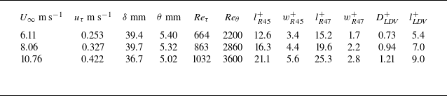
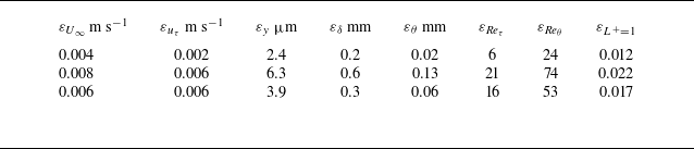


 u¯+
 σ(u′+)

 Reθ=3600

 Reθ=3600
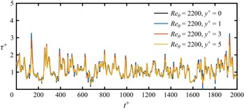
 Reθ=2200

 Reθ=3600
 Reθ=3600
 Reθ=2200

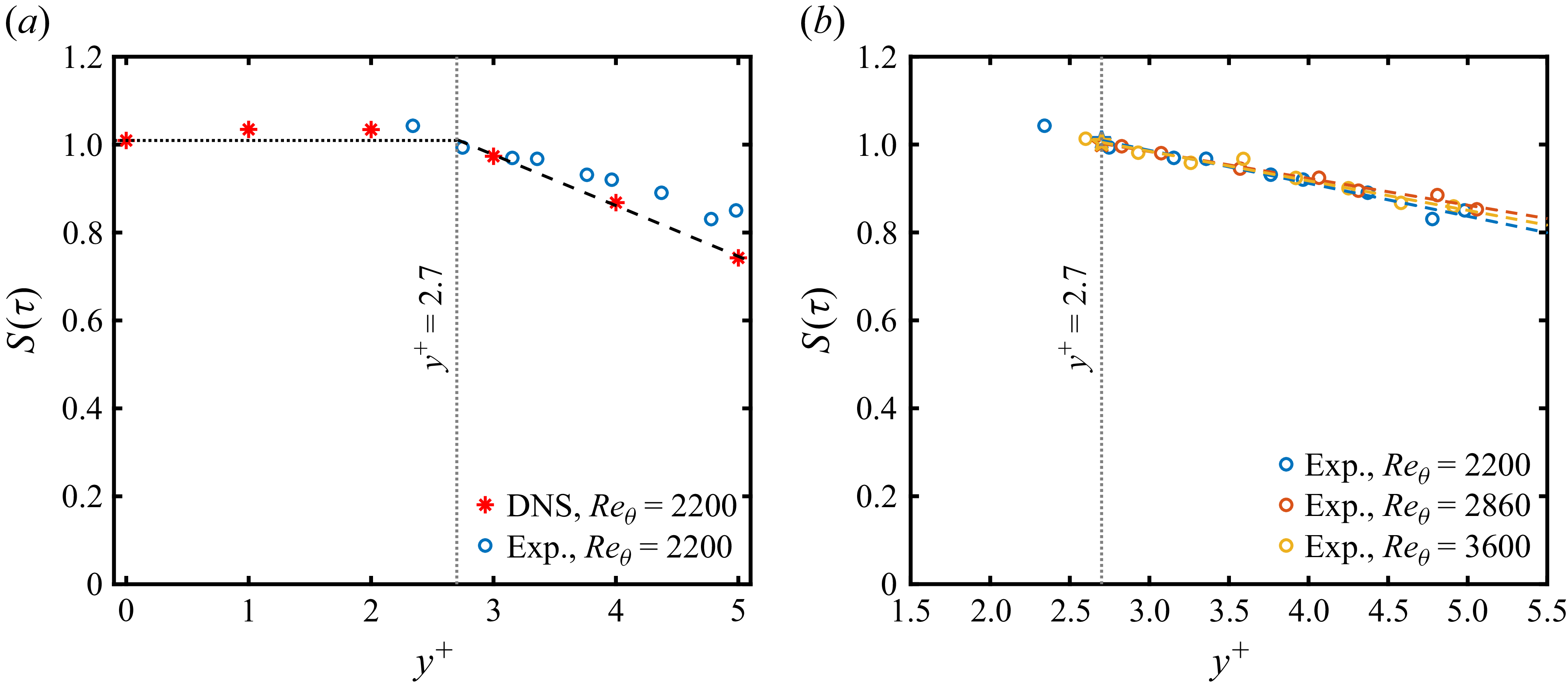
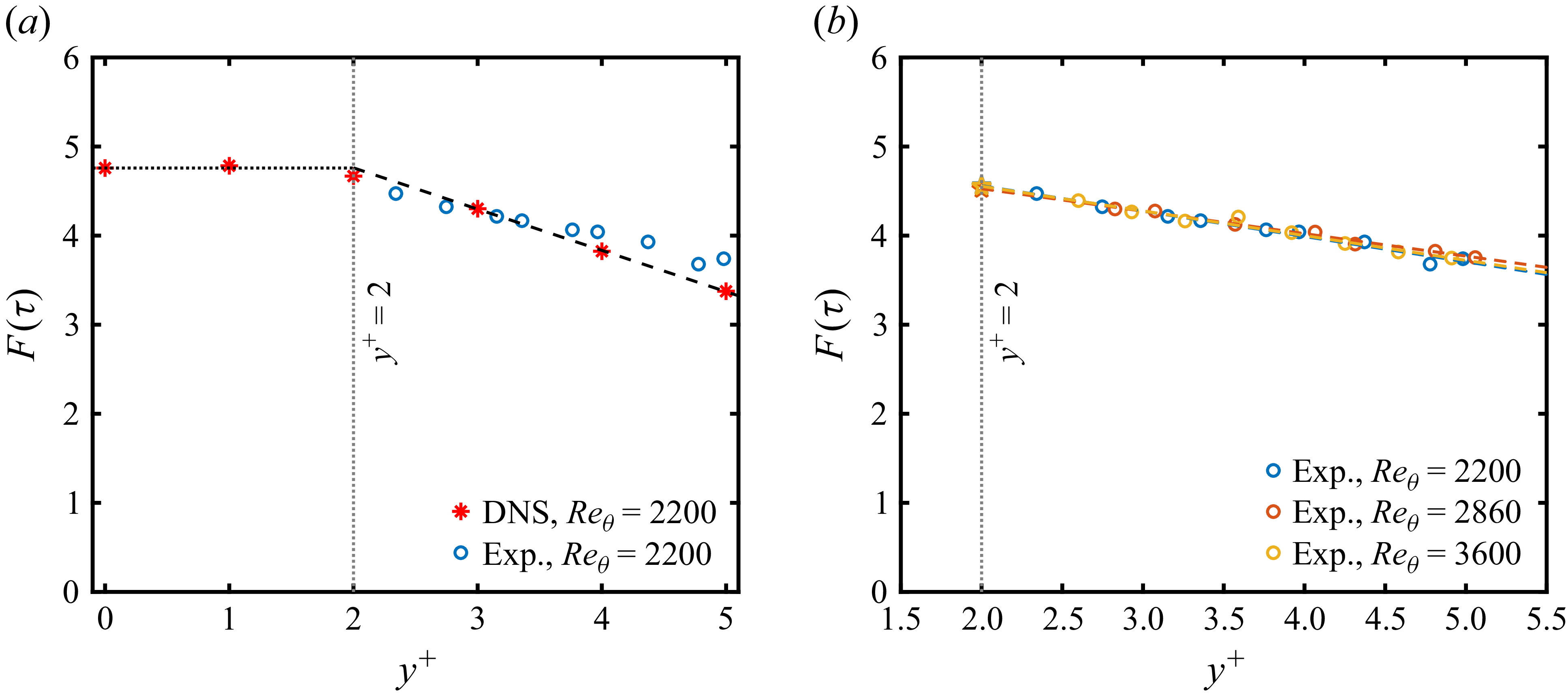

 Reθ=3600

 Reθ=2200
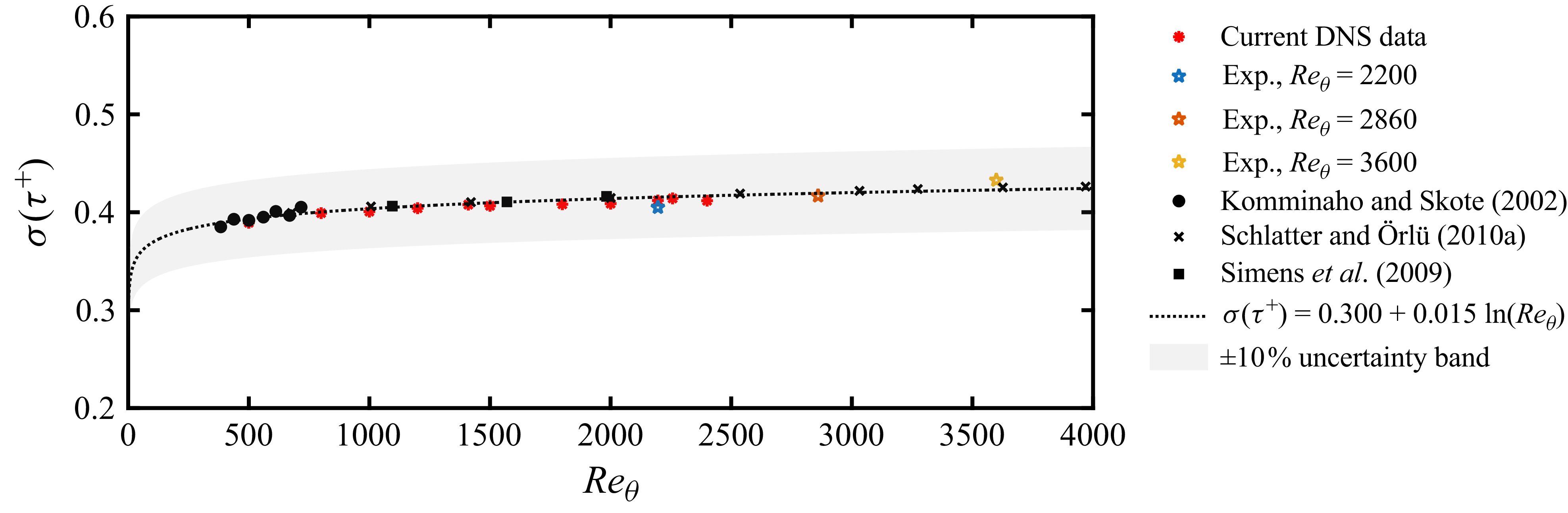
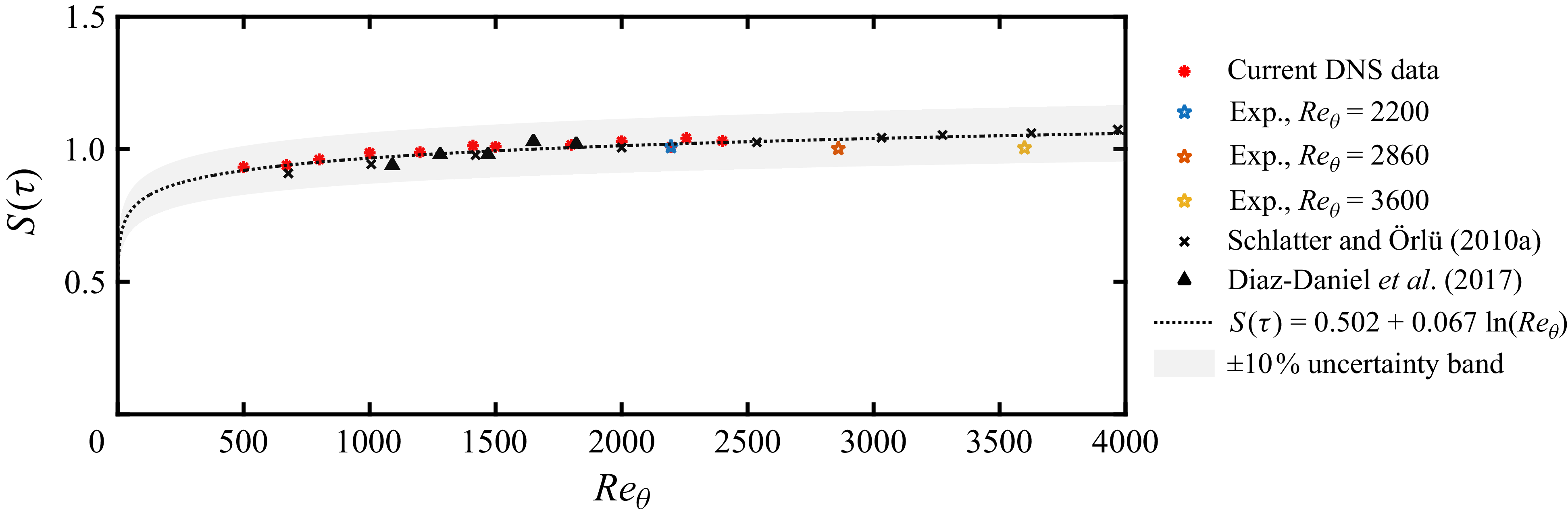
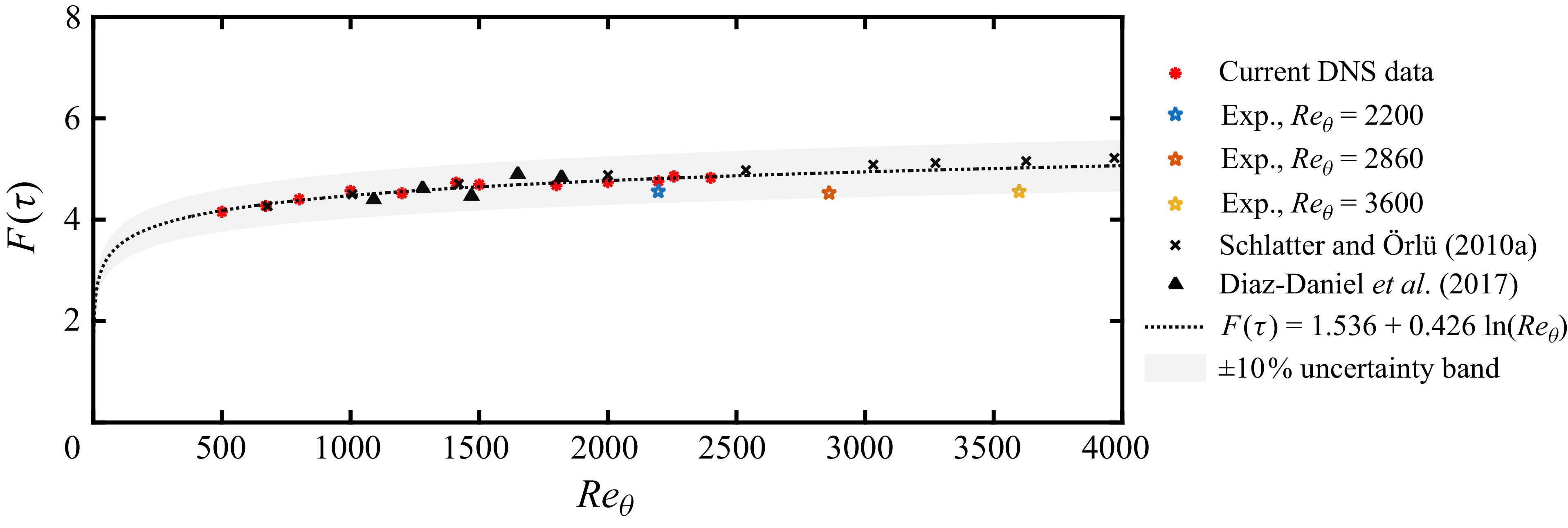
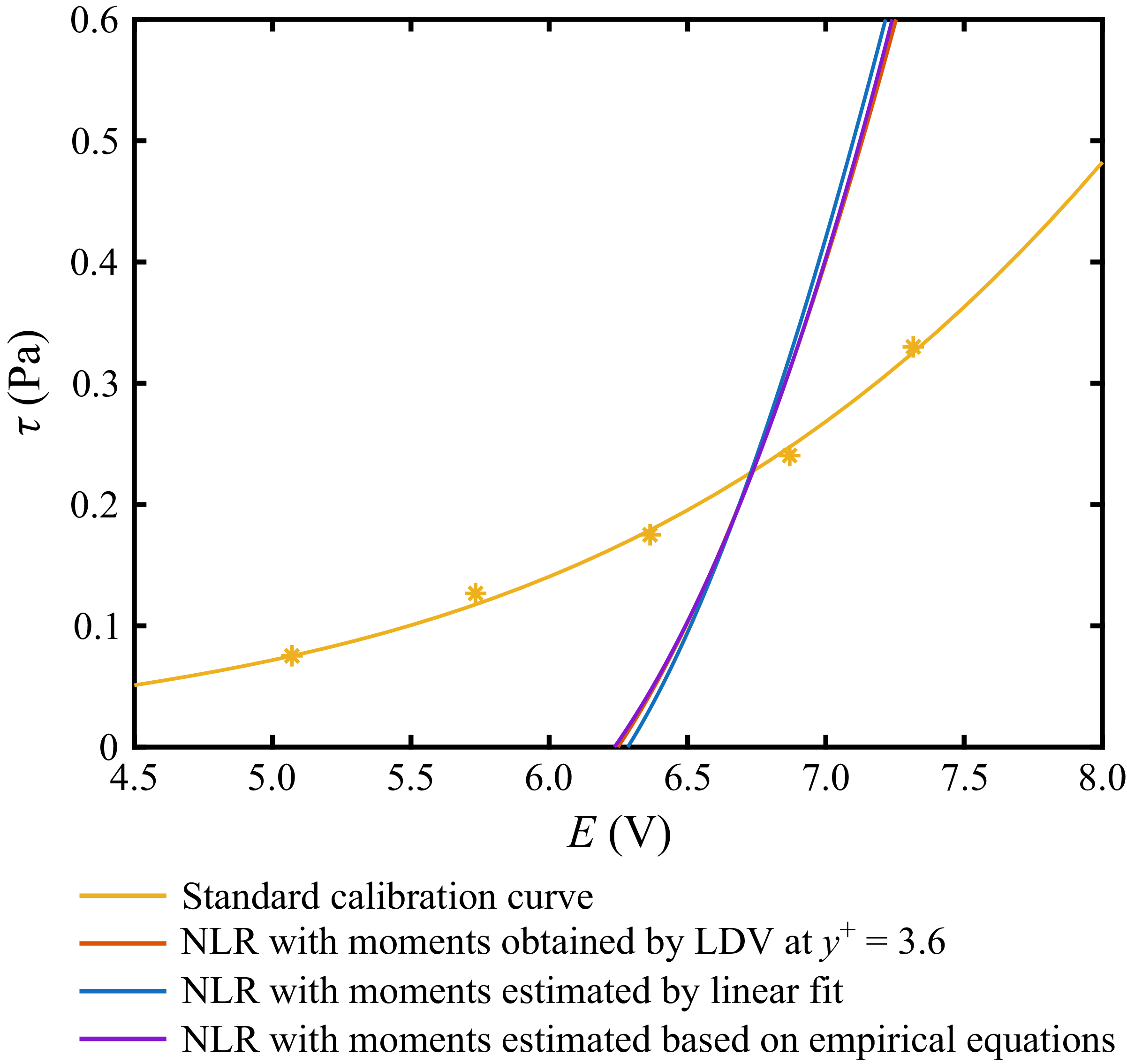
 Reθ=3600

 Reθ=3600

 Reθ=3600

 Reθ=3600

 T+>200
 T+>400
 T+>300
 T+>400

 y+=15
 T+>300
 T+>400


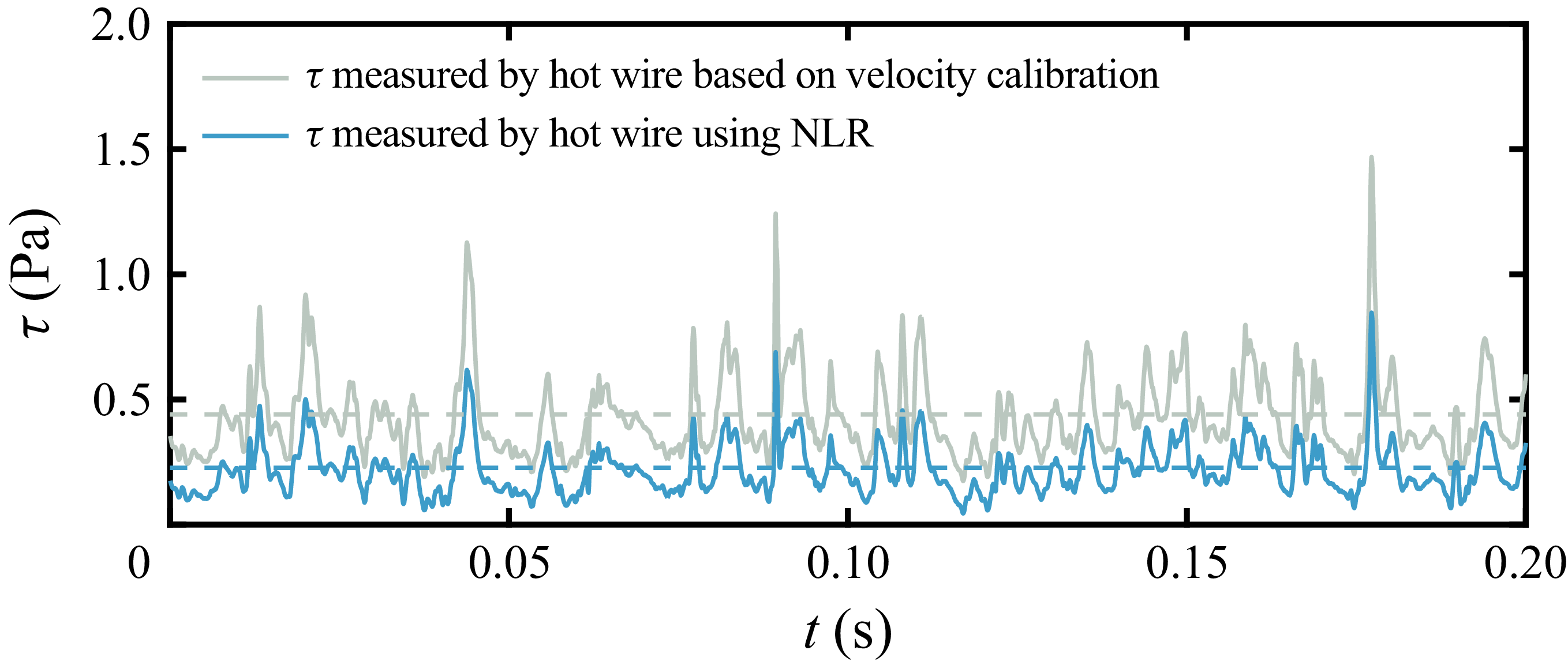


 y+=148
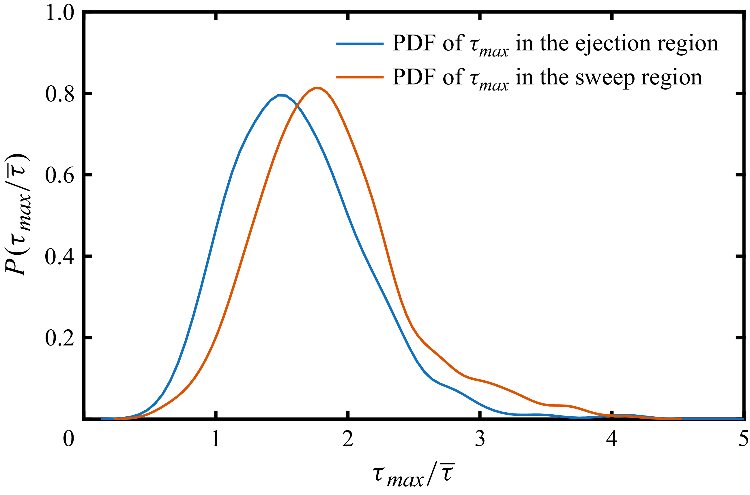


 Reθ=3600


 y+=0

 τ1
 τ2
 τr1
 τr2
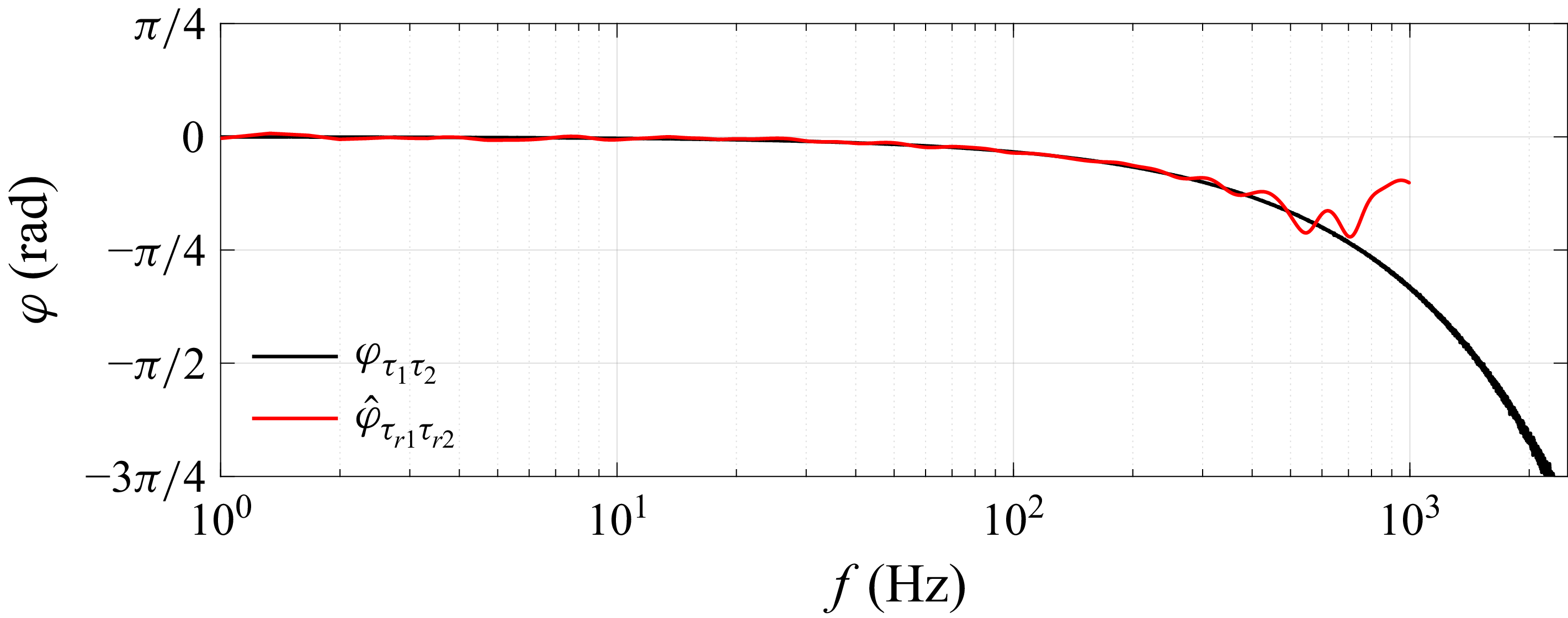


 Reθ=3600

 Open access

