Non-random measurement error, understood as mis-measurement of a variable that is systematically related to another variable, is a problem in many social science studies. For example, characteristics such as education affect whether survey respondents misrepresent their turnout behavior (Bernstein, Chandha and Montjoy Reference Bernstein, Chandha and Montjoy2001; Katz and Katz Reference Katz and Katz2010; Ansolabehere and Hersh Reference Ansolabehere and Hersh2012). The same is true for other sensitive questions, such as about corruption (Jensen, Li and Rahman Reference Jensen, Li and Rahman2010) or racial prejudice (Kuklinski, Cobb and Gilens Reference Kuklinski, Cobb and Gilens1997). Autocratic regimes have incentives to misreport official statistics like inflation or growth (Hollyer, Rosendorff and Vreeland Reference Hollyer, Rosendorff and Vreeland2011; Wallace Reference Wallace2016). Non-Governmental Organizations (NGOs) that provide data may over- or under-report some observations to further their advocacy role (Hill, Moore and Mukherjee Reference Hill, Moore and Mukherjee2013). Poor and less urbanized countries are more likely to miss infant deaths, leading to systematically biased infant mortality rates (Anthopolos and Becker Reference Anthopolos and Becker2009). The availability of cellphone coverage in an area may increase the probability that political violence is reported in event data (Dafoe and Lyall Reference Dafoe and Lyall2015; Weidmann Reference Weidmann2016). Historical data are more accurate for some areas than for others (Albouy Reference Albouy2012; Acemoglu, Johnson and Robinson Reference Acemoglu, Johnson and Robinson2012). And due to technological advances, time series data are more likely to miss relevant events further in the past, for example, war casualties or human rights abuses (Gohdes and Price Reference Gohdes and Price2013; Lacina and Gleditsch Reference Lacina and Gleditsch2013; Fariss Reference Fariss2014).
Best efforts notwithstanding, it is often impossible to eliminate such non-random measurement error or avoid data that contains it. This can lead to biased inference. In the cases cited above, debates about findings drawn from potentially problematic data have ensued, but they are the exception rather than the norm. The threat non-random measurement error poses to inference is not regularly addressed. Frequently, authors rely on informal arguments that the problem is not “bad enough” to render their inference invalid, or the issue is ignored (Herrera and Kapur Reference Herrera and Kapur2007). We argue that studies relying on potentially suspect data should take the threat this poses to inference seriously and routinely address it in a principled manner.
In this article, we aid researchers in this task by introducing a sensitivity analysis approach to non-random measurement error. It consists of three steps. First, researchers quantify the potential measurement error. While the true data-generating process is unobservable, a researcher tends to have an idea about what variable corrupts the data in what direction. We provide advice about how to quantify direction and magnitude of the potential non-random measurement error. In a second step, the variable is simulated given different assumptions about mis-measurement. Finally, these simulated variables are used to re-estimate the original model and the researcher can assess the inferential quantity of interest depending on the level of measurement error. To demonstrate the method, we apply it to two recent debates in the literature.
The simulation-based sensitivity analysis has a number of advantages for applied researchers. The method is simple to understand and execute, it can be used for any type of data or statistical model, and the results can be communicated in a straightforward manner. This makes it possible to routinely report how inference changes given different levels of measurement error, and to specify precisely how severe the error needs to be before the data no longer supports one’s hypotheses. It thus provides an important step toward increasing transparency in social science research.
The Problem of Non-Random Measurement Error
Why is There Non-Random Measurement Error?
In this paper, we are interested in measurement error that is systematically influenced by a second, “corrupting” variable. Why can observed data systematically differ from the truth? Two of the most common reasons are that there are differential incentives to misrepresent, or that the data creators systematically differ in their capabilities (Herrera and Kapur Reference Herrera and Kapur2007).
The problems posed by incentives are well known to survey researchers. Respondents often have reasons to answer questions untruthfully. The classic example is self-reported turnout, which is usually higher than actual election participation. This would not necessarily be problematic for inference if all non-voters were equally likely to misrepresent their behavior. However, there is evidence that characteristics such as education systematically influence over-reporting, leading to biased inference (e.g., Bernstein, Chandha and Montjoy Reference Bernstein, Chandha and Montjoy2001; Katz and Katz Reference Katz and Katz2010; Ansolabehere and Hersh Reference Ansolabehere and Hersh2012). The incentive problem in survey research is present for many other questions that address sensitive issues (e.g., Kuklinski, Cobb and Gilens Reference Kuklinski, Cobb and Gilens1997; Jensen, Li and Rahman Reference Jensen, Li and Rahman2010).
Incentive structures lead to inaccurate data outside of surveys as well. For example, national statistical agencies can be subject to political pressures. Autocratic regimes in particular tend to report information that overstates their performance (Hollyer, Rosendorff and Vreeland Reference Hollyer, Rosendorff and Vreeland2011; Wallace Reference Wallace2016). Many non-governmental organizations provide data, but their primary role is advocacy. These two can come into conflict. For example, the widely used torture data from Amnesty International overstates the severity of the problem when media coverage of the issue in a country is high (Hill, Moore and Mukherjee Reference Hill, Moore and Mukherjee2013).
A lack of capability is a second reason why true and reported data may diverge. Some countries have higher capabilities to accurately report information than others. Poor and less urbanized countries are more likely to miss relevant events, resulting in, for example, the systematic underestimation of their infant mortality rates (Anthopolos and Becker Reference Anthopolos and Becker2009). Historical data are often spotty, unevenly maintained, and not directly comparable (Albouy Reference Albouy2012). Increased data collection capabilities over time affect time series data, for example, on human rights abuses (Fariss Reference Fariss2014) or war casualties (Gohdes and Price Reference Gohdes and Price2013; Lacina and Gleditsch Reference Lacina and Gleditsch2013). And even with today’s modern technologies, measuring conflict is challenging. A recently popularized approach is to rely on data sets that measure conflict based on media coverage of violent events (e.g., Sundberg and Melander Reference Sundberg and Melander2013). But factors such as ruralness and cellphone coverage influence the probability that an incident is reported (Dafoe and Lyall Reference Dafoe and Lyall2015; Weidmann Reference Weidmann2016).
These are some examples showing that non-random measurement error is the subject of scholarly debates and that data quality is a concern in the social sciences. However, such systematic discussions are the exception rather than the norm (Herrera and Kapur Reference Herrera and Kapur2007). What are the consequences of ignoring the issue?
What are the Consequences of Non-Random Measurement Error?
Suppose we have n observations Y=(y 1, … , y n ), for which the following relationship is true:
 $$Y\,{\equals}\,\beta _{0} {\plus}\beta _{1} T{\plus}\beta _{2} C{\plus}\beta _{3} W{\plus}{\epsilon},$$
where T=(t
1, … , t
n
) is the treatment, C=(c
1, … , c
n
) and W=(w
1, … , w
n
) are two other variables, and ε=(ε
1, … , ε
n
) is a random error term such that ε
i
~N(0, σ
2). Denote the design matrix
Z
1
=[1, T, C, W]. If none of the variables contain measurement error, a standard Ordinary Least Squares (OLS) estimator
 $\left( {{\vskip 1pt{\hat {\beta }}} \,{\equals}\,\left( {{\bf Z}_{{\bf 1}} ^{T} {\bf Z}_{{\bf 1}} } \right)^{{{\!\minus}\!1}} {\bf Z}_{{\bf 1}} ^{T} Y} \right)$
will yield an unbiased estimate of
β
=[β
0, β
1, β
2, β
3].
However, suppose that instead of T we observe X=f(T|C). That is, the observed value is a function of the true value, conditional on the value of a “corrupting” variable. If we denote Z
2
=[1, X, C, W], we will obtain an OLS estimate
 ${{\hat{\delta }}} \,{\equals}\,\left( {{\bf Z}_{{\bf 2}} ^{T} {\bf Z}_{{\bf 2}} } \right)^{{{\!\minus}\!1}} {\bf Z}_{{\bf 2}} ^{T} Y$
. As we derive in the Online Appendix,
 ${{{\hat\delta }}} $
is a biased estimate of
β
, with the bias being
 $${\mib{\beta }} {\minus} {{\Bbb E}} ({{\hat{\delta }}} )\,{\equals}\,\left[ {\matrix{ {\beta _{1} \mathop{\sum}\limits_{i\,{\equals}\,1}^n {\left( {t_{i} {\minus}x_{i} } \right)\left( {d_{{11}} {\plus}d_{{12}} x_{i} {\plus}d_{{13}} c_{i} {\plus}d_{{14}} w_{i} } \right)} } \cr {\beta _{1} \mathop{\sum}\limits_{i\,{\equals}\,1}^n {\left( {t_{i} {\minus}x_{i} } \right)\left( {d_{{21}} {\plus}d_{{22}} x_{i} {\plus}d_{{23}} c_{i} {\plus}d_{{24}} w_{i} } \right)} } \cr {\beta _{1} \mathop{\sum}\limits_{i\,{\equals}\,1}^n {\left( {t_{i} {\minus}x_{i} } \right)\left( {d_{{31}} {\plus}d_{{32}} x_{i} {\plus}d_{{33}} c_{i} {\plus}d_{{34}} w_{i} } \right)} } \cr {\beta _{1} \mathop{\sum}\limits_{i\,{\equals}\,1}^n {\left( {t_{i} {\minus}x_{i} } \right)\left( {d_{{41}} {\plus}d_{{42}} x_{i} {\plus}d_{{43}} c_{i} {\plus}d_{{44}} w_{i} } \right)} } \cr } } \right],$$
where the terms denoted with d are the entries of a 4×4 matrix D ≡ (Z 2 T Z 2 )−1. Equation 2 provides a number of insights. First, bias depends on the sum of the differences between the true and the observed variable. Of course, this quantity is unobservable, so we cannot know the extent of the bias. Second, the systematic measurement error in X cannot only lead to bias in its associated coefficient but, depending on the covariance structure, it may also affect the coefficients of the other variables. Finally, note that the measurement error in X is caused by C, which is included in the regression. This means that simply controlling for the variable that induces mis-measurement may not be enough to obtain unbiased estimates.Footnote 1
To demonstrate the bias induced by non-random measurement error conditional on a corrupting variable, we conduct a Monte Carlo simulation. We simulate a variable Y with 1000 observations as in Equation 1, where
 $t_{i} \,\sim\,{\cal N}(3,\,2)$
,
 $c_{i} \,\sim\,{\cal B}(0.2)$
,
 $w_{i} \,\sim\,{\cal N}(1,\,1)$
, and
 ${\epsilon}_{i} \,\sim\,{\cal N}(0,\,1)$
. In addition, we allow for T and W to be correlated (at 0.3), which can happen in observational studies. Instead of T, we observe X where x
i
=ηt
i
whenever c
i
=1, with η=2. That is, for 20 percent of the observations, the observed value of the treatment is twice as high as the true value.
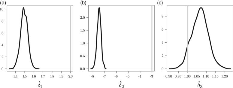
Figure 1 demonstrates that this leads to bias in all three coefficients of interest. Most importantly, the estimate of the treatment effect
 $\hat{\delta }_{1} $
is far away from the true value, as is the coefficient for the corrupting variable. If there is a correlation between T and the control variable W,
 ${\hskip -1pt \hat \delta }_{3} $
is also biased.Footnote
2
Thus, if a variable suffers from measurement error that is systematically determined by a “corrupting” variable, all estimated coefficients can be biased, resulting in misleading inference.
Monte Carlo simulation of the effect of non-random measurement error. (a) Coefficient  ; (b) Coefficient
 ; (c) Coefficient
 Note: Density of estimated coefficients with non-random measurement error. Gray lines show true coefficients.

What are Existing Approaches to Address the Problem?
One of the reasons for the lack of attention to non-random measurement error, we believe, is the sparsity of user-friendly statistical methods that can address the problem. There is a large literature on statistical approaches to address random measurement error, and a number of general and easy-to-use methods exist. Examples are simulation extrapolation, instrumental variable regression, or multiple overimputation (e.g., Carroll and Stefanski Reference Carroll and Stefanski1990; Cook and Stefanski Reference Cook and Stefanski1994; Guolo Reference Guolo2008; Blackwell, Honaker and King Reference Blackwell, Honaker and King2015). In comparison, the literature on non-random measurement error is relatively small.
One way to address non-random measurement error is to model it directly, for example, through regression calibration (for an overview see Carroll et al. Reference Carroll, Ruppert, Stefanski and Crainiceanu2006). The basic idea is to first find a model for E(T|X, Z), where Z is a covariate matrix. The main model is then estimated with E(T|X, Z) instead of the mis-measured variable X. While regression calibration is frequently used to address random measurement error, it is possible to incorporate non-random error as well (Kipnis et al. Reference Kipnis, Carroll, Freedman and Li1999, Reference Kipnis, Midthune, Freedman, Bingham, Schatzkin, Subar and Carroll2001). This approach requires a calibration data set that contains both T and X. With a few exceptions (e.g., election studies with validated turnout) such data are unfortunately not available to political scientists.
Another approach is to utilize statistical methods that account for the error in indirect ways, usually by adding a component that captures the “noise.” Hill, Moore and Mukherjee (Reference Hill, Moore and Mukherjee2013) accommodate an excess of “high torture” reports issued by Amnesty International by estimating a zero-inflated ordered probit model, where one equation focuses on the non-random measurement error. Anthopolos and Becker (Reference Anthopolos and Becker2009) introduce frontier regression, which splits the error term to include a one-sided term that captures the effect of non-random measurement error. However, both of these techniques are only applicable if the measurement error occurs in the dependent variable. They are also restricted with respect to the variable type they can accommodate.
A number of contributions instead develop variations of statistical estimators that are more robust to measurement error. Hug (Reference Hug2010) introduces a probit estimator developed by Hausman, Abrevaya and Scott-Morton (Reference Hausman, Abrevaya and Scott-Morton1998) that corrects for bias introduced by misclassification in the dependent variable. This is achieved through modeling the probability of misclassification explicitly. Betz (Reference Betz2013) develops a Two-Stage Least Squares (2SLS) instrumental variables estimator that is more robust to non-random measurement error in the endogenous variable. It makes use of the fact that rankings of observations are less sensitive to measurement error than the actual values. Again, both of these models require that the measurement error occurs in a specific type of variable, and are only applicable given certain research designs.
Finally, a different way to address non-random measurement error is sensitivity analysis. Its central idea is to test how violations of model assumptions affect inference. Sensitivity analysis has recently gained popularity in the context of (quasi-)experimental studies, where it is possible that unobserved confounders are correlated with treatment assignment and/or outcomes. The researcher identifies a range of scenarios where there are deviations from the ignorability assumption, and tests the sensitivity of the inference to those deviations (see Rosenbaum and Rubin Reference Rosenbaum and Rubin1983; Imbens Reference Imbens2003; Blackwell Reference Blackwell2014).
A small number of studies use the logic of sensitivity analysis to address non-random measurement error. The pioneering paper is Horowitz and Manski (Reference Horowitz and Manski1995), which analytically derives bounds on a population mean given systematic measurement error in the sampling procedure, using information on the maximum probability of data error. Both Imai and Yamamoto (Reference Imai and Yamamoto2010) and Kreider et al. (Reference Kreider, Pepper, Gundersen and Jolliffe2012) extend this approach to the estimation of bounds on the average treatment effect. Imai and Yamamoto (Reference Imai and Yamamoto2010) examine a situation in which there is misclassification in binary treatment assignment that is correlated with the outcome (differential measurement error). They formulate the problem as a constrained linear optimization, so assumptions are expressed as a linear equality plus inequality constraints. This is then used to solve for the sharp bounds of the Average Treatment Effect (ATE) using an algorithm for linear programming problems. Kreider et al. (Reference Kreider, Pepper, Gundersen and Jolliffe2012) analytically derive sharp bounds on the ATE of participation in a government program on various child health outcomes, given different assumptions on the magnitude and patterns of participation misreporting in household surveys. Finally, a Bayesian approach is taken by Tokdar et al. (Reference Tokdar, Grossmann, Kadane, Charest and Small2011), who develop a model of tropical cyclone activity over time that incorporates beliefs about the detection capability of different technologies as assumed priors.
Each of these studies develop a relatively complex model customized for a specific problem. In the next section, we generalize these different applications and introduce a general framework to use sensitivity analysis for non-random measurement error, that is mis-measurement of a variable systematically related to another variable.
Sensitivity Analysis for Non-Random Measurement Error
The sensitivity analysis approach to non-random measurement error asks: How would inference change if a variable suffered from non-random measurement error of various magnitudes? And how large would the error have to be to alter a study’s conclusions? The procedure consists of three steps, which we introduce in this section. A detailed guide that covers all types of variables can be found in the Online Appendix.
Step 1: Quantifying Measurement Error
Suppose we have n observations of a variable T=(t 1, … , t n ), which can be either a dependent or an independent variable. We suspect that T contains non-random measurement error driven by a “corrupting variable” C=(c 1, … , c n ). This means that instead of T, we observe X=(x 1, … x n )=f(T|C). The first step for the sensitivity analysis is to quantify the direction and potential magnitude of the error. That is, we model a “true” variable T′ as a function of X and C. How to specify T′ depends on the measurement level of both C and X. For simplicity, we begin with the case where C is binary.
Binary C
Assume we have reason to believe that an observed x i is accurate when c i =0, but that x i might be measured with error when c i =1. For these observations, we need to specify what the “true” T′ look like given the observed X and a certain level of error. The way to do this depends on whether X is binary, categorical, or continuous. Since the second option is a straightforward extension of the first (see Online Appendix), we focus here on the binary and continuous cases.
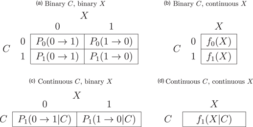
If X is binary, we specify a matrix of transition probabilities, as displayed in Panel (a) of Table 1. That is, for each combination of X and C, we specify the probability that if we observe a value of zero (one), the true observation is in fact one (zero). If we do not suspect any measurement error for c
i
=0, then P
0(0→1)=P
0(1→0)=0, so
 $t_{i}\!{\prime} \,{\equals}\,x_{i} $
in both cases. For c
i
=1, the transition probabilities depend on whether we believe there is systematic under- or over-reporting. If the concern is under-reporting, then P
1(1→0)=0 and P
1(0→1)=η. That is, observations for which c
i
=1 and x
i
=1 are assumed to be correctly reported. But when c
i
=1 and x
i
=0,
 $t_{i}\!{\prime} \,{\equals}\,1$
with probability η. If η is close to 0 the under-reporting is small. If η=1, then every single observation where c
i
=1 and x
i
=0 is misreported. If the concern is over-reporting, then P
1(0→1)=0 and P
1(1→0)=η.
Transition Probabilities and Transition Functions

If the corrupted variable X is continuous, we need to specify a transition function instead of a transition probability. This can be seen in Panel (b) of Table 1. Suppose again that we only suspect measurement error for c i =1. It follows that f 0(x i )=x i . For the set of observations where measurement error is suspected, we need to map the observed values X to the simulated “true” values T′ using a continuous function. One possibility is to model the “true” value as the observed value times a constant: f 1(x i )=ηx i . This means that the simulated true value is η times the value of x i . No measurement error is η=1. If η<1 then we suspect that the true values are lower than the reported one’s, and if η>1 we suspect that they are higher.
The idea of the sensitivity analysis is to simulate T′(η) for different values of η and see how the results of interest change. What range of η should be chosen? If the direction of the error is clear, one of the boundaries should correspond to no measurement error. The ideal scenario to determine the other boundary is that the researcher has auxiliary information on the magnitude of the measurement error. Even if conducted on different populations, such studies give ballpark measures about the maximum magnitude of the non-random measurement error. If no such “hard” data exists, advice from subject experts may be available, or the researcher may have priors about the degree of measurement error. To avoid confirmation bias, it is important that such priors are solicited before the sensitivity analysis is conducted. For example, a researcher could specify the transition probabilities or transition functions as well as the plausible magnitude of the error in a pre-registration plan. Finally, the boundary can be set arbitrarily high so the researcher can determine the value of η at which the substantive findings no longer hold.
The functional form of the transition function can be more complex than simply multiplying x i with a constant η. It might be useful to specify a step function where there is no measurement error for some values of X, but above a certain threshold error sets in. One could also use higher-order polynomials or logarithms.Footnote 3
Continuous C
There are occasions in the social sciences where the corrupting variable C is continuous. For example, measurement error may decrease (or increase) in Gross Domestic Product (GDP) per capita, the rate of urbanization, or time. If the corrupted variable X is binary, we again have to specify transition probabilities (see Panel (c) of Table 1). But instead of setting different probabilities for the different values of C, we now specify the transition probability as a continuous function of C. This could be a simple linear function, a logistic function, or variations thereof. The most complex case is the one where both the corrupting variable C and the corrupted variable X are continuous. While only one function needs to be specified (Panel (d) in Table 1), it needs to relate both C and X to T′ at the same time. For a more detailed discussion, see the Online Appendix.
Step 2: Simulation of Data
Having specified the transition probabilities or transition functions, the second step is to simulate what T′(η) looks like given different levels of measurement error. The basic idea is to take m equally spaced values for
 $\eta \in[\,\underline{\eta } ,\overline{\eta } ]$
and simulate T′(η).
Just like in the first step, how to simulate T′(η) and visualize how it compares to X depends on whether the variable is binary or continuous.Footnote 4 If X is binary we use transition probabilities, which makes it necessary to simulate the variable s times for each of the m values of η. If X is continuous, there is no need to simulate repeatedly.
In this step, it is important to gain a firm understanding of what T′(η) looks like for different values of η. We recommend carefully examining variable summaries and cross-tabulations as well as to plot the simulated observations against the observed ones, for example, using scatter plots or density functions. We provide detailed examples in the Online Appendix as well as our applications below.
Step 3: Model Re-Estimation With Simulated Data
The final step is to re-estimate the original model using the simulated T′(η) instead of the observed X for each of the m values of
 $\eta \in[\underline{\eta } ,\overline{\eta } ]$
. This provides the inferential quantity of interest, conditional on a given level of non-random measurement error.Footnote
5
The results can then be compared to the effect assuming no measurement error.
We recommend two ways to present the results of the sensitivity analysis. First, they can be summarized graphically by plotting the effect of interest over the entire simulated range of η. Second, a numerical summary can be given by determining the value of η at which the original finding can no longer be supported by the data (e.g., before it is no longer statistically different from 0 at a given confidence level). We denote this value by η*.
In many cases, η* is substantially meaningful and can easily be used to communicate the results of the sensitivity analysis. In other cases it is helpful to compare the mis-measured variable X to the simulated variable T′(η*) and report the value k* which solves the equation
 $${\Bbb E}\left( {T'\left( {\eta ^{{\asterisk}} } \right)} \right)\,{\equals}\,{\def {\tf="Macopen" E}}\left( X \right){\plus}k^{{\asterisk}} \sigma \left( X \right),$$
where σ stands for the standard deviation. The value of k* tells us how many standard deviations larger or smaller the mean of the true variable needs to be compared with the observed variable before the effect of interest is no longer supported by the data. This makes it possible to directly compare the sensitivity of different studies to systematic measurement error.
Limitations
Performing a sensitivity analysis to investigate the effects of potential non-random measurement error adds clarity and transparency to a study. But of course, this approach has some limitations that scholars should keep in mind. Most importantly, a sensitivity analysis cannot solve the problem of measurement error, since we do not know the exact relation between the true and the observed variable. If we did, we would simply use T instead of X. The goal of the sensitivity analysis is to specify plausible measurement error, and test the robustness of one’s inference to this error. If a small amount of error fundamentally changes the substantive inference the conclusion is clear, and the same is true if the results are robust to almost any realistic degree of error. But if η* falls in the middle of a range of plausible values, the case is more ambiguous. Sensitivity analysis will therefore be most useful if coupled with an analysis of the error in the data, when information from auxiliary sources is available, or when one has a strong set of beliefs about the measurement error. But even though a sensitivity analysis cannot bring certainty about what the results would be if the true data were available, it allows researchers to make informed quantitative statements about the limitations of their finding. This provides greater transparency to readers than informal assertions that the error is probably not “bad enough” to affect the findings significantly.
Second, a sensitivity analysis necessarily involves making assumptions about the magnitude and functional form of the measurement error. We usually have no way of testing them. However, the fact that we need to make strong assumptions to conduct a sensitivity analysis does not mean that not doing one is preferable. In fact, if we suspect that there is measurement error in the data, not conducting a sensitivity analysis makes the strongest (and most likely wrongest) assumption of all.
Application: Settler Mortality and Comparative Development
Having introduced the sensitivity analysis in a general way, we now apply it to two recent debates about the role of non-random measurement error on inference.Footnote 6 In our first application, we address potentially non-random measurement error in Acemoglu, Johnson and Robinson (Reference Acemoglu, Johnson and Robinson2001). That paper argues that less extractive institutions lead to higher economic development. Acemoglu, Johnson and Robinson (AJR henceforth) uses historic differences in European settler mortality as an instrument for institutional quality. Albouy (Reference Albouy2012) argues that the settler mortality data contains non-random measurement error that is severe enough to undermine the paper’s inference.
Because there is no single source for settler mortality rates, AJR combines data from different sources. The mortality data for most countries comes not from European settlers, but instead from European and American soldiers in the 19th century. For some countries these rates are taken from soldiers at peace in barracks, while others are taken from soldiers on campaign. This induces non-random measurement error because mortality rates for the latter are thought to be higher than for the former. Albouy finds that the results in AJR are not robust to removing the questionable data.
In their reply, Acemoglu, Johnson and Robinson (Reference Acemoglu, Johnson and Robinson2012) state that “there is no justification for discarding most of our data” and that “[s]imply throwing out data is certainly not a reasonable approach to deal with this wealth of information” (Acemoglu, Johnson and Robinson Reference Acemoglu, Johnson and Robinson2012, 3078). With respect to the soldier mortality rates, they argue that “there was little difference in practice” (Acemoglu, Johnson and Robinson Reference Acemoglu, Johnson and Robinson2012, 3079) between campaign and barracks rates. Both of these points motivate the kind of sensitivity analysis that we advocate for in this article. The data that suffer from measurement error can indeed still tell us something useful. However, we can do better than an informal statement that the problem is not “bad enough” to invalidate the findings.
Step 1: Quantifying Measurement Error
Not only is there suspicion that the mortality rates based on soldiers on campaign are overestimates, we also have information about the potential magnitude of the error. Citing Curtin (Reference Curtin1989), Albouy notes that mortality rates on campaigns were “66 to 2000 percent higher than barracks rates” (Reference Albouy2012, 3064–5). However, this crucial information is never used in further analysis. The simulation-based sensitivity analysis asks: What would the results look like given a certain degree of measurement error? In this example, do the results of AJR hold when the mortality rates for countries with campaign rates are 66 percent too high? 500 percent? 2000 percent?
Let x
i
be the observed mortality rate of country i, and let c
i
=1 if x
i
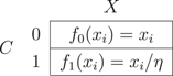
is a campaign rate. Table 2 shows the transition functions, where η∈[1, 21]. When η=1,
 $t_{i}\!{\prime} \,{\equals}\,x_{i} $
for all observations, so there is no measurement error. When η=21, the campaign rates are 21 times the barracks rate (2000 percent higher).
Transition Functions for Settler Mortality Rates X Depending on the Source of the Data C

Step 2: Simulation of Data
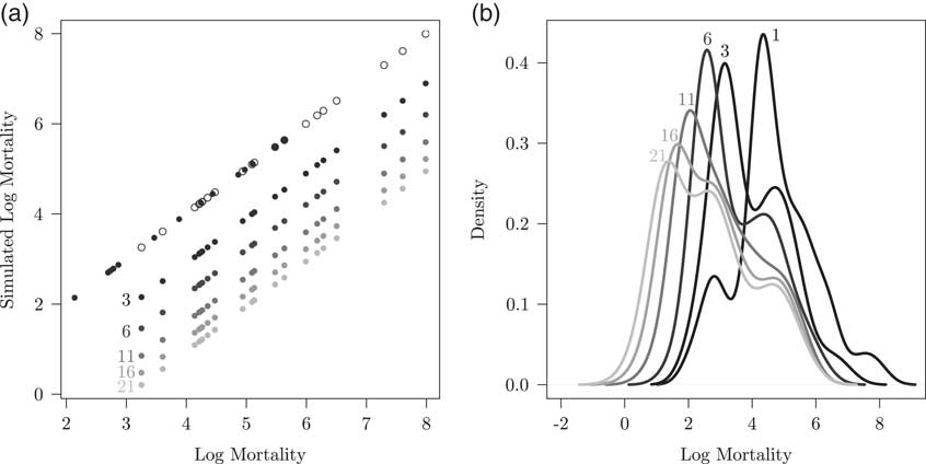
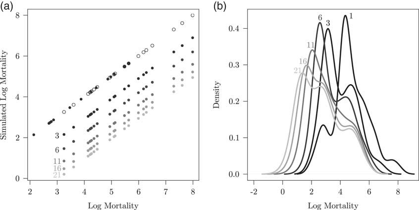
Given Table 2, we simulate what the variable would look like for η between 1 and 21. Figure 2 plots how this affects the data. Panel (a) shows the original log mortality data on the horizontal axis and log mortality given a certain value of η on the vertical axis. The black dots are cases that do not use campaign rates, and the open circles show those that do. The gray dots plot what the latter cases would look like for different values of η. Panel (b) plots what this implies for the densities of the log settler mortality variable.
Effect of η on log mortality rates Note: (a) Reported log mortality and “true” log mortality given η. Black dots: cases which do not use campaign rates. Open dots: cases which do use campaign rates. Gray dots: What cases using campaign rates would be for a given η. (b) Densities of original variable and those implied by different levels of η.
Step 3: Model Re-Estimation With Simulated Data
Finally, we re-estimate the model using our simulated variables with increasing amounts of error. The model is a 2SLS where the dependent variable is log GDP per capita in 1995 and the main independent variable is the quality of institutions, proxied by the average expropriation risk between 1985 and 1995. The latter is instrumented by the log settler mortality rates.Footnote 7
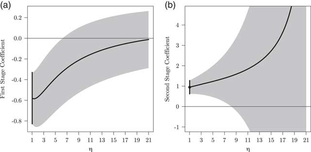
Figure 3 shows how the quantities of interest change conditional on the level of measurement error. Panel (a) plots the first-stage coefficient of log settler mortality (given η) on institutions. The relationship remains consistently and significantly negative unless the ratio of campaign rates to barracks rates is larger than about 6.2. If the non-random measurement error is greater than that, settler mortality no longer significantly predicts institutional quality, raising questions about its validity as an instrument.
Effect of η on first- and second-stage coefficient Note: (a) First Stage; (b) Second Stage. Point estimates with 95 percent confidence intervals. Black vertical lines: no measurement error.

Panel (b) shows the instrumented second-stage coefficient of institutions on economic development. It stays positive and distinct from 0 as long as the level of measurement error is less than a factor of η*=8.14. Beyond that, the standard error rapidly increases, reflecting the fact that settler mortality has become a weak instrument. The mean of the original log settler mortality variable is 4.657, with a standard deviation of 1.177. The mean of T′(η*) is 3.248. From Equation 3, it follows that k*=−1.197. That is, the measurement error must be severe enough so the average of the true variable is more than 1 standard deviation smaller than the one of the observed one.
This means the decision to combine campaign rates with barracks rates to obtain a measure of settler mortality does not necessarily invalidate the inference in AJR. If campaign rates are no more than eight times higher than barracks rates, the positive link between institutions and economic prosperity finds support in the data. However, given the auxiliary information on the severity of the measurement error, we cannot exclude the possibility that the results are driven by the usage of data that over-reports mortality for certain countries.
The sensitivity analysis thus moves the debate on this particular problem of non-random measurement error away from two polar extremes. On the one hand, Albouy (Reference Albouy2012) discards all data points that are potentially mis-measured. On the other hand, Acemoglu, Johnson and Robinson (Reference Acemoglu, Johnson and Robinson2012) maintain that the difference between campaign and barracks rates is too small to invalidate their results. Thanks to the sensitivity analysis, we now know just how large the difference needs to be before the original results no longer find support in the data.
Extensions
So far, we have deliberately focused on a simple setup of the sensitivity analysis: We assumed that we know exactly which observations were affected by the measurement error, we assumed that this error is equal for all of them, and we only looked at the effect of one corrupting variable. In this section, we show how each of these assumptions can be relaxed. The goal is not to provide an exhaustive list of extensions, or to demonstrate the one correct way to conduct them. Instead, we want to demonstrate the versatility of the sensitivity analysis approach.
Probabilistic subset affected by measurement error
The results above assume that every single country in which a rate taken from soldiers on campaign (c i =1) was used overstates the rate by a factor of η. But what if this is only true for a subset of observations? The flexible sensitivity analysis framework we propose can accommodate such a scenario by modifying the transition function in Table 2:
 $$\matrix{ {f_{1} (x_{i} )\,{\equals}\,r_{i} {{x_{i} } \over \eta }{\plus}(1{\minus}r_{i} )x_{i} } \cr {r_{i} \,\sim\,{\cal B}(\pi).}}$$
That is, a share π of the observations for which the rate was taken from soldiers on campaign are assumed to have measurement error, while the rest does not.
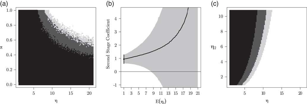
Panel (a) of Figure 4 plots the p-value of the second-stage coefficient of institutions conditional on the two parameters.Footnote 8 If π is low, the coefficient is significantly different from 0 for all values of η. The higher the share of observations affected, the lower the value of η at which the second-stage coefficient no longer reaches conventional levels of significance.
Results for three extensions Note: (a) p-value of the second-stage coefficient of institutions, conditional on the degree of measurement error η and the share π of observations with c i =1 affected. Black: p<0.01, dark gray: p<0.05, light gray: p<0.10, white: p>0.10. (b) Point estimates with 95 percent confidence intervals of second-stage coefficient of institutions with probabilistic η i . (c) p-value of the second-stage coefficient of institutions, conditional on the degree of measurement error in soldiers on campaign rate (η) and in bishops rate (η 2). Black: p<0.01, dark gray: p<0.05, light gray: p<0.10, white: p>0.10.

Probabilistic η
Another assumption we have made so far is that the degree of measurement error η is equal for all affected observations. The factor by which campaign rates are higher than barracks rates might be larger in some countries than in others. We modify the transition function in Table 2 as follows:
 $$\eqalignno{ f_{1} (x_{i} ) & \,{\equals}\,{{x_{i} } \mathord{\left/ {\vphantom {{x_{i} } {\eta _{i} }}} \right. \kern-\nulldelimiterspace} {\eta _{i} }} \cr \eta _{i} & \,{\equals}\,1{\plus}s_{i} \cr s_{i} & \sim{\rm Beta} \left( {\eta {\minus}1,\,\overline{\eta } {\minus}\eta } \right), $$
for
 $\eta \in[\,\underline{\eta } ,\overline{\eta } ]$
. This produces probabilistic draws of η
i
with the expected value being equal to η. Panel (b) of Figure 4 plots the point estimates and 95 percent confidence intervals of the second-stage coefficient, conditional on the expected value of η
i
.
Multiple corrupting variables
Finally, we have assumed that assigning some countries rates from soldiers on campaign and others from soldiers at peace is the only source of measurement error. What if there are multiple corrupting variables? Albouy (Reference Albouy2012) points to another issue in the data: rates for Latin American countries are taken from mortality rates of bishops. These are benchmarked to the mortality rate in Mexico (which is taken from French soldiers in campaign) by multiplying them by 4.25. However, “the ratio of actual soldier to bishop mortality rates varies from 0.98 to 10.80” (Albouy Reference Albouy2012, 3064). Because the benchmarking is done using rates from soldiers in campaign these two sources of mis-measurement are not independent, and the rates for Latin American countries suffer from two sources of error.
Let c i =1 if x i is a campaign rate and d i =1 if x i comes from bishops. The transition functions are as follows:
 $$\matrix{ {f_{1} (x_{i} )\,{\equals}\,x_{i} } & {{\rm if}\quad c_{i} \,{\equals}\,0\,{\rm and}\,d_{i} \,{\equals}\,0} \cr {f_{2} (x_{i} )\,{\equals}\,{{x_{i} } \over \eta }} & {{\rm if}\quad c_{i} \,{\equals}\,1\,{\rm and}\,d_{i} \,{\equals}\,0} \cr {f_{3} (x_{i} )\,{\equals}\,{{\eta _{2} } \over {4.25\;\eta }}x_{i} } & {{\rm if}\quad c_{i} \,{\equals}\,1\,{\rm and}\,d_{i} \,{\equals}\,1.}}$$
Note that a combination of c i =1 and d i =0 is not possible, since all rates that are benchmarked using the bishops data are affected by potential error in the soldiers data.
Panel (c) in Figure 4 shows the p-values of the second-stage coefficient conditional on the campaign/barracks rate and the benchmarking factor. There is an interactive effect between the two potential sources of non-random measurement error. If the way the bishop data are benchmarked in AJR leads to mortality rates that overstate the true level (η 2=0.98), the second-stage coefficient of institutions is not significant at the 5 percent level once the mortality of soldiers on campaigns is about four times higher than for those in barracks. If the benchmarking leads to mortality rates that understate the true level (η 2=11), the coefficient ceases to be significant at a campaign/barracks rate of about 11.
Application: Leadership and Democratic Deliberation
Our second application addresses the possibility of non-random measurement error in a binary variable. The study is a field experiment conducted by Humphreys, Masters and Sandbu (Reference Humphreys, Masters and Sandbu2006) in the Democratic Republic of São Tomé and Príncipe. In 2004, the government sponsored a series of meetings in which citizens met in small groups to discuss their priorities for economic policy. They were asked whether they prefer spending on medical clinics or hospitals, primary or secondary education, roads or public transportation, and so on. Each group was lead by a randomly assigned discussion leader and the discussion results on each policy choice recorded as a binary variable. The study finds that the policy preferences of the leaders significantly influence the discussion outcomes.
However, the leaders’ preferences were measured after the groups had completed their deliberations. The group outcome might thus have affected the leader’s stated preference. A leader could falsely report their policy preference as similar to the preference of the group to appear more effective, or because the discussion itself changed their mind. Alternatively, the leader might falsely report that they had the opposite of the group’s preference to be seen as fair and unbiased. The treatment assignment (leader opinion) therefore potentially suffers from measurement error that is directly correlated with the outcome variable. Using this example is particularly interesting since it allows us to compare our simulation-based framework with the analytical sensitivity analysis proposed by Imai and Yamamoto (Reference Imai and Yamamoto2010). They show that the Average Treatment Effect (ATE) includes 0 when the maximum probability of misclassification exceeds between close to 0 and about 25 percent, depending on the question.
Denote the outcome of group discussion i on a certain policy with y i ∈{0, 1}. Note that in this application, the dependent variable is the corrupting factor, so we use Y instead of C. The stated policy preference of the leader is x i ∈{0, 1}. As discussed above, the direction of the measurement error is not clear here. There are plausible reasons for discussion leaders to misreport their policy preferences so they align with or diverge from the group outcome. We therefore examine the two extreme scenarios.Footnote 9
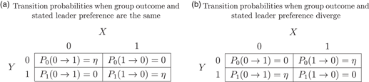
Panel (a) in Table 3 shows the transition probabilities for the scenario in which there is no measurement error when the group outcome and the stated leader preference diverge. When they are the same, the stated answer may not accurately reflect the pre-treatment preference with probability η. In the second scenario, shown in Panel (b), we assume that there is no measurement error when the group outcome and the stated leader preference are the same, but that there is measurement error with probability η when they diverge.
Transition Probabilities for Stated Leader Preference X and Group Discussion Outcome Y

We follow Imai and Yamamoto (Reference Imai and Yamamoto2010) and evaluate the entire range η∈[0,1]. We simulate 500 draws for each value of η and take the median coefficient and standard error of the draws, which we then use to compute the ATE. The focus here is on one outcome of the group discussions: Whether money should be invested in clinics (y i =0) or hospitals (y i =1). A discussion of other questions can be found in the Online Appendix.
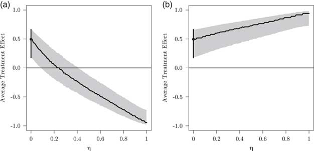
Figure 5 shows the results. Panel (a) is the first scenario, where we assume that some leaders who report that their personal preference matches the group outcome are misclassified. Assuming no measurement error, the ATE is around 0.5. However, the ATE decreases if it is the case that some leaders stated that their preference matched the group outcome when in fact it did not. The ATE is no longer positive and statistically different from 0 for η* of around 0.1, so when 10 percent of leaders are misclassified. Once more than around 40 percent misstate their preference, the ATE is negative.
Effect of η on the average treatment effect Note: (a) Scenario (a) from Table 3; (b) Scenario (b) from Table 3. Point estimates with 95 percent confidence intervals. Black vertical lines: no measurement error.

Panel (b) plots the scenario where we assume that some leaders who report that their personal preference does not match the group outcome are misclassified. If this is the case, there are in truth more leaders whose preference is the same as the group outcome. A naive estimate that assumes no measurement error thus underestimates the ATE. The higher the share of misclassified observations, the larger the effect of discussion leaders on the outcome.
How does our simulation-based sensitivity analysis compare with the analytical one proposed by Imai and Yamamoto (Reference Imai and Yamamoto2010)? In their approach, Imai and Yamamoto formulate the problem as a constrained linear optimization, so assumptions need to be expressed as a linear equality and inequality constraints. This is then used to solve for the sharp bounds of the ATE using an algorithm for linear programming problems.
The main difference between the two approaches in how the problem is set up is that we express the potential measurement error as T′=Pr(X|Y, η), and their approach amounts to specifying X=Pr(T′|Y, ρ). While we quantify the true data conditional on the observed data, they express the observed data conditional on the truth. However, the substantive insights of both approaches are very similar.
The main difference in terms of execution is that Imai and Yamamoto are able to solve for explicit analytical solutions of the large sample bounds. Because our approach relies on simulations, it can only approximate solutions.Footnote 10 At the same time, it places a lower burden on applied researchers. Instead of having to formulate the problem in the form of a constrained linear optimization, they only need to specify a simple equation relating C to X. Once the variable T′ for different values of η has been simulated, the effect of non-random measurement error can be assessed by simply re-running the original statistical model. This makes it possible for researchers to routinely check the sensitivity of any of their results if they suspect that non-random measurement error is present.
Conclusion
One of the most important prerequisites for valid scientific inference is accurate data. Unfortunately, this is often more difficult in the social sciences than in other disciplines. We frequently have to rely on primary data collected for other purposes and by people who may have incentives to not report everything accurately. Some measures we are interested in are so difficult to quantify that some observations will be systematically more accurate than others. And even if we can collect our own primary data, factors such as social desirability bias, fear of repercussions, or research budget constraints may still be at work. That is to say, non-random measurement error is a part of many political scientists’ life, no matter their subfield or their preferred type of data.
This does not mean that we should not conduct studies using such data, as it still can provide us with important information. At the same time, the bias introduced by non-random measurement error cannot be ignored either. In this article, we have argued that the threat to inference it poses should be addressed routinely. To aid researchers in doing so, we have presented a simulation-based procedure that checks the sensitivity of results to different levels of non-random measurement error. The major advantages of the sensitivity analysis approach are that it can be used for any kind of data, variable, and statistical model, that it does not require additional data typically not available in the social sciences, and that it is comparatively simple to implement and communicate. This allows researchers to routinely use it in their work.
In recent years, political science research has undergone a remarkable transformation. Studies now use sophisticated methodological techniques, and the identification revolution has brought a focus on careful research design. Similarly, it is less and less acceptable to only present a few select model specifications. Researchers now check the robustness of their inference using different statistical estimators and various combinations of control variables and data subsamples. They also employ alternative measures, account for missing data, and examine the sensitivity to omitted variables. We believe that addressing measurement error is the next logical step in this trajectory toward increased transparency and the provision of better safeguards against “false positive” findings. Our hope is that this article inspires researchers to think about potential non-random measurement error in their data, and about how it may affect their inference. We also provide the conceptual framework and the methodological tools to address the problem in a principled manner.