2 Hamiltonian description of the beam–plasma interaction

The BPS describes the nonlinear dynamics of a fast electron beam interacting with a background plasma in a one-dimensional approximation. The dynamics is regulated by the Vlasov–Poisson equation, when collisions can be neglected (i.e. the collision frequency is much smaller than the plasma frequency). Such a system describes the coupled dynamics of the electric field and the electron distribution function and its analytical treatment is limited by the nonlinear character of the resulting dynamics. For a description in terms of a graph theory, see Al'Tshul & Karpman (Reference Al'Tshul and Karpman1966). However, when addressing the numerical study of the Vlasov–Poisson system, a significant simplification is offered by the Hamiltonian approach (O'Neil et al. Reference O'Neil, Winfrey and Malmberg1971; Elskens & Escande Reference Elskens and Escande2003). In this representation, the electron distribution function is reduced to a discrete set of beams (actually, on a numerical level, such an issue is conceptually mandatory) and then the self-consistent evolution of Newton's second law for the electrons and of the Fourier-transformed Poisson equation for the electric field (generated by the charge displacement) is naturally addressed in terms of dimensionless universal quantities. From a numerical point of view, this approach is less demanding with respect to the direct integration of the Vlasov equation. As a result, a large number of resonances can be easily described, up to dealing with the so-called quasi-linear limit (Berk et al. Reference Berk, Breizman, Fitzpatrick and Wong1995a; Volokitin & Krafft Reference Volokitin and Krafft2012). The conceptual framework that justifies the implementation of a Hamiltonian approach is the so-called notion of ‘quasi-stationary states’ (Berk et al. Reference Berk, Breizman and Pekker1995b; Elskens & Escande Reference Elskens and Escande2003; Carlevaro et al. Reference Carlevaro, Fanelli, Garbet, Ghendrih, Montani and Pettini2014), i.e. transient states of the discrete system, in which a time is spent by the dynamics proportional to the number of considered particles (in practice, charged macroparticles). Such states approach for a diverging number of particles, i.e. in the continuum limit, the equilibrium configuration of the Vlasov–Poisson system.

In this work, following O'Neil & Malmberg (Reference O'Neil and Malmberg1968) and O'Neil et al. (Reference O'Neil, Winfrey and Malmberg1971) (see also Carlevaro et al. (Reference Carlevaro, Falessi, Montani and Zonca2015, Reference Carlevaro, Milovanov, Falessi, Montani, Terzani and Zonca2016a) for other reference details), the plasma is addressed as a cold linear dielectric medium represented by longitudinal electrostatic Langmuir waves, whose density $n_{\textrm {p}}$ is assumed much greater that the beam density $n_{\textrm {B}}$. In this respect, we define $\eta \equiv n_{\textrm {B}}/n_{\textrm {p}}$ as one of the fundamental parameters of the model. The Langmuir wave is described in terms of the corresponding modes whose frequencies $\omega$ are very close to the plasma frequency $\omega _{\textrm {p}}$: the dielectric function (for a fixed mode) 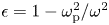$\epsilon =1-\omega _{\textrm {p}}^2/\omega ^2$ is, thus, nearly vanishing. This allows one to write an evolutive equation for the modes corresponding to the Poisson equation. The simple force equation governs, instead, the particle dynamics. A single mode is set to be resonantly excited by the beam, considering wavenumber $k=\omega /v_{\textrm {r}}$, where $v_{\textrm {r}}$ is a fixed initial resonant velocity of the beam particles.

In this scheme, the cold background plasma is considered as a periodic slab of length $L$, and particle positions are labelled by $x_i$ ($i=1,\ldots ,N$, where $N$ indicates the total particle number). The Langmuir wave scalar potential $\varphi (x,t)$ is addressed by means of the Fourier components $\varphi _k(t)$ and we use the following dimensionless quantities: $\bar {x}_i=x_i(2{\rm \pi} /L)$, $\tau =t\omega _{\textrm {p}}$, $u_i=\bar {x}_i'=v_i(2{\rm \pi} /L)/\omega _{\textrm {p}}$, 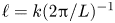$\ell =k(2{\rm \pi} /L)^{-1}$, $\phi _\ell =(2{\rm \pi} /L)^2 e\varphi _\ell /m\omega _{\textrm {p}}^2$, $\bar {\phi }_\ell =\phi _\ell \textrm {e}^{-\textrm {i}\tau }$. The derivative with respect $\tau$ is indicated with the prime, while barred frequencies (and the related growth rates) are normalized as $\bar {\omega }=\omega /\omega _{\textrm {p}}$ ($\bar {\gamma }=\gamma /\omega _{\textrm {p}}$). The governing equations of the BPS read

(2.1)\begin{equation} \left. \begin{aligned} \bar{x}_i' & =u_i,\\ u_i' & =\sum_{\ell}\left(\textrm{i}\,\ell\;\bar{\phi}_\ell\;\textrm{e}^{\textrm{i}\ell\bar{x}_{i}}+\textrm{c.c.}\right),\\ \bar{\phi}_\ell' & =-\textrm{i}\bar{\phi}_\ell+\frac{\textrm{i}\eta}{2\ell^2 N}\sum_{\ell} \textrm{e}^{-\textrm{i}\ell\bar{x}_{i}}, \end{aligned} \right\} \end{equation}

while the resonance condition is $\ell =\bar {\omega }/u_{\textrm {r}}$.

As reference case for the analysis of this work, we consider a positive slope as initial warm beam distribution function in the velocity space:

(2.2)\begin{equation} F_0(u)=0.5\;\text{Erfc}[a-b\,u], \end{equation}

with the beam distributed from $u_{\min }=0.001$ to $u_{\max }=0.002$ (with $a\simeq 6.8$ and $b\simeq 4537$). In the nonlinear simulations, we initialize $N=10^{6}$ particles and implement a Runge–Kutta (fourth-order) algorithm to solve (2.1). Actually, the initialization in the velocity space is formal and particles are free to spread in this coordinate, while we consider uniform initial conditions for the particle positions between $0$ and $2{\rm \pi}$ and we apply periodic boundary conditions in this range for $\bar {x}_i$. Specifically, we discretize the beam profile in 500 delta-like beams, each of them having a single fixed velocity. Each beam is also initialized with random generated positions and with a number of particles provided by (2.2) (normalized to $N$). This procedure provides the initial $2\times N$ array for $(\bar {x}_i,u_i)$ which is evolved in time self-consistently with the modes. The particles are thus considered as points in the phase space and no $(\bar {x},u)$-meshes are required. The modes are instead initialized at $\textit{O}(10^{-14})$ (this guarantees the initial linear regime). For the considered time scales, both the total energy and momentum (for the explicit expressions, see Carlevaro et al. (Reference Carlevaro, Falessi, Montani and Zonca2015)) are conserved with relative fluctuations of approximately $1.4\times 10^{-5}$.

We conclude by writing down the the linear dispersion relation for electric field perturbations. Using dimensionless variables, it reads (O'Neil & Malmberg Reference O'Neil and Malmberg1968; Lifshitz & Pitaevskii Reference Lifshitz and Pitaevskii1976)

(2.3)\begin{equation} 2(\bar{\omega}_0+\textrm{i}\bar{\gamma}_{\textrm{L}}-1)-\frac{\eta}{\ell M} \int_{-\infty}^{+\infty}\,\textrm{d}u\frac{\partial_u F_0(u)}{u\ell-\bar{\omega}_0-\textrm{i}\bar{\gamma}_{\textrm{L}}}=0, \end{equation}

where $M=\int F_0(u)\,\textrm {d}u$ and we have explicitly written $\bar {\omega }=\bar {\omega }_0+\textrm {i}\bar {\gamma }_{\textrm {L}}$. Here, $\bar {\omega }_0$ includes a small real frequency shift with respect to $\omega _{\textrm {p}}$ and $\bar {\gamma }_{\textrm {L}}$ indicates the normalized linear growth rate (Carlevaro, Montani & Zonca Reference Carlevaro, Montani and Zonca2018). This expression describes the inverse Landau damping mechanism, and defines the linear instability condition of a single mode through the resonance pole $u=\bar {\omega }_0/\ell$.

2.1 Nonlinear velocity spread

Let us now review some basic nonlinear features of the BPS in the single-mode assumption, by means of numerical simulations of (2.1). The dynamics of one isolated unstable mode consists of an initial exponential growth (characterized by $\bar {\gamma }_{\textrm {L}}$) followed by nonlinear saturation, where particles are trapped and begin to slosh back and forth in the potential well of the wave. This makes the mode intensity oscillate and generates rotating clumps in the phase space. In Berk et al. (Reference Berk, Breizman and Pekker1995b) (and references therein), also verified was the existence of two distinct saturation regimes in the presence of source and sink. They correspond, on the one hand, to the previously discussed steady-state saturation and, on the other hand, to the so-called pulsating scenario corresponding to large mode damping rate (not addressed in the present paper).

A quadratic relation exists (Fried et al. Reference Fried, Liu, Means and Sagdeev1971; O'Neil et al. Reference O'Neil, Winfrey and Malmberg1971; Levin et al. Reference Levin, Lyubarski, Onishchenko, Shapiro and Shevchenko1972) between the saturation level of the considered linearly unstable mode (dubbed $|\bar {\phi }|^{S}$) and the linear growth rate, i.e. $|\bar {\phi }|^{S}=\alpha \bar {\gamma }_{\textrm {L}}^{2}$ (with $\alpha =\textrm {const.}$). This relation holds only if the nonlinear dynamics is not sensitive to the morphology of the distribution function (Carlevaro et al. Reference Carlevaro, Montani, Wang and Zonca2016b; Chen & Zonca Reference Chen and Zonca2016); and all the studies reported in the present work satisfy this condition.

Assuming a single-mode scheme, the approximation of the post-saturation dynamics by an instantaneous harmonic oscillator allows one to identify the so-called trapping (bounce) frequency $\omega _{\textrm {B}}$ as

(2.4)\begin{equation} \bar{\omega}_{\textrm{B}}=\sqrt{2\ell^{2}|\bar{\phi}|^{S}}= \sqrt{2\alpha}\;\ell\,\bar{\gamma}_{\textrm{L}}. \end{equation}

Meanwhile, from energy conservation at saturation, one can estimate the nonlinear velocity spread of resonant particles, i.e. particles having velocity $u_{\textrm {r}}=1/\ell$ (here and in the following, we approximate $\bar {\omega }_0=1$). This quantity is clearly related to the (half) rotating clump width mentioned above and it is derived from the relation $m(\Delta \tilde {v}_{\textrm {NL}})^{2}/2=e|\varphi (x,t)|^{S}$. Using dimensionless variables, this definition of the nonlinear velocity spread can be cast as

(2.5)\begin{equation} \Delta\tilde{u}_{\textrm{NL}}/u_{\textrm{r}}=2\ell\sqrt{|\bar{\phi}|^{S}}= \sqrt{2}\,\bar{\omega}_{\textrm{B}}=2\ell\sqrt{\alpha}\;\bar{\gamma}_{\textrm{L}}. \end{equation}

This estimate does not account for effects of non-resonant particles. Thus, in order to get a satisfactory characterization of the nonlinear dynamics, we introduce the clump width $\Delta {u}^{c}_{\textrm {NL}}$ defined by measuring the maximum instantaneous velocity of particles initialized at $\tau =0$ with $u < u_{\textrm {r}}$; and, similarly, the minimum velocity of particles initialized with $u>u_{\textrm {r}}$. This corresponds to monitoring the instantaneous spread of particles above and below resonance. Such a measure is performed during the temporal evolution of the system and $\Delta {u}^{c}_{\textrm {NL}}$ is taken as the value at saturation time $\tau _{\textrm {S}}$.

Let us discuss the behaviour of the quantities introduced above, as a function of the linear growth rate. The following analysis refines well-known results reported in the literature, mainly derived for linear shapes of the initial distribution profile (Fried et al. Reference Fried, Liu, Means and Sagdeev1971; O'Neil et al. Reference O'Neil, Winfrey and Malmberg1971; Levin et al. Reference Levin, Lyubarski, Onishchenko, Shapiro and Shevchenko1972; Wu et al. Reference Wu, White, Chen and Rosenbluth1995, Reference Wu, Cheng and White1994), enlightening the crucial role of wave–particle trapping for nonlinear mode saturation and resonance broadening. We study five distinct cases having different resonant velocities (namely $u_{\textrm {r}}\simeq 0.0013,\ 0.0014,\ 0.0015,\ 0.0016,\ 0.0017$). For each case, 10 simulations with different $\eta$ values are studied (equispacing the $\eta$ value from $0.00015$ to $0.0025$), providing distinct drives $\bar {\gamma }_{\textrm {L}}$ by means of (2.3), and then linear fits are implemented to estimate the scalings. We obtain the following behaviours:

(2.6)\begin{gather} |\bar{\phi}|^{S}=1.27\pm0.38\times10^{-5}\;\bar{\gamma}_{\textrm{L}}^{2}, \end{gather}

(2.7)\begin{gather} \bar{\omega}_{\textrm{B}}=3.31\pm0.07\;\bar{\gamma}_{\textrm{L}}, \end{gather}

(2.8)\begin{gather} \Delta\tilde{u}_{\textrm{NL}}/u_{\textrm{r}}=4.72\pm0.1\;\bar{\gamma}_{\textrm{L}}, \end{gather}

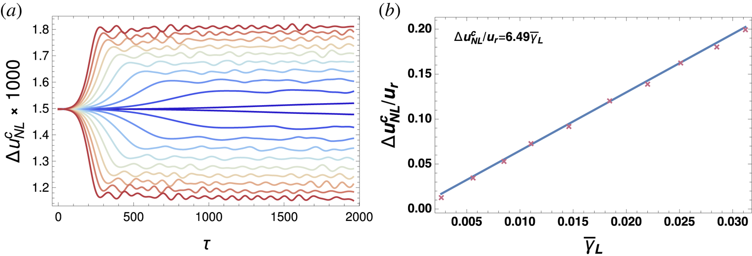
(2.9)\begin{gather} \Delta u^{c}_{\textrm{NL}}/u_{\textrm{r}}=6.64\pm0.15\;\bar{\gamma}_{\textrm{L}}. \end{gather}

Regarding the measured clump width, for the sake of completeness, we show the details of the case at the inflection point of $F_0$ ($u_{\textrm {r}}\simeq 0.0015$). In figure 1(a), we plot the clump width $\Delta {u}^{c}_{\textrm {NL}}$ versus time and for the different values of $\eta$ (different colours in the figure): as expected, the smaller the value of $\eta$, the smaller is $\Delta {u}^{c}_{\textrm {NL}}$. In fact, as the value of $\eta$ is lowered, the instability drive becomes correspondingly weaker, and, in turn, the electric field amplitude at saturation and the clump width are decreased. We observe that, for a fixed $\eta$ value, the clump width increases with time during the linear instability growth phase, until the saturation level is reached. In figure 1(b), we instead illustrate the behaviours of $\Delta {u}^{c}_{\textrm {NL}}$ as a function of the linear drive outlining the linear scaling.

Figure 1.

Case $u_{\textrm {r}}\simeq 0.0015$: crosses represent simulation results while solid lines are linear fits. (a) Plot of the clump width $\Delta {u}^{c}_{\textrm {NL}}$ as a function of $\tau$. Different colours represent the 10 equispaced values of $\eta \in [0.00015\,(\text {blue}),\ 0.0025\,(\text {red})]$. (b) Dependence of $\Delta {u}^{c}_{\textrm {NL}}$ as a function of $\bar {\gamma }_{\textrm {L}}$.

We emphasize that repeating the analysis above with different slope of the Erfc distribution, i.e. varying, at a given $u_{\textrm {r}}$ value, the slope of the distribution function $\partial _u \,f_{\textrm {B}}(u)$ (responsible for change of $\bar {\gamma }_{\textrm {L}}$), yields quantitatively comparable behaviours. This suggests a universal character of the scalings.

3 Resonance overlap at saturation

In this section, we discuss the problem of resonance overlap. Such an issue is often faced by characterizing the onset of the overlap in terms of the drive (e.g. Levin et al. Reference Levin, Lyubarski, Onishchenko, Shapiro and Shevchenko1972; Berk et al. Reference Berk, Breizman and Pekker1994). This means that a threshold is determined in the linear growth rate in order to discriminate between overlapping and isolated regimes. Such a threshold can be estimated directly by enhancing the instability drive, or by characterizing the phase velocity distance between neighbouring modes. In the following, we discuss the parallel issue of a proper characterization of the nonlinear velocity spread as responsible for the mode overlap, also in view of the analysis of the phase-space dynamics of the next section. In this sense, we set an overlapping system corresponding to the threshold drive and we analyse the predictivity of the already discussed nonlinear velocity spread evaluations.

We set a system in which three distinct modes are excited corresponding to different resonant velocities ($u_{\textrm {r}1}\simeq 0.0013$, $u_{\textrm {r}2}\simeq 0.0015$ and $u_{\textrm {r}3}\simeq 0.0017$). We consider that resonance overlap occurs when the phase-space regions associated with different resonances mix, due to the nonlinear velocity spread. 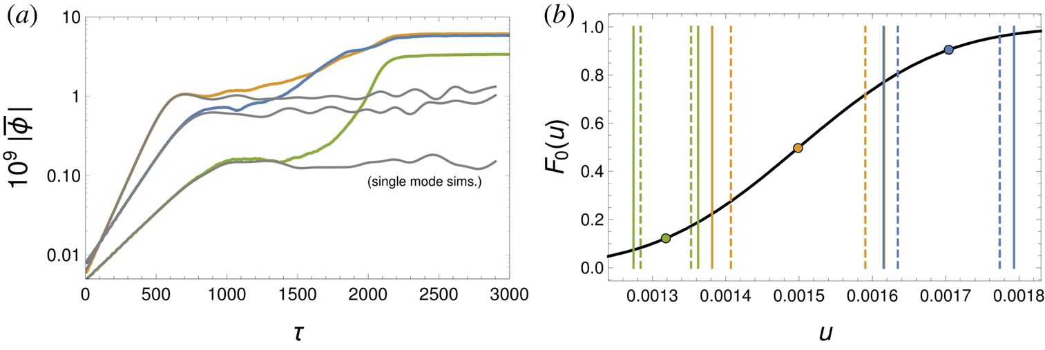In the considered case, the onset of the overlap regime at saturation time emerges for $\eta \geqslant 0.00055$, as clearly represented by the mode evolution depicted in figure 2(a). The system is evolved self-consistently for the three modes and it is compared with the single-mode simulation results of each resonance (grey lines). As can be argued from the plot, two resonances start to interact nearby the corresponding single-mode saturation time. In particular, by increasing the value of $\eta$, the resonances become increasingly more overlapped and the interaction time becomes smaller. On the contrary, reducing the drive results in a progressive separation of the resonances, which eventually behave as isolated. For small $\eta$, however, some residual nonlinear interplay is found, although the overlap starts much later than single-mode saturation time.

Figure 2.

(a) Plot of the mode evolution in a three-resonance model (coloured lines) and the respective single-mode simulations (grey lines), for $\eta =0.00055$. The colour scheme is: $u_{\textrm {r}1}\simeq 0.0013$ (green), $u_{\textrm {r}2}\simeq 0.0015$ (yellow), $u_{\textrm {r}3}\simeq 0.0017$ (blue). (b) Three-resonance system. The black line represents $F_0$ of (2.2). Circles denote $u_{\textrm {r}1}$ (green), $u_{\textrm {r}2}$ (yellow) and $u_{\textrm {r}3}$ (blue). We indicate also $u_{\textrm {r}}\pm \Delta u^{c}_{\textrm {NL}}$(dashed lines) and $u_{\textrm {r}}\pm \Delta u_{\textrm {NL}}$ (solid lines) with corresponding colours.

Let us now depict the resonance position and the corresponding $\Delta u^{c}_{\textrm {NL}}$ (figure 2b, dashed lines) for the threshold value $\eta =0.00055$. In this case, the nonlinear trapping regions appear, actually, non-overlapped, suggesting that fluctuations should evolve as superposition of non-interacting modes. Such evidence has the physical implication that in the ‘active’ overlap of different nonlinear fluctuations, also particles that are not trapped by the wave (Elskens & Escande Reference Elskens and Escande2003) are relevant. This phenomenon is related to the analysis of the transition to stochasticity of adjacent resonances. There is a vast literature on this specific topic and the corresponding well-known Chirikov overlap criterion (Chirikov Reference Chirikov1960, Reference Chirikov1979) (for details, see also Escande & Doveil (Reference Escande and Doveil1981), Berk et al. (Reference Berk, Breizman and Pekker1995b) and Lichtenberg & Lieberman (Reference Lichtenberg and Lieberman2010)). It is worth remarking that in the present work, the fluctuating spectrum is not imposed, as usual (Elskens & Escande Reference Elskens and Escande2003; Lichtenberg & Lieberman Reference Lichtenberg and Lieberman2010), as an external field. It is instead self-consistently determined including also the coupled beam particle nonlinear evolution, as in the already mentioned works related to the threshold drive for the onset of overlapping. According to the literature (e.g. Lichtenberg & Lieberman Reference Lichtenberg and Lieberman2010), the quantity $\Delta u^{c}_{\textrm {NL}}$ must be enlarged by means of a scale factor to obtain the observed overlap of the resonance width. In particular, taking into account figure 2(b), we have to multiply the clump widths evaluated using $\Delta u^{c}_{\textrm {NL}}=6.64 \bar {\gamma }_{\textrm {L}}$ (dashed lines) by a factor ${>}1$ in order to obtain a non-zero intersection of the new re-sized nonlinear spread regions (solid lines). In our case, this is represented by the yellow/blue line intersection around $u=0.00162$. We can thus recognize an effective nonlinear velocity spread $\Delta u_{\textrm {NL}}$, able to properly describe the verified resonance regime, as

(3.1)\begin{equation} \Delta u_{\textrm{NL}}=\beta\Delta u^{c}_{\textrm{NL}},\quad\beta\simeq1.28, \end{equation}

well represented in the figure with solid lines.

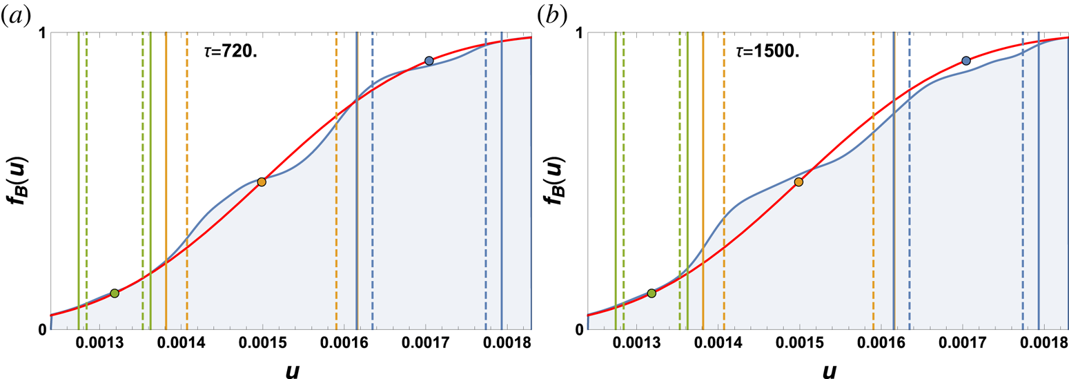
It is worth observing that, for the obtained $\beta$ value, the resonance $u_{\textrm {r}1}$ (represented in green) results in being initially isolated even using the redefined nonlinear width. Nonetheless, in this scenario, the nonlinear interplay of the overlapping resonances ($u_{\textrm {r}2}$ and $u_{\textrm {r}3}$) affects the dynamics by broadening the corresponding region of nonlinear velocity spread (as discussed in Berk & Breizman (Reference Berk and Breizman1994) and Berk et al. (Reference Berk, Breizman and Pekker1994, Reference Berk, Breizman and Pekker1995b)). This can be recognized in the evolution of the distribution function $f_{\textrm {B}}(u,\tau )$ plotted in figure 3. The initial merging at saturation time of the second two resonances (yellow and blue) is evident, while for later times the morphology of the distribution profile starts to affect the resonance region of the first (green) resonance. In this way, the $u_{\textrm {r}1}$ overlap sets in at this slightly later time (cf. also figure 2a), after the other fluctuations have been nonlinearly amplified. This eventually allows synergistic interaction also with the initially isolated resonance. We also mention that, setting a system in which only the first two resonances $u_{\textrm {r}1}$ (green) and $u_{\textrm {r}2}$ (yellow) are considered, it can be shown how (for the sake of simplicity, we do not propose other plots) they properly behave as two independent modes as predicted by the quantity $\Delta u_{\textrm {NL}}$ in (3.1).

Figure 3.

Beam distribution function at saturation $f_{\textrm {B}}(u,\tau _{\textrm {S}}=720)$ (a) and at a later instant $f_{\textrm {B}}(u,\tau =1500)$ (b) for $\eta =0.00055$ in the case of three resonances. Colour scheme and other notations as in figure 2(b). The red line represents $F_0$.

A careful analysis of the BPS is developed in Berk et al. (Reference Berk, Breizman and Pekker1995b), where different regimes of the dynamics are considered and numerical simulations are shown to be in agreement with the theoretical models (Berk, Breizman & Ye Reference Berk, Breizman and Ye1992; Breizman, Berk & Ye Reference Breizman, Berk and Ye1993; Berk & Breizman Reference Berk and Breizman1994; Berk et al. Reference Berk, Breizman and Pekker1994), e.g. the pulsating regime. The present re-analysis emphasizes the role played by intrinsic nonlinear effects, due to the self-consistent evolution of the system. Actually, the clump size is typically fixed via analytical estimates, which break down the self-consistency by assuming a frozen field. In Carlevaro, Finelli & Montani (Reference Carlevaro, Finelli and Montani2019a), it has been clearly shown how retaining this self-consistency is of crucial importance to ensure predictivity. Here, we also argue how the overlapping process of two or more resonances can strictly depend on small deformations of the distribution function in those regions of the velocity space which are out of the plateau. Such apparently marginal deformations contribute to the real size of the resonant region and play a crucial role when the BPS is implemented into the dynamics of fast ions in the Alfvén spectrum of a fusion device (Berk & Breizman Reference Berk and Breizman1990a,Reference Berk and Breizmanb,Reference Berk and Breizmanc).

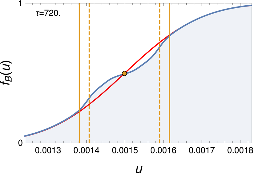
In view of the study of the next section, we conclude by analysing the morphology of the beam distribution function in the presence of only the single resonance $u_{\textrm {r}2}$ (the saturation time is set at $\tau _{\textrm {S}}=720$). The results are summarized in figure 4. The role of non-trapped particles is clear in this scheme: the re-sized nonlinear velocity spread $\Delta u_{\textrm {NL}}$ well defines the global distortion of $f_{\textrm {B}}(\tau _{\textrm {S}})$ with respect to the initial profile $F_0$, including non-trapped but nearly resonant particles. These are represented by the plateau edges, which is relevant in the active overlap.

Figure 4.

Snapshot of the beam distribution function at saturation $f_{\textrm {B}}(u,\tau _{\textrm {S}}=720)$ for $\eta =0.00055$ in the presence of one single resonance $u_{\textrm {r}2}$, represented by the circle (red line represents $F_0$). We also indicate $u_{\textrm {r}}\pm \Delta u^{c}_{\textrm {NL}}$ (dashed lines) and $u_{\textrm {r}}\pm \Delta u_{\textrm {NL}}$ (solid lines).

The present study provides an example regarding the difficulty of having quantitative predictions for the degree of overlap based on the linear parameters (the system drive). The physical impact of this fact relies on the possibility of discriminating or excluding specific transport regimes directly from the linear set-up in order to apply (or not) reduced schemes for the dynamics. The focus on the saturation time is due to the necessity of applying the standard estimate for the particle trapping dynamics. Moreover, this choice is also natural because at the saturation time the field amplitude approaches a constant value and we can compare this picture with the case of an assigned external field. Only slightly different results could be obtained by setting later times and/or extending the time scale for the mixing of the phase space to occur.

We conclude this section by stressing how this analysis of the beam–plasma instability refines in a fully-self consistent fashion (also using more realistic profiles for the particle distribution) the already existing studies regarding the transition to stochasticity made by dynamical system theory. In particular, using the scaling addressed in the previous section, we get

(3.2)\begin{equation} \Delta u_{\textrm{NL}}/u_{\textrm{r}}\simeq8.5\;\bar{\gamma}_{\textrm{L}}. \end{equation}

This expression provides a prescription about the resonance width directly from linear information and it is able to properly describe the resonance overlap regimes, improving the estimates of the trapping region related to the mode saturation amplitude.

4 Lagrangian coherent structure analysis

Let us now describe phase-space dynamics produced by resonance overlap using the LCS technique, in comparison to the distribution profile evolution of figures 3 and 4. Lagrangian coherent structures are a generalization of dynamical structures observed in autonomous and periodic systems, e.g. invariant manifolds, to temporally aperiodic flows and allow one to identify phase-space regions distinguished by qualitatively different behaviour of particle motion (see Haller (Reference Haller2015), Falessi, Pegoraro & Schep (Reference Falessi, Pegoraro and Schep2015), Carlevaro et al. (Reference Carlevaro, Falessi, Montani and Zonca2015), Di Giannatale et al. (Reference Di Giannatale, Falessi, Grasso, Pegoraro and Schep2018a,Reference Di Giannatale, Falessi, Grasso, Pegoraro and Schepb) and Pegoraro et al. (Reference Pegoraro, Bonfiglio, Cappello, Di Giannatale, Falessi, Grasso and Veranda2019) for applications to plasma physics). Following the work of Haller (Reference Haller2015), we define LCSs as the most repulsive or attractive material lines (one-dimensional ensemble of material points, i.e. points advected by the dynamics) with respect to the nearby ones and, therefore, they are associated with peaked profiles of the finite-time Lyapunov exponent (FTLE) fields.

In order to calculate the FTLE fields, we trace several test particle trajectories under the action of the time-dependent scalar potential generated from an $N$-body simulation. Test particles are initialized to sample the whole phase space of interest, at a fixed time $\tau$, in two phase-space grids having an infinitesimal displacement in the velocity direction. In other words, a test particle located in $(\bar {x},u)$ has a neighbour initialized in $(\bar {x},u+\delta _\tau )$. Evolving such a system with assigned time-dependent potentials, at a time $\tau +{\rm \Delta} \tau$ these two test particles will be at a distance $\delta _{{\rm \Delta} \tau }$ in the phase space and the FTLE value $\sigma$ in the point $(\bar {x},u)$ can be evaluated using the following expression:

(4.1)\begin{equation} \sigma(\bar{x},u,\tau,{\rm \Delta} \tau)= \ln (\delta_{{\rm \Delta} \tau}/\delta_\tau)/{\rm \Delta} \tau. \end{equation}

When considering a positive time span ${\rm \Delta} \tau >0$, the curves where the FTLE field is peaked define repulsive transport barriers, while when setting ${\rm \Delta} \tau <0$ they represent attractive ones. The LCS can be visualized by plotting the maximum values of 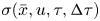$\sigma (\bar {x},u,\tau ,{\rm \Delta} \tau )$ as extracted from a contour plot in the phase space. In the analysis of this section, we have set two grids of $200\times 200$ test particles, thus obtaining 4000 values of the FTLE for each phase-space snapshot. We apply the methodology introduced in Carlevaro et al. (Reference Carlevaro, Falessi, Montani and Zonca2015) and we choose a relatively small value for $\Delta \tau$ which highlights finite-time transport barriers instead of the system asymptotic properties such as invariant manifolds. The scalar electrostatic potentials have been sampled from the complete $N$-body simulations.

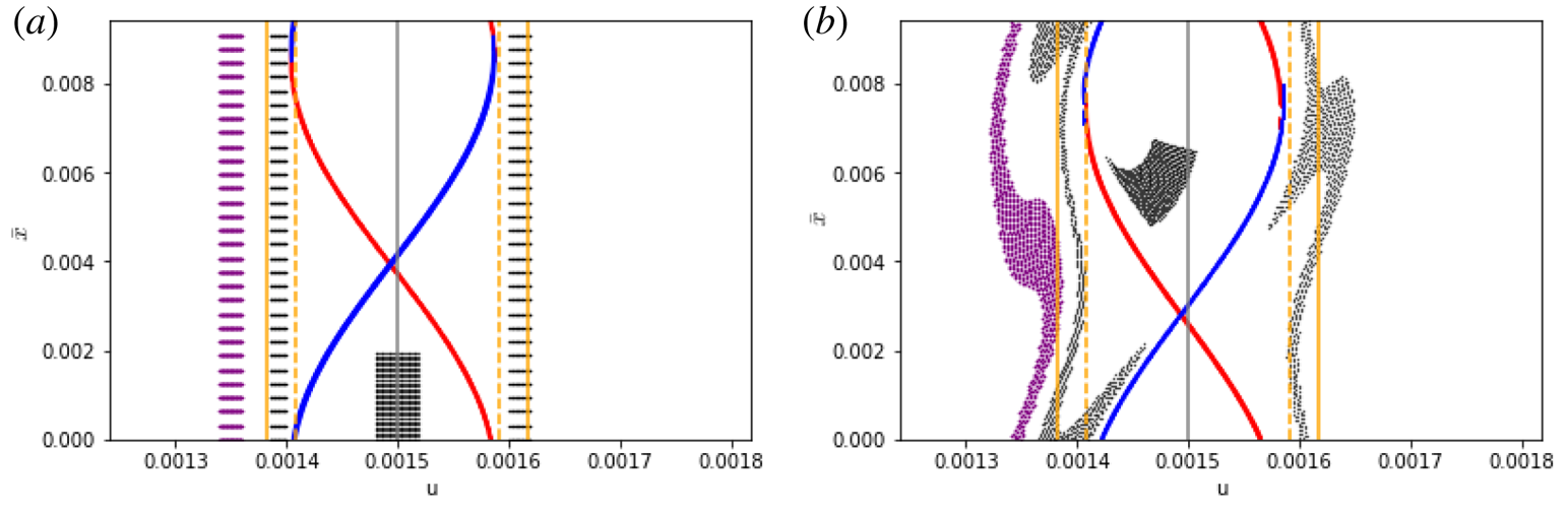
We first characterize phase-space dynamics in the presence of one mode with resonance velocity $u_{\textrm {r}}=0.0015$. In figure 5, we show attractive and repulsive transport barriers (in blue and red, respectively) associated with a time span of $\Delta \tau = 20$ together with a collection of tracers at two different snapshots, i.e. $\tau = 700$ and $800$, to underline the saturation dynamics (cf. figure 4). Yellow lines are placed at $u_{\textrm {r}} \pm \Delta u^{c}_{\textrm {NL}}$ and $u_{\textrm {r}} \pm \Delta u_{\textrm {NL}}$, as indicated in the figure caption. As expected, the phase space is divided into different macro-regions with negligible exchange of particles between them representing the inside and the outside, respectively, of a clump which moves coherently, i.e. only with just minor deformation of its structure. This dynamics is confirmed by the evolution of the tracers and can be attributed to the relatively low-amplitude oscillations of the electric field around its saturation value. In particular, as shown in Carlevaro et al. (Reference Carlevaro, Falessi, Montani and Zonca2015), greater amplitude oscillations of the scalar potential can de-trap a fraction of the particles originally inside the clump and vice versa. The value of $\Delta u^{c}_{\textrm {NL}}$ is consistent with the maximum velocity width of the region enclosed by the LCS. Tracers outside $u_{\textrm {r}} \pm \Delta u_{\textrm {NL}}$ have been coloured in order to highlight their dynamics. It can be argued how these particles are exchanging, on average, less power with respect to those ones in the inside region which are moving towards the $x$ point consistent with the already introduced resonance width.

Figure 5.

Attractive and repulsive LCSs (in blue and red, respectively) in the presence of one resonant mode ($u_{\textrm {r}}\simeq 0.0015$), marked by a grey line, calculated by means of the FTLE field with $\Delta \tau = 20$ at $\tau = 700$ (a) and $\tau =800$ (b). Dashed lines are placed at $u_{\textrm {r}} \pm \Delta u^{c}_{\textrm {NL}}$ while solid ones at $u_{\textrm {r}} \pm \Delta u_{\textrm {NL}}$ (cf. figure 4). Passive tracers are depicted with different colours to show phase-space dynamics.

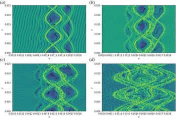
The same technique can be applied to describe the resonance overlap process introduced in § 3. In figure 6 (cf. the evolution of the distribution function in figure 3) we show, for each point of the phase space, the largest FTLE value obtained by either a forward or a backward time integration with $\Delta \tau = {\pm }20$. We plot, for the sake of clarity, attractive and repulsive LCSs with the same colour since this difference is not relevant for the present analysis. For $\tau =700$, three closed domains are depicted, while trajectories characterized by $u \lesssim 0.0013$ and $u \gtrsim 0.0017$ are only slightly deformed. The three resonances do not behave independently, thus generating overlap at saturation time as described in the previous section and the LCS technique allows one to illuminate this dynamics at each time step. In particular, in figure 6(a), even if the clumps look undistorted and the scalar potentials have approximately single-mode simulation values, the FTLE profile shows peaked structures in the region between adjacent resonances, i.e. $u_{\textrm {r}} \sim 0.0015$ and $u_{\textrm {r}} \sim 0.0017$, thus suggesting transport processes in the phase space (for a detailed description of this process, see Carlevaro et al. (Reference Carlevaro, Falessi, Montani and Zonca2015)). The overlap is more evident in the next two snapshots ($\tau =1100$ and $1500$), where this region is filled by a convoluted tangle of repulsive and attractive structures. In the last snapshot ($\tau =2100$), the overlap is complete and a unique structure is formed consistent with the formation of a plateau in the particle distribution function.

Figure 6.

Contour plots of the FTLE value obtained either with a forward or with a backward time integration ($\Delta \tau = {\pm }20$) at $\tau = 700$ (a), $1100$ (b), $1500$ (c) and $2100$ (d). Regions with high FTLE are represented in yellow (colour scheme from blue to yellow). Passive tracers are marked in black.

5 Mode amplitude at saturation

The case analysed in the previous sections corresponds to an intermediate situation between the limiting cases of isolated and strongly overlapping resonances. Figure 2(a) shows that the mode saturation levels are larger in the multi-mode simulations than in the single-mode runs. This feature of the BPS has been discussed in Berk et al. (Reference Berk, Breizman and Pekker1995b) (see also references therein), where sources and sink are included in the model. Due to the enhancement of the distribution function plateau in the overlapping regime, the amount of free energy of the interaction process becomes larger, and this is the cause of the observed mode saturation level.

In the following, we numerically show the overlapping saturation as a function of the phase-velocity separation of neighbouring modes, highlighting the feature mentioned above in the collisionless case. Equivalent to the conclusion drawn in Berk et al. (Reference Berk, Breizman and Pekker1995b), we provide a visual interpretation of this process in terms of the areas relative to the distribution function distortions, i.e. the particle number. In particular, we initialize the beam particles using a distribution function with a positive constant gradient and $\eta =0.002$, i.e. we consider a linear initial profile in the velocity space. We run seven simulations with two modes, fixing one of the resonances (namely at $u_{\textrm {r}1}=0.00135$) and sweeping the other one (dubbed $u_{\textrm {r}2}$) in order to span, with constant velocity increment, the resonance separations $\Delta u_{\textrm {SEP}}\equiv u_{\textrm {r}2}-u_{\textrm {r}1}$ from $5\times 10^{-6}$ to $2\times 10^{-3}$. For each case, we compare numerical results with the evolutions obtained for isolated resonances.

In the presence of multiple modes and resonances, we recall that the total momentum and energy are conserved. In particular, total conserved momentum can be written as (O'Neil et al. Reference O'Neil, Winfrey and Malmberg1971; Carlevaro et al. Reference Carlevaro, Falessi, Montani and Zonca2015)

(5.1)\begin{equation} \mathcal{K}_{\textrm{P}}=\sum_{\ell}\frac{|\bar{\phi}_{\ell}|^{2}}{\ell}+\frac{2}{\eta N}\sum_i u_i. \end{equation}

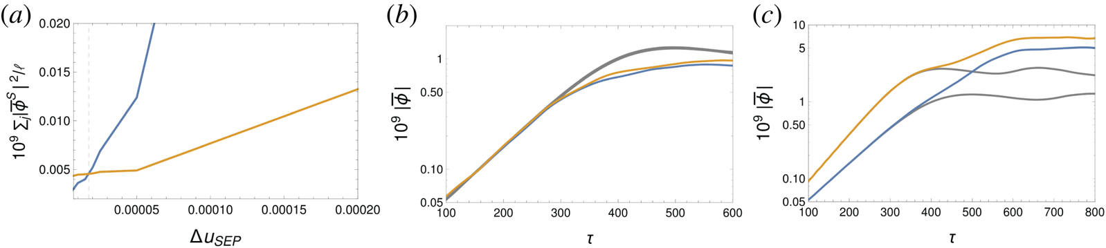
Thus, for each case, we can measure the saturation level as $\sum _\ell |\bar {\phi }_{\ell }^S|^{2}/\ell$. In figure 7 (a), we plot an interpolation of this quantity as function of $\Delta u_{\textrm {SEP}}$ for the self-consistent simulations of two modes (blue line) compared with the saturation levels obtained artificially superposing the evolution of isolated resonances (yellow line). Note that for vanishing resonance separation, as expected, the self-consistent saturation level is half of the value obtained by the artificial addition of single isolated modes. In fact, for coalescing resonances, the modes become different realizations of the same fluctuating field and their saturation amplitude is reduced by a factor of two. It is immediately seen that a threshold value ($\Delta u^*_{\textrm {SEP}}\simeq 1.75\times 10^{-5}$) emerges, below which the saturation level for the self-consistent evolution is lower than that obtained by artificial superposition of single isolated modes: this corresponds to the regime of strongly overlapped resonances. The opposite situation occurs above $\Delta u^*_{\textrm {SEP}}$ (clearly provided that $\Delta u_{\textrm {SEP}}\lesssim 2\Delta u^{\textrm {f}}_{\textrm {NL}}$, otherwise resonances are not overlapped and the modes evolve as single isolated fluctuations). In order to better illustrate such a behaviour, in figure 7 we also plot the single- and multi-mode evolutions, for a case below (figure 7b) and above (figure 7c) threshold, respectively.

Figure 7.

(a) Saturation level $\sum _\ell |\bar {\phi }_{\ell }^S|^{2}/\ell$ as a function of $\Delta u_{\textrm {SEP}}=u_{\textrm {r}2}-u_{\textrm {r}1}$ for self-consistent simulations of two resonances (blue) compared with the saturation level obtained artificially superposing the evolution of the individual isolated resonances (yellow). The threshold for the onset for enhanced saturation level is the intersection point (dashed grey line) $\Delta u^*_{\textrm {SEP}}\simeq 1.75\times 10^{-5}$. (b,c) Time evolution of the modes for the multi-mode (coloured lines) and single-mode (grey lines) systems for a case below threshold, i.e. $\Delta u_{\textrm {SEP}}\simeq 5.5\times 10^{-6}$ (b), and above threshold, i.e. $\Delta u_{\textrm {SEP}}\simeq 2\times 10^{-4}$ (c).

5.1 Interpretative model

When the multi-mode saturation level is larger than for single isolated modes, it is evident that a more efficient process can tap energy from the particle phase space. Following the line of Berk et al. (Reference Berk, Breizman and Pekker1995b), we discuss a toy model to qualitatively describe this effect and the threshold condition introduced above.

For each resonance, respectively called $u_1$ and $u_2$, we assume to model the nonlinear distorted distribution function at saturation by a flattening over a certain region; that is, as horizontal lines centred at the resonance position and extended over twice the nonlinear velocity spread, respectively denoted as $\Delta u_1$ and $\Delta u_2$ for the two considered resonances. As described in the previous sections, resonance overlap occurs when the flattening regions intersect. We then describe the overlapping resonances as a single one having a new resonance velocity and nonlinear velocity spread defined, respectively, by

(5.2)\begin{equation} u_{\textrm{r}}=u_1+\Delta u_{\textrm{SEP}}/2 \end{equation}

and

(5.3)\begin{equation} \Delta u_{\textrm{r}}=\rho((u_2+\Delta u_2)-(u_1-\Delta u_1))/2, \end{equation}

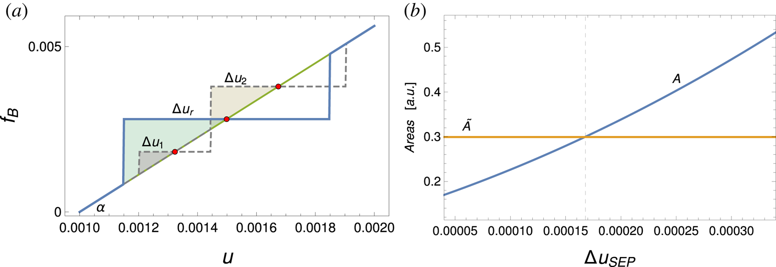
where $\Delta u_{\textrm {SEP}}=u_2-u_1$ and $\rho =\textit{O}(1)$ is a control parameter for the model. This scheme is illustrated, for $\rho =1$, in figure 8 (a), where we used realistic quantities (estimated from $\Delta u_{\textrm {NL}}$) for comparison with the simulation results described above.

Figure 8.

(a) Representation for the distribution function at saturation in the case of single isolated modes (grey dashed lines) and of one overlapped resonance (blue solid line) modelled using (5.2) and (5.3). Red dots correspond, from left to right, to $u_1$, $u_{\textrm {r}}$ and $u_2$, respectively. Corresponding velocity spreads are indicated in the plot. (b) Behaviour of $\tilde {A}$ (yellow) and $A$ for $\rho =1$ (blue) in terms of $\Delta u_{\textrm {SEP}}$. Dashed grey line indicates the intersection point.

The nonlinear mode saturation corresponds to particle transfer from large to small velocities as indicated in the momentum conservation law (5.1). Thus, the relevant quantities to be analysed are the areas of the triangles that are coloured in the figure. These correspond to the amount of available free energy, in the interpretation of Berk et al. (Reference Berk, Breizman and Pekker1995b). Evolving the two modes as single isolated resonances, the saturation level scales as

(5.4)\begin{equation} \tilde{A}= \tan\alpha((\Delta u_1)^2+(\Delta u_2)^2)/2, \end{equation}

i.e. as the sum of the areas built around the two resonances. Here $\alpha$ denotes the angular coefficient of the initial linear distribution. Meanwhile, the area of the triangle corresponding to the new merged resonance can be evaluated by means of (5.2) and (5.3) as

(5.5)\begin{equation} A=\rho^2 \tan\alpha(\Delta u_{\textrm{SEP}}+\Delta u_1+\Delta u_2)^2/8. \end{equation}

Assuming to neglect the velocity dependence of $\Delta u_2$ (as $u_2$ is swept to change $\Delta u_{\textrm {SEP}}$), figure 8 (b) shows $\tilde {A}$ and $A$ (for $\rho =1$) as functions of the resonance separation.

For $\Delta u_{\textrm {SEP}} > \Delta u_1 + \Delta u_2$ there is no resonance overlap and the system response is consistent with two isolated resonances. For decreasing $\Delta u_{\textrm {SEP}}$ below the onset of the overlap (i.e. the system depicted in 8a), the saturation level for the merged resonance is larger than for the single isolated modes, i.e. $A>\tilde {A}$, or, more precisely, $A=2\tilde {A}$ at the onset condition, suggesting a sudden transition in the nonlinear dynamics due to the synergistic behaviour of the interacting modes. In particular, it is readily verified that $A>\tilde {A}$ as long as a lower critical threshold is exceeded (as in the simulation results), namely

(5.6)\begin{equation} \Delta u_{\textrm{SEP}}^*=-\Delta u_1-\Delta u_2+2\sqrt{((\Delta u_1)^2+(\Delta u_2)^2)/\rho^2}. \end{equation}

Thus, we can identify a range for enhanced or synergistic interaction of overlapping resonances

(5.7)\begin{equation} \Delta u^*_{\textrm{SEP}}<\Delta u_{\textrm{SEP}}<\Delta u_1 + \Delta u_2. \end{equation}

Meanwhile, for $\Delta u_{\textrm {SEP}}<\Delta u^*_{\textrm {SEP}}$, the two resonances are strongly overlapping and $A<\tilde {A}$, with $A=\tilde {A}/2$ in the limit of $\Delta u_{\textrm {SEP}}=0$. This is consistent with our numerical simulations.

The discrepancy between the intersection point ($\simeq 1.7\times 10^{-4}$) of figure 8 (b) with respect to the value found in numerical simulations shown in figure 7 (a) is due to intrinsic details of the nonlinear evolution and the simplification contained in the model: it can be taken into account by properly setting the model control parameter $\rho$. Indeed, a proper match of the model theoretical threshold with numerical simulations can be obtained using $\rho =1.41$. As a result, the present model shows how the mode saturation level can be described via the analysis of wave–particle power transfer in phase space. The model can also be made quantitative (and, thus, predictive) by a proper choice of the control parameter $\rho$.

6 Concluding remarks

The BPS and its paradigmatic implications in plasma and fusion physics have been widely discussed across the literature. The present analysis focused on the refinement of some subtle questions mandatory for practical applications, in order to make quantitative estimates of the nonlinear wave–particle interaction.

A study of the nonlinear velocity spread allowed selection of a proper region in the velocity space characterizing the resonance width. Analysing the simulations of isolated resonances up to the limiting distance of their overlap, we show that also the ‘tails’ around the plateau play an important dynamical role. It is worth noting that such regions do not contain trapped particles. Nonetheless, their existence must be carefully taken into account when assessing the separation of two resonant modes. In fact, the plateau region, mainly coinciding with the clump size in the phase space, would underestimate the transport of particles between two adjacent resonances due to the important role played by non-trapped particles. The shape of the clumps and phase-space dynamics have been described using the LCS technique, which clarifies how particles outside the effective resonance width exchange limited power with the mode spectrum.

Finally, we study the enhanced saturation of interacting resonant modes with respect to the level of isolated resonances. We quantitatively describe the merging/overlap of two adjacent resonances. A critical distance exists in the velocity space, above which the two resonances are isolated and below which they are too overlapped to be really distinct in the velocity space. In either case, the two fluctuations behave as individual modes and the wave–particle power exchange is limited. Only when the two resonances are adjacent and the power transfer from particles to modes is maximized by an enforced velocity spread (essentially the sum of the original ones) can we predict the enhanced saturation observed for instance in Schneller et al. (Reference Schneller, Lauber and Briguglio2016) and Vlad et al. (Reference Vlad, Briguglio, Fogaccia, Fusco, Di Troia, Giovannozzi, Wang and Zonca2018).

The analysis of this paper offers a summary of the relevant features of the bump-on-tail paradigm (to which the BPS is isomorphic), in view of its paradigmatic character in describing several important physical problems. Quantitative prediction of resonance overlap and of enhanced saturation conditions and levels was the original motivation of this work, which has led us to conclude that the system evolution is strongly influenced by the global features of the distribution function.