





Highlights
What is already known?
-
• Several common models are used in meta-analysis, including the fixed-effect (or common effect), random-effects, and mixed-effects models.
-
• Structural equation modeling (SEM) has been proposed to represent these models, a concept referred to as SEM-based meta-analysis in the literature.
What is new?
-
• This tutorial extends SEM-based meta-analysis to accommodate complex meta-analytic models, such as the multiplicative error model (or unrestricted weighted least squares model), the hybrid of additive and multiplicative error models, and the location-scale model.
-
• It also demonstrates how to specify and analyze these complex meta-analytic models among effect sizes, which may include linear and nonlinear constraints, using SEM language in R.
Potential impact for RSM readers
-
• RSM readers will not only learn about meta-analytic models through equations and algorithms, but can also explore these models through graphical representations.
-
• RSM readers can specify novel meta-analytic models that may not yet be implemented in their preferred software, enabling them to effectively address their research questions.
1 Introduction
Meta-analysis is a powerful tool for synthesizing research findings in various disciplines, including psychology,Reference Rosenthal and DiMatteo 1 management,Reference Morris 2 public health,Reference Tanner-Smith and Grant 3 and medical science,Reference Sutton 4 among others. The significance of meta-analysis in scientific research is underscored by several dedicated journals, including Psychological Bulletin, Review of Educational Research, Neuropsychology Review, and Cochrane Reviews, which prioritize the publication of systematic reviews and meta-analyses. Research Synthesis Methods publishes papers related to systematic reviews and meta-analyses and contributes to methodological advancements in this field. Historically, the fixed-effect model, also known as the common- or equal-effects model, was widely employed in meta-analysis; however, its limitations have since been recognized. For instance, the findings are only generalized to the studies included in the meta-analysis. The estimated standard errors (SEs) are underestimated when the goal is to generalize beyond the studies included and the effect sizes are not homogeneous.
Today, the random-effects and mixed-effects models are the most commonly used in contemporary meta-analyses. The random-effects model posits that the variability in effect sizes between studies is due to some unknown random factors and sampling error. In the presence of excess heterogeneity, the mixed-effects model incorporates moderators or covariates to account for this heterogeneity. Recently, alternative meta-analytic models, such as the multiplicative error model (or unrestricted weighted least squares [UWLS] model), hybrid models combining additive and multiplicative error terms, location-scale models, and nonlinear models, have been proposed and increasingly applied in the literature.
These advanced models are typically presented using equations and algorithms to obtain parameter estimates and the SEs, requiring a strong statistical background to understand and implement. Researchers using these models often need to wait for these models to be implemented in programming languages, such as R, Python, or Stata. Although some popular meta-analysis tools, such as the metafor packageReference Viechtbauer 5 in R, 6 offer valuable functionalities, customizing these models for specific research purposes can still pose significant challenges.
Structural equation modeling (SEM) is a widely used framework to analyze latent and observed variables. It offers several attractive features. One of them is the ability to represent models graphically, which facilitates the clear communication of statistical models and their underlying assumptions. This graphical representation enables readers to quickly grasp the core concepts of the models without requiring advanced mathematical knowledge. Moreover, rather than mastering specific estimation methods or algorithms for each model, readers may learn a general estimation method, such as the full information maximum likelihood (FIML) estimation.
In a series of papers, CheungReference Cheung 7 – Reference Cheung and Hoyle 12 introduced the SEM-based meta-analysis to analyze univariate, multivariate, and three-level meta-analytic models as structural equation models. He demonstrated how to use SEM packages like OpenMx Reference Boker, Neale and Maes 13 , Reference Neale, Hunter and Pritikin 14 in R and Mplus Reference Muthén and Muthén 15 to perform meta-analyses. This SEM-based meta-analysis has been implemented in the metaSEM packageReference Cheung 16 in R. The present tutorial builds on this work by extending the applications of SEM to more advanced meta-analytic models, providing a guide on specifying, visualizing, and analyzing various common and advanced meta-analytic models as structural equation models in R.
This tutorial addresses two significant research gaps in the meta-analysis literature. First, it aids researchers in learning and understanding various meta-analytic models and their underlying assumptions by using a graphical modeling approach. In these models, there is a direct correspondence between graphical representations, equations, and matrix forms, simplifying the teaching and learning of meta-analysis without the need for complex equations. Second, it empowers researchers to fit a range of meta-analytic models in R. This approach also allows for the customization of novel models to include antecedents and consequences on effect sizes, offering researchers the flexibility to specify their own meta-analytic models. The SEM-based meta-analysis offers a straightforward yet powerful means to implement and test novel research questions in meta-analysis.
The tutorial begins with an overview of SEM. It then guides users through the specification of common meta-analytic models within the SEM framework, including the fixed-effect and random-effects models, multiplicative-error models, and hybrid models that combine additive and multiplicative errors. Next, it covers models with covariates and complex models, such as location-scale and nonlinear models. Then, it illustrates how this approach can tailor models that do not fit traditional meta-analysis frameworks, including regression models among effect sizes. The tutorial includes examples that demonstrate these procedures using the metaSEM package,Reference Cheung 16 which uses the OpenMx,Reference Neale, Hunter and Pritikin 14 lavaan,Reference Rosseel 17 and semPlot Reference Epskamp 18 packages in the backend, and the symSEM package.Reference Cheung 19 Finally, it discusses the limitations and potential future extensions of this approach. While this tutorial includes the mathematical models and assumptions of the associated meta-analytic models, it is essential to note that understanding these mathematics is not compulsory. Readers can also grasp these concepts by studying the graphical representations.
2 Brief introduction of structural equation modeling
In SEM, observed variables are represented by rectangles (or squares), while latent variables are represented by ellipses (or circles). We may represent the means or intercepts with triangles with a “1” inside, indicating columns of ones. Once we have variables, we may hypothesize their relationship by linking them with single or double arrows. Single arrows represent direct paths, like regression coefficients or factor loadings; double arrows represent covariances or variances (see the
$\boldsymbol {A}$
 and
$\boldsymbol {S}$
 matrices in the next paragraph).
These graphical elements have a direct correspondence to model equations. Each single-headed arrow pointing into a variable contributes one term to its equation of the form: coefficient
$\times $
 source variable. For example, in Figure 1(a), two arrows enter an effect size
$y_i$
 : one from the intercept triangle (constant “1”) with coefficient
$\mu $
 , and one from the latent variable
$e_i$
 with coefficient 1. Reading these arrows directly gives the model equation
$y_i = \mu \cdot 1 + 1 \cdot e_i = \mu + e_i$
 . This graphical-to-equation correspondence is illustrated below using the fixed-effect model as a fully worked example; readers are then invited to apply the same logic when inspecting subsequent path diagrams throughout the tutorial.
Structural equation models of fixed- and random-effects models.
Note: Figure (a) illustrates a fixed-effect (or common-effect) model. Panels (b) and (c) depict a random-effects model that incorporates additive heterogeneity error. The sampling error
$e_i$
 is conceptualized as a latent variable in Figures (a) and (b) and as measurement error in Figure (c). Here,
$y_i$
 represents the effect size for the ith study, while
$data.vi$
 indicates its known sampling error variance. Additionally,
$u_i$
 stands for the random effect with
$\tau ^2$
 representing the heterogeneity variance. Furthermore,
$\mu $
 denotes the average effect (or common effect in the fixed-effect model).

Figure 1 Long description
The diagram consists of three panels labeled A, B, and C.
Panel A (Fixed-effect model): A circle labeled e sub i with a self-loop labeled data dot v i points to a shaded rectangle labeled y sub i with a path coefficient of 1. A triangle containing the number 1 points down to y sub i with a path coefficient of mu.
Panel B (Random-effects model): Two circles on the left, u sub i and e sub i, both point to a shaded rectangle y sub i with path coefficients of 1. The circle u sub i has a self-loop labeled tau-squared. The circle e sub i has a self-loop labeled data dot v i. A triangle containing the number 1 points down to y sub i with a path coefficient of mu.
Panel C (Random-effects model with measurement error): A circle labeled u sub i with a self-loop labeled tau-squared points to a shaded rectangle y sub i with a path coefficient of 1. The rectangle y sub i has its own self-loop labeled data dot v i. A triangle containing the number 1 points down to y sub i with a path coefficient of mu.
Structural equation models are typically specified using equations due to their convenience and clarity. The lavaan syntax,Reference Rosseel
17
inspired by Mplus, is a popular choice in R. Readers unfamiliar with the lavaan syntax may refer to lavaan’s website for an introduction. After a structural equation model is specified, most SEM packages automatically convert the equations to matrices to facilitate the computations. The Reticular Action Model (RAM)Reference McArdle and McDonald
20
is a powerful formulation for representing SEM models. Suppose that
$p_o$
 is the number of observed variables,
$p_l$
 is the number of latent variables in the model, and
$p = p_o + p_l$
 is the total number of variables. Four matrices are sufficient to specify most structural equation models in RAM:
-
1. The $\boldsymbol {A} p \times p$
 matrix represents asymmetric paths from variables in columns to variables in rows, such as regression coefficients and factor loadings.
-
2. The $\boldsymbol {S} p \times p$
matrix represents symmetric paths, such as covariances and variances. -
3. The $\boldsymbol {M} p \times 1$
vector is used to represent the means and intercepts. -
4. The $\boldsymbol {F} p_o \times p$
filter matrix is used to select the observed variables.


Once the models are specified, SEM programs convert the proposed model into a model-implied covariance matrix
$\boldsymbol {\Sigma }_i(\boldsymbol {\theta })$
 and a model-implied mean vector
$\boldsymbol {\mu }_i(\boldsymbol {\theta })$
 in the ith subject (or study in a meta-analysis):

where
$\boldsymbol \theta $
 is a vector of the free parameters and I is a
$p \times p$
 identity matrix. It should be noted that there is a subscript i in
$\boldsymbol {\Sigma }_i(\boldsymbol {\theta })$
 ,
$\boldsymbol {\mu }_i(\boldsymbol {\theta })$
 , and
$\boldsymbol {F}_i$
 , indicating that the dimensions of
$\boldsymbol {\Sigma }_i(\boldsymbol {\theta })$
 ,
$\boldsymbol {\mu }_i(\boldsymbol {\theta })$
 , and
$\boldsymbol {F}_i$
 may vary across subjects (or studies in meta-analysis). This feature is essential as it allows the model to filter out data with missing values before analysis. Assuming the data are multivariate normal, the
$-2$
 *log-likelihood (
$-$
 2LL) for all K subjects–or studies in a meta-analysis–is:

where K is the number of subjects,
$k_i$
 is the number of complete observed variables, and
$\boldsymbol {y}_i$
 is the vector of observed data in the ith subject. The parameter estimates, denoted as
$\hat {\boldsymbol {\theta }}$
 , are derived by minimizing the
$-$
 2LL function. Once the model is fitted, the software provides a range of outputs, including parameter estimates, SEs, 95% Wald CIs, or likelihood-based confidence intervals (LBCIs),Reference Neale and Miller
21
and various fit statistics.
To make the RAM formulation concrete and accessible, we now work through the fixed-effect model in Figure 1(a) as a step-by-step illustration. This model contains
$p_o = 1$
 observed variable,
$y_i$
 (the rectangle), and
$p_l = 1$
 latent variable,
$e_i$
 (the ellipse), so there are
$p = p_o + p_l = 2$
 variables in total. Applying the lavaan2RAM function to the lavaan specification produces the following four RAM matrices, with variable names labeling all rows and columns:

Every non-zero entry has a direct counterpart in Figure 1(a):
-
• A matrix (single-headed arrows). The entry $\boldsymbol {A}[\text {row},\text {col}]$
records the coefficient of the directional path pointing from the column variable to the row variable. The single non-zero entry
$\boldsymbol {A}[y_i, e_i] = 1$
corresponds to the arrow from the ellipse
$e_i$
to the rectangle
$y_i$
with coefficient 1 in Figure 1(a). It encodes the contribution
$1 \times e_i$
to the equation for
$y_i$
. All other entries are zero because no other directional arrows exist in this model. -
• S matrix (double-headed arrows: variances and covariances). The entry $\boldsymbol {S}[\text {row},\text {col}]$
records the covariance between the row and column variables, or the variance when row
$=$
col. The single non-zero entry
$\boldsymbol {S}[e_i, e_i] = v_i$
corresponds to the curved double-headed loop on the ellipse
$e_i$
in Figure 1(a), encoding the sampling variance
$v_i$
of the ith study. Because
$v_i$
is a known constant that differs from study to study rather than a free parameter to be estimated, metaSEM reads it from the data via the definition variable data.vi, which will be introduced below. -
• F matrix (selecting observed variables). The $\boldsymbol {F}$
matrix has one row for each observed variable and one column for every variable in the model. The entry
$\boldsymbol {F}[y_i, y_i] = 1$
identifies
$y_i$
as the sole observed variable (the rectangle in Figure 1(a)). The entry
$\boldsymbol {F}[y_i, e_i] = 0$
confirms that
$e_i$
(the ellipse) is latent and not directly measured. -
• M vector (means and intercepts). The entry $\boldsymbol {M}[y_i] = \mu $
encodes the single-headed arrow from the small triangle labeled “1” (the constant term) to
$y_i$
with coefficient
$\mu $
in Figure 1(a). This corresponds to the mean or intercept of
$y_i$
. The entry
$\boldsymbol {M}[e_i] = 0$
reflects the standard SEM convention that latent variables are mean-zero.


In this tutorial, we will define meta-analytic models using lavaan syntax, and the metaSEM package will automatically translate these equations into RAM specifications. This process may also involve visualizing the models, computing the model-implied matrices, and conducting data analysis. Although a deep understanding of matrix representation is not necessary, having some familiarity with it can be beneficial. This knowledge will aid in verifying the models, ensuring they accurately represent the underlying theoretical constructs and hypotheses being tested.
Table 1 shows some common operators in lavaan. For observed variables (e.g., y and x), regression paths are specified using the ~ operator. For example, the formula y ~ x encodes the linear regression
$y=\beta _0+\beta _1x+e$
 , where
$\beta _0$
 (intercept) and
$\beta _1$
 (slope) are the estimated parameters. To label the slope for later reference or constraints, users may write y ~ b*x, where b is the parameter name. This facilitates advanced specifications, such as imposing equality constraints (e.g., y ~ b1*x1+b2*x2; b2==b1+1). Latent variables, which represent unobserved constructs, are defined using the =~ operator. For instance, f =~ x1+x2+x3 signifies that the latent variable f is measured by observed indicators x1, x2, and x3, implying the measurement model:
$x_1= \lambda _1 f + e_1$
 ,
$x_2=\lambda _2f + e_2$
 , and
$x_3=\lambda _3f + e_3$
 , where
$\lambda _1$
 ,
$\lambda _2$
 , and
$\lambda _3$
 are factor loadings, and
$e_1$
 ,
$e_2$
 , and
$e_3$
 are measurement errors.
Examples of lavaan syntax

Table 1 Long description
The table consists of four columns: Symbol, Example, Meaning, and Remarks.
* Row 1: Symbol tilde (~). Example y ~ x. Meaning: Regression where y is modeled by x. Remarks: Implied model y = b sub 0 + b sub 1 x, where b sub 0 is the intercept and b sub 1 is the slope.
* Row 2: Symbol tilde (~). Example y ~ a*x. Meaning: Regression with labeled coefficient. Remarks: Explicitly names the slope parameter a as y = b sub 0 + a*x.
* Row 3: Symbol tilde (~). Example y ~ m*1. Meaning: Mean or intercept of y. Remarks: Estimates mean or intercept labeled m depending on if y is independent or dependent.
* Row 4: Symbol double tilde (~~). Example y ~~ cov*x. Meaning: Covariance between y and x. Remarks: Estimates covariance or residual covariance labeled cov.
* Row 5: Symbol double tilde (~~). Example y ~~ var*y. Meaning: Variance of y. Remarks: Estimates variance or residual variance labeled var.
* Row 6: Symbol equals tilde (=~). Example f =~ x1 + x2 + x3. Meaning: Latent variable definition. Remarks: f is measured by x1, x2, and x3. Implied models include x1 = a sub 1*f + e sub 1, x2 = a sub 2*f + e sub 2, and x3 = a sub 3*f + e sub 3.
* Row 7: Symbol equals tilde (=~). Example f =~ 1*x1 + a*x2 + b*x3. Meaning: Latent variable with labeled parameters. Remarks: Fixes loading of x1 to 1 and names loadings of x2 and x3 as a and b respectively.
* Row 8: Symbol colon equals (:=). Example ind := a*b. Meaning: Parameter definition. Remarks: Creates a new function of parameters ind from a*b.
* Row 9: Symbol double equals (==). Example a == b+1. Meaning: Equality constraint. Remarks: Imposes constraints on parameters such as a = b + 1.
Covariances and variances are specified with ~~. The formula x1 ~~ cov*x2 estimates the covariance between x1 and x2, labeled with cov, if they are exogenous, or their residual covariance if endogenous. Similarly, x1 ~~ var*x1 labels the (residual) variance of x1 as var. For derived parameters (e.g., indirect effects in mediation models), the := operator is used. For example, indirect := a*b defines indirect as the product of paths a and b. Complex equality constraints can be imposed using the == operator. For example, a == exp(b+c) means that the relationship of
$a = \exp {(b+c)}$
 will be imposed among the parameters.
3 Univariate meta-analyses
We utilize a dataset from Jaramillo et al.Reference Jaramillo, Mulki and Marshall
22
to illustrate various univariate meta-analyses, thereby reinforcing our understanding and gaining practical insights. The effect size in the ith study is the correlation (
$r_i$
 ) between organizational commitment and salesperson job performance, which we refer to as
$y_i$
 here. Its sampling variance
$v_i$
 is calculated by
$(1-r^2_i)^2/(n_i-1)$
 , where
$n_i$
 is the sample size. The dataset comprises 61 studies with various study-level characteristics, and we have chosen to include the individualism score of the country (
$x_i$
 ) where the study was conducted as a covariate. Moreover, we manually searched the citations of studies (
$z_i$
 ) in Google Scholar as a potential outcome variable of the effect size.
To help readers navigate between the SEM-based and the conventional meta-analysis frameworks, we note which models in this tutorial have equivalent implementations in the metafor package.Reference Viechtbauer 5 The fixed-effect and random-effects models are directly available via rma(yi, vi, method = "FE") and rma(yi, vi, method = "ML"), respectively. The multiplicative-error (UWLS) model is available via rma(yi, vi, method = "EE", test = "knha"). Fixed-x meta-regression is standard via the mods argument; the location-scale model is supported via the scale argumentReference Viechtbauer and López-López 23 ; and the Hartung–Knapp–Sidik–Jonkman (HKSJ) correction is available via test = "knha". The Baker–Jackson hybrid models, meta-regressions involving true effect sizes as predictors or outcomes, partially standardized regression, and correlation between true effect sizes are not currently available in metafor and represent novel contributions of the SEM-based framework. Complete metafor syntax for the applicable models is provided in the Supplementary Material.
3.1 Models without external variables
The most popular meta-analytic models involve only the effect sizes and their sampling variances. We will discuss several such models in this section.
3.1.1 Fixed-effect model
The fixed-effect or common-effect model usually assumes all studies share the same true or population effect size
$\mu $
 (cf. the studiesReference Bonett
24
,
Reference Bonett and Price
25
for an alternative fixed-effects model that does not assume equal true effect sizes). The fixed-effect model is

Figure 1(a) displays a graphical representation of the fixed-effect model. To analyze a meta-analysis as a structural equation model, we can consider the k studies in a meta-analysis as the k subjects in SEM. Since there are 61 studies in Jaramillo et al.,Reference Jaramillo, Mulki and Marshall
22
we can consider this as having 61 subjects from the SEM perspective. In this perspective,
$y_i$
 is an observed variable, while a latent variable represents the sampling error
$e_i$
 . Because the sampling variance
$v_i$
 is treated as known and varies across studies, we use a definition variable to assign each observed
$v_i$
 to the variance of the ith study, which is represented by data.vi in OpenMx. The model-implied variance and mean of the ith study are

This model has only one parameter (
$\theta = \mu $
 ). After fitting the model with FIML, we may obtain the parameter estimate, its SE, and construct a 95% Wald CI by
$\hat {\theta } \pm 1.96SE$
 .
The typical analysis workflow involves specifying a model using lavaan syntax. Next, the proposed model is converted to the RAM specification using the lavaan2RAM function, and the data are fitted using the sem function. Optionally, the graphical model can be displayed using the plot function, and the model-implied matrices can be obtained using the impliedS function. The following R code specifies a fixed-effect model. The first model, m1a (lines 15–19), explicitly specifies
$e_i$
 as a latent variable. The mean of
$y_i$
 is labeled mu in the model (line 16), whereas the known variance
$v_i$
 is assigned as the sampling variance of
$y_i$
 using data.vi (line 18). Since the variances are assumed to be present on the observed variables in SEM, the second model, m1b (lines 26–28), fits the same model without specifying
$e_i$
 . Because these two models are equivalent, it is up to researchers to decide how to present the model.
After specifying the model, we may convert the lavaan equations to RAM specification with the lavaan2RAM function (line 32) and compute the model-implied variance and mean (Equation (3.1)) symbolically with the impliedS function (line 38). We specify std.lv=FALSE (line 32) when converting the model to RAM specification with the lavaan2RAM function because the default is std.lv=TRUE, which indicates that the variances of the latent variables are standardized at 1. However, we want to assign the known sampling variance data.vi in our model (lines 18 and 27) rather than fixing it at 1. Then, we may fit the model using the sem function (lines 41 and 42). Moreover, we may also plot the conceptual model (line 23) and the fitted model (line 46) with the parameter estimates using the plot function. After running the analysis, the parameter estimate and its 95% Wald CIs are
$\hat {\mu }=0.1938, [0.1782, 0.2093]$
 . We will discuss and compare the results after introducing all models.
## Load the required libraries
library(metaSEM)
library(symSEM)

## Prepare a sample data
## xi: a predictor
## zi: an outcome variable
dat1 <- data.frame(yi=Jaramillo05$r,
                         vi=Jaramillo05$r_v,
                         xi=scale(Jaramillo05$IDV, scale=FALSE),
                         zi=scale(Jaramillo05$Citations, scale=TRUE))

## Fixed-effect model with a latent variable ei
## data.vi means that vi in the data are fixed at each case in the model.
m1a <- "ei =~ 1*yi                 ## e is a latent variable and yi is its indicator
                      yi ~ mu*1                  ## Mean(yi) = mu
                      yi ~~ 0*yi          ## Set the measurement error variance of yi at 0
                      ei ~~ data.vi*ei    ## Var(yi) = vi, which is assumed known in meta-analysis
"

## Display the conceptual model using the semPlot package
## sizeInt=7: Set 7 as the size of the intercept, see help(semPaths) in R
plot(m1a, color = "yellow", sizeInt = 7)

## Fixed-effect model without specifying ei
m1b <- "yi ~ mu*1                   ## Mean(yi) = mu
                      yi ~~ data.vi*yi     ## Var(yi) = vi, the measurement error variance is assigned from
                                          the data
"

## Convert the lavaan model to RAM specification
## obs.variables = "yi": "yi" is the observed variable
ram1 <- lavaan2RAM(m1a, obs.variables = "yi", std.lv = FALSE)

## Display the RAM model
ram1

## Get the model-implied mean and variance structures
impliedS(ram1)

## Fit the model to the data
fit1 <- sem("Fixed", RAM = ram1, data = dat1)
summary(fit1)

## Display the model with results using the semPlot package
## nDigits=4: Display 4 digits
plot(fit1, color = "green", sizeInt = 7, nDigits = 4)
3.1.2 Random-effects model
Studies can differ in various characteristics, such as samples, research designs, and measurement techniques. These differences can lead to variability in the effect sizes observed across different studies beyond sampling error. The random-effects model addresses this issue by allowing the possibility that each study estimates its own unique population effect size. Specifically, the random-effects model assumes that the observed effect size in each study (
$y_i$
 ) is influenced by two sources of variability: true heterogeneity (
$\tau ^2$
 ), which represents the actual differences in effect sizes across studies, and sampling error (
$v_i$
 ). This approach allows researchers to generalize the findings beyond the individual studies in the meta-analysis, making the results more applicable to a broader context.Reference Hedges and Vevea
26
The random-effects model of the ith study is written as

where
$\mu $
 is the average effect, and
$u_i$
 is the study-specific true effect deviated from the average effect. The model-implied variance and mean of the ith study are

Now, there are two parameters in the model (
$\boldsymbol {\theta }=[\mu , \tau ^2]^{\mathrm {T}{}}$
 ). The random-effects model becomes the fixed-effect model when
$\tau ^2=0$
 . Several estimators can be used to fit the model and make statistical inferences, such as the unweighted and weighted methods of moments, ML, and restricted maximum likelihood (REML) estimation. Readers can refer to, for example, ViechtbauerReference Viechtbauer
27
and Veroniki et al.,Reference Veroniki, Jackson and Bender
28
for comparing these estimators. The current tutorial uses FIML estimation, though REML estimation can also be implemented in SEM.Reference Cheung
29
Figure 1(b) displays the random-effects model. The study-specific true effect deviating from the average effect is conceptualized as a latent variable
$u_i$
 . Its variance
$\tau ^2$
 represents an additive heterogeneity variance (lines 3 and 4 in the following R code). Therefore, there are two latent variables
$u_i$
 and
$e_i$
 in model m2a. Figure 1(c) shows the same model by simplifying it with a single latent variable
$u_i$
 , whereas
$e_i$
 is conceptualized as the measurement error. The model is shown in m2b in R. To save space, we would not repeat the steps similar to those in the fixed-effect model. Readers can refer to the Supplementary Material for the complete R code and output. After fitting the model, the estimated parameters and their 95% Wald CIs are
$\hat {\mu }=0.1866\ [0.1487, 0.2245]$
 and
$\hat {\tau }^2=0.0170 [0.0089, 0.0251]$
 .
## ei is conceptualized as a latent variable.
## data.vi means that vi in the data are fixed at each case in the model.
m2a <- "ui =~ 1*yi                 ## ui is the random effect
                      ui ~~ tau2*ui       ## Var(ui) = tau2
                      ei =~ 1*yi                 ## ei, the error term, is conceptualized as a latent variable
                      ei ~~ data.vi*ei    ## Var(ei) = vi, which is assigned from data
                      yi ~ mu*1                  ## Mean(yi) = mu
                      yi ~~ 0*yi          ## Set the measurement error variance of yi at 0
"

## ei is conceptualized as the measurement error of yi
## data.vi means that vi in the data are fixed at each case in the model.
m2b <- "ui =~ 1*yi                 ## ui is the random effect
                      ui ~~ tau2*ui       ## Var(ui) = tau2
                      yi ~ mu*1                  ## Mean(yi) = mu
                      yi ~~ data.vi*yi    ## Var(yi) = vi, the measurement error variance is assigned from the data
"
3.1.3 Multiplicative-error model
As defined in Equation (3.3), the random-effects model conceptualizes heterogeneity additively through the
$u_i$
 . However, several alternative models have been proposed to account for heterogeneity in different ways. Notably, Thompson and SharpReference Thompson and Sharp
30
introduced a multiplicative heterogeneity model to meta-analysis. The key idea behind this model is that the sampling error variance
$v_i$
 is not treated as a fixed and known quantity but rather as something that is estimated up to a proportion. This approach acknowledges the potential uncertainty in the precision of the effect size estimates across studies, offering a different perspective on handling heterogeneity in meta-analysis. Several recent studies, for example,Reference Stanley and Doucouliagos
31
–
Reference Stanley, Ioannidis, Maier, Doucouliagos, Otte and Bartoš
33
suggest this model performs well, especially in handling potential publication bias. The model is

where
$\mu $
 is the common effect and
$\phi $
 is a scaling or dispersion factor. The model-implied variance and mean are

Figure 2(a) displays the graphical model. The factor loading
$\sqrt {\phi }$
 scales the impact of the latent factor
$e_i$
 on
$y_i$
 . The multiplicative-error model simplifies to the fixed-effect model when
$\phi =1$
 . However, when the studies exhibit heterogeneity, the estimated
$\hat {\phi }$
 is typically greater than 1, a situation known as the over-dispersion model.Reference Kulinskaya and Olkin
34
In this context, the estimated SEs are larger than those in the fixed-effect model, reflecting the additional variability due to heterogeneity. It is also possible for the estimated
$\hat {\phi }$
 to be less than 1, which is referred to as the under-dispersion model. In this case, the estimated SEs are smaller than those in the fixed-effect model, indicating the estimated variability among the studies is even smaller than that assumed by the fixed-effect model. Some researchers opt to truncate
$\hat {\phi }$
 to 1 to ensure that the estimated SEs of the multiplicative-error model are not smaller than those in the fixed-effect model. This truncation helps maintain a conservative estimate of variability and prevents underestimating SEs. Readers may refer to van Aert and Jackson,Reference van Aert and Jackson
35
which discusses the implications and methodologies regarding the adjustment of
$\hat {\phi }$
 in the multiplicative-error model.
Structural equation models of meta-analytic models with multiplicative and additive heterogeneity.
Note: Figure (a) illustrates a meta-analytic model characterized by multiplicative heterogeneity, while Figure (b) depicts a model that incorporates both multiplicative and additive heterogeneity.
$y_i$
 represents the effect size for the ith study, and
$data.vi$
 indicates the known sampling error variance associated with that effect size. The symbol
$\mu $
 denotes the average effect across studies. Additionally,
$u_i$
 represents the additive random effect, with
$\tau ^2$
 indicating the variance associated with heterogeneity. The parameter
$\phi $
 serves as the scaling factor for the multiplicative heterogeneity.

Figure 2 Long description
The image consists of two panels, A and B, representing S E M meta-analytic models.
Panel A: Multiplicative Heterogeneity
* At the top, a triangle containing the number 1 has a downward arrow labeled mu pointing to a gray rectangle labeled y sub i.
* To the left, a circle labeled e sub i has a self-loop arrow labeled data dot v i.
* A horizontal arrow labeled square root of phi points from the e sub i circle to the y sub i rectangle.
Panel B: Multiplicative and Additive Heterogeneity
* At the top, a triangle containing the number 1 has a downward arrow labeled mu pointing to a gray rectangle labeled y sub i.
* On the left side, there are two circles stacked vertically.
* The top circle is labeled u sub i and has a self-loop arrow labeled tau squared. An arrow labeled 1 points from u sub i down to the y sub i rectangle.
* The bottom circle is labeled e sub i and has a self-loop arrow labeled data dot v i. An arrow labeled square root of phi points from e sub i up to the y sub i rectangle.
The following R code specifies the multiplicative-error model. The factor loading from the latent factor
$e_i$
 to
$y_i$
 is represented by phi_sqrt (
$\sqrt {\phi }$
 ) in line 2 of the code. To derive the estimate and CIs on
$\phi $
 , we introduce a new function of parameters phi, which is defined as the square of phi_sqrt using the := operator (line 6). This transformation allows us to request a Wald CI using the Delta method or an LBCI on phi. After fitting the model, the estimated parameters and their 95% Wald CIs are as follows: the point estimate for
$\mu $
 is
$0.1938$
 , with a 95% Wald CI of
$[0.1571, 0.2304]$
 , and the point estimate for
$\sqrt {\phi }$
 is
$2.3588$
 , with a 95% Wald CI of
$[1.9402, 2.7773]$
 . Consequently, the point estimate for
$\phi $
 is
$5.5637$
 , with a 95% Wald CI of
$[3.5891, 7.5384]$
 . Since the 95% Wald CI for
$\phi $
 does not include 1, this indicates that the data exhibit over-dispersion with excess heterogeneity, suggesting that the variability in the data is greater than the sampling error.
## Multiplicative error, same as the UWLS model
m3 <- "ei =~ phi_sqrt*yi            ## phi (phi_sqrt^2) is the heterogeneity scaling factor
                     ei ~~ data.vi*ei      ## Var(ei) = vi
                     yi ~ mu*1                    ## Mean(yi) = mu
                     yi ~~ 0*yi            ## Set the default error variance of yi at 0
                     phi := phi_sqrt^2                   ## Define phi as a function of phi_sqrt
"
This multiplicative-error model has been applied in large-scale empirical meta-analyses. For example, Stanley et al.Reference Stanley, Ioannidis, Maier, Doucouliagos, Otte and Bartoš 33 compared the UWLS and random-effects models across 67,308 Cochrane meta-analyses, finding that the UWLS model often yielded superior representation of the heterogeneity structure in medical research. In addition, Stanley et al.Reference Stanley, Doucouliagos and Havranek 36 presented evidence that UWLS can help reduce bias in meta-analyses of correlations, particularly in situations where the effect sizes and their sampling variances are correlated.
3.1.4 Hybrid models of additive and multiplicative errors
Several researchersReference Nam, Mengersen and Garthwaite 37 , Reference DuMouchel and Berry 38 have integrated additive and multiplicative error meta-analysis into hybrid models within a Bayesian framework. More recently, Baker and JacksonReference Baker and Jackson 39 proposed a hybrid model by combining two traditions of meta-analysis—the multiplicative model in particle physics and the additive model in the meta-analysis literature. Given the complexity of their approach, it is instructive first to present a simplified version suggested by Schmid.Reference Schmid 40
Hybrid model 1: Essentially, the simplest hybrid model combines two sources of variability: study-specific variance
$\tau ^2$
 and scaled sampling variance
$\phi v_i$
 Reference Schmid
40
:

The model-implied variance and mean of the ith study are

Figure 2(b) displays the hybrid model. Conceptually, the two sources of variability are represented as two latent factors. The square root of the scaling factor
$\sqrt {\phi }$
 (phi_sqrt in the R code) is depicted by the factor loading of the latent factor
$e_i$
 to
$y_i$
 . The hybrid model becomes the random-effects model in Equation (3.3) when
$\phi =1$
 , whereas it is equivalent to the multiplicative model in Equation (3.5) when
$\tau ^2=0$
 . The following R code specifies the hybrid model. The latent factors ui (lines 5 and 6) and ei (lines 8 and 9) represent the study-specific effect and the sampling error, respectively. Similar to the R code for the multiplicative error model, we define a new function to compute the original
$\phi $
 (line 10).
After fitting the model, the parameter estimates and their 95% Wald CIs are as follows:
$\hat {\mu } = 0.1874$
 with a 95% Wald CI of
$[0.1497, 0.2251]$
 ,
$\sqrt {\hat {\phi }} = 1.2870$
 with a 95% Wald CI of
$[0.3825, 2.1916]$
 , and
$\hat {\tau }^2 = 0.0137$
 with a 95% Wald CI of
$[0.0007, 0.0267]$
 . Additionally, the estimated value of
$\phi $
 and its 95% Wald CI is
$1.6565$
 with a 95% Wald CI of
$[-0.6720, 3.9849]$
 . Since the Wald CI for
$\phi $
 (or
$\sqrt {\hat {\phi }}$
 ) includes 1, it is not statistically significant at the 0.05 level for the hypothesis test
$H_0: \phi = 1$
 .
## Hybrid model 1: multiplicative and additive error
m4 <- "yi ~ mu*1                       ## Mean(yi) = mu
                     yi ~~ 0*yi               ## Set the measurement error variance of yi at 0
                     ## additive error
                     ui =~ 1*yi
                     ui ~~ tau2*ui            ## Var(ui) = tau2
                     ## multiplicative error
                     ei =~ phi_sqrt*yi               ## phi is a scaling factor
                     ei ~~ data.vi*ei         ## Var(ei) = vi
                     phi := phi_sqrt^2                      ## Define phi as a function of phi_sqrt
"
Hybrid model 2: Now, we discuss the original hybrid model proposed by Baker and Jackson.Reference Baker and Jackson 39 The model is

where
$0 < \omega < 1$
 . The model-implied variance and mean in the ith study are

This hybrid model simplifies to the random-effects model (Equation (3.3)) when
$\omega = 0$
 . When
$\omega = 1$
 , the model-implied variance is
$\Sigma _i(\boldsymbol {\theta }) = (1 + \tau ^2)v_i$
 , where
$(1 + \tau ^2)$
 acts as a non-negative scaling factor. This contrasts with the hybrid model in Equation (3.7), where the scaling factor
$\phi $
 can be smaller than 1. Please also note that
$\tau ^2$
 is no longer the additive heterogeneity variance because it is multiplied by
$v_i$
 . For values of
$0 < \omega < 1$
 , the model exhibits intermediate behavior between additive and multiplicative models.
It is not straightforward to represent this hybrid model graphically. Here, we introduce a method to specify a structural equation model with arbitrary functions of parameters. In lavaan syntax, the == operator ensures a linear constraint on the parameters. For example, a1==a2*a3 enforces that the parameter a1 will equal the product of the parameters a2 and a3 after the optimization. It should be noted that all three parameters (a1, a2, and a3) must have been defined before imposing the constraint. Moreover, there are only two free parameters here, as the third one is constrained by the equation.
The following R code specifies a generic model with mu as the mean and Vary as the variance of
$y_i$
 (lines 2 and 3). The line Vary==data.vi+tau2*data.vi^omega (line 5) implements
$\Sigma _i(\boldsymbol {\theta }) = v_i + \tau ^2 v^{\omega }_i$
 . However, the parameters (tau2 and omega) have not yet been defined in the model. To resolve this, we need to add the replace.constraints=TRUE argument (lines 11 and 14) to tell the functions to replace the left-hand side parameter (Vary) with the right-hand side function and automatically create the two parameters (tau2 and omega). With this trick, we may fit models with arbitrary functions on the mean and variance structure (see the next section). After fitting the model, the parameter estimates and their 95% Wald CIs are
$\hat {\mu }=0.1869, [0.1491, 0.2248]$
 ,
$\hat {\tau }^2 = 0.0331, [-0.0733, 0.1394]$
 , and
$\hat {\omega } = 0.1204, [-0.4562, 0.6971]$
 . The
$\hat {\omega }$
 appears closer to 0 (indicating an additive error model) than 1 (indicating a multiplicative error model).
## Hybrid model 2: multiplicative and additive error
m5 <- "yi ~ mu*1                ## Mean(yi) = mu
                     yi ~~ Vary*yi     ## Var(yi) = vary
                     ## Define Vary as a function of vi, tau2, and omega
                     Vary == data.vi + tau2*data.vi^omega
"

ram5 <- lavaan2RAM(m5, obs.variables = "yi", std.lv = FALSE)

## replace.constraints = TRUE: Replace the constraint "Vary" with the new parameters
impliedS(ram5, replace.constraints = TRUE)

## replace.constraints = TRUE: Replace the constraint "Vary" with the new parameters
fit5 <- sem("Hybrid2", RAM = ram5, data = dat1, replace.constraints = TRUE)
summary(fit5)
Hybrid model 3: The third version of the hybrid model is the HKSJ model.Reference Hartung
41
–
Reference Sidik and Jonkman
43
These authors recognized that the average effect size’s SE does not perform well under the random-effects model when the number of studies is small, primarily because the heterogeneity variance
$\tau ^2$
 and sampling variance
$v_i$
 are estimated rather than known. They proposed adjusting the calculated SE, which has been shown to perform better than the random-effects model when there are only a small number of studies.Reference Röver, Knapp and Friede
44
–
Reference IntHout, Ioannidis and Borm
46
At first glance, it may not be apparent how their adjustment can be considered a hybrid model of multiplicative and additive error. To understand this, we can compare the multiplicative error model with the fixed-effect model. In the multiplicative error model, the term
$\phi v_i$
 in Equation (3.5) is proportional to
$v_i$
 in the fixed-effect model (Equation (3.1)). This proportionality means that the estimated common effects
$\mu $
 are identical in both models, but they differ in their SEs due to the scaling factor
$\phi $
 . Conventionally, the multiplicative error models are estimated with UWLS, which does not impose
$\phi =1$
 .Reference Stanley and Doucouliagos
31
,
Reference Stanley and Doucouliagos
32
van Aert and JacksonReference van Aert and Jackson
35
noted the similar relationship between the HKSJ and the random-effects models and suggested estimating the HKSJ model with UWLS. Implementing the HKSJ method involves two steps. First, a random-effects model is fitted to the data. This step produces an estimate of the heterogeneity variance,
$\tilde {\tau }^2$
 , which, combined with the known sampling variance
$v_i$
 , results in the total error variance
$\tilde {v}_i = \tilde {\tau }^2 + v_i$
 in the ith study. The HKSJ model is

And the model-implied variance and mean in the ith study are

The random-effects model assumes that the
$y_i$
 is distributed as
$\tilde {v}_i$
 . On the other hand, the HKSJ model considers that
$y_i$
 is only distributed proportional to
$\tilde {v}_i$
 , that is,
$\phi \tilde {v}_i$
 . Thus, the average effect is identical under the random-effects and HKSJ models, whereas the SEs differ unless
$\phi =1$
 . The HKSJ-like multiplicative adjustment can be implemented as a structural equation model with the following R code. This implementation represents the heterogeneity effect and sampling error as two latent variables,
$u_i$
 and
$e_i$
 . Their impact on the observed effect size
$y_i$
 is scaled by the factor phi_sqrt, as shown in lines 5 and 8 of the R code. The heterogeneity variance, obtained from the output of the random-effects model, is treated as a fixed value (0.01703407 in this example). After fitting the model, the estimated average effect
$\hat {\mu }$
 and its 95% Wald CI are 0.1866, with an interval of [0.1484, 0.2248]. The estimated scaling factor
$\hat {\phi }$
 and its 95% Wald CI are 1.0173, with an interval of [0.6563, 1.3784]. It is important to note that this model has no estimate for
$\tau ^2$
 , as it is treated as a fixed value. Researchers can use the value and confidence interval from the random-effects model output for completeness.
## Hybrid model 3: Hartung-Knapp-Sidik-Jonkman method
m6 <- "yi ~ mu*1                   ## Mean(yi) = mu
                     yi ~~ 0*yi           ## Set the measurement error variance of yi at 0
                     ## additive error
                     ui =~ phi_sqrt*yi           ## phi is a scaling factor
                     ui ~~ 0.01703407*ui  ## Estimated tau2 is obtained from the random-effects model
                     ## multiplicative error
                     ei =~ phi_sqrt*yi           ## phi is a scaling factor
                     ei ~~ data.vi*ei     ## Var(ei) = vi
                     phi := phi_sqrt^2                  ## Define phi as a function of phi_sqrt
"
Table 2 summarizes the results of all six models. The estimate of heterogeneity variance (
$\hat {\tau }^2$
 ) and its SE for the hybrid 3 (HKSJ) model were copied from those of the random-effects model. Although the hybrid 3 model has the lowest AIC and BIC values, these values are likely incorrect because they do not account for the estimation of
$\tau ^2$
 . For instance, these values were calculated based on two parameters (mu and phi_sqrt), while
$\tau ^2$
 was not considered in the model complexity.
Results of six meta-analytic models

Table 2 Long description
The table consists of 7 columns: Name, Fixed, Random, Multiplicative, Hybrid 1, Hybrid 2, and Hybrid 3.
Key parameter estimates and their standard errors (S E) include:
* mu: Values range from 0.1866 (Random and Hybrid 3) to 0.1938 (Fixed and Multiplicative). S E ranges from 0.0079 to 0.0195.
* tau 2: N A for Fixed and Multiplicative; 0.0170 for Random and Hybrid 3; 0.0137 for Hybrid 1; 0.0331 for Hybrid 2. S E ranges from 0.0041 to 0.0543.
* phi_sqrt: N A for Fixed, Random, and Hybrid 2; 2.3588 for Multiplicative; 1.2870 for Hybrid 1; 1.0086 for Hybrid 3. S E ranges from 0.0913 to 0.4615.
* omega: Only present for Hybrid 2 at 0.1204 (S E 0.2942).
Model fit statistics:
* Number of parameters: Fixed (1), Random (2), Multiplicative (2), Hybrid 1 (3), Hybrid 2 (3), Hybrid 3 (2).
* minus 2 L L: Fixed (129.0697), Random (minus 55.4423), Multiplicative (minus 44.6262), Hybrid 1 (minus 55.7740), Hybrid 2 (minus 55.6036), Hybrid 3 (minus 55.4513).
* A I C: Fixed (131.0697), Random (minus 51.4423), Multiplicative (minus 40.6262), Hybrid 1 (minus 49.7740), Hybrid 2 (minus 49.6036), Hybrid 3 (minus 51.4513).
* B I C: Fixed (133.1806), Random (minus 47.2205), Multiplicative (minus 36.4045), Hybrid 1 (minus 43.4414), Hybrid 2 (minus 43.2710), Hybrid 3 (minus 47.2296).
Note: Fixed, Random, Multiplicative, Hybrid1, Hybrid2, and Hybrid3 represent the models in Equations (3.1), (3.3), (3.5), (3.7), (3.9), and (3.11), respectively. Names with (SE) are the standard errors of the parameter estimates.
$-$
 2LL =
$-$
 2*loglikelihood. AIC = Akaike information criterion. BIC = Bayesian information criterion.
By inspecting the table, we can confirm that the estimated average effect (
$\hat {\mu }$
 ) is identical in both the fixed-effect and multiplicative error models. However, the SE of the multiplicative error model is larger than that of the fixed-effect model because
$\sqrt {\hat {\phi }}> 1$
 . The same pattern is observed when comparing the random-effects and HKSJ models. The SE is larger in the HKSJ model due to the adjustment factor
$\phi $
 . When we compare the AIC values, it becomes evident that the fixed-effect model is the worst fit for the data, unlike the other models. The random-effects model and the three hybrid models all show similar good fits. However, it is crucial to remember that this is not a definitive assessment of their statistical performance, as there is only one sample. Future research may explore the advantages and limitations of these models.
3.2 Models with external variables
This section examines cases involving external variables, including study characteristics. These external variables are usually considered predictors of the effect sizes. However, in some cases, external variables may also be the outcome variables predicted by the effect size. In the illustrations, we use the individualism score of the countries where the studies were conducted, denoted as
$x_i$
 , as the predictor of the effect size, and the number of citations of the studies, denoted as
$z_i$
 , as the outcome predicted by the effect size.
3.2.1 A fixed-X meta-regression
The most common model is to use a covariate to predict the effect size in cases of excess heterogeneity among studies. This approach is called a mixed-effects meta-analysis or meta-regression. Similar to regression analysis, predictors in this context can be seen as either fixed or random. In a fixed-X approach, predictors are considered fixed values and are part of the design matrix. This approach is widely used in meta-analysis, as seen in works in the literature.Reference Sera, Armstrong, Blangiardo and Gasparrini
47
–
Reference Raudenbush, Cooper, Hedges and Valentine
49
On the other hand, the SEM literature typically assumes a random-X approach, treating predictors as random variables. Both approaches have their own strengths and limitations. Treating
$x_i$
 as fixed values has the advantage of not requiring any distributional assumptions about
$x_i$
 . This makes the method versatile, as it can handle binary, categorical, and continuous covariates equally well. However, the primary limitation of this approach is that it does not accommodate missing values in the covariates; any missing data must be removed before analysis.
To better understand these two approaches, let us consider the fixed-X meta-regression, where the individualism score of the countries where the studies were conducted,
$x_i$
 , serves as the covariate. The model is

The model-implied variance and mean of the ith study are

Figure 3(a) presents the graphical model in SEM, which is implemented in the following R code. This model introduces a phantom variable
$\eta _i$
 , a latent variable with a zero varianceReference Rindskopf
50
to represent the covariate. Specifically, the value of
$x_i$
 in the ith study is assigned to the specific path by the definition variable data.xi (lines 7–9). Consequently, the mean of
$y_i$
 in the ith study is modeled as
$\beta _0 + \beta _1 x_i$
 . The variance structure of the model closely resembles that of a random effects model, with the exception that
$\tau ^2$
 is now the residual heterogeneity variance after accounting for the covariate
$x_i$
 . Since
$x_i$
 is treated as a design matrix or specified fixed values, the analysis has only one observed variable
$y_i$
 , as indicated on line 12.
Structural equation models of univariate meta-analysis with one study characteristic.
Note: Figures (a) and (b) represent fixed-x and random-x mixed-effects meta-analyses, respectively. In these panels,
$y_i$
 and
$data.vi$
 represent the effect size and its known sampling error variance in the ith study, respectively, while
$u_i$
 and
$e_i$
 denote the random effect and sampling error in the ith study, respectively. Additionally,
$\mu $
 represents the average effect, and
$\tau ^2$
 represents the random-effects (residual) heterogeneity variance.

Figure 3 Long description
Panel A, fixed-x model. A circle labeled u sub i with a self-loop tau-squared points to a shaded rectangle y sub i with a weight of 1. Above y sub i, a circle eta sub i points down to y sub i with weight beta sub 1. To the right, a triangle containing 1 points to eta sub i with weight data dot x i and to y sub i with weight beta sub 0. A self-loop below y sub i is labeled data dot v i. Panel B, random-x model. Similar to A, but eta sub i is replaced by a shaded rectangle x i. A self-loop above x i is labeled sigma sub x squared. The triangle points to x i with weight mu sub x and to y sub i with weight beta sub 0. The path from x i to y sub i is weighted beta sub 1.
## Mixed-effects model with the covariate as a design matrix
m7 <- "yi ~ b0*1        ## Intercept of yi: b0
             yi ~~ data.vi*yi  ## Known sampling variance vi
             ui =~ 1*yi               ## ui: random effects
             ui ~~ tau2*ui     ## Residual heterogeneity variance tau2
             ## etai: a phantom latent variable to represent the covariate x
             etai =~ b1*yi            ## yi = b1*etai
             etai ~ data.xi*1         ## etai = xi
             etai ~~ 0*etai    ## Var(etai) = 0
"
## Only yi is an observed variable
ram7 <- lavaan2RAM(m7, obs.variables = "yi", std.lv = FALSE)
3.2.2 A random-X meta-regression
A standard practice in SEM is to treat
$x_i$
 as another variable in the model. The random-X model of the ith study is shown below:

The model-implied covariance matrix and the mean vector are

The main strength of treating
$x_i$
 as another variable is its ability to handle missing effect sizes and covariates using FIML estimation without excluding any data,Reference Enders
51
for a discussion. However, a key limitation is that the data are assumed to follow a multivariate normal distribution. Another key distinction between the fixed-X and random-X approaches is how the explained variance
$R^2$
 is calculated. The fixed-X approach involves fitting two models: an unconditional model that excludes covariates and a conditional model that incorporates the covariates. The
$R^2$
 is defined byReference Raudenbush, Cooper, Hedges and Valentine
49

where
$\hat {\tau }^2_0$
 and
$\hat {\tau }^2_1$
 are the estimated heterogeneity variances without and with the covariates. In contrast, the random-X approach, commonly used in SEM, defines
$R^2$
 using only the conditional model. The formula is

where
$\boldsymbol {S}_x$
 is the sample covariance matrix of the covariates and
$\hat {\boldsymbol {\beta }}$
 is the vector of the regression coefficients.
The
$R^2_{\mathrm {random\text {-}x}}$
 has several advantages over the
$R^2_{\mathrm {fixed\text {-}x}}$
 . First, the random-X approach retains all available data in the analysis in the presence of missing covariates, whereas the fixed-X approach must exclude studies with missing covariates. Lee and BeretvasReference Lee and Beretvas
52
examined several methods for handling missing covariates in the meta-analysis, concluding that the random-X approach, using the FIML estimation, outperformed the listwise deletion approach under their simulation conditions. However, further commentary by WhiteReference White
53
and responses from Lee and BeretvasReference Lee and Beretvas
54
highlight additional considerations and debates surrounding this issue. Second, the
$R^2_{\mathrm {fixed\text {-}x}}$
 becomes negative when
$\hat {\tau }^2_1 > \hat {\tau }^2_0$
 . Although
$R^2_{\mathrm {random\text {-}x}}$
 can also be negative, it only occurs when
$\hat {\tau }^2_1 < 0$
 , which is less likely than
$\hat {\tau }^2_1 > \hat {\tau }^2_0$
 . Third, CIs for
$R^2_{\mathrm {random\text {-}x}}$
 can be constructed using both Wald CI and LBCI methods, as it is defined as a function of other estimated parameters within the model. In contrast, constructing CIs for
$R^2_{\mathrm {fixed\text {-}x}}$
 is less straightforward. One option is to apply a bootstrap method to the data. However, it may violate the assumption that the covariates are fixed values.
Figure 3(b) illustrates the SEM utilizing the random-X approach. In this model,
$x_i$
 is treated as a variable characterized by its own mean and variance, as indicated in lines 6 and 7 of the following R code. The
$R^2_{\mathrm {random\text {-}x}}$
 is defined in line 9. It is crucial to note that when converting the equations to the RAM specification,
$x_i$
 must be included as a variable, as demonstrated in line 12. Upon fitting the models, it is observed that the results of both the fixed-X and random-X approaches are identical, as there is no missing data. The estimated coefficients,
$\hat {\beta }_0$
 and
$\hat {\beta }_1$
 , are 0.1860 and
$-$
 0.0013, respectively. The 95% CIs for these coefficients are [0.1479, 0.2239] for
$\hat {\beta }_0$
 and [
$-$
 0.0033, 0.0006] for
$\hat {\beta }_1$
 . Additionally, the
$R^2_{\mathrm {random\text {-}x}}$
 , along with its 95% LBCI, is reported as 0.0371 with a confidence interval of [0.0000, 0.1926].
## Mixed-effects model with the covariate as a variable
m8 <- "yi ~ b0*1 + b1*xi ## Intercept (b0) and slope (b1)
                     yi ~~ data.vi*yi  ## Known sampling variance vi
                     ui =~ 1*yi               ## ui: random effects
                     ui ~~ tau2*ui     ## Residual heterogeneity variance tau2
                     xi ~ Meanx*1             ## Mean(xi) = Meanx
                     xi ~~ Varx*xi     ## Var(xi) = Varx
                     ## Define R2: explained variance/total variance
                     R2 := b1^2*Varx/(b1^2*Varx + tau2)
"
## Both yi and xi are observed variables
ram8 <- lavaan2RAM(m8, obs.variables = c("yi", "xi"), std.lv = FALSE)
3.2.3 Regressing a covariate on a true effect size
In traditional meta-analysis, the effect size is typically treated as the outcome variable, while the observed variables are predictors. However, there are instances where these roles may be reversed, with the effect size being used to predict the observed variables. Several researchers, for example,Reference Hanel and Haase
55
,
Reference Lortie, Aarssen, Budden and Leimu
56
, have been interested in exploring the relationship between effect size and the future impact of studies, measured in terms of citations. Since effect sizes are reported before the accumulation of citations, it is logical to use the effect size as a predictor in such analyses. The common practice involves conducting a regression analysis by regressing the number of citations on the effect sizes.Reference Hanel and Haase
55
A significant issue arises in this context: each
$y_i$
 is distributed with a known sampling variance
$v_i$
 , which is usually ignored in the applications. It is well-documented in the literature that ignoring the precision in the predictors can lead to biased estimates of the regression coefficients and SEs.Reference Fuller
57
Moreover, the calculated
$R^2$
 is also biased because it ignores the known sampling variance
$v_i$
 .
This problem can be effectively addressed using SEM. In SEM, the external variable
$z_i$
 can be regressed on the true effect size
$f_{yi}$
 rather than the observed effect size
$y_i$
 . The following equations depict the model where the number of citations
$z_i$
 is regressed on the true effect size
$f_{yi}$
 :

The model-implied variance and mean of the ith study are

Figure 4 illustrates the graphical model where the true effect size is conceptualized as a latent variable
$f_{yi}$
 . This latent variable is then used to predict the number of citations
$z_i$
 . The following R code is employed to implement the model. To reduce the need for extensive typing, only the true effect size
$f_{yi}$
 is explicitly defined as a latent variable in line 2. In contrast, the sampling error
$e_i$
 is not explicitly specified. Instead, the known sampling variance
$v_i$
 is assigned to the observed effect size
$y_i$
 using the syntax yi~~data.vi*yi in line 6. The
$R^2$
 , which does not involve
$v_i$
 , is defined on line 10. The results from the model indicate that the parameter regression coefficient
$\hat {\beta }_1$
 is estimated to be
$-$
 1.9755, with the
$SE=1.0733$
 . The
$R^2$
 value is estimated to be 0.0672, with a 95% Wald CI of [0.0000, 0.2043] after truncating the negative estimated lower bound to zero. In contrast, the result of the wrong approach by regressing the outcome on the sample effect size is
$\hat {\beta }_1=-1.4114$
 with the
$SE=0.8051$
 and an
$R^2$
 value of 0.0495.
A structural equation model of regressing one study characteristic
$z_i$
 on the true effect size
$f_{yi}$
 .
Note:
$y_i$
 and
$data.vi$
 represent the effect size and its known sampling error variance in the ith study, respectively.
$f_{yi}$
 and
$z_i$
 represent the true effect size and the outcome variable in the ith study, respectively. Furthermore,
$\mu _y$
 signifies the average effect, while
$\tau ^2_y$
 indicates the variance of random-effects heterogeneity.

## Regressing a covariate on the true effect size
m9 <- "fyi =~ 1*yi                ## fyi: true effect size
                     fyi ~~ tau2*fyi     ## Var(fyi) = tau2
                     fyi ~ Meany*1              ## Mean(fyi) = Meany
                     yi ~ 0*1
                     yi ~~ data.vi*yi    ## Var(ei) = vi
                     zi ~ b0*1 + b1*fyi  ## Intercept (b0) and slope (b1)
                     zi ~~ ErrVarz*zi    ## Error variance of zi
                     ## Define an R2
                     R2 := b1^2*tau2/(b1^2*tau2 + ErrVarz)
"
3.2.4 Meta-regression with partially standardized covariates
When the predictors’ scales differ, interpreting regression coefficients using raw scores (unstandardized solutions) can be challenging.Reference Schmidt
58
For example, our previous meta-regression analysis noted that when the individualism score (
$x_i$
 ) of the countries in the studies increases by one unit, the expected effect size
$y_i$
 decreases by 0.0013. Although this change is not statistically significant, we will continue to use it in our discussion. The standard deviation of
$x_i$
 is 19.1356, making it difficult to contextualize the value.
Standardized coefficients are typically preferred, especially when predictors are on different scales. Standardization facilitates comparison and interpretation by ensuring that all variables have the same variance, thereby allowing for more accurate comparison and interpretation. There are two types of standardization: complete and partial. Complete standardization involves standardizing the predictors and the outcome variable, while partial standardization only standardizes the predictors. In meta-analysis, partial standardization is preferred because it maintains the scale of the effect size, which is essential for indicating residual heterogeneity.
A naive approach might involve manually standardizing the variables before conducting a meta-regression. However, this method is known to produce biased SEs because it does not consider the uncertainty of the standardization process.Reference Yuan and Chan 59 , Reference Jones and Waller 60 A more accurate approach is to treat the standardized variables as latent variables within the SEM framework.Reference Cheung 61 This method properly incorporates the uncertainty and provides more accurate SEs.
Figure 5(a) and the subsequent equations depict a model for a partially standardized solution. This model has two latent variables,
$f_{yi}$
 and
$f_{xi}$
 , representing the unstandardized true effect size and partially standardized predictor, respectively. The standard deviation of the predictor is represented by its factor loading
$\sigma _{xi}$
 (sd_xi in line 8), whereas the variance of
$f_{xi}$
 is fixed at 1 (line 9). The residual variance of the true effect size is represented by
$\tau ^2$
 (tau2_res in line 3), which is used to define the
$R^2$
 in line 14. After fitting the partially standardized solution, the estimated
$R^2$
 is
$0.0371$
 . The lower bound of the 95% Wald CI is truncated to zero, whereas the upper bound is 0.1425:

The model-implied variance and mean of the ith study are

Structural equation models of partially standardized meta-regression (a) and correlation between a true effect size and a covariate (b).
Note: Figures (a) and (b) illustrate models with partially standardized effects and correlation between an effect size and a covariate. In these panels,
$y_i$
 and
$data.vi$
 represent the effect size and its known sampling error variance in the ith study, respectively, while
$u_i$
 and
$e_i$
 denote the random effect and sampling error in the ith study, respectively. Additionally,
$\mu $
 represents the average effect, and
$\tau ^2$
 represents the random-effects (residual) heterogeneity variance.

Figure 5 Long description
Two structural equation models labeled A and B.
Panel A: A triangle containing the number 1 is on the far left. Two arrows originate from it. The top arrow, labeled mu sub x forward slash sigma sub x, points to a circle labeled f sub x i. The bottom arrow, labeled beta sub 0, points to a circle labeled f sub y i. The circle f sub x i has a self-loop labeled 1 and an arrow labeled beta sub 1 pointing down to f sub y i. From f sub x i, an arrow labeled sigma sub x points right to a gray rectangle x sub i. From f sub y i, an arrow labeled 1 points right to a gray rectangle y sub i. Circle f sub y i has a self-loop labeled tau squared. Rectangle y sub i has a self-loop labeled data dot v i.
Panel B: Similar layout to A. The triangle 1 has two arrows. The top arrow is mu sub x forward slash sigma sub x pointing to f sub x i. The bottom arrow is mu sub y forward slash tau sub y pointing to f sub y i. Instead of a downward arrow, a double-headed arrow labeled rho (f sub y, f sub x) connects f sub x i and f sub y i. Circle f sub x i has a self-loop of 1. Circle f sub y i has a self-loop of 1. From f sub x i, an arrow labeled sigma sub x points to rectangle x sub i. From f sub y i, an arrow labeled tau sub y points to rectangle y sub i. Rectangle y sub i has a self-loop labeled data dot v i.
## Partial standardized xi but not yi
m10 <- "fyi =~ 1*yi                 ## fyi: Latent effect size of yi
                      fyi ~~ tau2_res*fyi  ## tau2_res: residual heterogeneity variance
                      fyi ~ b0*1 + b1*fxi  ## b0: intercept, b1: slope
                      yi ~ 0*1
                      yi ~~ data.vi*yi     ## Var(ei) = vi
                      ## fxi: Standardized score of xi
                      fxi =~ sd_xi*xi             ## sd_xi: sd of xi
                      fxi ~~ 1*fxi         ## Var(fxi) =1 for standardization
                      fxi ~ mu_x_sd*1
                      xi ~ 0*1
                      xi ~~ 0*xi
                      ## Define R2
                      R2 := b1^2/(b1^2 + tau2_res)
"
3.2.5 Correlating a covariate with a true effect size
The correlation coefficient is crucial in statistics. It is the cornerstone of regression analysis, SEM, and many multivariate statistics. It provides a quick understanding of how two variables are linearly related to one another, and it is a simple tool for detecting potential multicollinearity among predictors, which can be problematic in regression models. As a result, it is a common practice to present a correlation table of the variables in academic papers, offering a snapshot of the linear relationships between them.
In the context of meta-analyses, correlations between effect sizes and covariates are sometimes reported. However, researchers often calculate these correlations by correlating the sample effect sizes
$y_i$
 and the covariates.Reference Hanel and Haase
55
,
Reference Lortie, Aarssen, Budden and Leimu
56
,
Reference Barto and Rillig
62
Similarly, researchers sometimes calculate the correlation between two effect sizes by ignoring their sampling error.
63
As discussed in the previous section, this approach can introduce bias into the estimated correlations and their SEs.Reference Schauer, Fitzgerald, Peko-Spicer, Whalen, Zejnullahi and Hedges
64
The presence of sampling variances
$v_i$
 can distort the true relationships between variables, leading to inaccurate and potentially misleading conclusions. It is, therefore, essential to account for these variances to obtain more reliable and valid correlation estimates.
Figure 5(b) and the following equations define the model to measure the correlation between the true effect size
$f_{yi}$
 and a covariate
$x_i$
 . The variances of the standardized
$f_{yi}$
 and latent covariate
$f_{xi}$
 are fixed at one, where
$\tau _{f_y}$
 and
$\sigma _x$
 represent the standard deviations of true effect size and
$x_i$
 . Then the covariance between
$f_{yi}$
 and
$f_{xi}$
 is the required correlation
$\rho _{(x,f_y)}$
 . It should be noted that the means of
$f_{yi}$
 and
$f_{xi}$
 are also scaled by
$1/\tau _{f_y}$
 and
$1/\sigma _x$
 . The model is

The model-implied covariance matrix and mean vector of the ith study are

The following R code implements this model. The key idea is to define two standardized latent variables (fyi and fxi) to represent the standardized effects of the true effect and covariate. The corresponding factor loadings (tauy and sd_xi) now represent the standard deviations of the variables (lines 3 and 9). After fitting the model, the estimated correlation and its 95% Wald CI are
$\hat {\rho }= -0.1925, [-0.4667, 0.0816]$
 , which is not statistically significant at 0.05. If we disregard the known sample variance of the effect size and correlate the sample effect size with the covariate, the estimated correlation is
$-$
 0.1734, with a 95% Wald CI of [
$-$
 0.4074, 0.0820].
## Correlation between fyi and fxi
m11 <- "## fyi: Standardized true effect size of yi
                      fyi =~ tauy*yi            ## tauy: sd of fyi
                      fyi ~~ 1*fyi       ## Var(fyi) = 1
                      fyi ~ y_mean_div_tauy*1                       ## rescaled mean
                      yi ~ 0*1
                      yi ~~ data.vi*yi
                      ## fxi: Standardized score of xi
                      fxi =~ sd_xi*xi           ## sd_xi: sd of xi
                      fxi ~~ 1*fxi       ## Var(fxi) = 1 for standardization
                      fxi ~~ Cor*fyi     ## Correlation between fyi and fxi
                      fxi ~ x_mean_div_sigmax*1 ## rescaled mean
                      xi ~ 0*1
                      xi ~~ 0*xi
"
3.2.6 Location-scale and nonlinear models
Most meta-regression models in the literature are linear models. Figure 6(a) illustrates a linear relationship between the predictor
$x_i$
 and the true effect size
$f_{yi}$
 . The shaded area represents the 95% predictive intervals (PIs), which approximately include 95% of the true effect sizes. While nonlinear relationships, such as quadratic or cubic terms, can still be accommodated within linear models by including polynomial terms, there are cases where genuinely nonlinear models may be required.Reference Boucher and Bennetts
65
–
Reference Breit, Scherrer, Tucker-Drob and Preckel
69
This section addresses these advanced models.
Some meta-regression models.
Note: Figure (a) shows a standard mixed-effects model on the true effect size (
$f_{y_i}$
 ) with
$f_{yi} = \beta _0 + \beta _1 x_i + u_i$
 and
$\mathsf {Var} \left ( u_i \right )=\tau ^2$
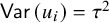 . Figure (b) shows a location-scale model on the heterogeneity variance with
$f_{yi} = \mu + u_i$
 and
$\mathsf {Var} \left ( u_i \right ) = \exp (\alpha _0 + \alpha _1 x_i)$
 . Panel (c) shows a location-scale model on both the mean and the heterogeneity variance with
$f_{yi} = \beta _0 + \beta _1 x_i + u_i$
 and
$\mathsf {Var} \left ( u_i \right ) = \exp (\alpha _0 + \alpha _1 x_i)$
 . The shaded areas represent the 95% predictive intervals of the true effect size.

Figure 6 Long description
A three-panel figure with a shared grid layout. Each panel has a horizontal x-axis labeled Predictor (x sub i) and a vertical y-axis labeled True effec size (f sub y i).
* Panel A shows a linear increase in the true effect size as the predictor increases. The shaded predictive interval maintains a constant width throughout the trend, representing a standard mixed-effects model.
* Panel B shows a horizontal flat line for the true effect size. The shaded predictive interval is wide on the left and narrows significantly as the predictor increases, representing a location-scale model on the heterogeneity variance.
* Panel C shows a linear increase in the true effect size similar to Panel A. However, the shaded predictive interval is wide at low predictor values and narrows as the predictor increases, representing a location-scale model applied to both the mean and the heterogeneity variance.
The location-scale models have been utilized in multilevel models.Reference Hedeker, Mermelstein and Demirtas
70
and SEMReference McNeish
71
Recently, Viechtbauer and López-LópezReference Viechtbauer and López-López
23
extended these models for meta-analysis. The core idea is to model the mean and variance structures separately. For example, Figure 6(b) depicts a model with an average effect where the heterogeneity decreases as
$x_i$
 increases. Conversely, Figure 6(c) illustrates that
$x_i$
 has a positive relationship with the expected mean but a negative relationship with the residual heterogeneity variances. These models are similar to the regression models with heteroskedasticity.
In the location-scale model with additive error, the model-implied variance and mean for the ith study are as follows:

where
$\tau ^2_0=\exp {(\alpha _0)}$
 is the residual heterogeneity variance when
$x_i=0$
 . An exponential function is typically employed to ensure that the predicted residual heterogeneity variance is nonnegative. The mean structure is identical to that in a standard meta-regression. The intriguing aspect is the variance structure. Although we use
$x_i$
 in this example’s mean and variance structures, the predictors can be different for these two structures.
The following R code implements the location-scale model in Equation (3.25). Lines 2–6 define a generic random-effects model with the average effect mu and residual heterogeneity variance tau2. Lines 8 and 9 define the linear relationship for mu and the nonlinear relationship for tau2. b0 (
$\beta _0$
 ) and b1 (
$\beta _1$
 ) are the regression coefficients in predicting the mean structure mu, whereas a0 (
$\alpha _0$
 ) and a1 (
$\alpha _1$
 ) are the regression coefficients in predicting the variance structure tau2. Since we aim to replace the parameters on the left-hand side with the expressions on the right-hand side, we need to add the replace.constraints = TRUE argument in the analysis (see the discussion in Section 3.1.4). After fitting the model, neither regression coefficient is statistically significant in predicting the mean and variance structures. The parameter estimates and their 95% Wald CIs are (
$\hat {\beta }_1=-0.0013, [-0.0031, 0.0005]$
 ) and (
$\hat {\alpha }_1=0.0054, [-0.0204, 0.0312]$
 ). The results are identical to those in the metafor package.
## Location-scale model with an additive heterogeneity variance
m12 <- "yi ~ mu*1                 ## Mean(yi) = mu
                      yi ~~ data.vi*yi   ## Var(ei) = vi
                      ## ui is the latent variable of the random effect
                      ui =~ 1*yi                ## yi = 1*ui
                      ui ~~ tau2*ui      ## Var(ui) = tau2 of the residual heterogenenity variance
                      ## Specify a linear relationship on the mean structure
                      mu == b0 + b1*data.xi
                      ## Specify a nonlinear relationship on the variance structure
                      tau2 == exp(a0 + a1*data.xi)
"
Since the location-scale model has been implemented in the metafor package, some readers may wonder about the necessity of implementing their own model given this existing functionality. The present SEM approach offers the flexibility to specify a wide range of arbitrary models tailored to specific research needs. For example, the location-scale model with two or more effect sizes can be easily accommodated within the SEM-based meta-analysis framework. Additionally, we can also explore models that have not yet been implemented in current software. For instance, to my knowledge, the location-scale model has not been extended to incorporate multiplicative error or hybrid models (cf. the studyReference Kulinskaya and Olkin 34 for other ideas). As an example, the following model-implied variance and mean in the ith study shows a location-scale model with a multiplicative error:

where
$\phi _0=\exp {(\alpha _0)}$
 is the heterogeneity scaling factor when
$x_i=0$
 . The implementation of the location-scale model with a multiplicative error is shown below. After fitting the model, the predictor is statistically significant in predicting the mean structure (
$\hat {\beta }_1=-0.0026$
 , 95% Wald CI =
$[-0.0047, -0.0005]$
 ) but not for the variance structure (
$\hat {\alpha }_1=-0.0110$
 , 95% Wald CI =
$[-0.0313, 0.0093]$
 ). In theory, we can also create a location-scale model for the hybrid model that incorporates both multiplicative and additive heterogeneity. Still, it is yet to be determined what the interpretations of the parameters are due to the large number of parameters involved.
## Location-scale model with a multiplicative heterogeneity variance
m13 <- "yi ~ mu*1                 ## Mean(yi) = mu
                      yi ~~ sigma2*yi    ## Var(yi) = sigma2
                      ## Specify nonlinear on mean and variance structures
                      mu == b0 + b1*data.xi
                      sigma2 == exp(a0 + a1*data.xi)*data.vi
"
4 Multivariate meta-analyses
In this section, we expand the univariate meta-analysis to a multivariate meta-analysis. Multivariate meta-analysis has been developed and applied for decades.Reference Berkey, Anderson and Hoaglin 72 – Reference Jackson, Riley and White 74 It is commonly used when a study contributes more than one conceptually distinct effect.Reference Cheung 75 For instance, there may be multiple treatment groups but only one control group in intervention or experimental studies. The effect sizes calculated from these multiple treatment groups are correlated because they all share the same control group.Reference Gleser, Olkin, Cooper, Hedges and Valentine 76 This sampling correlation needs to be considered when analyzing these effect sizes. In observational studies, correlation matrices are a natural form of multivariate meta-analysis.Reference Becker, Aloe, Cheung, Schmid, Stijnen and White 77 These matrices allow researchers to analyze the relationships between multiple variables simultaneously.
We use a sample dataset from Chan et al.Reference Chan, Jones, Hall Jamieson and Albarracín
78
to demonstrate models with a bivariate meta-analysis. These authors investigated the misinformation and the debunking effects. The primary studies included in the meta-analysis involved three groups of participants: (1) those exposed to a misinformation message, (2) those exposed to both the misinformation message and a debunking message, and (3) control participants who received neither message. To illustrate, we selected the standardized mean difference (Hedges’ g) for two effects: the misinformation effect (the standardized difference between groups 1 and 3) and the debunking effect (the standardized difference between groups 2 and 1). As group 1 was involved in calculating both effect sizes, their sampling errors were correlated.Reference Gleser, Olkin, Cooper, Hedges and Valentine
76
For convenience, we refer to the effects of misinformation and debunking as
$y_{1i}$
 and
$y_{2i}$
 , respectively. Additionally, we use the year of publication
$x_i$
 as a covariate in our illustrations.
The original study comprised 52 independent samples, each nested within one of eight research reports. We only selected two effect sizes for this illustration and excluded studies comparing groups 2 and 3. As a result, the final sample for our illustration comprises 34 independent samples, each nested within one of six research reports. It is worth noting that the data and analyses differ between Chan et al.’s original study and our current tutorial. Our focus is on demonstrating the techniques rather than providing substantive interpretations. Readers should refer to Chan et al.Reference Chan, Jones, Hall Jamieson and Albarracín 78 for more detailed analyses and interpretations.
4.1 Bivariate random-effects model by regressing a true effect on another true effect
Researchers sometimes aim to use one effect size to predict another effect size. In medical research, researchers investigate the effect of baseline risk (an effect size) on treatment benefit (another effect size).Reference Arends, Hoes, Lubsen, Grobbee and Stijnen 79 – Reference Guolo 83 Similar examples are also found in psychology. For instance,Reference Hart, Bailey, Luo, Sengupta and Watts 84 examined the follow-up effect size of intervention effects on social-emotional and cognitive skills in children and adolescents. These authors used the immediate treatment effect to predict the follow-up treatment effect. Another example is Chan and Albarracín,Reference Chan and Albarracín 85 a follow-up study of Chan et al.,Reference Chan, Jones, Hall Jamieson and Albarracín 78 which aimed to study the debunking effect while controlling for the misinformation effect. Researchers typically test these hypotheses using meta-regression, treating one effect size as a predictor while ignoring the known sampling variance of the predictor. As discussed in this article, this approach can lead to incorrect parameter estimates and SEs.
Figure 7 presents the structural equation model in Equation (4.1) that can correctly analyze such data. The central idea is to formulate the true effect sizes as two latent variables (
$f^{(1)}_i$
 and
$f^{(2)}_i$
 ). This allows for the straightforward inclusion of predictive relationships in the model:

The model-implied mean vector and covariance matrix in the ith study are

A structural equation model of a bivariate random-effects meta-analysis by regressing a true effect on another true effect.
Note:
$y^{(1)}_i$
 and
$y^{(2)}_i$
 are two effect sizes in the ith study. The terms
$u^{(1)}_i$
 and
$u^{(2)}_i$
 , as well as
$e^{(1)}_i$
 and
$e^{(2)}_i$
 , represent the two random effects and sampling errors in the ith study, respectively. The matrices
$\boldsymbol {T}$
 and
$\boldsymbol {V}_i$
 (specifically
$data.v11i$
 ,
$data.v21i$
 , and
$data.v22i$
 ) are the
$2\times 2$
 heterogeneity covariance matrix of the random effects and the known sampling error covariance matrix, respectively.
$\mu ^{(1)}$
 is the average effect of
$f^{(1)}_i$
 .
$\beta ^{(2)}_0$
 and
$\beta ^{(2)}_1$
 are the intercept and slope in regressing
$f^{(2)}_i$
 on
$f^{(1)}_i$
 .

Figure 7 Long description
The diagram is organized into three vertical columns.
* At the far left is a triangle containing the number 1. Two arrows originate from this triangle. The upper arrow is labeled mu super (1) and points to a circle. The lower arrow is labeled beta sub 0 super (2) and points to a second circle.
* In the center column are two circles representing latent variables. The top circle is labeled f sub i super (1) and has a self-loop arrow on top labeled T [1, 1]. The bottom circle is labeled f sub i super (2) and has a self-loop arrow at the bottom labeled T [2, 2]. A vertical arrow labeled beta sub 1 super (2) points from the top circle down to the bottom circle.
* In the right column are two shaded rectangles representing observed variables. The top rectangle is labeled y sub i super (1) and has a self-loop arrow labeled data dot V 11 i. The bottom rectangle is labeled y sub i super (2) and has a self-loop arrow labeled data dot V 22 i. A double-headed vertical arrow labeled data dot V 21 i connects these two rectangles.
* Horizontal arrows labeled with the number 1 connect the center circles to their corresponding right-side rectangles: f sub i super (1) points to y sub i super (1), and f sub i super (2) points to y sub i super (2).
The following R code implements this model. There are two important points worth discussing. First, we are estimating the means of the true effect sizes (
$f^{(1)}_i$
 and
$f^{(2)}_i$
 ) (lines 9 and 10) while the means of the observed effect sizes (
$y^{(1)}_i$
 and
$y^{(2)}_i$
 ) are fixed at 0 in line 3. Since we are regressing the true effect sizes, estimating the means of these true effect sizes is essential. Second, there is no T_21 in the (residual) heterogeneity covariance matrix (lines 19 and 20) because we have included the regression coefficient
$\beta ^{(2)}_1$
 in the model (line 22). After fitting the model, the estimated coefficients and their 95% Wald CIs are
$\hat {\beta }^{(2)}_0=-0.3621, [-1.0554, 0.3312]$
 and
$\hat {\beta }^{(2)}_1=0.6836, [0.4361, 0.9310]$
 . The estimated
$R^2$
 is
$0.7989, [0.5850, 1.0000]$
 , where the upper bound is truncated to 1.00.
## Prepare a dataset
dat2 <- data.frame(y1i=Chan17$g_misinfo,
                          y2i=Chan17$g_debunk,
                          V11i=Chan17$v_misinfo,
                          V21i=Chan17$c_mis_deb,
                          V22i=Chan17$v_debunk)

## Regressing true effect sizes f2i on f1i
m14 <- "## Means of y1 and y2 are fixed at 0
                      y1i + y2i ~ 0*1
                      ## Known sampling variances and covariance
                      y1i ~~ data.V11i*y1i
                      y2i ~~ data.V22i*y2i
                      y1i ~~ data.V21i*y2i
                      ## f1i and f2i: True effect sizes
                      f1i =~ 1*y1i
                      f2i =~ 1*y2i
                      ## Heterogeneity variances
                      f1i ~~ T_11*f1i
                      f2i ~~ T_22*f2i
                      ## Regressing f2i on f1i
                      f2i ~ b0*1+ b1*f1i
                      f1i ~ mu_1*1
                      ## Define R2 on f2i
                      R2 := b1^2*T_11/(b1^2*T_11 + T_22)
"
5 Discussion
This tutorial showed how various standard and advanced meta-analytic models can be expressed as structural equation models. The SEM-based meta-analysis offers a straightforward approach to defining models using equations, making it accessible to non-experts in meta-analysis. Once specified, these models can be converted into graphical models, which help understand the relationships between variables. Additionally, users can calculate the model-implied mean vector and covariance matrix, further enhancing their understanding of the fitted models. These components (equations, graphical models, and model-implied statistics) are valuable tools for users to comprehend the structure and assumptions of their meta-analytic models. Most importantly, users can fit the proposed models to their data using the FIML estimation method, which is efficient when missing data are MAR. This tutorial also highlighted the flexibility of SEM by showing that users can define new models among effect sizes that may not currently be available in standard meta-analysis packages. This ability allows researchers to explore innovative modeling approaches tailored to their research questions.
Despite the many appealing features of the SEM approach, it has some limitations that should be considered. Firstly, only the FIML estimation method is readily available, although it is possible to specify REML for some models. However, creating these models is not straightforward.Reference Cheung 29 Additionally, various estimators are used in meta-analysis (e.g., Hunter-Schmidt, Hedges, and DerSimonian-Laird),Reference Viechtbauer 27 and it is unlikely that they can be implemented within the SEM framework. Secondly, SEM uses a Wald or z-statistic to test parameter estimates, while most meta-analysis packages prefer a t-statistic, which generally performs better, especially in small sample sizes. Nevertheless, researchers can manually address this limitation by replacing the z-statistic with the t-statistic.Reference Lee and Beretvas 52
Another limitation concerns the handling of non-independent effect sizes. While extending the SEM-based meta-analysis to accommodate non-independent effect sizes is relatively straightforward using multivariate meta-analysis,Reference Cheung 9 other types of non-independence, such as nested effect sizes, pose additional challenges. A SEM-based three-level meta-analysis has been proposed and implemented in the metaSEM package,Reference Cheung 10 but it is currently limited to only one effect size. Specifying three-level meta-analyses with multiple effect sizes using equations has yet to be implemented. Users who wish to conduct such analyses can still implement them using the OpenMx code.Reference Pritikin, Hunter, Tv, Brick and Boker 86 Additionally, the popular robust variance estimation (RVE) methodReference Hedges, Tipton and Johnson 87 , Reference Pustejovsky and Tipton 88 in meta-analysis has not been implemented for SEM-based meta-analysis. Future research should explore these directions to expand the capabilities and applicability of SEM in meta-analysis.
In conclusion, this tutorial demonstrates that SEM-based meta-analysis is a flexible and powerful tool for learning about and conducting meta-analyses. It can supplement existing meta-analysis tools to address complex research questions. Despite its limitations, SEM offers unique advantages in specifying, visualizing, and fitting sophisticated meta-analytic models. The SEM-based meta-analysis holds great promise as a favorable framework for conducting future meta-analyses.
Acknowledgements
Part of this research was presented at the Annual Meeting of the Society of Research Synthesis Methodology in June 2024 in Amsterdam, the Netherlands, and at the Australasian Mathematical Psychology Conference in February 2026 in Singapore.
Author contributions
Conceptualization: M.W.-L.C.; Data curation: M.W.-L.C.; Data visualization: M.W.-L.C.; Methodology: M.W.-L.C.; Writing—original draft: M.W.-L.C.
Competing interests
The author declares that no competing interests exist.
Data availability statement
Complete examples and R code are available on Zenodo at https://doi.org/10.5281/zenodo.20962641.
Funding statement
This research was supported by a grant from the Singapore Ministry of Education Academic Research Fund Tier 1 (FY2021-FRC1-008).
Ethical standards
The research meets all ethical guidelines, including adherence to the legal requirements of the study country.
Disclosure of use of AI tools
ChatGPT and Grammarly were used to check grammar and improve the writing.
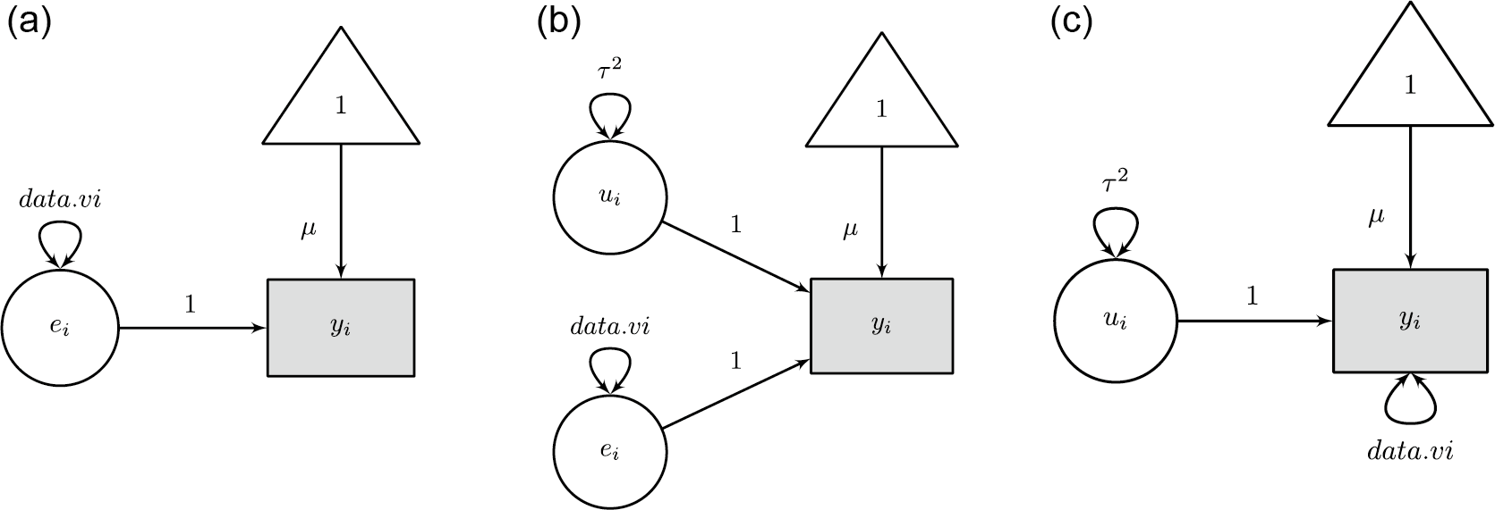


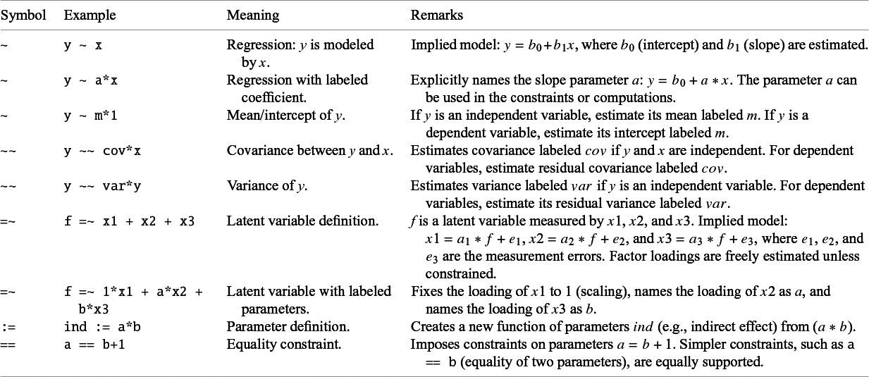
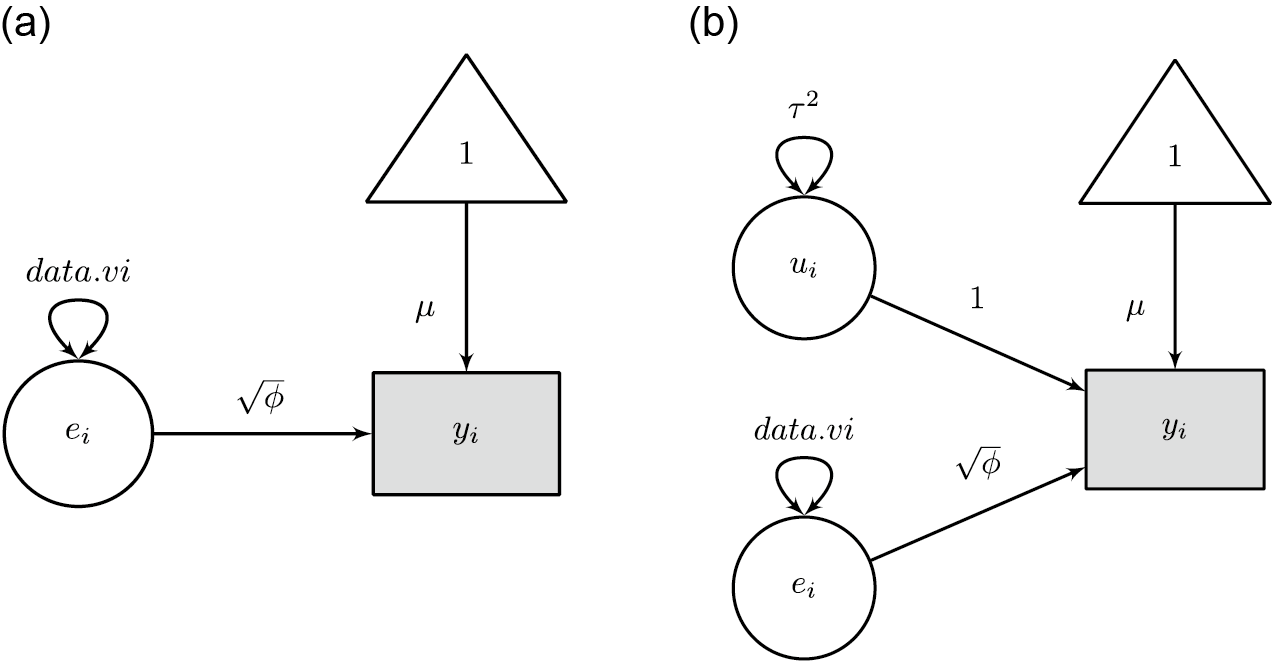


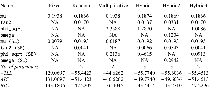
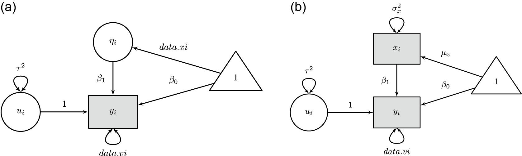


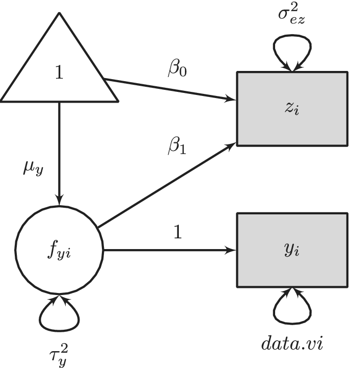


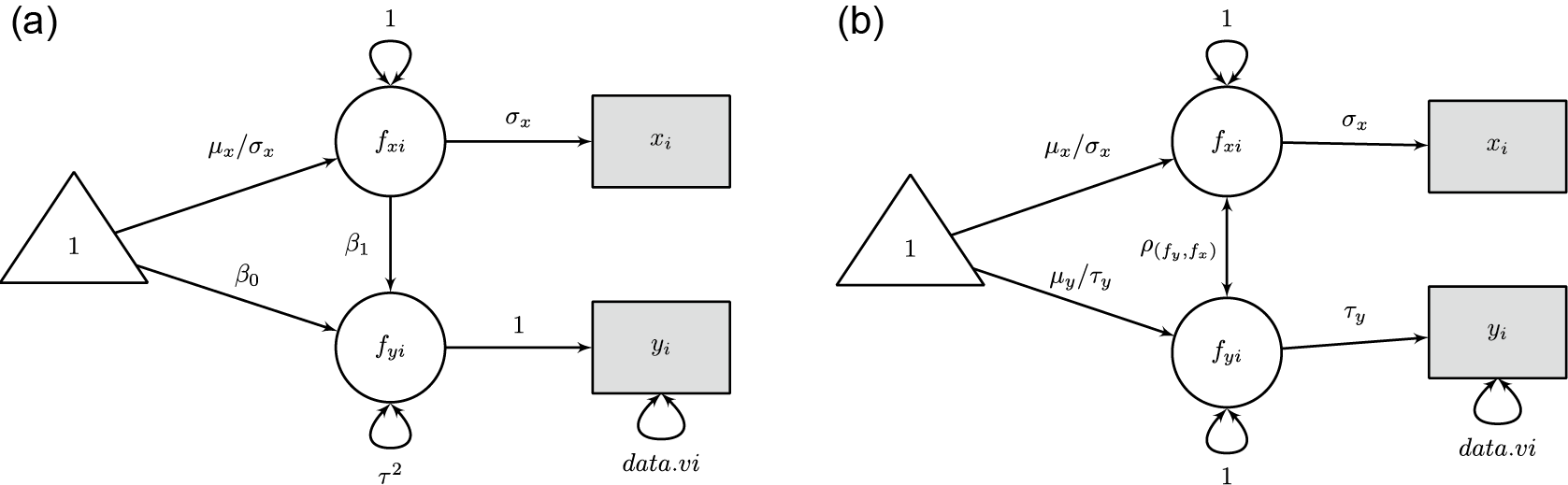


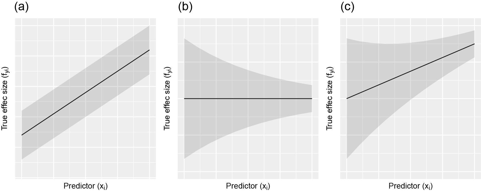


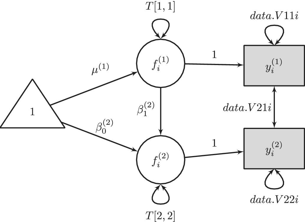


 Open access

